MINIMIZING THE UNCERTAINTIES IN DEPTH PREDICTION

OFCARBONATESTRUCTUREIN

CENTRAL LUCONIA PROVINCE, OFFSHORE SARA W AK

MAZLAN BIN MD TAHIR

PETROLEUM GEOSCIENCE

UNIVERSITI TEKNOLOGI PETRONAS

JANUARY 2008

STATUS OF THESIS

MINIMIZING THE UNCERTAINTIES IN DEPTH PREDICTION

OFCARBONATESTRUCTUREIN

CENTRAL LUCONIA PROVINCE, OFFSHORE SARA W AK

I, MAZLAN BIN MD TAHIR hereby allow my thesis to be placed at the

Information Resource Center (IRC) of Universiti Teknologi PETRONAS (UTP) with

the following conditions:

I. The thesis becomes the property ofUTP

2. The IRC ofUTP may make copies of the thesis for academic purposes only

3. The thesis is classified as

~ Confidential

D Non-confidential

If this thesis is confidential, please state the reason:

As instructed by Petroleum Management Unit (PMU), PETRONAS

The contents of the thesis will remain confidential for __________ years.

Remarks on disclosure:

Endorse by

Petroleum Resource Assessment and Marketing, Petroleum Management Unit, Petroliam Nasional Berhad, Level 22, Tower 2, PETRONAS Twin Towers, Kuala Lumpur City Centre, 50088 Kuala Lumpur

Date: 18th February 2008

Petroleum Resource Assessment and Marketing, Petroleum Management Unit, Petroliam Nasional Berhad, Level 22, Tower 2, PETRONAS Twin Towers, Kuala Lumpur City Centre, 50088 Kuala Lumpur

Date: 18th February 2008

APPROVAL PAGE

UNIVERSITI TEKNOLOGI PETRONAS

Approval by Supervisor (s)

The undersigned certify that they have read, and recommend to The Postgraduate

Studies Programme for acceptance, a thesis entitled "Minimizing the

Uncertainties in Depth Prediction of Carbonate Structure in Central

Luconia Province, Offshore Sarawak" submitted by Mazlan bin Md Tahir for

the fulfilment of the requirements for the degree of master of science in

Petroleum Geoscience.

\ '

Date: 18th February 2008

Signature

Main Supervisor En. Che Shaari Abdullah

Date 18th February 2008

Co-Supervisor 1

Co-Supervisor 2

11

J

TITLE PAGE

UNIVERSITI TEKNOLOGI PETRONAS

MINIMIZING THE UNCERTAINTIES IN DEPTH PREDICTION

OF CARBONATE STRUCTURE IN

CENTRAL LUCONIA PROVINCE, OFFSHORE SARA W AK

By

MAZLAN BIN MD TAillR

A THESIS

SUBMITTED TO THE POSTGRADUATE STUDIES PROGRAMME

AS A REQUIREMENT FOR THE

DEGREE OF MASTER OF SCIENCE

IN PETROLEUM GEOSCIENCE

BANDAR SERI ISKANDAR,

PERAK

JANUARY, 2008

111

DECLARATION

I hereby declare that the thesis is based on my original work except for quotations and

citations which have been duly acknowledged. I also declare that it has not been

previously or concurrently submitted for any other degree at UTP or other institutions.

Signature

Name

Date

Mazlan bin Md Tahir

181h February 2008

IV

ACKNOWLEDGEMENT

I am very grateful to my supervisor, En. Che Shaari Abdullah (Staff Geoscientist,

PRAM, PMU, PETRONAS) for his interesting insight and invaluable guidance. Also,

I would like to thank Mr. Mike Brumby (Director and Asian Regional Manager,

Petrosys), Mr. Ji Ping (Manager, PRAM, PMU, PETRONAS) and Mr. Alwyn Chung

Kwang Tjet (Geoscientist, PRAM, PMU, PETRONAS) for their constructive

criticism and fruitful discussion as well as to my colleagues for their support.

v

ABSTRACT

The objective of this case study is to reduce the uncertainties in depth prediction of

the target carbonate reservoir by mapping optimum interval velocities in the overlying

sequences. Lithology facies variations have very significant impact on the lateral and

vertical velocity behaviour of geologic formation. The area covering Block SK316

and SK31 0, offshore Sarawak, East Malaysia where the carbonate pinnacle structure

is the target reservoir has been chosen for the study. Five major horizons had been

identified and interpreted which are Seabed, Near Cycle VII, Near Cycle VI, Near

Cycle V and Near Cycle IV (Top of carbonate) using the seismic line vintage 1994.

Two softwares had been used in this case study which are SeisWorks, Landmark

Graphic software (for interpretation purposes) and Petrosys software (for mapping

purposes). By finding the interval velocity models for the major stratigraphic

sequences and depth structure map of the target reservoir, we can improve the depth

structure map of the carbonate pinnacle reservoir and reduce the uncertainties in

hydrocarbon volume estimation.

VI

ABSTRAK

Objektif kajian kes ini adalah untuk mengurangkan ketidakpastian didalam

meramalkan kedalaman sasaran takungan karbonat. Ini dapat dilakukan dengan proses

pemetaan halaju selang yang optimum bagi setiap lapisan. Variasi terhadap fasies

litologi memberi kesan yang penting bagi sifat atau tingkah laku halaju secara

menegak dan sisian didalam pembentukan geologi. Kawasan Blok SK316 dan SK31 0

di luar persisiran Sarawak telah dipilih dalam kajian kes ini di mana sasaran takungan

adalah merupakan karbonat yang mempunyai struktur berbentuk puncak. Lima

lapisan tanah telah dikenalpasti dan ditafsirkan adalah "Seabed", "Near Cycle VII",

"Near Cycle VI", "Near Cycle V" dan "Near Cycle IV" (Kemuncak karbonat)

dengan menggunakan garisan seismos 1994. Dua perisian komputer telah digunakan

didalam kajian kes ini iaitu perisian SeisWorks, Landmark Graphic (digunakan untuk

tujuan pentafsiran) dan perisian Petrosys (digunakan untuk tujuan pemetaan). Dengan

mencari model halaju selang bagi setiap susunan stratigrafik utama dan peta struktur

kedalaman sasaran takuangan, kita dapat memperbaiki peta struktur kedalaman bagi

takungan karbonat berbentuk puncak dan juga dapat mengurangkan ketidakpastian

didalam membuat anggaran isipadu hidrokarbon.

vii

...J

STATUS OF THESIS APPROVAL PAGE TITLE PAGE DECLARATION ACKNOWLEDGEMENT ABSTRACT ABSTRAK TABLE OF CONTENTS LIST OF TABLES LIST OF FIGURES LIST OF SYMBOLS LIST OF ABBREVIATIONS

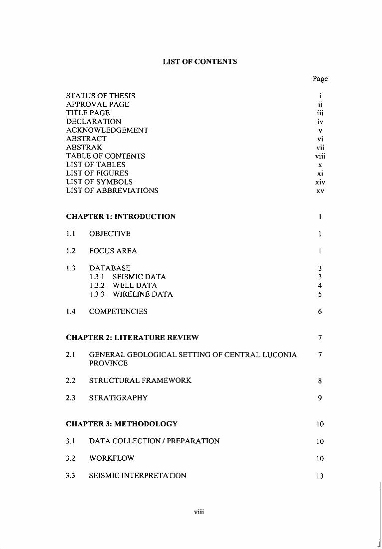
LIST OF CONTENTS

CHAPTER 1: INTRODUCTION

1.1 OBJECTIVE

1.2 FOCUS AREA

1.3 DATABASE 1.3.1 SEISMIC DATA 1.3.2 WELL DATA 1.3.3 WIRELINE OAT A

1.4 COMPETENCIES

CHAPTER 2: LITERATURE REVIEW

Page

II

Ill

IV

v VI

VII

VIII

X

XI

XIV

XV

3 3 4 5

6

7

2.1 GENERAL GEOLOGICAL SETTING OF CENTRAL LUCONIA 7 PROVINCE

2.2 STRUCTURAL FRAMEWORK 8

2.3 STRATIGRAPHY 9

CHAPTER3:METHODOLOGY 10

3.1 DATA COLLECTION I PREPARATION 10

3.2 WORKFLOW 10

3.3 SEISMIC INTERPRETATION 13

VIII

3.4 TIME-DEPTH RELATIONSHIP MODELING 14

3.5 INTERVAL VELOCITY CALCULATION 17

3.6 MAPPING 18

CHAPTER 4: RESULT & DISCUSSION 19

4.1 STUDY AREA EXTENT 19

4.2 TWT CONTOUR MAP 22

4.3 ISOCHRON CONTOUR MAP 25

4.4 INTERVAL VELOCITY CONTOUR MAP 27

4.5 ISOPACH CONTOUR MAP 30

4.6 DEPTH CONTOUR MAP (NOT TIED TO WELL) 33

4.7 DEPTH CONTOUR MAP (TIED TO WELL) 37

4.8 DEPTH CORRECTIONS 40

4.9 RESULTS 43 4.9.1 INTERVAL VELOCITY MODELS 43 4.9.2 DEPTH STRUCTURE MAP OF THE TARGET 44

RESERVOIR

4.10 COMPARISON IN DEPTH CONTOUR MAP USING 45 DIFFERENT TYPE OF VELOCITY

4.11 BLIND WELL TEST 48

CHAPTER 5: CONCLUSION & RECOMMENDATION 49

5.1 CONCLUSION 49

5.2 RECOMMENDATION 50

REFERENCES 51

APPENDIX 1 52

APPENDIX2 62

APPENDIX3 66

IX

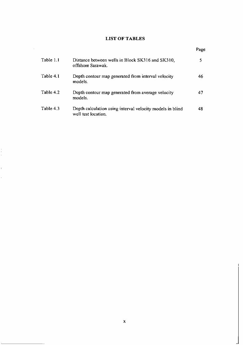
Table 1.1

Table 4.1

Table 4.2

Table 4.3

LIST OF TABLES

Distance between wells in Block SK316 and SK31 0, offshore Sarawak.

Depth contour map generated from interval velocity models.

Depth contour map generated from average velocity models.

Depth calculation using interval velocity models in blind well test location.

X

Page

5

46

47

48

LIST OF FIGURES

Page

Fig. 1.1 Location of case study in East Central Luconia Province 2 (yellow), offshore Sarawak in Block Sk316 and SK 310. Small map at the upper right corner is a map of Malaysia.

Fig. 1.2 Zoom-in area of case study location in Block SK316 and 2 SK31 0, offshore Sarawak.

Fig. 1.3 Seismic line vintage 88, 93 and 94 in Block SK316 and 3 SK31 0, offshore Sarawak.

Fig. 1.4 Location of the wells in Block SK316 and SK31 0, offshore 4 Sarawak.

Fig. 1.5 Example of wire line data ( GR (green) and Sonic (white or 5 blue)) in well NCI0-1 and PC4-1 that have been used to identifies and to help in each horizon interpretation.

Fig. 2.1 Location of Central Luconia province relative to other 8 major province of Northern Borneo (M. Yamin, 1999; Abolins P., 1999).

Fig. 2.2 Stratigraphic section at Seismic data vintage 94, line 9 94CL-1075.

Fig. 3.1 General workflow of case study. II

Fig. 3.2 Workflow to generate the interval velocity map on each 12 layer.

Fig. 3.3 Workflow to generate depth contour map of each horizon. 12

Fig. 3.4 Interpreted horizons at Seismic line 94CL-1075. 14

Fig. 3.5 Time-Depth Table Display for well NC10-l in SeisWorks 15 software.

Fig. 3.6 Time-Depth Table Display for well PC4-1 in SeisWorks 16 software.

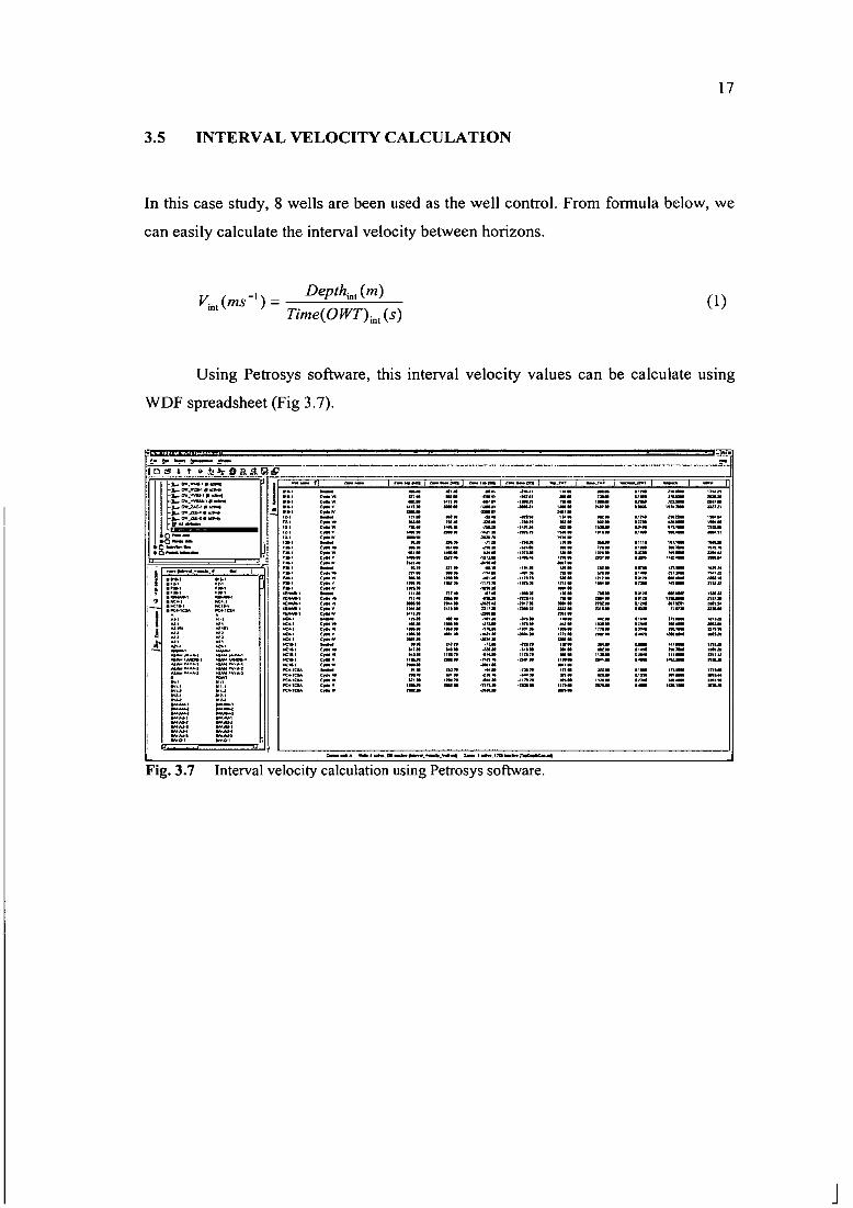
Fig. 3.7 Interval velocity calculation using Petrosys software. 17

Fig. 4.1 Area interpreted for Seabed ( 100- 500 msec ). 19

Fig. 4.2 Area interpreted for Near Cycle VII (200- 2000 msec). 20

Fig. 4.3 Area interpreted for Near Cycle VI (400- 3000 msec). 20

XI

J

Fig. 4.4 Area interpreted for Near Cycle V (400- 3000 msec). 21

Fig. 4.5 Area interpreted for Near Cycle IV ( 1500 - 3900 msec ). 21

Fig. 4.6 Seabed TWT contour map. 22

Fig. 4.7 Near Cycle VII TWT contour map. 23

Fig. 4.8 Near Cycle VI TWT contour map. 23

Fig. 4.9 Near Cycle V TWT contour map. 24

Fig.4.10 Near Cycle IV TWT contour map. 24

Fig. 4.11 Seabed and Near Cycle VII isochron contour map. 25

Fig.4.12 Near Cycle VII and Near Cycle VI isochron contour map. 26

Fig. 4.13 Near Cycle VI and Near Cycle V isochron contour map. 26

Fig.4.14 Near Cycle V and Near Cycle IV isochron contour map. 27

Fig. 4.15 Interval velocity between Seabed and Near Cycle VII 28 contour map.

Fig.4.16 Interval velocity between Near Cycle VII and Near Cycle 28 VI contour map.

Fig. 4.17 Interval velocity between Near Cycle VI and Near Cycle V 29 contour map.

Fig.4.18 Interval velocity between Near Cycle V and Near Cycle IV 29 contour map.

Fig. 4.19 An example of Grid Formula that been used to generate 30 Seabed and Near Cycle VII isopach contour map in Petrosys software.

Fig. 4.20 Seabed and Near Cycle VII isopach contour map. 31

Fig. 4.21 Near Cycle VII and Near Cycle VI isopach contour map. 31

Fig. 4.22 Near Cycle VI and Near Cycle V isopach contour map. 32

Fig. 4.23 Near Cycle V and Near Cycle IV isopach contour map. 32

Fig. 4.24 An example of Grid Formula that been used to generate 33 Seabed depth contour map in Petrosys software.

Fig. 4.25 Seabed depth contour map. 34

Xll

L

Fig. 4.26 Near Cycle VII depth (not tied) contour map. 35

Fig. 4.27 Near Cycle VI depth (not tied) contour map. 35

Fig. 4.28 Near Cycle V depth (not tied) contour map. 36

Fig. 4.29 Near Cycle IV depth (not tied) contour map. 36

Fig. 4.30 An example of WDF spreadsheet in Petrosys that shows 37 actual depth data on each horizon in all wells in the Block SK316 and SK310.

Fig. 4.31 Seabed depth (tied to all wells) contour map. 38

Fig. 4.32 Near Cycle VII depth (tied to all wells) contour map. 38

Fig. 4.33 Near Cycle VI depth (tied to all wells) contour map. 39

Fig. 4.34 Near Cycle V depth (tied to all wells) contour map. 39

Fig. 4.35 Near Cycle IV depth (tied to all wells) contour map. 40

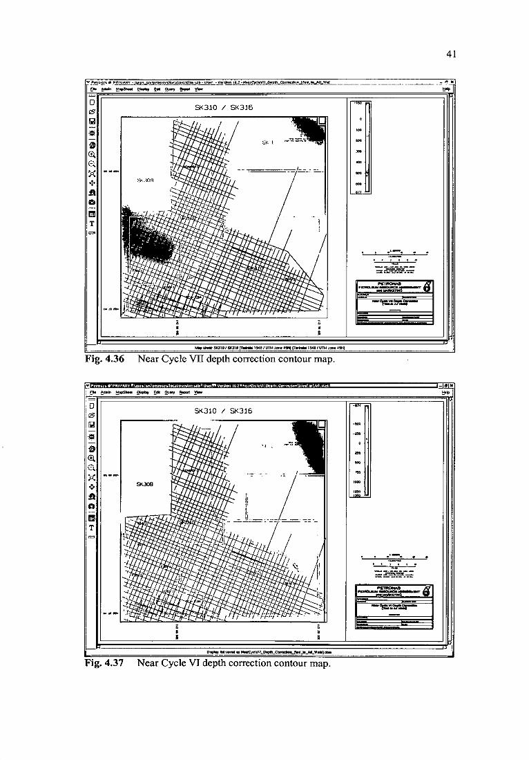
Fig. 4.36 Near Cycle VII depth correction contour map. 41

Fig. 4.37 Near Cycle VI depth correction contour map. 41

Fig. 4.38 Near Cycle V depth correction contour map. 42

Fig. 4.39 Near Cycle IV depth correction contour map. 42

Fig. 4.40 Interval velocity contour map of each layer; Seabed & 43 Near Cycle VII, Near Cycle VII & Near Cycle VI, Near Cycle VI & Near Cycle V and Near Cycle V and Near Cycle IV.

Fig. 4.41 Near Cycle IV (Top of carbonate) depth contour map (tied 44 to all wells).

Fig. 4.42 Workflow for depth map generated from different type of 45 velocity.

X111

J

LIST OF SYMBOLS

km kilometer

m meter

Ma million years

msec orms millisecond

sec or s second

v velocity

& and

0 degree

minutes

II second

XIV

LIST OF ABBREVIATIONS

2D Two dimension

GR Gamma Ray

Int Interval

INTVEL Interval velocity

KB Kelly Bushing

Max Maximum

MD Measured depth

Min Minimum

MSL Mean Sea Level

NE North West

NNE North North East

OKING OK/NotGood

OWT One way time

ss Subsea

ssw South South West

TD Total depth

TVD True vertical depth

TWT Two-way-time

T-Z Time-Depth

UTM Universal Transverse Mercator

VSP Vertical Seismic profile

WDF Petrosys Well Data Editor File

XV

CHAPTER!

INTRODUCTION

1.1 OBJECTIVE

The objective of this case study is to reduce the uncertainties in depth prediction by

finding optimum velocity on each layer. This is because of variations of vertical and

lateral velocity. The vertical and lateral velocity variations introduce significant

uncertainties in reservoir depth prediction and depth structure mapping of carbonate

pinnacle in Central Luconia province, offshore Sarawak. By finding optimum velocity

model, it can refine the accuracy.

1.2 FOCUS AREA

The area of this case study is in East Central Luconia province, offshore Sarawak in

Block SK316 and SK31 0 (Fig. 1.1 and Fig. 1.2). The area size is approximately 2820

krn2 with water depths ranging from 70 m to 118 m and the main reservoirs here are

carbonates of Miocene age.

2

-tJ• Help

Fig. 1.1 Location of case study in East Central Luconia province (yellow), offshore Sarawak in Block SK316 and SK310. Small map at the upper right comer is a map of Malaysia.

Fig. 1.2 Zoom-in area of case study location in Block SK316 and SK310, offshore Sarawak.

3

1.3 DATABASE

1.3.1 SEISMIC DATA

Seismic data (2D) vintage 88, 94 and 93 have been used is this case study (Fig. 1.3).

But, interpreted horizons tracking is based only on seismic line vintage 94. Seismic

line vintage 88 and vintage 93 have seismic misties problems due to difference in

acquisition and processing parameters.

The seismic line vintage 94, data quality is considered good from seabed down

to top of carbonate (Near Cycle IV) and seismic markers are relatively easy to

correlate. But in NE of Block SK316, the seismic data is poor because of major fault

zone. Below the carbonate layer (Near Cycle IV), the seismic quality deteriorates (Fig

1.6).

Fig. 1.3 Seismic line vintage 88, 93 and 94 in Block SK316 and SK31 0, offshore Sarawak.

4

1.3.2 WELL DATA

Eight wells, Kenari-1, NC4-1 , F2-1 , F39-l, F38-l, NCl0-1, PC4-l and B16-1 have

been chosen as well control for this case study. Below are locations of those wells

(Fig. 1.4)

~. - . - I

D ~

51<310 / SK315

r.;!)

c f» <tl. t:.."l .... "d' ~ .

•:0 9<308

.f1 D

1!11 T

"""

.. ~--. ' . . . .

Fig. 1.4 Location ofthe wells in Block SK316 and KS310, offshore Sarawak.

The distance between these wells in Block SK316 and SK31 0 has been

identified (Table 1.1 ). From the table, the nearest well is about 8 km between NC4-1

and F2-1 and the furthest is about 62 km between F2-1 and B 16-1.

5

F39-1 F38-1 F2-1 NC4-1 KENARI-1 816-1

24235 17842 30610 37290 52532 38527

NC10-1 9906 21341 28934 49040 47896

F39-1 24235 12347 20736 46570 59780

F38-1 17842 9906 19525 39545 49058

F2-1 30610 21341 12347 35078 60092

NC4-1 37290 28934 20736 19525 62570

KENARI-1 52532 49040 46570 39545 35078

816-1 38527 47896 59780 49058 60092 62570

Table 1.1 Distance between wells in Block SK316 and SK31 0, offshore Sarawak.

1.3.3 WIRELINEDATA

Wireline data such as GR and Sonic data of each well are also used for interpretation

purposes.

Fig. 1.5 An example of wireline data (GR (green) and Sonic (white or blue)) in NC 10-1 and PC4-l well that have been used to identify and to help in each horizon interpretation.

6

1.4 COMPETENCIES

The competencies required are as follows:

1. Proficiency in velocity concept and wire line sonic data analysis.

11. Familiarity in using workstation based seismic interpretation- SeisWorks,

Landmark Graphic software.

111. Skill in using mapping software- Petrosys software.

L

CHAPTER2

LITERATURE REVIEW

2.1 GENERAL GEOLOGICAL SETTING OF CENTRAL LUCONIA

PROVINCE

7

Central Luconia provmce m offshore Sarawak lies immediately North of

Balingian Province and is flanked by the clastic depocenters of the Baram Delta to the

East and the West Luconia Province to the west (Fig. 2.1). Relatively stable

conditions have prevailed since early Middle Miocene time.

The area is characterised by fairly continuous subsidence and is unaffected by

strong folding. The most important features of the Province are the Middle Miocene

carbonate reef buildups. The tops of the main carbonates form a diachronous horizon,

younger in the North and older to the South. The reefs are flanked and overlain by

clastic sequences of the same or younger age, resulting from an overall northwards

regional regression during the Middle Miocene (Ho, 1978; Doust, 1981 ).

The Central Luconia province is a broad and stable continental shelf platform,

characterised by extensive development of Late Miocene carbonates. More than 2000

carbonate buildups have been seismically mapped and some 65 buildups have been

tested (M. Yam in, 1999; Abolins P ., 1999)

110°(

F

WEST LUCONIA DELTA

SK.301

WEST WCONIA

RIM

.. -

8

112"( 114°(

- .J:_ SK307 I

~_j

Fig. 2.1 Location of Central Luconia province relative to other major province of Northern Borneo {M. Yamin 1999; Abolins P., 1999).

2.2 STRUCTURAL FRAMEWORK

The province is characterised by a network of NNE - SSW trending faults which

divide the zone into a somewhat elevated central block with flanking depressions and

basinal areas. To the East and West, the basin floor descends below younger deltaic

sediments associated with the Baram Delta and the East Natuna area.

The principal localised structures are associated with the pinnacles and the

flat-topped mounds and platform.

9

2.3 STRATIGRAPHY

Carbonate deposition began during the widespread subsidence of the Middle Miocene

(Cycle IV) at a time when this part of the shelf lay well away from the coastline and

in an open marine environment. Bank deposits to thickness of 200-300 meters were

developed on areas of structural elevation. Maximum transgression took place during

the Middle to Upper Miocene (Cycle V) and widespread reefs and reef-associated

carbonates were developed (Epting, 1980).

Some carbonate buildups exceed 20 kilometers in length and 1.5 kilometers in

thickness. During this period, the Baram and Rajang-Lupar deltas began to prograde

offshore and by the end of Near Cycle V had extended over much of Balingian and

the Southern part ofLuconia, burying several of the smaller buildups in their path (M.

Yamin, 1999; Abolins P., 1999). Below is the stratigraphic section of this case study

(Fig. 2.2).

Fig. 2.2 Stratigraphic section at Seismic data vintage 94, line 94CL-1075.

10

CHAPTER3

METHODOLOGY

3.1 DATA COLLECTION I PREPARATION

Data gathering started from the first week of August. The data included the reports

from PETRONAS UDRS, well data, paper review, etc. All seismic lines were already

loaded in the workstation as this is a continuation of the project that was done in 2005

by Petroleum Management Unit (PMU), PETRONAS.

3.2 WORKFLOW

Below is the general workflow of this case study (Fig. 3 .I). Inputs such as seismic

data (vintage 88,93 and 94), wells data (Kenari-1, NC4-1, F2-l, F39-l, F38-l, NCI0-

1, PC4-l and B16-1) and wireline data (GRand Sonic) were loaded into the server

workstation. Well to seismic tie was done on each well. This is to tie on seismic lines

(time domain) and the top of geological formations identified on the wireline well

logging interpretation (depth domain) by using time-depth relationship.

By knowing the time-depth relationship from the VSP or checkshot of each

well, we can estimate the depth of each horizon interpreted. From here, we can do the

gridding and contouring process to generate the interval velocity map and depth

structure map.

Workflow I shows precise detail to generate the interval velocity map (Fig.

3.2). Workflow 2 shows the detail to generate depth map of each horizon (Fig. 3.3).

General Workflow:

en !!!.

~ 0 ., ;II" Ill Ill

f Cil

"'0 CD -0 Ill '< Ill Ill

~ ~ ., CD

Interpretation

Export to

Mapping

11

r·-·-·--------.-_._-....... -... - .. -_._ .......... -.-.-.. -~-·---·-·-·----·---·-·; ! Seismic line/section, wells, wireline data j i_._._._._._. ___ ._._,_._._._._._,_,_._._._._.._,_,_,_._,_._._._._._._._._._.l

r·--·-·-·~--·-----------·-------·-·--------.......... -.. -·-·--·---·-·1 : l ( Individual interpretation ! ( ~ 1·-·-·-·-·-·--·---·--·----·--·-·-·-·-·-·-·--·-·-·-------·-·-·-·i

~-----·-·-·-·-·--·---·-·--·-·-·----·-·----·---------·-·--·-·~

i VSP or checkshot of each well I I -~ -----·-·-----·---·--·-·----·--·------------._:.1

r-·-·---... -.---_._-..-.-... -_._-.._-.-.._-.-·---·---·-·-·-·-.. --.---·-.. -~.-.-.., i l 1 Gridding and contouring process j ~--·-·------·-·-·-----·-·-- _______ ,

QC

,-. --·-- ----·-·-· ---·- ---1 I 11'. Change parameter: grid cell size;

1 compute, tie and correction process L_, ________________________ _l

r--·--·-·---·-----------------·--·----------, j Interval velocity map, Depth structure ~~ I map L-------------·--------·----

Fig. 3.1 General workflow of case study.

Workflow 1:

Compute Interval Velocity

Fig. 3.2 Workflow to generate the interval velocity map on each layer.

Workflow 2:

I Interval Velocity I I lsochron•

I Maps I I Maps

Isopach' Maps

Depth Maps of each Horizon

(not tie)

I Addition

I ·Tie process

• Correction process

Depth Maps of each Horizon

(tied to 8 wells)

Fig. 3.3 Workflow to generate depth contour map of each horizon.

12

13

3.3 SEISMIC INTERPRETATION

The seismic interpretation was done using SeisWorks, Landmark Graphic software. It

took about 2 months to interpret all horizons (Seabed, Near Cycle VII, Near Cycle VI,

Near Cycle V, Near Cycle IV). The interpreted horizons are based on the

unconformity picking on the seismic section (Homewood, 1999), GR and Sonic curve

of each well (Schlumberger, 1989). In this case study, five (5) horizons as follows had

been identified and interpreted (Fig. 3.4):

1. Seabed

11. Near Cycle VII

iii. Near Cycle VI

tv. Near Cycle V

v. Near Cycle IV (Top of carbonate)

Each horizon tracking is based on seismic line vintage 94 only. Seismic line

vintage 93 and vintage 88 have seismic misties problems due to difference in

acquisition and processing. Interpretation was not attempted in NE of block SK316

due to poor seismic data, results of major fault zone.

Well NCl0-1 and PC4-l are used as main well control (Fig. 3.4).

J

14

., _, . [fte '!!lew ~efsmle !!orlzons F!Ufts ~ens Help

)JHE: SPII: TIIACE: Z: A: X: V:

Fig. 3.4 Interpreted horizons at Seismic line 94CL-1 07 5.

3.4 TIME-DEPTH RELATIONSHIP MODELING

Interpretation was done on seismic section in time domain. But, in real life, wells are

drilled in depth domain. Here, we need to know the time-depth relationship. Thus, we

can estimate and know the prediction depth of the horizon interpreted. Below are 2

examples of Vertical Seismic Profile (VSP) and checkshot taken at well NC 10-1 and

well PC4-1 (Fig. 3.5 and Fig. 3.6).

15

WeD: NCI0-1 , NCI0-1

KeDy bushing (KB) elevauon: 27.00 m. Project datum elevauon: O.Om.

T-D table: PC4CSAedit T-D table datum elevation: O.Om. WeiUcurve shift: 0.0 msec

Decimated? NO

Depth/elevation units: v Feet • Meters Velocity units: v FeeUSec • Meters/Sec

Change Datum ... I Save As ... I

T-D datum T-D datum KB Relative Subsea Display Interval 2-Yiay Tune TVD (msec) TVD TVD TIME Velocity

o.o o.ooo 27.0 o.o o.ooo ~ 79.0 108.000 106.0 -79.0 108.000 1463.0

253.0 310.700 280.0 -253.0 310.700 1716.8 313.0 374.000 340.0 -313.0 374.000 1895.7 373.0 436.800 400.0 -373.0 436.800 1910.8 433.0 497.400 460.0 -433.0 497.400 1980.2 493.0 555.900 520.0 -493.0 555.900 2051.3 553.0 610.200 580.0 -553.0 610.200 2209.9 613.0 668.500 640.0 -613.0 668.500 2058.3 673.0 722.700 700.0 -673.0 722.700 2214.0 733.0 772.900 760.0 -733.0 772.900 2390.4 793.0 823.100 820.0 -793.0 823.100 2390.4 853.0 869.200 880.0 -853.0 869.200 2603.0 913.0 919.300 940.0 -913.0 919.300 2395.2 973.0 967.400 1000.0 -973.0 967.400 2494.8

1033.0 1019.500 1060.0 -1033.0 1019.500 2303.3 1093.0 1071.600 1120.0 -1093.0 1071.600 2303.3 1153.0 1127.600 1180.0 -1153.0 1127.600 2142.9 1213.0 1181.700 1240.0 -1213.0 1181.700 2218.1 1273.0 1223.700 1300.0 -1273.0 1223.700 2857.1 1333.0 1265.800 1360.0 -1333.0 1265.800 2850.3 1393.0 1307.800 1420.0 -1393.0 1307 .BOO 2857.1 1453.0 1347.900 1480.0 -1453.0 1347.900 2992.5 1513.0 1385.900 1540.0 -1513.0 1385.900 3157.9 1573.0 1428.000 1600.0 -1573.0 1428.000 2850.4 1633.0 1466.000 1660.0 -1633.0 1466.000 3157.9 1693.0 1504.000 1720.0 -1693.0 1504.000 3157.9 1753.0 1540.100 1780.0 -1753.0 1540.100 3324.1 1813.0 1576.100 1840.0 -1813.0 1576.100 3333.3 1873.0 1610.100 1900.0 -1873.0 1610.100 3529.4 ·" u.o II( 1~7.0 u.o l~ooo

Calculate Values I OIJ'rent values extrapolated? N 0

Fig. 3.5 Time-Depth Table Display for well NCIO-lin SeisWorks Software.

.J

16

Well: PC4-1 CSA , PC4-1 CSA

Kelly bushing (KB) elevation: 27.00 m. PI'Uject datum elevation: 0.0 m.

T-D table: csaPC4Edited T-D table datwn elevation: 0.0 m. WeD/curve shift: 0.0 msec

Decimated? NO

Depth/elevation units: v Feet ~ Meters Velocity units: v Feet/Sec ~ Meters/Sec

Change Datum .. ~ I Save As ... I

T-D datum T-D datum KB Relative Subsea Display Interval 2-Yiay Time TVD (msec) TVD TVD TIME Velocity

o.o o.ooo 27.0 o.o o.ooo ] 79.0 97.000 106.0 -79.0 97.000 1628.9

253.0 310.700 280.0 -253.0 310.700 1628.5 313.0 374.000 340.0 -313.0 374.000 1895.7 373.0 436.800 400.0 -373.0 436.800 1910.8 433.0 497.400 460.0 -433.0 497.400 1980.2 493.0 555.900 520.0 -493.0 555.900 2051.3 553.0 610.200 580.0 -553.0 610.200 2209.9 613.0 668.500 640.0 -613.0 668.500 2058.3 673.0 722.700 700.0 -673.0 722.700 2214.0 733.0 772.900 760.0 -733.0 772.900 2390.4 793.0 823.100 820.0 -793.0 823.100 2390.4 853.0 869.200 880.0 -853.0 869.200 2603.0 913.0 919.300 940.0 -913.0 919.300 2395.2 1-973.0 967.400 1000.0 -973.0 967.400 2494.8

1033.0 1019.500 1060.0 -1033.0 1019.500 2303.3 1093.0 1071.600 1120.0 -1093.0 1071.600 2303.3 1153.0 1127.600 1180.0 -1153.0 1127.600 2142.9 1213.0 1181.700 1240.0 -1213.0 1181.700 2218.1 1273.0 1223.700 1300.0 -1273.0 1223.700 2857.1 1333.0 1265.800 1360.0 -1333.0 1265.800 2850.3 1393.0 1307.800 1420.0 -1393.0 1307.800 2857.1 1453.0 1347.900 1480.0 -1453.0 1347.900 2992.5 1513.0 1385.900 1540.0 -1513.0 1385.900 3157.9 1573.0 1428.000 1600.0 -1573.0 1428.000 2850.4 1633.0 1466.000 1660.0 -1633.0 1466.000 3157.9 1693.0 1504.000 1720.0 -1693.0 1504.000 3157.9 1753.0 1540.100 1780.0 -1753.0 1540.100 3324.1 1813.0 1576.100 1840.0 -1813.0 1576.100 3333.3 1873.0 1610.100 1900.0 -1873.0 1610.100 3529.4 If.

u.o II( 1~7.0 u.o u.ooo Calculate Values I CUrrent values extrapolated? NO

8 F1g. 3.6 Ttme-Depth Table Dtsplay for well PC4-l m SetsWorks Software.

17

3.5 INTERVAL VELOCITY CALCULATION

In this case study, 8 wells are been used as the well control. From formula below, we

can easily calculate the interval velocity between horizons.

Depthin, ( m) (1)

Using Petrosys software, this interval velocity values can be calculate using

WDF spreadsheet (Fig 3.7).

'":_~l· - .. ..,.. - - ,..

!1 D >B l t • .~):-Oa.S.r.J61 lr--·- " ! z-"'(loq_] Z.O-f'CII J,..O..WD>III- - ~- ~ .. ~ .. ,_ ,,._ ...... .._,._,...... .... __, ... -· ~- -· ~"

_, -· ... .. w ·- --..._.,.._.......,.,,_ •.. ·~· ,.,,. ... ... ·- _, ·-· m•• :::: ~ .... ,..,._.z.oe.,._ •.. ·~· -· .... _ _,

..... ,. ....... ,,_ ... = -· ~- -· -· N>o .. "N -- '*"

._,.__... .. _ '"" .•. ... ··- ~· ·~· ~- ~- ·- ·NH ~- - ·- m- '*" '" -· ~- ·~·

..... ·14#\_)0 -· ·- ~-, ... ,_ ·-· o-- ... ·~· -· .. w

•o-- = ·-· •o-- ·~· ·~· ... ... -•o-- .•. -· ... -· -· .. ,. .. ... "" . - ~- -· c.-• ... -· ~·· -·· -· = ... ..... . .. ...

·~· ·-· m-... ... -· ·-· -· ·-· -· ~· ,,,. ... -- .... ... ... c,..·, -· ·-· ·-· ·-· -· -· -· = ""' "'" ... -· ... - ... - ...

:i ~·

~~ ·-· c.-· ... -· -· - -· -· -· ...

m-...

·~· -· ~·· =· l1z.ol -· we••• -· ·-· ·-· 1<11a DIJ. ·-· -· ··~ ·- .... -~·~ -· = .... -· ..... _,,. . ,,.,, ·-.. •.. ·~· ·-· .... . ....... ·-· .... -- -I "'···· ... ·-· ·-· ..... ... ·- ·-- .... -· ·-· .. .,. .. ·-· ~ O<;ll-1 = .. ... -Ita ~· -· -· - !nUl

~·· OCII-1

·~· .... ... - ..... -· -· .... :: ·-· OCII-1 ·-· -· ...... ...... -·

,_ .... ,,_ m•• --· JOC;OI-1

·~· -· .. .. ·- - ... ... = ... . .. ... ... _ . .... ~-~ ... .

i ~·~ ·-· ~·

~- """" -· ..... ,_ --·-· ·-· ... ..... ~·~ ·~· ,_. .... ... ,. .. ..... ..... - ·- -·- ~ ... ~·~ ·~· -- - -· r>l·l -· ----~ -· . '

e--" -·------.. --~ ,_. __ ,n:l-~ .. Fig. 3.7 Interval velocity calculation using Petrosys software.

J

18

3.6 MAPPING

All the horizons in SeisWorks have been transferred to Petrosys software to continue

with mapping process. Details of the mapping projection are listed below:

Projection

UTMZone

Spheroid

Hemisphere

Natural origin :

Universal Transverse Mercator

49N (EPSG 29849)

Everest 1830 (1967 Definition)

Northern

[111 o OO'OO"E, 00° 00' OO"N]

Five horizons had been mapped in the Petrosys software. Several types of map that

had been done such as TWT contour maps, isochron contour maps, isopach contour

maps, depth contour maps and some depth correction maps.

j

19

CHAPTER4

RESULTS & DISCUSSION

4.1 STUDY AREA EXTENT

The following figures are the area extent of each interpreted horizons in Block SK.316

and SK.31 0 by using seismic lines vintage 94 in SeisWorks (Fig. 4.1 - Fig. 4.5).

_,.

Fig. 4.1 Area interpreted for Seabed horizon (100 - 500 milliseconds).

20

Fig. 4.2 Area interpreted for Near Cycle Vll horizon (200 - 2000 milliseconds).

Fig. 4.3 Area interpreted for Near Cycle VI horizon (400 - 3000 milliseconds).

21

Fig. 4.4 Area interpreted for Near Cycle V horizon (400 - 3000 milliseconds).

Fig. 4.5 Area interpreted for Near Cycle IV horizon (1500 - 3900 milliseconds)

22

4.2 TWT CONTOUR MAP

Below are two-way-time (TWT) contour maps of each interpreted horizon (Fig. 4.6 -

Fig. 4.10). Please refer to Fig. 2.2 for the workflow.

,_ .. .. ...

fl D

1m T

51<310 / SK316

Fig. 4.6 Seabed TWT contour map

---... ... ... -.. .. , ...

... -. . . . . . -------=~-==--=-

.... o... .. ,t'M'1)

-tt•

23

_,. !!0'1> 1

0 ; e; 51<310 / SK316

~

¢

1al ....

<±4 ,_"' .... R~ .:· 9<308

.ft D

II! T

= ... -.

-...-·-----=~-"='

Fig. 4.7 Near Cycle VII TWT contour map

!:"" !!O'P

0 51<310 / SK316

..,. e; ,.. ~

~ .... • . ... +

(::0.

' ' ~ .-: .. ..... .ft D

ml T =

... -.

Fig. 4.8 Near Cycle VI TWT contour map

+

!l D

II! T

Fig. 4.9

!l D

ml T =

Fig. 4.10

• I

51<310 / SK316

Near Cycle V TWT contour map

51<310 / SK316

Near Cycle IV TWT contour map

24

-tJ•

....

....

....

....

.... -

.. -- .

!!"' i ,,.. -.....

---

_ .. __ _. ______ _ =~--='

25

4.3 ISOCHRON CONTOUR MAP

lsochron (thickness in time domain) contour map is a contour map that displays the

variation in time between two seismic events or reflections. It can be generated using

the Petrosys software easily. Below are the isochron contour maps of each layer (Fig.

4.11 - Fig. 4 .14).

.!\ D

1!!1 T

51<310 / SK316

... -100 -1000

.... , ..

.<9.

.. ·- . . . . . . . ----·-----=~-::.-::

I

~~~~~~~========~~===~=·~=~==~j Fig. 4.11 Seabed and Near Cycle Vll isochron contour map

0 e;

I';J

~

fl)

~ -~ -~

:0: •!>+

~ D

1!1 T =

Fig. 4.12

+ t:..', .. ~

~ D

1!1 T

Fig. 4.13

SK310 / SK316 -...

-1000

1100

9<300

... -. --·-----= ::t=::-:.-::

Near Cycle VII and Near Cycle VI isochron contour map

SK310 / SK316

K I

1 -""' ,.. ,.. -... -... ... ,.. ,.. -"'!"

... -. --·-----=~-::.':':'

Near Cycle VI and Near Cycle V isochron contour map

26

" !!e'PI

27

_ ... 0 ~

51<310 I SK316 ... r;a ... ¢

f) .... + ·-r:..' ~~

j:C ,,..

.:. 9<308

11 D

Ill T =

---. . . . . . .

Fig. 4.14 Near Cycle V and Near Cycle IV isochron contour map

4.4 INTERVAL VELOCITY CONTOUR MAP

From the interval velocity calculation in the spreadsheet WDF, we can generate the

interval velocity contour map for each horizon. Below are the interval velocity maps

(Fig 4.15- Fig. 4.18).

28

_,.. 0

51<310 / SK316 r8 .... l'iill .... ¢

.... ,,..

f) ,,.. ~ 1000

Q

' " a .-!• fl D

I!! T =

.. .~.-. • 4 • • •

--·-----=:!?::-:.F."='=

Fig. 4.15 Interval velocity between Seabed and Near Cycle VII contour map.

-- .. 0

51<310 / SK316 r8

l'iill -= -f) +

'.:.'\ ....

' " X -..:.. fl D

I!! T

"""

-·-. . . . . .

Fig. 4.16 Interval velocity between Near Cycle VII and Near Cycle VI contour map.

0 ca;

1\;l!

~

f» +

-~

X + l!t D

II! T

;=

Fig. 4.17

,-, · .. -""

!\ D

1111 T

Fig. 4.18

51<310 / SK316

9<3)8

.... .... .... .... --.,.. .... ·-

29

_,..

_ .. __ • 4 •• -

----·-----= £=::-:::.-:::

Interval velocity between Near Cycle VI and Near Cycle V contour map.

51<310 / SK316

w I

Ma, 11tett: SK310/ SK311 (T*alal 1S41/\ITM ton. 49N) {nll~w 1541/ UTM lone 4SN)

.... .... .,.. .... .... .... . ,.. ..,. .... 3000 3100 ..... 3JOO

_,..

... -. . . . .

Interval velocity between Near Cycle V and Near Cycle IV contour map.

30

4.5 ISOPACH CONTOUR MAP

By knowing the TWT contour map and value of the interval velocity, we can generate

the isopach (depth thickness or true stratigraphic thicknesses; i.e., perpendicular to

bedding surfaces) map of the layer. Below is the formula (Fig. 4.19) that been used to

generate the isopach contour map in Petrosys software.

Y PGC-3 GRID ARITHMETIC

GRID FORMULA

New Grid=

, Output grid ~· - . - - - -- - - - -I' --- ·--- ---- -- - - ---- -- ------ ---- --- .. !'Seabed&NearCycleVII_Isopach 3000.gri

-- --- -- "'l Min output value II ·

-~------- __ l

:~ax ou)put value _____ _

· Geometry from the selected AOI wiD be used.

l~put Data r~aillir~l!p~g· f Smooth~~ir_o~p~t:G~~-r:~t;y·f ~ont(),U~inll. VARIABLE DEFINITIONS

"variable Name j Grid File Name

I; - - -J:!:W_!2 _ __ ~ Near_ Cycle_ Vll.gri

:1_~~- ___ , :'lntvei_Seabed&-Nearcydevl1_:_3ooo~gri il_~\IIT1 · Seabed.-grl

:1 -- --:I_ __ --i L.- -I:L __ . _ _, i:..· _-_--------------~

r~

[1. ''----~~~~~~----=~~~~ J__ -- , ___________ ____. I L -- -- --·illl Honour missing I.

•;l>pplicable for REPLACE_MISSING, MERGE_MIN and MERGE_;_MAX only

Enter the expression defining the new grid. -- - ·: _:.-- :-· -- - ~ --- ·-- -- -_--:;- -- ---·--

OK I . cancel I . save I -Restor~ 1 : Erase fields I

!

I

Fig. 4.19 An example of Grid Formula that been used generate Seabed and Near Cycle VII isopach contour map in Petrosys software.

Fig. 4.20- Fig. 4.23 are the isopach contour map of each layer.

D 0!';

I;!

Ci

~ Gl. (~

~ <t• 1l c 1'!!1 T

Fig. 4.20

1l D

1'!!1 T

=

l_ Fig. 4.21

51<310 / SK315

..

9<300

.. ~-. . . . . .. --·--·----------··-----

Seabed and Near Cycle VII isopach contour map.

51<310 / SK315

.... -.

Near Cycle VII and Near Cycle VI isopach contour map.

31

I

,I

-··

91 ClJ

11!1 T

Fig. 4.22

r:·, .. ,

51<310 / SK315

"'

Near Cycle VI and Near Cycle V isopach contour map.

51<310 / SK315 ""

""" -:o: ---f------' -•!• 91 ClJ

11!1 T =

Fig. 4.23 Near Cycle V and Near Cycle IV isopach contour map

32

--------=:::.~ .. ":':"

.~-.

--·-----=~--==

33

4.6 DEPTH CONTOUR MAP (NOT TIED TO WELL)

Refer to Fig. 3.3, we need to generate the depth contour map after we had done the

isopach contour map. Following figure shows how seabed depth contour map (Fig.

4.29) generated by using constant value of wave velocity in water (1475 ms.1)

Y'PGC-3 GRID ARITHMETIC

GRID FORMULA

New Grid=

----- -- ---· - -- -, Output grid ; Seabed Depth ConstantVelocity 3000.gri

Min output value

' Max output value

, : Geometry from the selected AOI wi!Fbe used.

1~put Data J£.~~s-Lc~~ri~g·l_" s~E_otli!ngJ i?_~~jt{f;om;~~y·}~o_n_~u~In_g~] VARIABLE DEFINITIONS

:•variable Name J Grid File Name

''1 TWT2 ... -~ ~·:'i~ea~iJ~!ier...;·.g::..ri_-~· __________ ____JI

,1 _____ . ''-' ------------1 l. ----·-·I)_'~~~~~~---.....,..,_,_~~~-' :L. iL :i i,-1 -_ -~ ·~· ~~~-...,..,-~~--.--~-~ !L----·----: ~~• ----------~~ iL _ .! i._' ~,_..,..._,....,.,..~~~~ ........... ~ ..... ,..,..~~~--J. iL___ ·_, .. _ .. ----------~ :r-1 _-__ - __ ----,; :

I ·~~ Honour missing ' ' '~pUcable for REPLACE_MISSING, MERGE_MIN and MERGE_MAX only

Enter the expression defining the new grid. - - - ·- - - - -----··-···-·--- --

·.· H~p~

I

I I

:

l I

Fig. 4.24 An example of Grid Formula that been used generate Seabed depth contour map in Petrosys software.

34

Figure 4.25 is the seabed depth contour map generated from grid arithmetic

process in Petrosys.

"",.~~ _. ~"!."'~!rl .. :.:l!l'.l~.....lP.tt"-~~-Lr•Y":!Ir .. sd_!> -_I,!'W_r; : '!!•!."'!:" l,.z- ~"!""'.!.Q!r..!'!..!'•~<L1nfV~~w...... __ ------ ·------- ___ ·-- ':!.....:.""'.~

E•• ~ ~.st-et Qhplay f~~ot ~.., ~"'*' ~ !::!efll

i.fl D

11!1 T

=

S/<310 / SK316

Fig. 4.25 Seabed depth contour map

..

.. ~-.

--------= ~-:.:=.-:::

Then, from here we can computed and generate each horizon depth contour

map. Remember! Here each horizon contour map is still not yet tie to the well data.

Figures below are the horizon contour map (not tied to all wells) (Fig. 4.26- 4.29).

.ft D

1!!1 T

=

Fig. 4.26

I ~~ -•!•

. .ft !a t-11!!1 •T

I=

Fig. 4.27

35

51<310 I SK316

--·-----==-:?::~.":"':'

Near Cycle VII depth (not tied) contour map.

51<310 I SK316

"'

""'

.. ~-..

Near Cycle VI depth (not tied) contour map.

.ft D

11!1 T

=

Fig. 4.28

¥

51<310 / SK316

Near Cycle V depth (not tied) contour map.

!:"-~ ..... !:!~~~[dl~~:!lew j=

'D

.ft D

1!!1 T

=

Fig. 4.29

SK310 / SK316

Near Cycle IV depth (not tied) contour map.

' ·-

-

--....

36

-~--

-..-.-----=:::::==:-=-.-==

37

4.7 DEPTH CONTOUR MAP (TIED TO WELL)

Before computing the depth contour map (tied all wells), we need to generate WDF

spreadsheet containing actual depth data for each horizon in all wells. Below figure is

the example of the WDF spreadsheet (Fig. 2.33).

" ' - -- - ··- - -101•

FUe Edit Se~ect §preadshe81 !,lndow ~elp

II D ~ i t ~ i!JJ!;;®.l?.,~.Q@ ~ OW_ADI-1 (U active) ~-i WeU name \I Class name I Zone name I Zone Top (MD) l Zone Base (MD) I ~ OW_AOLI-1 (0 active)

~ i 81~1 OW_CSA-1 Seabed 126.00

~ OW_Al-1 (0 acllve) li BIB-I OW_CSA-1 Cycle VII 365.00

~~ ~ 816-1 OW_CSA-1 Cycle VI 685.77

til 816-1 OW_CSA-1 Cycle Y 1657.76

(0 ac!Ne) 1'- 816-1 ow_cSA-t Cycle IV 3361.64 l(llaciNe) FZ·l OW_CSA-1 Seabed 126.80

FZ-1 OW_CSA-1 Cycle VII 624.46

' (0 ~"'~: .. ) FZ-1 OW_CSA-1 Cycle VI 1568.20 FZ-1 OW_CSA-1 Cycle v 1950.72 FZ-1 ow_cSA-t Cycle IV 2162.98

= t ow_FF-1 (0 acuve) F36-1 ow_cSA-t Seabed 117.00 OW_FF-1881 (0 active) FJB-1 OW_CSA-1 Cycle VII 72tl.OO OW _FF-2 (0 act/e) F36-l ow_cSA-t Cycle VI 1429.00

I F36-1 ow_cSA-t Cycle v l515.00 I / F36-1 OW_CSA-1 Cycle IV 3000.00 :r'

name (lnleMII Velocity_YJ, I F39-1 ow_csA-t Seabed 114.00

Uwi F39-1 ow_cSA-t Cycle VII

II 916-1 916-1 F39-1 OW_CSA-1 Cycle VI II FZ-1 FZ-1 F39-1 OW_CSA-1 Cycle V 1263.00 II F38-1 F36-1 F39-1 ow_CSA-1 cycle IV 1946.00 II FJ9-1 FJS.l

' I<ENARI-1 ow_CSA-1 Seabed 137.00

!J II KENAFU-1 KENAFU-1 KENARI-1 OW_CSA-1 Cycle VII 549.00 II NC4-1 NC4_1 KENARI-1 OW_CSA-1 Cycle VI 1765.00

-::-:- IINC1~1 NC1~1 II PC4-1CSA PC4-1CSA I<ENARI-1 OW_CSA-1 Cycle v 2354.00

g A A KENARI-1 OW_CSA-1 Cycle IV 2534.00 ll A1-1 A1-1 NC4-1 ow_CSA-1 Seabed 117.00 . : A2.1 A2.1

i NC4-1 OW_CSA-1 Cycle VII . A2.1R1 A2.1R1 NUl OW_CSA-1 Cycle VI 1042.00

c A2.Z AZ.2 0 NCol-1 ow_CSA-1 Cycle V 1912.00 N AZ.3 AZ.3 NC4-1 OW_CSA-1 Cycle rv ~7Z.OO

..\• A3.1 A3.1 A21-1 A21-1 NC1~1 OW_CSA-1 Seabed 115.00 - AMAH-1 AMAH-\ NC13--1 ow_cSA-1 Cycle vn 338.00 ASAM JAWA-1 ASAM JAWA-1 NC1~1 ow_CSA-1 Cycle V1 55D.OO ASAM KANOI5-1 ASAM KANOCS-1 NCIG--1 ow_CSA-1 Cycle v 1135.00 ASAM PAVA-1 ASAM PAVA-1 NCIG--1 OW_CSA-1 Cycle IV 260a.OO ASAM PAVA-2 ASAM PAVA-2 PC4-1CSA ow_CSA-1 Seabed 108.00 ASAM PAVA-3 ASAM PAVA-3 PC4-1CSA ow_CSA-1 Cycle VII 238.00 B POINT Bl-1 Bl-1 '

PC4-1CSA ow_CSA-1 Cycle Vl 580.00

911-1 911-1 PC4-1CSA OW_CSA-1 Cycle V 1397.00 911-2 911-Z ' PC4-1CSA ow_CSA-1 Cycle rv 2527.00 912-1 912-1 BlZ-Z BIZ-Z BAKAM-1 BAKAM-1 BAKAM-2 BAKAM-2 BAKAM-3 BAKAM-3 BAJ<AU-1 BAKAIH BAJ<AU.2 BAKAIJ.2 BAKAL.I-3 BAKAIJ.3 BAKAIJ.o4 BAKAIJ.4 I

BAKALJ-.5 BAKAIJ.S BAJ<Q.l BAJ<Q.l -- --

A t Curren! well: A Wefts: 8 a.cUve, 592 inactive (lnlmal_Velocity_Wen.wsQ Zones: 5 adiYe, 1705 Inactive (TopOepthCon.zcl)

F1g. 4.30 An example of WDF spreadsheet m Petrosys that shows actual depth data on each horizon in all wells in Block SK316 and SK31 0.

Thus, each horizon depth contour map that had been generated can be tie to all

8 wells (Fig. 4.31 - 4.35).

38

:""-!.!.~~~!'_P!!!!:!......AJ!I'----=.2'~'P•tro!)'~~p.!)_~...!!!:.~ · Uwr: • Yer51on 11g:__~scp..,l!ct<lltm -----·-- ----·----------· _______ . ___ -.!!~

!.ll" ~ ,!!!apSIIMI ~ !_dl 2"..,. ~.-. yiew !:!tolp

it c 1!!1 T =

Fig. 4.31

=

Fig. 4.32

51<310 / SK315

"'

Seabed depth (tied to all wells) contour map.

51<310 / SK315

'"'

Near Cycle VII depth (tied to all wells) contour map.

-··

.. ~-..

-----·--=~--==

!\ D

11!1 T

=

Fig. 4.33

t:::·, .. ,

=

Fig. 4.34

SK310 I SK316 -... .. .. ~ .... .... .... ,..,

Near Cycle VI depth (tied to all wells) contour map.

SK310 I SK316

-

Near Cycle V depth (tied to all wells) contour map.

39

-~.

-~·

.. ~-..

il c 11!1 T

51<310 / SK316 -

-

Fig. 4.35 Near Cycle IV depth (tied to all wells) contour map.

4.8 DEPTH CORRECTIONS

40

:Jtl•

-~--....... ----·-----=::!..=::.~."::':=

-'I

Some correction had been applied to the map. This is to get a good result in

generating each horizon depth contour map. Below figures are the correction that

been implemented (Fig. 4.36 -Fig. 4.39). Noticed that the correction area was also

applied outside of the clipping polygon.

41

""': ,!"..!!_ro~ .. _P..!!!!!.~.:.'.!ru..J:!!.'P.!1!'?.!YE~P-~~~-'-:..!!!'~-l.~?.: . .!!!~!9't:ltoV11 O.ptll Cbrrklk>" 1•1•4 !!J~!.~---- ·-·- -----·-·- -·---- .... :. 1J JC

f.h ~...... !!!..st-t ~ fdll ~ ~ Y'"' !;lp

Fig. 4.36

r:'", ·-· !l c 11!1 T

=

Fig. 4.37

51<310 / SK316

Near Cycle VII depth correction contour map.

51<310 / SK316

Near Cycle VI depth correction contour map.

""

... -. --------=~"'=~-~

-~·

_.,

"'

... -.

1t D

1!!1 T

=

Fig. 4.38

¥·

51<310 / SK316

Near Cycle V depth correction contour map.

·-~ ~ ..... ~~- ~ §U ~ ~ Yllw

1t D

1!!1 T

=

Fig. 4.39

SK310 / SK316

Near Cycle IV depth correction contour map.

-n

....

42

.. ~-.

-..-.--.. --=~--==

--·-----==-~-':':"

43

4.9 RESULTS

The expected results are:

1. Interval velocity models for the major stratigraphic sequences: maps and gridded models

2. Depth structure map of the target reservoir

4.9.1 INTERVAL VELOCITY MODELS

Figure 3.1 is the interval velocity maps that been computed and generated for

each horizon. Workflow I (Figure 2.2) is utilized.

Interval Velocity between Seabed & Near Cycle VII Contour Map

Interval Velocity between Near Cycle VI & Near Cycle V Contour Map

~ ~--

Interval Velocity between Near Cycle VII & Near Cycle VI Contour Map

~ ~-

Interval Velocity between Near Cycle V & Near Cycle IV Contour Map

Fig. 4.40 Interval velocity contour map of each layer; Seabed & Near Cycle VII, Near Cycle VII & Near Cycle VI, Near Cycle VI & Near Cycle V and Near Cycle V & Near Cycle IV.

44

Noticed that there is velocity anomaly in Fig. 2.20 and Fig 2.21. This anomaly

will be discussed later in following chapter.

Figure 3.1 is the interval velocity maps that been computed and generated for

each horizon. Workflow I (Figure 2.2) are followed.

Noticed that there are some anomalies (red bull eye) had been identified at the

interval velocity contour map (Fig. 4.16 - Fig. 4.17) especially between Near Cycle

VII & Near Cycle VI and between Near Cycle VI & Near Cycle V. These anomalies

is located at well F2-l.

The reason of this anomaly are due to high faulted block topography on the

underlying lower Cycle IV N clastic-carbonate shelf. This platform is surrounded and

overlain by a thick sequence of clastics raging in age from Cycle V to recent that

might have migrated from the Baram Depocenter. The thicker of carbonate section in

the F2-l also maybe contribute to these anomalies.

4.9.2 DEPTH STRUCTURE MAP OF THE TARGET RESERVOIR

Refer to Workflow 2 (Fig. 2.3), we can compute and generate the depth contour map

of the target reservoir. Figure below is the best result for the depth contour map of the

carbonate structure in Central Luconia Province, offshore Sarawak.

.ft I~

1!11 T

SK310 / SK316

.. ··-..

"""" -- S!QlG t SI<:J11 ~ '"'''"""" -4"'1 cr--l .. IIIIJW ·- .. ...,

Fig. 4.41 Near Cycle IV (Top of carbonate) depth contour map (tied to all well).

-

4.10 COMPARISON IN DEPTH CONTOUR MAP USING DIFFERENT TYPE OF VELOCITY

45

Some comparison in depth contour map using different type of velocity had been

done for this case study.

Below figure shows workflow for depth contour map generated from interval

velocity models and average velocity models (Fig 4.42).

Interval Average Velocity Vs. Velocity

Maps Maps

generate generate

Depth Depth Maps Maps

Fig. 4.42 Workflow for depth map generated from difference type of velocity.

Table 4.1 and Table 4.2 are the comparison in depth contour map generated

from interval velocity models and average velocity models.

Generally, depth contour map generated from average velocity models is

shallower than depth contour map that generated from interval velocity models in this

case study. It shows that if we using depth contour map of the target reservoir

generated from the average· velocity models is totally wrong. This will affect the well

depth forecasts and prospect evaluation later. It is better to use the depth contour map

generated from interval velocity models. This is to avoid the error in depth prediction

and volumetric calculation.

>-3 Near Cycle V and Near Cycle IV Near Cycle VI and Near Cycle V Near Cycle VII and Near Cycle VI Seabed and Near Cycle VII ~

~ <" I' ,_.AIDD+::;;:•eiiO e,&JII.OI.1 II '"'A•D»+::.-c;•c~;JO a,&J~ol:l ~- 1-tA•Dit+"'i;·;.eo·• IJ'l.OI,'i; II , .. a:Dtt+·i;;:po.et&J'l.oh(' ~ !lr . , h :li , . h ilr . . h~ til • • h ....

0 .g ;. (')

0 ::s 0 = ..., 3 "' '0

~ g @ ct a~ ~ --- ---~11 il ''·11 i[ ,,,, !I ,,,,,II'! ,,, I

U~t!~ ttllt ~~I §.' Near Cycle IV Near Cycle V Near Cycle VI Near Cycle VII 1 o I

~ II '"'"'···~:;::pot• ti:lli.OI-1 I~ 1-tn·•··:~;-:,iilo ••IJ!(OII~i I ... AIOD+:.,:.~,~V···itJIOii'J r~ ... a,••·~.:'lPO·•·IJIIOII~~ - Ill ll'l il • Ill Ill 11'1 di • h < 0

0 (')

q' 3 0

~ c;;

H~ u~{{~ II ~ 0\

> "' '-' >. u a "' z 0 --l "' ~

>

Table 4.2

~ ~--

~ ;HJK;.;

~

~ ~--

> "' ~ u a "' z

> "' ~ u 5 z

> "' '-' >. u ~

"' "' z

>

Depth contour map generated from average velocity models

47

48

4.11 BLIND WELL TEST

Below coordinate had been chosen to the blind well test using the depth contour map

generated from the interval velocity models.

Coordinate: [ 113° 00' 00" E, 4° 45' 00" N]

Horizon V~(ms"1 ) (JN[~ Dept% Acamu!a!ive Depih

(s) (m) (m)

MSI.. 1475 0.7350 108.41 000

Seabed 108.41 Near Cycle VII

1763 0.14-16 253.98 362.39

Near Cycle VI 2025 0.2969 601.26

963.65 Near Cycle V

2330 0.3523 820.93 1784.58 3310 0.1735 2361.82

Near Cycle IV 4146.40

Table 4.3 Depth calculation using interval velocity models in blind well location

In Table 4.3, the depth ofNear Cycle IV is calculated at 4146.40 m. However,

the result from this case study shows that the depth at the blind well coordinate is

slightly deeper at 4150 m, based on depth contour map generated from the interval

velocity models. It depicts a negative variance of 3.60 m between these values, giving

99.91% accuracy in depth prediction.

Thus, interval velocity models m this case study is the optimum velocity

models generated in refining the accuracy of depth prediction and improve the depth

structure mapping of the carbonate reservoir.

49

CHAPTERS

CONCLUSION & RECOMMENDATION

5.1 CONCLUSION

This case study shows that by finding the optimum velocity model, we can refine the

accuracy and alleviate the uncertainties of depth prediction and improve the depth

structure mapping of the target reservoir. In this case, the target reservoir is the

carbonate structure.

With these depth structure maps, we also can use it help to determine for:

1. Well forecasts

Improve the wildcat well depth forecast in explomtion.

2. Prospect evaluation (volumetric)

Reduce the uncertainties in hydrocarbon volume estimation.

3. Structural Interpretation and Modelling

Improve the depth structure map of the carbonate pinnacle reservoir in

interpretation and modelling.

4. Basin Analysis

Help in sedimentary basin analysis whether to determine the possible

presence and extent of hydrocarbons and hydrocarbon-bearing rocks in

a basin or concerned with any or all facets of a basin's evolution.

50

5.2 RECOMMENDATION

It is best to add more well control in generating the best optimum velocity models.

This can help in refine the accuracy for generating the depth contour map later.

To enhance this case study, it would be best if the method can be tested to

some other carbonate area to further test the applicability of the method.

51

REFERENCES

Aigner, T., Doyle, M., Lawrence, D., Epting, M., and Van Vliet, A., 1989. Quantitative modelling of carbonate platforms : some examples. In: Crevello, P.D., Wilson, J.L., Sarg, J.L., Srag J.F., and Read, J.F., eds., Control on carbonate platform and basin development, Society of Economic Paleontoligists and Mineralogists Special Publication No. 44, 27-37.

Baldwin, B. and Butler, C., 1985. Compaction curves: AAPG Bulletin, v. 69, No.4.

Caline B. and Mohammad Yamin Ali, 1991. Depositional and diagenetic cyclicity in a Miocene carbonate built-up (F23) Central Luconia gas province, offshore Sarawak. A contribution to Carbonate Research Workshop, 28 Oct. to 2 Nov. 1991, 1-16.

Doust, H., 1981. Geology and exploration history of offshore central Sarawak. In: Halbouty, M.T., ed., Energy Resources of the Pacific Region. American Association of Petroleum Geologist, Studies in Geology Series, 12, 117-32.

Epting, M., 1980. Sedimentology of Miocene carbonate buildup, Central Luconia, offshore Sarawak, Bulletin of the Geological Society of Malaysia, 12, 17-30.

Gardner, G.H.F., Gardner, L.W. and Gregory, A.R., 1974. Formation velocity and density - The diagnostic basics for stratigraphic traps: Geophysics, 39, p. 770-780.

Ho, K.F., 1978. Stratigraphic framework for oil exploration in Sarawak. Bulletin of the Geological Society of Malaysia, 10, 1-13.

Homewood, P.W., 1999. Best practices in sequence stratigraphy for exploration and reservoir engineers. ElfEP- Editions, Memoire 25, 34-44.

Magara, K., 1986. Geological models of petroleum entrapment, Elsevier Applied Science. Keith, L.A. and Rimstidt, J.D., 1985, A numerical compaction model of overpressuring in shales: Mathematical Geology, v. 17, No.2.

Mohammad Yamin Ali, 1994. Reservoir development in the Miocene Carbonate, Central Luconia Province, Offshore Sarawak. American Association of Petroleum Geologists International Conference (Abstract), Kuala Lumpur, 21-24 August, 1994.

PETRONAS, 1999. The Petroleum Geology and Resources of Malaysia. Petroliam Nasional Berhad, Percetakan Mega Sdn Bhd., 371-391.

Schlager, W., 1981. The paradox of drowned reefs and carbonate platforms: Geol. Soc. Am. Bull., 92, p. 197-211.

Schlumberger, 1991. Schlumberger Wireline and Testing. 225 Schlumberger Drive, Seventh printing, 3-1-3-7, 5-1-5-9.

Summary

APPENDIX 1

Workflow- Landmark

28 November, 2007

52

These notes are intended to compliment the Petrosys online help and Training manuals- not replace them. For more information on importing data. using the WDF editor, mapping and gridding please consult the training manual.

Procedure

1. Execute Petrosys from OW menu - Applications/Petrosys

2. Select an existing Petrosys project from the list, or create a new project as outlined below

3. Import and QC the 20 seismic data -navigation and interpretation

4. Import the 3D seismic data -surfaces and survey outlines

5. Import and QC the well data- well header, directional survey and tops

6. Map the data

7. Grid the data and display the grids I contours

Preparation in Landmark (SW I OW} Petrosys cannot import or read fault polygons stored in the Landmark mapit file, so before loading the fault polygons into Petrosys you need to make sure that they have been written to the OW database:

1. Execute SeisWorks 2. In the map view, select Applications/Write to database

3. Write the fault polygons to the database

You do not need to worry about doing any preparation of the seismic navigation, interpretation, or the well data as this will have already been written to OW I SW and accessible within Petrosys.

Execute Petrosys Select the Applications/Petrosys option from the OW start menu. If the option is not available ask Rozilan or Yusmaizi.

Select the appropriate team when prompted.

53

Create or Select a Project Select an existing project from the list or Create a new Petrosys project using one of 2 approaches:

1. Use Project/New to create a new project

2. If you have MASTER I EXAMPLE projects available in the list use the Project/Copy command to copy the example project to a new project.

When creating new projects: ·1. Change the Filter to the correct directory:

a. Petronas Carigali projects should be created under:

lpetrosys_data01/<TEAM>

b. PMU projects should be created under:

lpmu_common!PETROSYS_DATA/<Team>

2. Enter the name of the new project after the full path name at the bottom of the file selection filter.

<TEAM> is the name of your group, for example SKO, TRAINING etc

Default Coordinate Reference System (CRS)

When you first run Petrosys in a new project you will be asked to define the Coordinate reference system. This should match the datum I projection set in your OW project. Note that all the data that you import to a Petrosys project should be in the same CRS.

For example:

pa:cm===~ ..D ~~- ............. ,..-·-c-o--· -··----.. ... - ........ -~ ...... _______ ("' ___ ._ .. .... _.,_ .... ··~ .. -----..----Q.-.. -. ..:s-.-~--·~ ... - ....... ,. .... ,. :::..~- .. _ ... _, ____ ,,..., ·..------·---­·---

Click on OK and then select the CRS:

... J ~Uiz.l(o)

IC.IYtM !9SS

.:1:~---- __ :;

11;::::::,~= """ .,... --~·= ~·'·-ll"»"'odlooil --·-"""" ..... le:..-"·~

. I .;_,;M-eR. . ._:) l tf1'lol:or"llllo17N

"un;t .. f¥£.11

.J

54

2D Seismic Data - Import and QC

2D seismic data is loaded into a Petrosys SDF as follows:

1. Import the 20 Seismic Data (coordinates, interpretation, fault polygons and cultural data) using F/LE/Imporl!Landmark/Seisworks direct link:

a. Select the project b. Import the coordinates and the interpretation:

1. Create a new SDF using Create new SDF. or select an existing SDF. You must define at least 2 new horizons but you can add more horizons at a later date.

11. Select the lines to load (you may need to switch off duplicates)

111. Select the horizons to load by clicking on the tick box. 1v. Double click on the selected horizons to translate them to

Petrosys codes. If the Petrosys code does not exist then use the Edit hon"zons option to add new horizons.

v. Import the coordinates using the Import coordinates button. Compress and Create new lines should be ON. You only have to do this once per SDF.

v1. Import the horizons using the Import horizon data option. Compress should be OFF, and select the correct data types. If you want to load amplitude, phase and other data types then you should create new Petrosys horizons with appropriate names.

c. Import the fault polygons using the Import fault polygons option. Load Z values should be OFF, and Close fault polygons should be ON.

You must make sure that the faults have been written to the OW database before you can import them to Petrosys. See note on Page 1.

2. QC the seismic data:

a. SEISMIC/Project Manager 1. Compute line intersections using the Coordinates/Compute

intersections option and make sure that Line activity to honour is set to LINE

ii. Generate a mistie report using Reports/Mistie and view the report using the text browser.

b. SEISMIC/Edit/Seismic data- QC the interpreted data values

1. Select a line using Line/Select ii. Use Display/Profiles to highlight TINT I Intersections and

Misties

111. Scroll from line to line to see that the data has loaded correctly and that there are no bad misties

55

3D Seismic Data- Import 3D data is only loaded into an SDF if you want to use stacking velocities to do a depth conversion. In general most people convert the 3D surface to a grid and then regrid the grid. Even if you want to use stacking velocities, there are ways around loading the interpreted data to an SDF. To import the 3D surface and associated fault polygons use the FILEI!mport/Landmark/Seisworks direct link option:

1. To load 3D surfaces:

a. Select the horizons to load by clicking on the tick box. b. Select the Import 30 surfaces to Petrosys grids option. The 3D

surfaces will be converted to Petrosys grids. 2. To load fault polygons:

a. You must make sure that the faults have been written to the OW database before you can import them to Petrosys. See note on Page 1.

b. Create a new SDF using Create new SOF, or select an existing SDF. You must define at least 2 new horizons but you can add more horizons at a later date.

c. Select the horizons to load by clicking on the tick box.

d. Double click on the horizons to translate them to Petrosys codes. If the Petrosys code does not exist then use the Edit horizons option to add new horizons.

e. Import the fault polygons using the Import fault polygons option. Load Z values should be OFF, and Close fault polygons should be ON.

3. To load the 3D survey outline:

OC Data

a. Click on the Save 30 survey outline as polygon option and enter the name of the polygon file to contain the survey outline polygon.

The best way to QC the grids created at the time of import. is to display them in mapping:

1. MAPPING/Interactive 2. Display/GridNalues- display ALL the symbols and no values 3. Display/GridNalues (again)- display the Non-missing symbols and no values

in a different colour You can now see the bin locations (all symbols) and the interpreted lines (non­missing)

Dealing with 3D Stacking Velocities

If you plan on working with 3D stacking velocities, the coordinates for the 3D inlines 1 xlines must exist in an SDF:

1. Create a new SDF using Create new SDF, or select an existing SDF. You must define at least 2 new horizons (even though you may not be loading the interpretation)

56

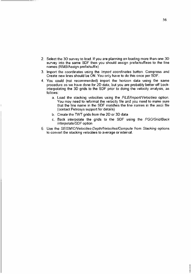
2. Select the 30 survey to load. If you are planning on loading more than one 30 survey into the same SDF then you should assign prefix/suffixes to the line names (RMB/Assign prefix/suffix)

3. Import the coordinates using the Import coordinates button. Compress and Create new lines should be ON. You only have to do this once per SDF.

4. You could (not recommended) import the horizon data using the same procedure as we ha·ve done for 2D data, but you are probably better off back­interpolating the 3D grids to the SOF prior to doing the velocity analysis, as follows:

a. Load the stacking 11elocities using the FILE/Import/Velocities option. You may need to reformat the 11elocity file and you need to make sure that the line name in the SOF matches the line names in the ascii file (contact Petrosys support for details)

b. Create the TINT grids from the 2D or 3D data c. Back interpolate the grids to the SDF using the PGC!Grid!Back

interpolate!SDF option

5. Use the SEISMICNelocities-DepthNelocitesiCompute from Stacking options to convert the stacking velocities to a11erage or interval.

57

Import the Well Data and QC Well data (header, directional survey and tops) is loaded into a Petrosys WDF as follows:

1. FILE/Import/Landmark/OW~ WDF

2. Create a new WDF: a. You must define the Units (and this should match the units in

Landmark) and the Coordinate Reference System (and this should also match the CRS in Landmark)

3. Select the OW project and the OW well list 4. Highlight the wells and formation tops to import

5. Import the well data:

a. Load Common well name b. Filter by Interpreter if appropriate

6. QC the data under MAPPING/Wells: a. Use the appropriate icons to display the well header and directional

survey data for the current welL Select the appropriate wells from the list of wells displayed in the bottom left hand corner.

b. Open up the tree widget for the current well or for the selected wells ! zones and display the data in a spreadsheet view. Check the BH I TH locations and see if they are correct.

c. See the training notes for more infom1ation on editing I viewing the well data in a WDF

58

Mapping Now that you have imported and QC'd the data you can start mapping:

1. MAPPING/lnteracb\'e

2. File/Preferences/Datum conversion -set the appropriate datum

3. If this is a new project with no existing mapsheets. then you will need to create a mapsheet:

a. Mapsheet/Create!Coordinate range

1. Use the SDF as the input data source, leave the template blank and set the coordinate type to Rectangulars

II. OK

b. Make sure that you select the coordinate reference system (CRS)

c. Change the min I max East/North as required (maybe round the numbers up and down).

d. Change the scale and other parameters as required

e. OK

4. If this is an existing project then you can select the appropriate mapsheet, using the Mapsheet/Se/ect option.

5. Display the seismic data as follows:

a. Display the seismic lines using the Display/Seismic/Lines and data option. Create selection files /line style files as required

b. Post the interpretation using the Display/Seismic/Ribbon maps option

6. Display the well locations using the Displayi'Nefls option

7. Display ply files created using the Display/Polygon option

8. Display the fault polygons using the Display/Faults option. If the fault polygons need editing use the Edit/Contours, Faults, Polygons option to do so. Only edit the fault polygons (not the contours, polygons)

9. Display the 3D surfaces using the Display!Grid!Colourfrll option

59

Grid the Data You can grid the well data, 2D interpretation and 3D surfaces; do arithmetic operations, handle faulted surfaces, tie the resulting grids to wells and merge grids together. This information is outlined in the Petrosys online help and training manuals and will not be repeated here. This section outlines 2 typical workflows:

• Gridding of 2D seismic data

• Re-Gridding of a 3D surface

Griddinq 2D Seismic Data

There are 3 questions to ask: 1. What is the AOI (Area of interest) of the grid - display data, select I create

mapsheet

2. What cell size to use - ·115 to 2/5 average spacing 3. What clipping to use if any - do you use a clipping distance or create a

clipping polygon using the Edit/Create single polygon option.

Use the following procedure: 1. Display the seismic lines and the interpretation as a ribbon map

2. If necessary create a smaller mapsheet around the area of interest using the Mapsheet!Create!Using mouse/EN option (this will be the AOI)

3. Use the distance-Measure icon to work out the average spacing between lines and select an appropriate cell size eg "115-1/3 average line spacing

4. If necessary, create a clipping polygon using the Edit/Create single polygon option. Save all the clipping polygons to one file (eg clipping.ply) and create polygons for each fom1ation. If you can get away with one polygon then that is great.

5. If necessary create selection files containing the wells and seismic lines to grid -not generally required.

6. Grid, Contour, Volumetrics 7. Grid/Create grid

a. Define the output grid, the input data, the fault file, clipping polygon etc. b. Important parameters include Cell size, Area of interest- mapsheet for

2D; Fault file - no to Z value; Contouring - 10 for faulted cells and contour up to faults set toY

8. Display the Grid I Contours on map:

a. Display/Grid/Co/ourfifl to display the grid - select an appropriate increment

b. Display/Contours c. Display/Co/our barto post the colour range

d. Edit/Gradient if you want to edit the gradient

e. Display/Map base to display the mapsheet on top of the grid

9. Display the grids in the 3D viewer

Gridding 3D Seismic Data 1 . Display the 3D survey outline on a map using the Display/Polygon option

2. Display the interpreted values using Display/Grid/Values and make sure: a. Symbols = Non-missing

b. Values= N This will display only the interpreted values I traces

60

3. If necessary, create a clipping polygon around the actual interpreted values using the Edd/Create single polygon option. OtherNise the resultant grid will cover the entire 3D survey outline Save all the clipping polygons to one file (eg clipping.ply) and create polygons for each formation. If you can get away with one polygon then that is great

4. Grid, Contour, Volumetrics

5. Grid/Create grid

a. Define the output grid, the input data (3D surface grid), the fault file, clipping polygon etc.

b. Set the AOI to the input grid

c. Set the Cell size to a multiple of the cell size of the original grid (or leave exactly the same)

d. Make sure Snap to cell size is set to N

e. Other parameters include -Fault file -no to Z value; Contouring- 10 for faulted cells and contour up to faults set to Y

6. Display the Grid I Contours on map:

f Display/Grid/Co/ourfi/1 to display the grid - select an appropriate increment

g. Display/Contours

h. Display/Co/our bar to post the colour range 1. Edit/Gradient if you want to edit the gradient

7. Display the grids in the 3D viewer

Fault Handling There are a number of ways to deal with fault polygons. The recommended approach is as follows:

1. Grid/Create grid and grid the data as described above, but make sure: a. Select the fault file

b. Set the Keep inside faults field under the Faults tab to N

This will create a grid with no data in the fault polygons

2. Re-grid the grid using the same cell size, and the AOI set to the grid, but do not include the fault file. This will result in the values in the "'fault polygons"

61

being interpolated between the existing grid values. Because the AOI matches the existing grid, nothing will change away from the faults. You can even use a different gridding method if so desired.

3. Load the fault file back into the new grid using the ../Grid/Load fault file option. This assumes that the fault plane between the top and bottom surfaces is linear. It will not work if you have listric faults (for example).

62

APPENDIX2

Increasing interpretation accuracy: A ne\v approach to interval velocity estin1ation

Hy 0.'11"/0 JIADL£1: JHF TIIORSU,\ "'"' -~11.-1.\·,vu,\ .IH/IL"R Sirrru Gt~I'IJIT.'·u·(.,, ,,,.

Stoultf,,, HiJ,·hi'IXI••Jt

A .:rudal par.Wo.\ <:'l:i"\1~ In tht ~t\CrtpaOL)' tx:r\\Ctn rht aocurat.'' to whu:h airl"nllimcs or seismic aTnts arc routincl}' pidcd h;· iallt."'fpn..1e•~ ta l"eo.e.• rcnrhs of a pcTCCn!) and the: a:.:cunacy inhcrcnr in 1ht' u~ nf inrcn•3J ,·elocili6 for dtp(h roa"'tr5JOn (10-20 per· ~r:nn. In i!ddrc!'sins thi~ fuil 10 000 [l('rccnr (or full (:J..:rur ''f IOI.It differcm."\" in r.ti."CUI'UC)', a new appmacb for vdociry dctcrrnin· arinn ha.o.; htt'n dL'"\'cln·('ed. This 3pJUoat:h ditt""i.'ll~ ndctres-...-s rhrt.:.· 1n01jor prnbiC'm~ rh.ar dqtadC' imc:r,·al vt"lodry .nnalysk compl6 fl'\.'trbutdt:n •Mu('{urc:; un<.-~Ulinl)' in rh< lot.:OitioOJ, slrH:(' and dip of thC' depth-point rdlrctor: and dcpth-poinl .lmt"ar aL.""ll'lg, rhL~ rc'IIC('tor.

ThC' nc'A' uppro;;u:h sn:atly lmpt"'\T~ upon tt:.--c indu.ur(:<~ wan­d:ud ILochnique~. T~rs :iih~· lh:u the d~ri\'t'd inu.-r,·al \'chx:ili("~·

dqt.Jn rrom rhe model ''doc:UiL-:s h~· :•bour I·~ ~r\"fnl in shaiJo~· horizom ~nd by 2-4 pcH:mL in th.: ~ hu.ri1on.\. Fur the Mt.ml"

nJ4,:M..Iel!> \.""l."~rnp.ult"d "'ith tht Di.~ equation or from the dip-collt'('fcd Oil" tqu:uintt'i (.sl.al~rct technaqut), ihe inttr\'21 '-'tl•xiti-e"' ,.ari~d by 20-~0 pc:nxnl. In addition,'~'" 1\a\'t s.ho\4n thar thC' aDJ'Ml)a..:h i~ ~~~bk i;a thl' pn .... ~·nt..'"t' of typical r.ois.: ln'('b 11.nd inlc-rprtlation unc("rl!lincic~.

Conct"PIUally. lht ll~ltrmination of inl~nal \'dt.:ily is a ~mph: ~eos"tltl:i.; problem. \\'i1h incK3:\ins off.Kt, rhe raypalh1 ~i1hir1 the intcn·al of inrtrest dla.nst p31h !cnalh, :md 1hc oW.c-ncd lrJ~>·t'ltimei show .J \:ba.rncCC'rislk mO't-cout. For geologic mode-ls "ilh t:(lfl~lttlll int(ro.CJI \'dOdli(S antJ sirnpk naf>l)ing in!<l'fat'C'. the ob~r-;.'Cd mO\eout is ~iriciml ro soi\~C (Of inrc-r\'ul \'Ciociti~. ronun:lld)", aplo1'31ion ph)~ are p:n<r.lll)· mu.."'h """"in=ling. and tunforrunateh·t ~imple a.s.~urn.ptiom can prO\~ ~·~full" intJdcquate FigurC' I :\h~:'i n !Ji.ghlly m(trc inrc-r~lin,!. 2-0 geologic mode-l and lht' schmk ro.ypa1hs 3ssol:iru:C'd wilh one ~flt'::tiOnl"\'t"ntth.:u L""Onlribule to I he L"tlmmun midpoint gathl'f_ AL.""Curatc roolurion of the- imcn-al \'C"Iocity for rhc Mnc irnmcdi­atd)• ;.~~bu\'(' lht' rcfk·ch.H rC'quirts an anal)'sis proccdart lhal u~.·eounu for lhe- compJ~.\ oo.-erbunk'n. the lo...~rion and dip of 1he tl:"ne~:wr and thL· d~.-pth-poinl smear.

'f'h< gC'ologi' O\'crburdcn can i:urodlk.-c un .. :mainty u.nd l"l)mpbiry in lwo Ji~in"; Wil)'~ ... lr5t,l;n("r.t) !llrucluml \'3ri<uions 3lrcr fi.:Jlh lcng1hs in an irn:s.ul~u f3!-hion rhal cannoc N eol:ciily pr-Nictcd from the bmk dat.a contained within a ringle gaahcr. Nt.."::il, the O\'C;burden m~· \:Onwin inre-n~l I!C'I<X:iti~ thai '·ary boih latc-raJI)' und vcnically. Clearly. lhe1C cffecB conspir .... co tk&radc rnolution of lh< componcr.t of the obKnC'd mtn'C'oul rh:u !i~oilld bfo :m:ibut~d to !he 1:uset inten·al.

l"he se-cond major probkm. lhr lr>JC' locilliun of the l'('n~cor. b 11Zu1icularl)· imponan• and diff...:ull. Pa1h ltngthSc in thccargct ini('J'"\'al arr di:l:\."tly dqlC'DdC'nl on I he position of thl1. rrne--=tor: hoWt\"('1. \\ithout a ,t:ood '~tima1e of 1he inler ... al \tiOOty \\(' t.'3Dil(lf t:<•rrccrl~· position I he rer1cc1Qr. It is:' bh like .s,a)ing 1ha1 11 \t-r)' good 3nal~·~i.\ of inrtn"OI \'Clociiy \.'Ould be prOI/idcd if 1ht- corr~:l ans'olt<J -.c-r~ u~ilablr 41 thr- ~inning of I he- an;ai)'!.i:>.

For srolo&K sUUclurr:s oaith dip, dthC'r .ill tht t.uaeE horizon '"" in I he 1}\'Cfbur~-n. 1~ f.'ff«J:o> ()f dcp~h-p0in15~ar can funt~r comrlicaie analysis. ,-\s seen in Figure I. I he l.ar off.~cts rrod rn

Thi.) pa~r "'·u_,. pn:~rtt«i bifon.• th~ GnJph)-sit:t~l SO<'N'•'Y ,~( llott.Ul)n, JanuurJt' Ill. 19M.

rr:ltt\.'1 ;rum~ \IKtJIO\itl'l pomon or' ftu: dipping ftOcclor. 1hu ... o:hangin_g lX11h lcng.th:-. from rhc.\C "f rhe: ideal Cil!'oe' \A'hh a s-ingle r.:tk\."tion poin:..

l'hc pn-via-.HJS o~'"' \'at ion~ may plo,·ide ..... )lllt" insi~hl inro -..·hy rtu· ~~o:~olnrinn ~1f inlct\•al \'dod"· ha.~ rem.lincd onC' of the more dusl"~ probl--n't:i "--onl'romt"8 -<b.;..~e depth ,;:oom'C'I"3ion. Jt sh..,._dd nor t\c.~ h.NI ~urrrisine 10 l:Ond1Jde rh3r a 5-.111\facrory .\olulilm ri.'l..llrirc~ i"lrini!iRL! to bear t"\l:'r)' bil of lnformation il~-ail;sbk lo 1 ht' intc·qnt1C'r: CM P ~·ubn:o., cime ma~ o\nd :u:cur:ttt .esrimutcs ()f I hi:' O\·ethur'd.;"ll \'CIOL'it~· ~lfliCIIUC.

Fisw(· ~ prrwidc~ a £raphic ml:'n'iC\4· of il mtlhod rhal O\"t'r· ..:t:-~nc\ the prublr:tnl di~"'U~d. lbr darit~ the- method i!l pre,.~nh!d ;~,,a ~-U ••naty~i .... hur rhe mcrt\od i .. cqu:tl1y ap11IW:able to ).f)

lt,L"<\rnt:tri"''· For a~~ttmcnl's sake. ass11me I hal Hudzons I and 2 1Figu1c 1A) h~\.'t' alre;.uJr l~n dtpth .::on"\"tllct.i lfi~rutt l.ll) and ~ha: tht• l;•'k j, th.: c~,.-..mptllalion of the imcr .. ·31 \'C"Iod1y ht~: ,n-.,.•n Hori;~.on' 2 and .l The argumcrll remains unchanJed lor <~ny number of tnt~r\·ab. indoJdin11he ~impk- first inH.•nal.

For ru1~· ~iawn c1long tht" zt'fl'·Off~ s«"li,m. ~Kh a~ l01..'"3tion A. rhe 'l''r"'t" of th<r. rim<r. pid: ..:11n he used ro ~omputc rt-.c dircc1ion 1ha1 S(btntic cn::rg)· appruill:hed th~ C'Mf• (.;,:ornbina· lion vr ttk.- :oi!of-1( or Opp:;trenl \'Ciocil)', Snell's lil\t>" 31\d lh~ surfacC' ''docicy :u )'loim .'\). Ttl€ se-ismic ray thm can be '-hOI into 1hc .:ar1h n1odcl, rcfr3.:1ing :u cncb il11crfacc aK:ountcrr-d. Whro the ril)· n=ach~ 1M bl.'ttom of lh( model, tbm: i\ a bil of 3 probk-m­tllt' ''"·luc.:iry i., •h"'~l ~'t:t lr;.nn..,.·n forth~ nnl in:tr\'D.I. Ha-C'"\'I:"f, ll.'t

wilh .:onvrnuonal ~tricking \'t"locily anal)lh. th-ere i~ :!100\t> ~t"t•lotlcally IC'a\unablc ran~ I hill ~hould be scanned. For each wk_,.,_.icy in th~ ~c:ul, lht r3ypa1h can bc extended through I he bonomof a he model until thC' total path lcOith corrt.\llOnd!- to the obscn:a:d 113\"t:llim~ from the section.

tn gi..'tlc•al, IC.lf the minin1um \'dociry I here \\ill bC' a minimum r<fra.."1ion unglc and a )hallow rt'nC'C"Iicln pOinr tpoinl Ron Figur~ lUJ. SinriJ:trly. the highest "cloci1r '"ill, in general, be a,.(ociaicd wi1h I he large~• 1d'ractioa angle iU\d the dc'Cpe~ rrllc.:ti.on poinl (roinr Con F't~urc 28). Hcno:C'. br !1-L-annins a r.~nge of ''dociries of interest. !he location of lht renc ... ~tion deplh p('lilll can bl.' \::..nnpul~o"<l. lhus p:tnially ma-cornlnJ I he sa:o-nd nH~jor problC'm of d\."1,!-ruding ,.C'Ioci1y anal)~i~.

E~o.11ma1ior. tlf rhc rclle\."'lion dcptb point !) unl) tt~J! llf lh< solution. Tile local shop~. oral least 1he dip, of th.;o 1eflCL'hH in rhe \'icinil>· or rh~ renection poin1 must br rstitnatcc:t H~·l'f. if the .w:Wnk K'l1ion bring analyzed correspond~ 10 ~tacked da13 (i.e,., ru.u riml" migrated •. 1bcn lbC' rcOmor at depth mu!!-1 be' pcrpendiculur 10 lhr normal incidence r;l)'f11lh asso:i3Eed wirh C'ach trial \'dodly, Thu;, for each tri.al inteJ"\"31 vc:locit)·. a trial plauar 1cfle~:1or (Don Figure lB) may b( incorpornttd into the model. normal to the a:"'sOI.:iatcd raypath and pa~~.~·ina 1hro-ug.h rht currespcmdmu depch pOint.

t-inaU~~ 1hr Ja)'palh."\ and .a.!lwdatrd lra\'cltimo th;,t~:unn~-.:1 .... ach ~""lUr..:t-rccdver palr ~·ilhin a CMP g:nhoe:r a.nd 1h.a1 rdl<:c1 from rh• dippina j>l.lnt e.u be comP'.rtcd (figure 2Bllly Rpo:atina rhls: rrn:rs!' tor a!"~$ of \'C'lOt..ilin.. a family of lr~\.'l.timC\ ..a~u~ ort~et \.'"Uf"\OC!I c Figun: 2C • can be computed. The cur~ .orr fully c.•••rr\.'\:ted lnr a!l of the crfo.."'.\ of 0\IC'fburdm !l'lruclu..-e otnd \lt:locil)', lo-.·atiL'n ul' 1tre dcplh point and the loa! I dip of ahr reflector.

GEOPHl'SIC~. TI-ll l.t:AIJI:-.t<; £L>GE OF F.XPI.ORATION SEPrEMBER 1911~ IJ

;\!,,,L. 1h;1t •••~·""' ,_.,,r,r.-. :u(,', in ,tet:lh..'t~l. nunhypctbol• .. :. •\., a rin:tl '\h.'J), lht• IUIIthyperboli~o.· lllO\'l'OUI o;.:UI\0 OIU:o-1 tx'

~1HHbint.'J ~ilh rhr f'MP g<~lher..; w sda·1 till~ f'>i.::;t ..:·:;rinJ:~h~ 1.11

•ht.· intt"n~tl h'l-tl\:ity. 'fhi .... i~ u fairl)· ens~· rns\;; lht• wmpuh.~d JliiiWl'IUI ~·azru .. "' :!n• idt.~lly ~uitccJ (or ~t.acldn8 lhc gathe-r,, ~ . .-umputing "~mhl.ancc and as~c....,~fng whkh CIU"'r orttimizc, rht' PU'\-'-'' iu 1h1.· sh1d. Th.;,· simpJc: Ktcnlitii:Oltion i ... made- rh~t rh~· ~'llf\'L' \\'hi,;h (lplinlii'L"~ tflt' Sl;h:l ..;I.,HI~5-pOnd-. lV the \~-ltnl'\.'1 :J\'<TdF.L' illk'n·al n .. k ... dl~ fnr lhr /llf1l.· abtl\'L' the- dl'plh-puinl c.\lim~U< (pttinr D nn Figuzc 2HL

hnplt.·m .. ·nt:lli\)11 oi rhi~ <"ipprva~o.·h ~"t'llllirc~~ a IC'\\o· adU:ition;JI LomidcrJti, ... n_,._ Although 1h~ ~mcrrue1cr L"'.:tn Jlrrt\'iM. :ttime pi.~L 1.11 lirnt.• map (or ...-~!irru.Jting chc- reflection poinl, in pmt:tk.l: thc:-rc­"-'ill ulwa)'l b<." ~:Sit' URl'l.Ttu.int)· in the absolute reliability of the trm""- Wt:t~ lb~ pe:ll.:.;;;, 1 u)ug:h,\. or i'<l'r!'l cwssin;g.'i pt._;;kt'LI'~ \\1:\!o- lh< nup .~m,~mhL-d or t.-di1C1.1 in some "·ay rhar 1113)' inlrCidthY rninf'IJ but ~ig.nifKant errors-'!

Tht ~olurion w th's prqblt:lfl i.) ~ir11ply 10 S..."'..ln ~~rang( of timt'.!­IS3)' ± 150 nu) around !he pic~ rim(' .and compute- a ran,gt' ol largt'l tt'11c:-~..:ti<.tn pltint~ and iUMJciaLt"'d mo,·~;.·uut -rur''e.) for ~ad1 ~ciodry ar each iim~. Rnally. 1hc 5cmbl:m~e -can be compuicd f.:.u c-a.,;.·h rr.tJ\.•roul curve as a function of pick tim~ and U'l-'t'r.t,(' ill1~r'-·al ·-·~locily. A~ might be ~,pe.::tl!'d, 1h-c rt:~ylrtt...-ins ,-on)umc~ u rrl;tjm i1r o1

tht· CPU tim~ in this app11.xu:h. Widlll-UI cart"ful implcm~rualkm. o~ t"ooh.l find thai I he- L"'illPUiatiuo of :t~C'\-eral hundred rlll"'-'c.."'t.Jt cun·('~. oouc~ponding 10 c-.1o:h .. -do..:ily-timc- p~tir. •·ould re-nder rht.5. 3iltacliv~ a.p~:-03Cb unfcasihlt. E\petitnce ha~ sbtl\nl th31 1hcy gcncraiJ)' .::hangc shape rather prcdklahly wirh dlangc-.; m tra·~,:c-llimc- and inletva) lfdodry.

Comptu::uion llf about IS cur H ..... , ~01 r~r,::mding 10 1wo Ill thrtt if'3\:dlime-s ,.-mtcrtd :.round th( pi-=k tim(', and Ji,t" to St"\'('f'l

\C~hie! spannin~t chc ran.sc of int<"ft·s~:, is usuall)' ~uflicicne 1n

dc.~~ribc rhc bchn\'ior of lhc m01o.·cou! cur.n 11~ fu:1cliom ol pkk tirn\.' and interval ,-elo~:ity. ·rhis ,s:ct of mo,·~out ~o.·ur"'l"l ..-an then h.;.· intl"IJ)OI:Ut.."<l 1u a mOll.!' t.l<:n~c- :.cl, as funl'1inns of timt.." 3nd \c-lo.:il)', to obtain hls,hcr rc:soluti-on lOr picldfl!!. !oenlblan.;,:c peak,.,

Thll:' ~JBorithm "'3l:C!Irhc r-... plicir !l.\'iUmp-1ion th.ul the: over­burden s1ru.:turc. in lc:rms of tntvdlimc- c-f(c:C1!rt-, i:o. kn()tll.·n. Thi!> n:-quircmcnl can be- met if lh(' "·~10\:'il)' al_torirhnl is u~cd whh a m.ap mis,1a1ion al;orirhrn rhar al~ accounu t'or tht' oo.-cr­burdtn. The depth con\·enion procc-S.\ is tbrn '"top-do~A·n, •• ~·hich is as follo•·o;.: Fir.u th(' ntar-s.url':ll'C '-'t:r•-,dlit':) are dl'fi\'td (staninx model ha'i no horilon~)- Ne'U the sh.all~-c~l u-a-..dtirm­map is mignucd to dcp<h. For m.orinc pru .. ,llCCl~. rhc procc:s!i starts ,.·ith the:- finl layet de-fined h)' tht ~e!ocit~· of water and the bathymetry map. The ""locioy al~orithm istbtn US<d towlw io• fhe next dcc-~t in1cr\.'al Yclocit)· .. 4Dd the misration routine u~e!l thi~ ckrh-c:d ._-efodty mop (OJ d-eplh cOn\~lsion of lhc n~t cJccpesl l/"3\'t'hlme- horizon. ltlis pro..:c-!1-s is rt"f1C'3.Ic:d umil an timt' hOfilons h:t\'L' bt't-n (un••encd (o d:pth.

Ra:ure J ~how:~ a ~omniem layout for plnt>rHiug hJ th<- illl(f· prctet the rtsulu of the intcn·aJ ~'f..'hx"iry onal)·.5-i.s for a sin,slc CMP gar her. On rhe !dl il< the ~Cmblance plol s~r<»ins rJw, roower in the sanbla.ncc sp.."Ctrum Olio a funC'Iion of pic~ rime- and ;r,nagc int4.-"tWd ~rt:1ocicy. Note lho:t the- spo:trum is r~ winduwtd around tht pick time, which is indjcatcd by I hit' bold hOf'izontaltkk at 2.125 s. A •-clocity pid •)f ~1880 mi.~. indicated by the 'ortlcal ban on thll:' \'(IO(ity a.\i~, has httn madt by rhe intcrp~t(r. ·rhc !1-ei~mi~ gather hns been fllutt'ncd us1n.g th~ cumplc:-. mDVoour OJ(\.(' appropriatt ror I he im~:rval \'t!tt'tciry-rirn! r..ic:k. as docriba.J. B\' pj<killtl •ario~ '"locit)'·rimr pair.< and rafupl<ryiJl!llh•ta'lhcr with rhc approprinlt movrout cur"~ 1he inlapreter ean quicld!-' asso.! ae<.-uraq~ ln.aflllropri:ue- \-do:irie-.s will do a poor job ftt'

O::.rtetting the t\•tt.L The fl<IUtnl."'d •ather h& bl"'eff summed itl

prodocc- ~ ·•zcro·off$~1" ua~.-x:, -.·hich is d.is.playcd in 1~ cc-nler of lh~ figutT_

63

llh· "1111\tii\'U (Ia .. ~· f~ri,,,IUL':'o :..i '-'l)I\'•CUh!llll\.'(~•ft'fl..:'-' till .:c·orft··

l.:tllng 1l11· t"\('nt .unv~l time ~-irh inr .. ·rT~tl H"IO(ity. The- ~ath!:r

"'"'~"'·nun FigiiH' 1 ..,-~'-" a~!rt-•.K"i~tc-11 l.\'f•h :1 \(I\ "'''Dil,t \'('ln..;il'\' flt.";lt. tho1: ..,.;,, "'C'II .-nrrd:UL"ll .,.-irh 1111.· pidl."d. !:\-~Ill. -Hr,.._n...,.....;, d\;'r 11nt~ poniu1\ .-:1 ;h," pl:tY. b•)und~·d hy rv.·,") gro.,.,·rh fauiB. it

:u ll·n••.t.= •a\•~rtrt:•··

~-- ,, ,. ~.s ... ~~ .. ~ n ,.., ; I J

--;;. •.. _ ....

: :.C•

'" .. (

Haurr 1. li'111odtlmn on a CMP g.1Ubrt in stradt~n.D) intnn.ti~ ....,., ,._ • .,, I» prodkled b)·lbr simp6stir Db not·lll)tr .,o<IPI.

A.

T I

M e

l B.

D E p T H

l

INTERVAL VELOCITY ANALYSIS AND

THE COMPUTAnON OF NOH-HYBERBOUC MOVEOUT CURVES

-· DISTANCE-

OFFSET­C.~--~~~==~

T I M e

i

TUtli•l,

Fi~un l. lbJk r~o .. ..,., of olw otocbl-b:a...t ul<>cil) nllmorioa olgorilbm lOt' olaR)r CMP •••rb>b.

14 GEOPH \'SICS: THE UAt)I.-.G EOC.E Of CXPU>R.~110N ~EPTEMBF.R 19!11

64

fic•ft 3. RtMtt of tiM •ten~~ \1411eclty aftllrslt f• a lillie CMP ptlltr.

was notlted that the vclocity peale and the intcrprrtcd pick times differed by about 15-40 m" R.ccxamination of the scctiOII$

uattd that the in~e~pm~ had sltippcd a cycle ~ thi$ ponion of the map. The joint pracntat:ion of the stackrd lrHe and the ~"Ciodty 5J)CCtnUn provides • sood mcc:b.anism for the iatqration of event pkkina and intft'pl'dallon with velocity aoal~

The stacted trace is also ext randy impol'tant for mainlainina consistency between the depth c:omnsion (map mi.,mlon) proc:as and lbc solution for intc'WI \l'doc:itica. A rea:n1 test .Ub dau fi'OIJI the NOfth SQ prc:wided an int.cteSiina example. The sections c:ont.aioed strona refkc:tcd a"mts with a ~let shape that ~lied tO be a doublet (I.e., IWO distloc:t renections that "'Cl"e closdy $J)IIOCd), ~ thou,Jh the 'lediom had bam proclCf.ICil with deconvolution opaators. ~ atlben wue aoalyted and displl)td ln the format

lhown in Fiaure 3. Each ditptay bowed two dosely &paced \I'Cloc:ily peala associlled wi'b the doubld; the lat~ velocity pealt was always assorD&rd with an intcnal vdodty thlllwas S')Wmati­cally lo.er than r.br rwt peat by about 4-6 percent. The se<ond aemblaoce peak was interpreted u a J)CJ·Ift multiple from a sMJJow low·\ICiocity moe lhlt reclucod the dcrMd intawl vdocity estimate by the: contribution from the lower ~locily pq-lq path. J\&ain, tht joint di play of the velocity analysi5 and the Jlaeked tn1ce ~ a powerl'ul tombiution for hiah·resolulion veloc:ity lllllllysas. Jf the vclodty ~~had avcnpd the ICil\blance oYer the lime pte of the doublet, the interval veloclly mapt would

have been systematically biased toward low ~•lues, and the depth miantlon ~'OIIId have undm:saimatcd the true depth <>f the target horizon.

A. noted. the propo&ed al•orithm is at()JH~own procn.'l that cycles bet~ w:lodty cstim..tion and. map mipation. lr 1s UD.,ort.ant to note that seiunk noise will add anc:crtalnty 10th~ \'docity llJSal)Sk of CMP pthen. and rime maps usually rellect boeh liard dau and interpretation judaement. The final seolgic model is developed in a series of steps that pi'OCI:ed from the sha!JoweM horiwn to the dcepac. Obvious questiofu arUe: What haPJICIIS when .some error is made In the shallow stroctun1 Docs !be aJaoritbm diverp 10 llll.lotable or unreliable depth estjmates'?

Asimplr JCO~ araument allows that the ptOCC:SS i$some>­wlw self-correctina for the U$U&I uncertainties and noise Je\.el~ typically encountered; however, the method cannot compensate form~ interpretation blunders. CorWder the a.sc: In which the Interval Ydodty bas been llllllerrsthnal. The depth COllYer·

sion process wiD then underestimate the true depth of the associated ~llcctor. HOWCYCr, ttle m<MOut informatioo coowncd wit.in the prhm mn.UU unclwl.,cd. Telardleu or the derived model. and conuob the selection of the "01)Citnum" interval velodty. He.ncc, the interval velocity analysis for the nat deeper zone miHt au.tomatically ~lcc:t a ~oclty that 11 sllahtly biaher thaa the true inten-al ~etocity to compensate for the error in the Ollefburden. Oepch conversion U$inJ the dmwd ~will

GEOPHYSICS; THE UADJNO EOOE OF E~ON SEPT£MB£1t t9U IS

then produ~ an iot~ that is sliahtly too thick, compensaM, for the error in the 0\'erburlkn.

This aeometrical araum~t has been checked vrlth 5eYffaJ synthetic modd data seis ia whkh tarae ~~elociry variations were "htddm" in tbe anal)'Jls. These models typically conl&ined f"n1: to scYen horizons. The coal of tbe~ tests was to stmulate tht! real.-orld case~ here sianirlc:ant Yelodty Vllrlatlons m~&l\1 occw -..;thin an 0\l:rburdm sci$mic 5equenoe that was not mapped and, hence. not captured in t~ 'll:IODt)' analysis~cptb com-enion process. The resulu of these tests w-tre both surprisina and cncouraaina: the: derived interval Yelocitles lkpanod from the model \"elocit~ by about I 2 percent in the shallow horizons and 2-<t percent in the deep horizoll$. Rlr the: wnc: models. inta'Val ~lcxuin computed from the Dill equation or from the dtp­corrccted Olx equation varied by 20-50 pc'I'I.TDI.

The ataomhm is a top..down approach that intearates wtcb the depth convcr ion of each mapped horizon and is used to ttnl estt!llilte the ~'&! Ydocity of the shallowal horizon. Map mi,aration l~ next u~od to depth convert the li13ot time map. The derived overburden strueture is used, in co11junc:rion with the nrxt deeprst time map and the Cl\.fP prhen. to estimate the tnten-al velocity for the S«Ond horizon. This pi'CK'CII continue$, alternauns between lntWt'lll vtiOI.'ity analysis and depch COII\'ef· sion, until all time map. have been depth converted

This approach sianiftcantly increases ac:c:uracy when worliina ""ith interval veloc:itieJ. And hccau.o;c it also reduces the: time: s~nt on suc:b estamatn, d as c:ost-cffec:tive. ll

Dovld M. Had/tJ is# rofoulldtr of Stm'O ~physic$ llttd lias ~n'ftl QJ stftior ~ praitknt since 1~ comptmy's ~,rinntn,r (1971). HISCIITI'f!lll rrsptNWbdllils illdudt dir«flnl all rr:starcll and so/twtut product tk~'tlopmtnt. PriOr to foulldmg S~rra, H(l(//fy ~t'QS t1 ftfNI'fh /tlluw fl/ C alifomw lmtitut~ of TkJ111oloty. H~ ~YCti~td 11

docton1tr in~ from ClllT«h lind tl mtr$1~'1111 ~fJ/tn10/rom the u"'~

!lily of Ctllijornill. Ri~wside.

.Jtff Thorson is 11 StlftOI' :miff r«Jphyskist at StrTTII Grophysia. &Jon JOtllllll tht firm, II# worJctd as fill int~prrtlll tOll lto­pltysiciSI in rllt llltt"'attonal Dl'lli.sion Q/ GttiJ Oil in Los An~ts. Wllilt .,.'Ofkillt 011 11 doctOfGit ill g«Jf)hysics from Sttmfonl Unt~IY (/914), ThorstHr did bask ftSNrr::lt ill J("U1111(' ~liS II tnmJ1¥r qf tlw iNhalry-spoiiSOI'«i SJfll1/ofd ~:;xp~or. fltiOfl Pro.i«t Ht rrc~Vfd ollS. irr ,oiov

from tilt Uni~'flnrity of Washin,rton (197JJ Mid 11 M.S. ;, lftJfJ/IJ. K&/rom tilt Untrtnlly Q/ llouston (197$).

Colorfldo 11981}.

ShtmnOif Mflltu is SM.ior -mr mt1~ 111 S1trnr Gtopltyrla wlat~ Ire- IS rnpon· stblt for mtmfl~mtnt of tltt rompafl)''s forwllnl 11ttd inHrst modtlin1 t./ftNts.. Pnor to ha aurmt posttio11. lit t110rktd f~ the USGS. twtri Q{ Pwrop~ tllld Rrmotr ~lf.Sint (1979-11}. Maltrr Hrn«i 11 B.S. in rl«trklll rnrinnr1111 and com­puter scitllcn from M I.T (1911) flftd Off

M-"- in popltysiajrom tM Unt'HrSilyof

16 OEOPHYSICS: 1HE LI:.AUtNO EOOE Of' EXPt.OllATION SEP'TEMaER t911

65

66

APPENDIX3

Interval velocity estimation using iterative prestack depth migration

in the constant angle domain

Bl .\: D rrJ-.:InJOR£ Olld J D. G .... RIYG -~1110(0 Pl'<xh.crion Compa11)

Tulsa ~alwma

T hl5 article ru>rus;es a rechmq.:e wl:tch a Clllllber of peop~ ar Amoco ha\·e been wt'rkm2 cc since C:e eJI}\' :981);

\\'e begm by anm~r.g n\"0 que-;:ioi:S rn:"a; i: tiw COII­

STOIIT tmgle domain .' and rn..,· would m1_lone \\am ro r.:e ir" ftr>:. a::hcu~ the cooc~ ha; been zrou:::.d for dr better

pan of two decades. :he :e.'1ll ··coltlam mgle" 1-; no: widely koo\'-U (:br e_v.ample. :: ~ oot :nc:uded hl SEG's Errc;~daJXdrc Draionar. of Erplo1 anon Gr,epin·:im p;obablv because >tlmUC e:tplt'raUon has tndiUt'113ll}" t:sed a point source wbio:h geuera:e--; rays in ~ direction~. The cons:allt angle :echmqu.e. or. :he other lund. use> m e.'t:ended. =~ which produces a plane waw that has a smgle ray parallll!:er along Its enttre lenitb..

Thi; n na: 'U5t a marbe:n:J:ical eo&\-emence. lt COU:d be doce in ~e aeid. . .i.moco ac:ually perfonned mch an expen­:n:mr in che i.a:e 19"0s b<,· mnclraneous.J.y 1~11!! a >enes of sat:rce'l Bur. of cour;e: such fteld \t'Or:l: ~ camlo: be done routme:y because it'; fur too expen;t\·e. Howe".-er. coustan.t angle da:a can be produced \\ith corupn-..er> by 5t.tperpcxdon of a ~enes ofpomt socrces initiated s~n:i.al.ly\\1-:h a ~ar

Figun 1. Fonniog a btamtd plaM wan.

nme delay (F1gure 1). Se-cond. the ma•t'r reason :o u~e tlu; do= 1; thlt it can

handle a large ime of imagmg a:gon:ht:l~. frt'm ~ct !UO\'eou! t'n thr :ow end :o full f-x n:lgl'3'lcn at :he high ~d. There are wavs to actu.Jll.v do e::asric n:ie:raoon mth I'll\'

prect;ion. For the most pa..-L' tlus i; the oU:y do:nam where all :hese a:..:orirh:us e.'Cls:. Their a\'31l.:lbilir.· n:Jl:es :his domain sui-.a.ble ~for mi2:1.no~:c \-elocr:y an.'llv:;,s becwse t: allows the use o~nry fa~t~f-1> n:ethod>. P:....ase Sluft ou~tions, Ki"'Chhof t:ll~Ut'US when ::ncre co::np:.tc:~:ed mtdu :u-e encOUil:et-ed. :md. then f-x ruJgrat~om to ha!:.dle 100:-e arbimuy m..adi.:J where :he Kirchhoff a:e:ori:btus start to break do\\U In add! :ion. thi; dore.1in allows the u;;e of uxen.U \·eloct;,.· mode!; \\illch are c.o1 bol:nd by a>rumpo.ons o: a horu:ot:ta::y $tr.llcled eanh or by the = approxnr.anon.

Cocs:.:m: ~ prestad: proce;;mg require; two maJor ~eps: 1) coi:St.m: mgle plane \\'01\'e ;ynthe-;ts l.'.nd ~) JteroU\-e

C«l.S:ml: ang!t d~th llll~:ion. The fim ts aclue'\-ed by a mu-p traus!'orm of ;:o:nruoo

receh-e: ~1-;mogr.uus. :ollowed by a sort lll10 li~ ray pa-

t~tUQI..,._ tlli'Yf:t rt "'-'l Win 1~ ,....._.. J<~Y~t .. .,... •~""mrr

Fi;urt 1. Wologir modtl shoniaJ (Omp~doll:l! ~nn inttn-:tl nlocirits.

Figun• J. Constant angle time ~ections.

0 •

figut·e .t Coosrmt aoglt dtptb migrartd ~ections.

~5S TEE LEADIJ\G EOOE f~lY :m

67

0 I

Figw~ ~. \'utica! smck of dtpth migr:utd common :m­gles.

----' ....._ ~

.:(

--~-

.... ~ ..

'• f/l! I -...,...._ ·~-

..... /!11. -·

Fagw·t 6. Pt~tack mip·:~tion qu.ali~· contt•ol g<lthuo;,

STAC:I\ S

Figau 8. \ 'tloo~· ittrations for lartr 2.

68

ramete< ccll5!allt allEle eathers. The rau-p transform ~~ per­formed m :he f-x d(;matil and the re;ult 1s then 1J3nsfotmed bad; to :ime.

To demo::.~:ro:e chts. comider the model m ftgtl:'e 1. A senes of fuute-differ~e :ib.o::'Dotn.I "'nme:ics was p:oce;;ed to produce the cotman: ang:e • >ei'iiDOgrnms ih:mn in Filll!e 3 !\ore thlt exh of t!lt'..e con.;tact angle sa;mograms illwnin:ues a d!fferent pomcu of dJ.e substafuce.

I: a sunplt lwear de:ay ts applied to ea6 trace :n a ccns:an: anl!!e seis==. dJ.e reo;ul:in'l set:;mogrnm can be con>~.d­ered as ±e S~ece Wa\-efie}d re;ponse due !0 a plane '\\11\'l' source ;pannmg :he leu.,gth of :he line and as a cc~uence. a \'ilnety o: deplh n:lgl'3:ion algonthms can be applied to the dlta. In tbi:; ca;e. f-x diY.\m\-a::d contmu;mon opera:or; we:-e applied to produce tee cons:an: an,gle dep:h migrn:ion Sl'ls­~mgran:; sbo\m m Ftgure ~ Agruo. each tl:'wr:nu:e; a por­ttoa cf the substrl'ace aDd tlu~ir st:d: (F :gure 5 tendm a good

Figw-t 7, \'(z) po>tstac:k dtptb migration.

0 C GATHERS

noo t.1's

:.!60U MIS

lUO MIS

n::.y 1m

a:pproxnn:don of the ~a!tlll2 n.wl So. dus ~e---Jmique p-odl~s an oUiput SUl1!Z: to that of

cOil\".?lllional nugranon. :t ad\"at:tages are 1h3t a larger muu­ber of Cllgnttlon alg\Y.ltbns an anilable md that t: ~·es cOL.Sl~--able ··tenrage·· for \·t.:octty analy!;t; ThJt le\-erage ts :he ab1:1:v to piJJt>omt correc: \·e:ocmes on the const;­~nc\'-Of lack of cun:aru:e-of me d.1:a across a coust:u:t ~:e secnon.

riguR 6 ts an e.'taruple: cote tll:!t slow nlocttles cun;e upward (or ··;lllll.e') across the t·eloctty gather. :a;~ \-eloci:ies CUl"'.-e do\mward { fro;m"). and cor.ec: \-elocities are coc­~ta&t accoss ihe eunre gather.

69

\\"e h;n-e used :h:s !e\·erage to d~.--elo:p a teclmique for m:er..-al velocny de:ermina:ion thJt could be teilllied ·-pre­s:acl: la)·er stnppmg:· It can be tmplemeu.ted as foilows:

1) ~~e an i:::uw estm:1te :or thr u:.remll vt.:octtY and gradlents in !be 5rst :ayered sequecce. ·

:!) Prestack :ni!!l11te me con>te.n.t am:e dat.l dmm to a ~.dkieu: dep1h :o encompm :he \--eioci!y model in np ~.

3) ln;pec: tl:e pre,tack son and = to detel'lll!ne the \iJb1li:\" of t:be t·elocll\" es::im..1:e

-l) I? the es::imate r;'u:.comct. penurb ±e model approp:-t­ate:y :md rerum to step!.

LAYER SOLVED Entire

Model S t •LOilU Tlmd Fourth

Figure 9 \"elod~· model e\·olurion stack changts.

... :--1 I .. 1 ~

... . ......... -· ~

·-.

. - ---. -~

l•l f I I 1 I ' ; I; -· . I' ' . ,.

I I I I I I ....

~. -.. , . ... :;... , ,

Flgur~ 10. Pnstack d~plh mi . . . gtanon usmg lanl' stripp· r· · mg (Y.:J modtl.

Figurt ll. Pomtack d rh . . . tp oug.ranon unng pl~tack f"(x~:J modtl.

..

t I

..

I I

I I I

I I I ~ t l I

Jl:LY l9S3

70

.tlU U

1 11. 1

JStlil ''

JSJO . <

4.; ... ~. J

I ~I

:HE LE.IDIKG EDGE '51

5) \Vhrn ~ \"elocil'l· e~tim:J:e is corroct. e.'<trnd tbt tmtr. val \·elocity l!lld <rradiem estim:Jt., w the ntxt Ioyer and mum to'>tep1. · ~ ·

The accuracy and ndvan;:,ges of <his method con be illUStrated by e<>llljl3rison \\ ith a e<>m·tntioll3.! slllCk on a re•l data eJ<.1Diple.

fi_gure 7 shows a ronventionol po><stnck migrnrion of a salt conlllo=mrr. There is a hieb in the sands below tbt ~•h l!lld it g""=te.~ ~key cr.ttstioii: Is rltiJ jusrve!«i~·· p::llup m· U fi srrucrure?

This is difficult, if nO! impossible to determint. from Fi!!llre 7. Let us see if tbe 311SWtr is denrer in ilie const.mt ruigie domain \\tth in1e1val velociti., iternti\'l'ly determined from the top d<mmvard

We l1lD\Y the top layer is water and is flat at thr sUifuce. so we put that m l!lld continne to tbt second layer. figure 8 shows .some of ~ iterations for ~ .second laver nhere ~ ;'smile/frm\:n ver:ruc:; ftai'· criterion impli~ a cOrrect \'elocicy of2600m/~.;_

Tne ~olutions of~ \oelociry model nre ;bo-,m in Figure 9. figure I 0 sho'"' the pr.stock deptb migration usin_g tbt ,·eioc ity model deffi·ed from the cons mot c.ngle la)'l'r strip­ping technique l!lld Figure ! I ihows tbt posmack depth mi<rration ba.-..,d on tbt inrm'3l v<iocitie.s obtained from tbe pre$mck \'l'locity model.

In both Figuf. 10 l!lld Figure I L most of thr high undtr

i61 TEE LEADING EDGE JUl. Y 1991

71

the salt that wos present in Figure 7 bas vaniihed There is no do.rure htre .>e the decision was made nor to proceed in this arn.

As this orticle demon';!fotes, this "PPro•ch has pro\oed \iob~ \\ith both modell!lld reol dam. The cost is dependelll on the a.le:oriilim u.-..,d and tbe number of ittrations required if simpletri:ll and error is u.<ed o; eoch ><age, the lllll!lber of irrrntions c:m become large ond tbt proc.ss rrdiaus. How­ever, the =ber of ittrations can be reduced by inserting • velocity e<timation .step at eoch iteration. The velocity esti­mation S!i!p i~ generally based on a. resid.u:tl correction io the depth migrated dow..

Multipl.,, out-of-plane events from three-ditntnsional srmcrure;. l!lld poor signal-to-noise ratio ba\'1' all been found to complicate the proc.,s. On tbe othtr b.Uid the efficieJCy of the method is g=lly improved when a knowledgeable interpreter helps perform ilie iterntion process.

SugEeHions for furt:OO' reading. Constmt ruiglt p~s­ine: o1 sei'illlic d1"w has been discussed by monv outhors. The r.f~omt titles can be found in Rick Ottolini's.i Tau-p bibli­ogt·aphy (Sr.:mford E"Ploration Project Repon ~5 L1987).E

.-ic.l:nowledgmrmz: I wish ro thank Larry Lint'! for encourag­ing me ro submir Ihi.z papn-.