Minimizing the Average Distance to a Closest Leaf in a

[11:40 13/8/2013 Sysbio-syt044.tex] Page: 1 1–13

Syst. Biol. 0(0):1–13, 2013© The Author(s) 2013. Published by Oxford University Press, on behalf of the Society of Systematic Biologists. All rights reserved.For Permissions, please email: [email protected]:10.1093/sysbio/syt044

Minimizing the Average Distance to a Closest Leaf in a Phylogenetic Tree

FREDERICK A. MATSEN IV∗, AARON GALLAGHER, AND CONNOR O. MCCOY

Program in Computational Biology, Fred Hutchinson Cancer Research Center, Seattle, WA 91802, USA∗Correspondence to be sent to: Program in Computational Biology, Fred Hutchinson Cancer Research Center, Seattle, WA 91802, USA;

E-mail: [email protected].

Received 30 may 2012; reviews returned 18 July 2012; accepted 26 June 2013Associate Editor: Mark Holder

Abstract.—When performing an analysis on a collection of molecular sequences, it can be convenient to reduce the numberof sequences under consideration while maintaining some characteristic of a larger collection of sequences. For example,one may wish to select a subset of high-quality sequences that represent the diversity of a larger collection of sequences.One may also wish to specialize a large database of characterized “reference sequences” to a smaller subset that is as close aspossible on average to a collection of “query sequences” of interest. Such a representative subset can be useful whenever onewishes to find a set of reference sequences that is appropriate to use for comparative analysis of environmentally derivedsequences, such as for selecting “reference tree” sequences for phylogenetic placement of metagenomic reads. In this article,we formalize these problems in terms of the minimization of the Average Distance to the Closest Leaf (ADCL) and investigatealgorithms to perform the relevant minimization. We show that the greedy algorithm is not effective, show that a variant ofthe Partitioning Around Medoids (PAM) heuristic gets stuck in local minima, and develop an exact dynamic programmingapproach. Using this exact program we note that the performance of PAM appears to be good for simulated trees, and isfaster than the exact algorithm for small trees. On the other hand, the exact program gives solutions for all numbers of leavesless than or equal to the given desired number of leaves, whereas PAM only gives a solution for the prespecified number ofleaves. Via application to real data, we show that the ADCL criterion chooses chimeric sequences less often than randomsubsets, whereas the maximization of phylogenetic diversity chooses them more often than random. These algorithms havebeen implemented in publicly available software. [Mass transport; phylogenetic diversity; sequence selection.]

This article introduces a method for selecting a subsetof sequences of a given size from a pool of candidatesequences in order to solve one of two problems. Thefirst problem is to find a subset of a given collection ofsequences that are representative of the diversity of thatcollection in some general sense. The second is to find aset of “reference” sequences that are as close as possibleon average to a collection of “query” sequences.

Algorithms for the first problem, selecting a diversesubset of sequences from a pool based on a phylogeneticcriterion, have a long history. The most well usedsuch criterion is maximization of phylogenetic diversity(PD), the total branch length spanned by a subsetof the leaves (Faith, 1992). The most commonly citedapplications of these methods is to either select species topreserve (Faith, 1992) or to expend resources to performsequencing (Pardi and Goldman 2005; Wu et al. 2009). Itis also commonly used for selecting sequences that are tobe used as a representative subset that span the diversityof a set of sequences.

PD is a useful objective function that can bemaximized very efficiently (Minh et al. 2006), butit has some limitations when used for the selectionof representative sequences. Because maximizing thephylogenetic diversity function explicitly tries to choosesequences that are distant from one another, it tends toselect sequences on long pendant branches (Bordewichet al. 2008); these sequences can be of low qualityor otherwise different than the rest of the sequences.Furthermore, PD has no notion of weighting sequencesby abundance, and as such it can select artifactualsequences or other rare sequences that may not formpart of the desired set of sequences. This motivatesthe development of algorithms that strike a balance

between centrality and diversity, such that one findscentral sequences within a broad diversity of clusters.

The second problem addressed by the present workis motivated by modern genetics and genomics studies,where it is very common to learn about organisms bysequencing their genetic material. When doing so, itis often necessary to find a collection of sequences ofknown origin with which to do comparative analysis.Once these relevant “reference” sequences are in hand,a hypothesis or hypotheses on the unknown “query”sequences can be tested.

Although it is easy to pick out reference sequencesthat are close to an individual query sequence usingsequence similarity searches such as BLAST, we are notaware of the methods that attempt to find a collectionof reference sequences that are close on average to acollection of query sequences. Such a method would havemany applications in studies that use phylogenetics. Inphylogenomics, sequences of known function are usedto infer the function of sequences of unknown function(Eisen et al. 1995; Eisen 1998; Engelhardt et al. 2005).In the study of HIV infections, hypotheses about thehistory of infection events can be phrased in terms ofclade structure in phylogenetic trees built from bothquery and reference sequences (Piantadosi et al. 2007).In metagenomics, it is now common to “place” aread of unknown origin into a previously constructedphylogeny (Matsen et al. 2010; Berger et al. 2011). Each ofthese settings requires a set of reference sequences thatare close on average to the collection of query sequences.

One approach to picking reference sequences wouldbe to pick every potentially relevant sequence, such asall HIV reference sequences of the relevant subtype, butthis strategy is not always practical. Although many

1

Systematic Biology Advance Access published August 13, 2013 by guest on Septem

ber 14, 2013http://sysbio.oxfordjournals.org/

Dow

nloaded from

http://sysbio.oxfordjournals.org/


2 SYSTEMATIC BIOLOGY

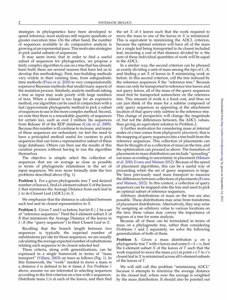
strategies in phylogenetics have been developed tospeed inference, most analyses still require quadratic orgreater execution time. On the other hand, the numberof sequences available to do comparative analysis isgrowing at an exponential pace. This motivates strategiesto pick useful subsets of sequences.

It may seem ironic that in order to find a usefulsubset of sequences for phylogenetics, we propose afairly complex algorithm to use on a tree that has alreadybeen built; there are several reasons that have led us todevelop this methodology. First, tree-building methodsvary widely in their running time, from subquadratictime methods (Price et al. 2010) to very computationallyexpensive Bayesian methods that model many aspects ofthe mutation process. Similarly, analytic methods takinga tree as input may scale poorly with large numbersof taxa. When a dataset is too large for an expensivemethod, our algorithm can be used in conjunction with afast/approximate phylogenetic method to pick a subsetof sequences to use in the more complex method. Second,we note that there is a remarkable quantity of sequencesfor certain loci, such as over 2 million 16s sequencesfrom Release 10 of the RDP database (Cole et al. 2009).Because this number will continue to increase, and manyof these sequences are redundant, we feel the need tohave a principled method useful for curators to picksequences that can form a representative subset of theselarge databases. Others can then use the results of thiscuration process without having to run the algorithmthemselves.

The objective is simple: select the collection ofsequences that are on average as close as possiblein terms of phylogenetic relatedness to the set ofinput sequences. We now more formally state the twoproblems described above (Fig. 1).

Problem 1. For a given phylogenetic tree T and desirednumber of leaves k, find a k-element subset X of the leavesL that minimizes the Average Distance from each leaf inL to its Closest Leaf (ADCL) in X.

We emphasize that the distance is calculated betweeneach leaf and its closest representative in X.

Problem 2. Given T and k as before, but let R⊂L be a setof “reference sequences.” Find the k-element subset X ofR that minimizes the Average Distance of the leaves inL\R (the “query sequences”) to their Closest Leaf in X.

Recalling that the branch length between twosequences is typically the expected number ofsubstitutions per site for those sequences, we are usuallycalculating the average expected number of substitutionsrelating each sequence to its closest selected leaf.

These criteria, along with generalizations, can beexpressed in a single framework in terms of “masstransport” (Villani, 2003) on trees as follows (Fig. 1). Inthis framework, the “work” needed to move a mass ma distance d is defined to be m times d. For Problem 1above, assume we are interested in selecting sequencesaccording to the first criterion on a tree with n sequences.Distribute mass 1/n at each of the leaves, and then find

the set X of k leaves such that the work required tomove the mass to one of the leaves in X is minimized.This is equivalent to minimizing the ADCL criterion,because the optimal solution will have all of the massfor a single leaf being transported to its closest includedleaf, incurring a cost of that distance divided by n; thesum of these individual quantities of work will be equalto the ADCL.

In a similar way, the second criterion can be phrasedas evenly dividing a unit of mass among the tips of L\R,and finding a set X of leaves in R minimizing work asbefore. In this second criterion, call the tree induced bythe reference sequences R the “reference tree.” Becausemass can only be transported to reference tree leaves andnot query leaves, all of the mass of the query sequencesmust first be transported somewhere on the referencetree. This amount of work is a fixed cost, and thus wecan just think of the mass for a subtree composed ofonly query sequences as appearing at the attachmentlocation of that query-only subtree to the reference tree.This change of perspective will change the magnitudeof, but not the differences between, the ADCL values,thus giving an equivalent solution to Problem 2.

A further motivation for considering mass at internalnodes of a tree comes from phylogenetic placement, that isthe mapping of query sequences into a tree built from thereference sequences. This collection of placements canthen be thought of as a collection of mass on the tree, andthe optimization can proceed as above. The transition ofplacements to mass distribution can include “spreading”out mass according to uncertainty in placement (Matsenet al. 2010; Evans and Matsen 2012). Because of the speedof placement algorithms, this can be a useful way ofproceeding when the set of query sequences is large.We have previously used mass transport to measurethe differences between collections of placements (Evansand Matsen, 2012). In this context, a collection of querysequences can be mapped onto the tree and used to pickan optimal subset of reference sequences.

Arbitrary distributions of mass on the tree are alsopossible. These distributions may arise from transformsof placement distributions. Alternatively, they may ariseby assigning an arbitrary value to various locations onthe tree; these values may convey the importance ofregions of a tree for some analysis.

Because all of these can be formulated in terms ofmass on a phylogenetic tree, rather than consideringProblems 1 and 2 separately, we solve the followinggeneralization of both of them.

Problem 3. Given a mass distribution � on aphylogenetic tree T with n leaves and some 0<k<n, findthe k-element subset X of the leaves of T such that thework required to move the mass �(x) at point x∈T to x’sclosest leaf in X is minimized across all k-element subsetsof the leaves of T.

We will still call this problem “minimizing ADCL”because it attempts to minimize the average distanceto the closest leaf, where now the average is weightedby the mass distribution. It should also be pointed out

by guest on September 14, 2013

http://sysbio.oxfordjournals.org/D

ownloaded from



2013 MATSEN ET AL.—MINIMIZING THE AVERAGE DISTANCE TO A CLOSEST LEAF 3

Problem 1

Problem 2

FIGURE 1. A diagram showing two example ADCL minimization problems. The k selected leaves are marked with hollow stars; in this casek =2. Problem 1 is to minimize the average distance from each leaf to its closest selected leaf. Problem 2 is to minimize the average distance fromthe query sequences (gray branches) to their closest reference sequence (reference sequence subtree in black). Both of these problems can bethought of as instances of Problem 3, which is to minimize the work required to move mass (gray circles) to a subset of k leaves. In Problem 1,a unit of mass is uniformly divided among the leaves of the tree. In Problem 2, mass is distributed in proportion to the number of query leavesthat attach at that point.

that the distances used in the ADCL framework are thedistances in the original tree. When leaves are pruned outof the tree, a tree built de novo on this reduced set willhave different branch lengths than the original tree withbranches pruned out; we do not attempt to correct forthat effect here. A more formal statement of Problem 3is made in the Appendix.

Problem 1 is equivalent to the DC1 criteriaindependently described in chapter 5 of BarbaraHolland’s Ph.D. thesis (Holland, 2001). She writes outthe criterion (among others), discusses why it mightbe biologically relevant, describes the computationalcomplexity of the brute-force algorithm, and does someexperiments comparing the brute-force to the greedyalgorithm.

We also note that the work described here shares somesimilarities with the Maximizing Minimum Distance(MMD) criterion of Bordewich et al. (2008). In thatcriterion, the idea is to select the subset X of leavessuch that the minimum distance between any two leavesin X is maximized across subsets of size k. The MMDcriterion has more similarities with PD maximizationthan it does with Problem 1. Moreover, the MMDanalog of Problem 2 (minimizing the maximum distanceof a reference sequence to a query sequence) wouldbe highly susceptible to off-target query sequences,such as sequences that are similar to but not actuallyhomologous to the reference set. Because of this

difference in objective functions, we have not attempteda comparison with MMD here.

The analogous problem in the generalnonphylogenetic setting is the classical k-medoidsproblem where k “centers” are found minimizing theaverage distance from each point to its closest center.The Partitioning Around Medoids (PAM) algorithm(described below) is a general heuristic for suchproblems, although our exact algorithm, which is basedon additivity of distances in a tree, will not work. Itappears that the complexity of exact k-medoids is notknown and is only bounded above by the obviousbrute-force bound. The simpler setting of k-means inthe plane has been shown to be NP-hard by Mahajanet al. (2009).

We emphasize that for the purposes of this article,we assume that k has been chosen ahead of time.Although we consider choosing an appropriate k to bean interesting direction for future work, as described inthe discussion, the choice will depend substantially onthe goals of the user.

METHODS

In this section, we will investigate methods tominimize ADCL for a given mass distribution as inProblem 3. We will first show that the greedy algorithm



ownloaded from




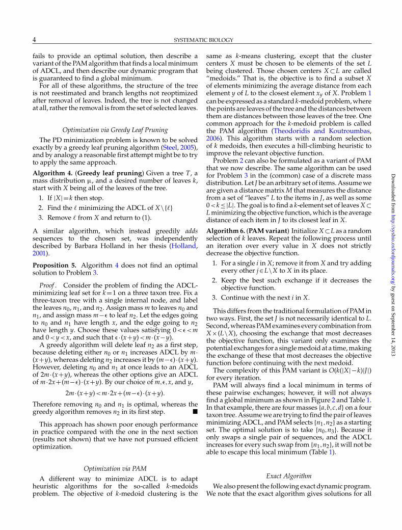
fails to provide an optimal solution, then describe avariant of the PAM algorithm that finds a local minimumof ADCL, and then describe our dynamic program thatis guaranteed to find a global minimum.

For all of these algorithms, the structure of the treeis not reestimated and branch lengths not reoptimizedafter removal of leaves. Indeed, the tree is not changedat all, rather the removal is from the set of selected leaves.

Optimization via Greedy Leaf PruningThe PD minimization problem is known to be solved

exactly by a greedy leaf pruning algorithm (Steel, 2005),and by analogy a reasonable first attempt might be to tryto apply the same approach.

Algorithm 4. (Greedy leaf pruning) Given a tree T, amass distribution �, and a desired number of leaves k,start with X being all of the leaves of the tree.

1. If |X|=k then stop.2. Find the � minimizing the ADCL of X\{�}3. Remove � from X and return to (1).

A similar algorithm, which instead greedily addssequences to the chosen set, was independentlydescribed by Barbara Holland in her thesis (Holland,2001).

Proposition 5. Algorithm 4 does not find an optimalsolution to Problem 3.

Proof . Consider the problem of finding the ADCL-minimizing leaf set for k =1 on a three taxon tree. Fix athree-taxon tree with a single internal node, and labelthe leaves n0, n1, and n2. Assign mass m to leaves n0 andn1, and assign mass m−� to leaf n2. Let the edges goingto n0 and n1 have length x, and the edge going to n2have length y. Choose these values satisfying 0<�<mand 0<y<x, and such that �·(x+y)<m·(x−y).

A greedy algorithm will delete leaf n2 as a first step,because deleting either n0 or n1 increases ADCL by m·(x+y), whereas deleting n2 increases it by (m−�)·(x+y).However, deleting n0 and n1 at once leads to an ADCLof 2m·(x+y), whereas the other options give an ADCLof m·2x+(m−�)·(x+y). By our choice of m,�,x, and y,

2m·(x+y)<m·2x+(m−�)·(x+y).

Therefore removing n0 and n1 is optimal, whereas thegreedy algorithm removes n2 in its first step. �

This approach has shown poor enough performancein practice compared with the one in the next section(results not shown) that we have not pursued efficientoptimization.

Optimization via PAMA different way to minimize ADCL is to adapt

heuristic algorithms for the so-called k-medoidsproblem. The objective of k-medoid clustering is the

same as k-means clustering, except that the clustercenters X must be chosen to be elements of the set Lbeing clustered. Those chosen centers X ⊂L are called“medoids.” That is, the objective is to find a subset Xof elements minimizing the average distance from eachelement y of L to the closest element xy of X. Problem 1can be expressed as a standard k-medoid problem, wherethe points are leaves of the tree and the distances betweenthem are distances between those leaves of the tree. Onecommon approach for the k-medoid problem is calledthe PAM algorithm (Theodoridis and Koutroumbas,2006). This algorithm starts with a random selectionof k medoids, then executes a hill-climbing heuristic toimprove the relevant objective function.

Problem 2 can also be formulated as a variant of PAMthat we now describe. The same algorithm can be usedfor Problem 3 in the (common) case of a discrete massdistribution. Let J be an arbitrary set of items. Assume weare given a distance matrix M that measures the distancefrom a set of “leaves” L to the items in J, as well as some0<k ≤|L|. The goal is to find a k-element set of leaves X ⊂L minimizing the objective function, which is the averagedistance of each item in J to its closest leaf in X.

Algorithm 6. (PAM variant) Initialize X ⊂L as a randomselection of k leaves. Repeat the following process untilan iteration over every value in X does not strictlydecrease the objective function.

1. For a single i in X; remove it from X and try addingevery other j∈L\X to X in its place.

2. Keep the best such exchange if it decreases theobjective function.

3. Continue with the next i in X.

This differs from the traditional formulation of PAM intwo ways. First, the set J is not necessarily identical to L.Second, whereas PAM examines every combination fromX×(L\X), choosing the exchange that most decreasesthe objective function, this variant only examines thepotential exchanges for a single medoid at a time, makingthe exchange of these that most decreases the objectivefunction before continuing with the next medoid.

The complexity of this PAM variant is O(k(|X|−k)|J|)for every iteration.

PAM will always find a local minimum in terms ofthese pairwise exchanges; however, it will not alwaysfind a global minimum as shown in Figure 2 and Table 1.In that example, there are four masses {a,b,c,d} on a fourtaxon tree. Assume we are trying to find the pair of leavesminimizing ADCL, and PAM selects {n1,n2} as a startingset. The optimal solution is to take {n0,n3}. Because itonly swaps a single pair of sequences, and the ADCLincreases for every such swap from {n1,n2}, it will not beable to escape this local minimum (Table 1).

Exact AlgorithmWe also present the following exact dynamic program.

We note that the exact algorithm gives solutions for all



ownloaded from




a

b c

d6

0.3322n

3n

1n0n

1

6

2

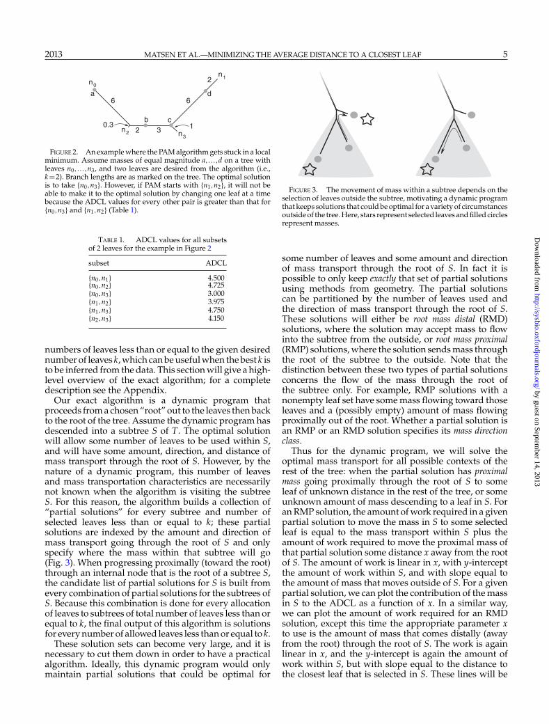
FIGURE 2. An example where the PAM algorithm gets stuck in a localminimum. Assume masses of equal magnitude a,...,d on a tree withleaves n0,...,n3, and two leaves are desired from the algorithm (i.e.,k =2). Branch lengths are as marked on the tree. The optimal solutionis to take {n0,n3}. However, if PAM starts with {n1,n2}, it will not beable to make it to the optimal solution by changing one leaf at a timebecause the ADCL values for every other pair is greater than that for{n0,n3} and {n1,n2} (Table 1).

TABLE 1. ADCL values for all subsetsof 2 leaves for the example in Figure 2

subset ADCL

{n0,n1} 4.500{n0,n2} 4.725{n0,n3} 3.000{n1,n2} 3.975{n1,n3} 4.750{n2,n3} 4.150

numbers of leaves less than or equal to the given desirednumber of leaves k, which can be useful when the best k isto be inferred from the data. This section will give a high-level overview of the exact algorithm; for a completedescription see the Appendix.

Our exact algorithm is a dynamic program thatproceeds from a chosen “root” out to the leaves then backto the root of the tree. Assume the dynamic program hasdescended into a subtree S of T. The optimal solutionwill allow some number of leaves to be used within S,and will have some amount, direction, and distance ofmass transport through the root of S. However, by thenature of a dynamic program, this number of leavesand mass transportation characteristics are necessarilynot known when the algorithm is visiting the subtreeS. For this reason, the algorithm builds a collection of“partial solutions” for every subtree and number ofselected leaves less than or equal to k; these partialsolutions are indexed by the amount and direction ofmass transport going through the root of S and onlyspecify where the mass within that subtree will go(Fig. 3). When progressing proximally (toward the root)through an internal node that is the root of a subtree S,the candidate list of partial solutions for S is built fromevery combination of partial solutions for the subtrees ofS. Because this combination is done for every allocationof leaves to subtrees of total number of leaves less than orequal to k, the final output of this algorithm is solutionsfor every number of allowed leaves less than or equal to k.

These solution sets can become very large, and it isnecessary to cut them down in order to have a practicalalgorithm. Ideally, this dynamic program would onlymaintain partial solutions that could be optimal for

FIGURE 3. The movement of mass within a subtree depends on theselection of leaves outside the subtree, motivating a dynamic programthat keeps solutions that could be optimal for a variety of circumstancesoutside of the tree. Here, stars represent selected leaves and filled circlesrepresent masses.

some number of leaves and some amount and directionof mass transport through the root of S. In fact it ispossible to only keep exactly that set of partial solutionsusing methods from geometry. The partial solutionscan be partitioned by the number of leaves used andthe direction of mass transport through the root of S.These solutions will either be root mass distal (RMD)solutions, where the solution may accept mass to flowinto the subtree from the outside, or root mass proximal(RMP) solutions, where the solution sends mass throughthe root of the subtree to the outside. Note that thedistinction between these two types of partial solutionsconcerns the flow of the mass through the root ofthe subtree only. For example, RMP solutions with anonempty leaf set have some mass flowing toward thoseleaves and a (possibly empty) amount of mass flowingproximally out of the root. Whether a partial solution isan RMP or an RMD solution specifies its mass directionclass.

Thus for the dynamic program, we will solve theoptimal mass transport for all possible contexts of therest of the tree: when the partial solution has proximalmass going proximally through the root of S to someleaf of unknown distance in the rest of the tree, or someunknown amount of mass descending to a leaf in S. Foran RMP solution, the amount of work required in a givenpartial solution to move the mass in S to some selectedleaf is equal to the mass transport within S plus theamount of work required to move the proximal mass ofthat partial solution some distance x away from the rootof S. The amount of work is linear in x, with y-interceptthe amount of work within S, and with slope equal tothe amount of mass that moves outside of S. For a givenpartial solution, we can plot the contribution of the massin S to the ADCL as a function of x. In a similar way,we can plot the amount of work required for an RMDsolution, except this time the appropriate parameter xto use is the amount of mass that comes distally (awayfrom the root) through the root of S. The work is againlinear in x, and the y-intercept is again the amount ofwork within S, but with slope equal to the distance tothe closest leaf that is selected in S. These lines will be



ownloaded from




subwork parameter

wor

k

FIGURE 4. A visual depiction of the method of removing partialsolutions that could not be optimal for any setting in the rest of thetree. Each line represents the total work for a partial solution that hassubwork parameter x. Because the dashed lines are not minimal forany value of x, they can be discarded.

called subwork lines, and the parameter x will be calledthe subwork parameter.

The only partial solutions that could form part ofan optimal solution are those that are optimal forsome value of the subwork parameter (Fig. 4). Thisoptimization can be done using well-known algorithmsin geometry. Imagine that instead of considering theminimum of a collection of subwork lines, we areusing these lines to describe a subset of the planeusing inequalities. Some of these inequalities arespurious and can be thrown away without changing thesubset of the plane; the rest are called facets (Ziegler,1995). Our implementation uses Komei Fukuda’scddlib implementation (Fukuda, 2012) of the doubledescription method (Fukuda and Prodon, 1996) to findfacets. The complexity of our exact algorithm is difficultto assess, given that in the words of Fukuda andProdon (1996), “we can hardly state any interestingtheorems on [the double description algorithm’s] timeand space complexities.” We note that our code uses thefloating point, rather than exact arithmetic, version ofcddlib because branch lengths are typically obtained bynumerical optimization to a certain precision. For thisreason, our implementation is susceptible to roundingerrors, and ADCLs are only compared to within a certainprecision in the implementation.

RESULTS

We have developed and implemented algorithms tominimize the ADCL among subsets of leaves of thereference tree. These algorithms are implemented as themin_adcl_tree (Problem 1) and min_adcl (Problems 1, 3)subcommands of the rppr binary that is part ofthe pplacer (http://matsen.fhcrc.org/pplacer/) suite ofprograms. The code for all of the pplacer suite is freelyavailable (http://github.com/matsen/pplacer).

Our PAM implementation follows Algorithm 6. Wefound this variant, which makes the best exchange

at each medoid rather than the best exchange overall medoids, to converge two orders of magnitudemore rapidly than a traditional PAM implementation(Supplementary Figs. S3 and S4).

We used simulation to understand the frequency withwhich PAM local minima are not global minima as inFigure 2, as well as the relative speed of PAM and theexact algorithm. For tree simulation, random trees weregenerated according to the Yule process (Yule, 1925);branch lengths were drawn from the � distribution withshape parameter 2 and scale parameter 1. We evaluatedthree datasets: two “tree” sets and one “mass” set. Forthe “tree” test sets, trees were randomly generated asdescribed, resulting in 5 trees of 1000 leaves each, and acollection of trees with 10 to 2500 leaves in incrementsof 10 leaves. Problem 1 was then solved using eachalgorithm for each “tree” test set; for the 1000 leaf trees kwas set to each number from 1 to 991 congruent to 1 mod10, and for the large collection of trees k was set to half thenumber of leaves. For the “mass” test set, one tree wasbuilt for each number of leaves from 5 to 55 (inclusive);for each of these trees, m masses were assigned touniformly selected edges of the tree at uniform positionson the edges, where m ranged from 5 to 95 massesin 10-mass increments. All of these simulated test setshave been deposited in Dryad (http://datadryad.org/handle/10255/dryad.41611). Problem 2 was then solvedusing each algorithm with k equal to (the ceiling of) halfthe number of leaves.

The PAM heuristic typically works well. Although wehave shown above that the PAM algorithm does getstuck in local minima (Fig. 2), it did so rarely on the“mass” dataset (Fig. 5); similar results were obtainedfor the “tree” dataset (results not shown). As might beexpected, PAM displays the greatest speed advantagein when k is rather large on the “tree” dataset (Fig. 6).PAM is slowest for k equal to n/2 because that valueof k has the largest number of possible k-subsets; oncek>n/2 it gets faster because there are fewer choices asfar as what to select. PAM is faster for small trees thanthe exact algorithm on the “tree” dataset (Fig. 7), anduses less memory (Supplementary Fig. S2). We note inpassing that the ADCL improvement from PAM is notmonotonically nonincreasing, which is to say that it ispossible to have a small improvement followed by a largeimprovement.

The currently available tools for automatic selectionof reference sequences include the use of an algorithmthat maximizes PD or using a random set of sequences(Redd et al. 2011). Others have pointed out that longpendant branch lengths are preferentially chosen by PDmaximization, even when additional “real” diversity isavailable (Bordewich et al. 2008). Long pendant branchlengths can be indicative of problematic sequences, suchas chimeras or sequencing error.

We designed an experiment to measure the extentto which the ADCL algorithm would pick problematicsequences compared with PD maximization and randomselection. We downloaded sequences with taxonomicannotations from GenBank belonging to the family



ownloaded from




FIGURE 5. Comparison between the ADCL results obtained bythe exact algorithm and the PAM heuristic on the “mass” test set. Thepoints are black triangles when the difference in ADCL between PAMand the exact algorithm is greater than 10−5.

FIGURE 6. Comparison of the time required to run the exact algorithmversus PAM with respect to the number of leaves selected to keep. Fivetrees were generated of 1000 leaves each, and for each number k from1 to 991 congruent to 1 mod 10, both algorithms were run to keep k ofthe leaves. The mean and standard errors are shown here.

Enterobacteriaceae, and identified chimeric sequencesusing UCHIME (Edgar et al. 2011). We built a tree ofconsisting of these sequences and other sequences fromthe same species from the RDP database release 10,update 28 (Cole et al. 2009). Five sequences were chosenfor each species (when such a set existed). RemainingRDP sequences from these species were then placedon this tree using pplacer (Matsen et al. 2010) andthe full algorithm was used to pick some fraction xof the reference sequences. In this case, using the fullalgorithm to minimize ADCL was less likely to choosechimeric sequences than choosing at random, whereasPD maximization was more likely to choose chimericsequences (Fig. 8). The ADCL for the full algorithm wassubstantially lower than for either PD maximization or

FIGURE 7. Comparison of the time required to run the exact algorithmversus PAM with respect to the number of leaves in the original tree.Trees were generated with 10 to 2500 leaves in increments of 10 leaves;each tree was pruned to half of the original number of leaves. The resultof running each algorithm on a given tree is shown here as a single linewith x-position equal to the number of leaves of that tree, whereas thetwo y-positions of the line show the times taken by the two algorithms;when the exact algorithm was faster the line is black and when PAMwas faster the line is gray. A point on each line shows the time for thePAM algorithm.

random subset selection, as would be expected given thatADCL is explicitly minimized in our algorithms.

We are not proposing this algorithm as a new wayto find sequences of poor quality, rather, it is a way ofpicking sequences that are representative of the localdiversity in the tree. The chimera work above was tomake the point that artifactual sequences clearly notrepresentative of actual diversity do not get chosen,while they do using the PD criterion. We also notethat because bootstrap resampling can change branchlength and tree topology, the minimum ADCL set is notguaranteed to be stable under bootstrapping. However,in the cases we have evaluated, the minimum ADCLvalue itself is relatively stable to bootstrap resamplingwhen k is not too small (Supplementary Fig. S1,doi:10.5061/dryad.md023/6).

DISCUSSION

In this article, we described a simple new criterion,minimizing the ADCL, for finding a subset of sequencesthat either represent the diversity of the sequences ina sample or are close on average to a set of querysequences. In doing so, abundance information is takeninto account in an attempt to strike a balance betweenoptimality and centrality in the tree. In particular, thiscriterion is the only way of which we are aware to picksequences that are phylogenetically close on averageto a set of query sequences. We have also investigatedmeans of minimizing the ADCL, including a heuristicthat performs well in practice and an exact dynamicprogram. ADCL minimization appears to avoid pickingchimeric sequences.



ownloaded from




FIGURE 8. ADCL values and proportion of chimeric sequences kept for random selection, PD maximization, and ADCL minimization runon a set of Enterobacteriaceae 16s sequences along with chimeras from the same family identified with UCHIME (Edgar et al. 2011).

The current implementations are useful for moderate-size trees; improved algorithms will be needed for large-scale use (Fig. 7). We have found present algorithmsto be quite useful in a pipeline that clusters querysequences by pairwise distance first, then retrieves acollection of potential reference sequences per clusteredgroup of query sequences, then uses the ADCL criterionfor selecting potential reference sequences among those(manuscript under preparation). This has the advantageof keeping the number of input sequences within amanageable range, as well as ensuring that the numberof reference sequences is comprehensive across the tree.

The computational complexity class of the ADCLoptimization problem is not yet clear.

Because of the special geometric structure of theproblem, there is almost certainly room for improvementin the algorithms used to optimize ADCL. Only asubset of the possible exchanges need to be tried ineach step of the PAM algorithm, and more intelligentmeans could be used for deciding which mass needsto be reassigned, similar to the methods of Zhang andCouloigner (2005). A better understanding of situationssuch as those illustrated by Figure 4 could lead toan understanding of when PAM becomes stuck inlocal optima. The geometric structure of the optimalityintervals could be better leveraged for a more efficientexact algorithm. The PAM algorithm may also reacha near-optimal solution quickly, then use substantialtime making minimal improvements to converge tothe minimum ADCL (Supplementary Fig. S3). If anapproximate solution is acceptable, alternate stoppingcriteria could be used.

In future work, we also plan on investigating thequestion of what k is appropriate to use for a givenphylogenetic tree given certain desirable characteristicsof the cut-down set. We note that using the exact

algorithm makes it easy to find a k that corresponds to anupper bound for ADCL, but the choice of an appropriateupper bound depends on the application and prioritiesof the user. For example, in taxonomic assignment, somemay require subspecies-level precision, whereas othersrequire assignments only at the genus or higher level;the needs for ADCL would be different in these differentcases.

SUPPLEMENTARY MATERIAL

Supplementary material, including data files andfigures, can be found in the Dryad data repository athttp://datadryad.org, doi:10.5061/dryad.md023/6.

FUNDING

The authors are supported by NIH [grant R01HG005966-01, NIH grant R37-AI038518], and by startupfunds from the Fred Hutchinson Cancer ResearchCenter.

ACKNOWLEDGMENTS

F.A.M. thanks Christian von Mering for remindinghim that phylogenetic diversity often picks sequencesof low quality, and Steve Evans for helping think aboutthe formulation of mass on trees, as well as pointingout the “medoids” literature. All authors are gratefulto Sujatha Srinivasan, Martin Morgan, David Fredricks,and especially Noah Hoffman for helpful comments.Aaron Darling, Mark Holder, Barbara Holland, and twoanonymous reviewers provided feedback that greatlyimproved the form and content of the article.



ownloaded from




APPENDIX: A MORE COMPLETE DESCRIPTION OF ADCLMINIMIZATION

The distance d(·,·) between points on a tree is definedto be the length of the shortest path between those points.A rooted subtree is a subtree that can be obtained froma rooted tree T by removing an edge of T and takingthe component that does not contain the original root ofT. The proximal direction in a rooted tree means towardthe root, whereas the distal direction means away fromthe root. We emphasize that the phylogenetic trees hereare considered as collections of points with distancesbetween them, that is metric spaces, such that by a subsetof a phylogenetic tree we mean a subset of those points.

Introduction to ADCLDefinition 1 A mass map on a tree T is a Borel measureon T. A mass distribution on a tree T is a Borel probabilitymeasure on T.

Definition 2 Given a subset X ⊂L(T) of leaves and amass distribution �, define the ADCL to be the expecteddistance of a random point distributed according to � toits closest leaf in X. That is,

ADCL�(X)=E

[min�∈X

d(P,�)],

where P∼�.

Problem 7. Minimize ADCL for a given numberof allowed leaves. That is, given 0<k ≤|L(T)| andprobability measure �, find the X ⊂L(T) with |X|=kminimizing ADCL�(X).

The expected distance of a randomly sampled pointP∼� to a fixed point � is equal to the amount of workrequired to move mass distributed according � to thepoint �, when work is defined as mass times distance.

Voronoi RegionsIn this section, we connect the above description with

the geometric concept of a Voronoi diagram.

Definition 3 Given a subset X ⊂L(T) of leaves and �∈X,the Voronoi region V(�,X) for leaf � is the set of points ofT such that the distance to � is less than or equal to thedistance to any other leaf in X. The Voronoi diagram for aleaf set X in the tree is the collection of Voronoi regionsfor the leaves in X.

Note that the Voronoi regions by this definition areclosed sets that are not disjoint; they intersect each otherin discrete points where the distances to leaves are equal.

Definition 4 Given a subset Z of T, a mass distribution� and a leaf �, let ��(Z,�) be the work needed to movethe mass of � in Z to the leaf �.

The following simple lemma allows us to express theADCL in terms of the Voronoi regions.

Lemma 8. Let � be a mass distribution. Then

ADCL�(X)=∑�∈X

��(V(�,X),�). (1)

Proof . For a given p∈T,

min�∈X

d(p,�)=∑�∈X

1V(�,X)(p)d(p,�),

where 1V(�,X) is the indicator function for the set V(�,X).Let P∼�. Then

E

[min�∈X

d(P,�)]=∫

p∈Tmin�∈X

d(p,�)d�

=∑�∈X

∫p∈V(�,X)

d(p,�)d�

=∑�∈X

��(V(�,X),�)

where the last step is by the optimization definition ofthe KR distance (Evans and Matsen, 2012). �

Dynamic ProgramBackground.—This section presents a full solution toProblem 7 via a dynamic program. This dynamicprogram will descend through the tree selecting eachrooted subtree S in a depth-first manner, and solvingthe optimization for every amount and direction of masstransport through the root of S. Because the algorithmconstructs every solution that is not suboptimal, thealgorithm is exact.

Bubbles.—A first observation for the exact algorithm isthat the tree can be divided into connected sets, that wecall bubbles, with the following property: irrespective ofthe set of leaves X of the tree T that are selected, anypair of points in the same bubble will share the sameclosest leaf in X. Because of this characteristic, all thatis needed to decide the fate of every particle of mass isto decide optimal mass transport on a per-bubble basis.Indeed, if it is optimal to move mass at point p to a leaf�, then the same must be true for every other point q inin the bubble. This observation turns the search for anoptimal subset into an optimal assignment of bubbles toleaves of the tree, such that the total number of leavesthat are assigned a bubble has cardinality at most k. Asdescribed below, the partition of the tree into bubbles isin fact the refinement of all possible Voronoi diagramsfor all subsets of the leaves (along with the partition byedges, which is put in for convenience).

Recall that partitions of a set are partially orderedby inclusion, such that A≤A′ for two partitions A andA′ iff every V ∈A is contained in a V′ ∈A′. Partitionsare a complete lattice with this partial order, thus thereexists a greatest lower bound for any collection ofpartitions; define A∧B be the greatest lower bound for



ownloaded from




any partitions A and B. In practice, this means findingthe “coarsest” partition such that pairwise intersectionsof sets in the partitions are represented: for example,

{A,X\A}∧{B,X\B}={A∩B,A\B,B\A,X\(A∪B)}.We will be interested in partitions of phylogenetic trees,and the boundaries of partitions can be thought of as“cuts” on edges or internal nodes. Thus if A and B aretwo partitions of a tree T, A∧B is the partition with every“cut.”

Let V(X) be the Voronoi diagram of T for some subsetX of the leaves of T. Let E be the partition of T such thatthe edges of T are the sets of the partition.

Definition 5 The bubble partition of a tree T is the coarsestpartition refining all of the Voronoi decompositions of Tand the edge partition:

B(T) :=E ∧∧

X⊂L(T)

V(X).

This partition forms the basis of our approach. ByLemma 8, an exhaustive approach to Problem 7 wouldinvolve trying all Voronoi diagrams for a given tree andtransporting the mass in each of the regions to the closestleaf. However, B(T) is the refinement of all Voronoipartitions. Because every point in a bubble has the sameclosest leaf, every optimal solution can be completelydescribed by deciding to what leaf the mass in B gets sentfor each B∈B(T). The number of bubbles is quadraticin the number of leaves irrespective of the given massdistribution.

In particular, by describing the optimization algorithmin terms of bubbles, it will work in the case of acontinuous mass distribution. What is needed is a wayto calculate the amount of work needed to move acontinuous mass distribution to one side of a bubble.This can be done using a simple integral as described in(Evans and Matsen, 2012), however, the above-describedrppr implementation is in terms of a discrete distributionof mass.

Recursion introduction.—In this section, we will describea recursion that will solve Problem 7 as described above.Fix the number of allowed leaves k. The recursion isdepth-first starting at a root, which can be arbitrarilyassigned if the tree is not already rooted. Partial solutionsstart at the leaves, are modified and reproduce as theytravel through bubbles, then get combined at internalnodes. We remind the reader that a solution to Problem 7is completely specified by the destination of the mass foreach bubble.

These partial solutions will be denoted by labeledtuples, either RMD(X,�,ω) for a root mass distal solutionor RMP(X,�,,ω) for a root mass proximal solutionas follows. The X component of the partial solution isthe leaf set: the leaves that have been selected for thepartial solution to the ADCL problem. The� componentis the closest leaf distance: the distance to the closestleaf in the partial solution. The component is the

proximal mass: the mass that is moved to the root of S bythis partial solution (RMD solutions always have zeroproximal mass). The ω component is the work subtotal:the amount of work needed for the partial solution tomove the mass in S to either the root of S or a leaf in X.Whether a partial solution is an RMP or an RMD solutiondefines its mass direction class.

The depth-first recursion will maintain a list of partialsolutions that gets updated upon traversing bubbles andinternal nodes. We remind the reader that bubbles neverspan more than a single edge.

Base case at a leaf.—There are two base cases at a leaf:that of not including the leaf and that of including theleaf. The partial solution that corresponds to includingthe leaf � is RMD({�},0,0) and that of not including theleaf is RMP(∅,∞,0,0). From there, we move proximallythrough the bubbles along the edges and throughthe internal nodes as follows. Note that these partialsolutions at each leaf are then passed through thebubbles directly proximal to their leaf.

Moving through a bubble.—Assume the algorithm istraversing a bubble along an edge, such that the edgelength in the bubble is and the amount of mass in thebubble is �. Define � to be the amount of work requiredto move the mass in the bubble to the distal side of thebubble, and � to be the corresponding amount of workfor the proximal side. We now describe the steps requiredto update this collection of partial solutions going fromthe distal to the proximal side of the bubble.

The first step is to update the existing partial solutions.In this updating step, the mass-direction class willnot be changed (in the second step we will constructRMP solutions from RMD solutions). RMD solutions getupdated as follows:

RMD(X,�,ω)

maps toRMD(X,�+,ω+�+�·�)

as RMD solutions must move the mass of the currentbubble to a leaf, and moving it to the closest selected leafis optimal.

On the other hand, RMP solutions will have the massof the current bubble moving away from the leaves of S.Thus

RMP(X,�,,ω)maps to

RMP(X,�+,+�,ω+�+·).

The second step is to consider solutions such thatthe mass transport on the distal and proximal sides ofthe bubble are not the same. In that case, the optimaldirections of mass movement on distal and proximaledges for a given bubble must be pointing away fromeach other; the alternative could not be optimal. Thushere we consider adding an RMP solution based on aprevious RMD solution. This solution has all of the mass



ownloaded from




going to the leaves in S except that of the current bubble,which moves proximally. This step can be ignored if�=0. Given a RMD(X,�,ω) with X =∅, add the resulting

RMP(X,�+,�,ω+�)

to the list of possible solutions if �<�+�·�.The following simple lemma reduces the number of

bubbles that must be considered.

Lemma 9. Given two neighboring bubbles on a singleedge, such that the proximal bubble has zero mass. Therecursive step in this section after progressing throughthese two bubbles is identical to one where the twobubbles are merged. �

Moving proximally through an internal node.—Whenencountering an internal node, the algorithm firstcombines all tuples of partial solutions for each subtreeas follows. Assume we are given one ϕi from each of thesubtrees, where Xi, �i,i, andωi are as above for the i-thtree (define i =0 for RMD solutions).

At least one, and possibly two, partial solutions canbe constructed from the partial solutions in the subtrees.There is always one solution where the proximal mass,if it exists, continues moving away from the leaves of S;we will call this the “continuing” solution. Sometimes itis also possible for the proximal mass to go to a leaf inone of the subtrees, giving another solution we will callthe “absorbing” solution.

The continuing solution in the case that all solutionsare RMD solutions is

RMD

(⋃i

Xi,mini�i,∑

i

ωi

).

If any of the solutions are RMP solutions, then theresulting solution is

RMP

(⋃i

Xi,mini�i,∑

i

i,∑

i

ωi

)

where i =0 for RMD solutions.Now, if at least one leaf is selected in one of the

subtrees, then it could be optimal to move the proximalmass to the closest leaf of the existing RMD solutions tomake an absorbing solution; in that case we also havethe new RMD solution

RMD

(⋃i

Xi,mini�i,∑

i

ωi +(

mini�i

)·∑

i

i

).

Given an internal node with k subtrees, combine allpartial solutions of the subtrees in this way. The completecollection of solutions given a set of �i for each subtreeis the union of this process applied to every element ofthe Cartesian product of the �i. Throw away any partialsolutions such that the cardinality of the X is greaterthan k.

Termination at the root.—Select the RMP solutionRMP(X,�,ω) with |X|=k with the smallest ω. Note thatin fact all solutions for number of chosen leaves less thank are generated by this algorithm.

Avoiding computation of suboptimal solutions.—By naïvelycombining all of the solutions described above we mayget solutions that cannot be optimal for any structure ofthe rest of the tree. These solutions greatly reduce thespeed of the algorithm when carried along as describedabove. In this section, we describe a way to avoid thesesolutions using geometry (Fig. 4).

The culling strategy employed here is to eliminatepartial solutions that would not be optimal for anyamount and direction of mass transport through theroot of S. This is achieved by first binning the partialsolutions by the number of leaves k they employ thenfurther binning them by mass-direction class.

For an RMP solution, the amount of work requiredin a given partial solution to move the mass in S tosome selected leaf is equal to the mass transport within Splus the amount of work required to move the proximalmass of that partial solution to some leaf proximal to S.Imagine that this proximal leaf is distance x away fromthe root of S. For a given partial solution, we can plot theamount of work to move the mass in S to some selectedleaf with respect to x. This will be ω+x ·.

Similar logic applies for RMD solutions but where theappropriate parameter x to use is the amount of massthat comes proximally through �. The total amount ofwork in that case then, is ω+x ·�.

These considerations motivate the followingdefinition.

Definition 6 The subwork fϕ for a partial solution ϕ is thefunction

fϕ(x)={ω+x · if ϕ=RMP(X,�,,ω)ω+x ·� if ϕ=RMD(X,�,ω)

Let the x in fϕ(x) be called the subwork parameter.

Definition 7 Assume � is a set of partial solutionswith the same number of leaves and the same root massdirection. The optimality interval I�(ϕ) is the interval forwhich ϕ is optimal compared with the other solutions in�, namely

I�(ϕ)={x∈[0,∞) : fϕ(x)≤ fϕ′ (x)∀ϕ′ ∈�}.It can be easily seen that the set defined in this way is

actually an interval. We can ignore partial solutions thathave an empty optimality interval.

These optimality intervals can be found by usingthe double description algorithm as described inthe algorithm introduction. Specifically, a line withequation y=mx+b will get translated into the half-plane constraint y≤mx+b. The set of points in the planethat satisfy this collection of inequalities is called aconvex polytope. A convex polytope can be equivalentlydescribed as the intersection of a number of half-spaces(a so-called H-description) or as the convex hull of a



ownloaded from




number of points (a so-called V-description). In thissetting, the set of x values between vertices are theoptimality intervals, and the lines that contact pairs ofneighboring vertices correspond to partial solutions thatare optimal for some value of x (Fig. 4).

The “double description” algorithm (Motzkin et al.1983; Fukuda and Prodon 1996) is an efficient wayto go from an H-description to a V-description whichalso collects information on what linear constraintscontact what facets. One way to use this perspectiveon optimal solutions is to simply throw away partialsolutions that have empty optimality intervals aftercombining. Another is to use optimality intervals toguide the combination of solutions in at internal nodesas described in the next section.

We perform a prefiltering step before running thedouble description algorithm to discard lines that couldnever be facets. Denote lines as being pairs of (m,b),where m is a slope and b is a y-intercept. Clearly if m1<m2and b1<b2 then the line (m1,b1) will lie below (m2,b2)for all positive x. Therefore (m2,b2) will never be a facetand can be ignored. We quickly eliminate some of theseclearly suboptimal partial solutions by sorting the (m,b)pairs in terms of increasing m. If in this ordering, the line(m1,b1) precedes (m2,b2) with b2 ≥b1 then we discard(m2,b2).

We can also include some global information asinequalities. For RMP solutions, the subwork parameteris bounded between the closest and farthest leavesin the proximal part of the tree. For RMD solutions,the subwork parameter is bounded between zeroand the total amount of mass in the proximal partof the tree. These additional constraints further cutdown optimality intervals and reduce the number ofsolutions.

Optimality intervals and solution combination.—Here weexplore ways of using optimality intervals to reducethe number of partial solutions that must be combinedbetween subtrees. We will describe the partial solutionscombination in terms of combining pairs of subtrees. Ifa given internal node has more than two subtrees, sayT1,...,Tk , then we can combine over partial solutionsfor T1 and T2, then combine those results with T3, andso on.

Assume we are given two partial solutions ϕ1 andϕ2, and these have two optimality intervals I1 = (l1,u1)and I2 = (l2,u2), respectively. The criteria used to checkif a given combination could be optimal depend on themass-direction class, and we will describe the criteriaon a case-by-case basis. Let ϕ be the solution that isformed from the combination of ϕ1 and ϕ2, and denoteits optimality interval with I.

If ϕ1 and ϕ2 are both RMP solutions, the subworkparameter for each will be the distance to the closest leafin the proximal part of the tree. Since the combinationwill also be an RMP solution, to be optimal for a subworkparameter x each partial solution will have to be optimalfor that x. Thus I = I1 ∩I2, and ϕ is viable if I =∅.

If ϕ1 and ϕ2 are both RMD solutions, the subworkparameter is the amount of mass that comes proximallythrough the root of S. When mass comes proximallythrough the root, it will go to the subtree that has theclosest leaf. For this reason, I will be the optimalityinterval of the partial solution with the smallest �. If thesubtrees have identical �’s, then I is the smallest intervalcontaining I1 and I2.

Recall that when one partial solution is an RMPsolution and the other is an RMD solution, then we canget either an RMP or an RMD solution. Assume firstϕ1 isan RMP solution,ϕ2 is an RMD solution, andϕ is an RMPsolution. Sinceϕ is an RMP solution, no mass will be sentinto T2 from outside of it. Thus, ϕ should only be usedif ϕ2 has the smallest ω across all partial solutions thathave the same number of leaves as ϕ2. Also, the solutioncould be optimal only if �2 is greater than the upperbound of I1, because otherwise it would be optimal tosend the proximal mass of T1 proximally into T2. If ϕ1 isan RMP solution,ϕ2 is an RMD solution, andϕ is an RMDsolution, the subwork parameter for ϕ is the amount ofmass coming from above. Because the proximal massof ϕ1 will be sent into T2, the optimality interval I isI2 ∩[1,∞). The corresponding partial solution is validif I is nonempty and �2 ∈ I1.

REFERENCES

Berger S.A., Krompass D., Stamatakis A. 2011. Performance, accuracy,and web server for evolutionary placement of short sequence readsunder maximum likelihood. Syst. Biol. 60:291–302.

Bordewich M., Rodrigo A.G., Semple C. 2008. Selecting taxa to saveor sequence: desirable criteria and a greedy solution. Syst. Biol.57:825–834.

Cole J.R., Wang Q., Cardenas E., Fish J., Chai B., Farris R.J., Kulam-Syed-Mohideen A.S., McGarrell D.M., Marsh T., Garrity G.M. et al. 2009.The Ribosomal Database Project: improved alignments and newtools for rRNA analysis. Nucleic Acids Res. 37(suppl 1):D141–D145.

Edgar R.C., Haas B.J., Clemente J.C., Quince C., Knight R. 2011.Uchime improves sensitivity and speed of chimera detection.Bioinformatics, 27:2194–2200.

Eisen J.A., Sweder K.S., Hanawalt P.C. 1995. Evolution of theSNF2 family of proteins: subfamilies with distinct sequences andfunctions. Nucleic Acids Res. 23:2715–2723.

Eisen J.A. 1998. Phylogenomics: improving functional predictionsfor uncharacterized genes by evolutionary analysis. Genome Res.8:163–167.

Engelhardt B.E., Jordan M.I., Muratore K.E., Brenner S.E. 2005. Proteinmolecular function prediction by Bayesian phylogenomics. PLOSComp. Biol. 1:e45.

Evans S.N., Matsen F.A. 2012. The phylogenetic Kantorovich-Rubinstein metric for environmental sequence samples. J. Royal Stat.Soc. (B). 74:569–592.

Faith D.P. 1992. Conservation evaluation and phylogenetic diversity.Biol. Conserv. 61:1–10.

Fukuda K., Prodon A. 1996. Double description method revisited. InDeza, M., Euler, R., Manoussakis, I., editors. Combinatorics andComputer Science, Vol. 1120. 91–111.

Fukuda, K. 2012. cddlib library. Available from: http://www.cs.mcgill.ca/∼fukuda/soft/cdd_home/cdd.html, version 094f.

Holland B. 2001. Evolutionary analyses of large datasets: treesand beyond. [PhD thesis], Massey University. Available fromhttp://hdl.handle.net/10179/2078.

Mahajan M., Nimbhorkar P. Varadarajan, K. 2009. The planar k-meansproblem is NP-hard. In WALCOM: Algorithms and Computation.Chicago: Springer. 274–285.



ownloaded from




Matsen, F.A., Kodner, R.B., Armbrust, E.V. 2010. pplacer: lineartime maximum-likelihood and Bayesian phylogenetic placement ofsequences onto a fixed reference tree. BMC bioinfo. 11:538.

Minh B.Q., Klaere S., Von Haeseler A. 2006. Phylogenetic diversitywithin seconds. Syst. Biol. 55:769–773.

Motzkin T.S. Ralffa H., Thompson G.L., Thrall R.M. 1983. The doubledescription method. In: Cantor, D., Gordon, B., Rothschild, B.,Boston, B., editors. p. 81.

Pardi F. and Goldman N. 2005. Species choice for comparativegenomics: Being greedy works. PLOS Genet. 1:e71.

Piantadosi A., Chohan B., Chohan V., McClelland R.S., Overbaugh,J. 2007. Chronic HIV-1 infection frequently fails to protect againstsuperinfection. PLOS Pathogens, 3:e177.

Price M.N., Dehal P.S., Arkin, A.P. 2010. Fasttree 2–approximatelymaximum-likelihood trees for large alignments. PLOS ONE,5:e9490.

Redd A.D., Collinson-Streng A., Martens C., Ricklefs S., MullisC.E.. Manucci J., Tobian A.A.R., Selig E.J., Laeyendecker O.,Sewankambo, N. et al. 2011. Identification of HIV superinfection inseroconcordant couples in Rakai, Uganda, by use of next-generationdeep sequencing. J. Clin. Microbiol. 49:2859–2867.

Steel M. 2005. Phylogenetic diversity and the greedy algorithm. Syst.Biol. 54:527–529.

Theodoridis S., Koutroumbas K. 2006. Pattern recognition. 3rd ed. SanDiego: Academic Press.

Villani. C. 2003. Topics in optimal transportation, Vol. 58. Providence:American Mathematical Society.

Wu D., Hugenholtz P., Mavromatis K., Pukall R., Dalin E., IvanovaN.N., Kunin V., Goodwin L., Wu M., Tindall B.J. et al. 2009. Aphylogeny-driven genomic encyclopaedia of Bacteria and Archaea.Nature. 462:1056–1060.

Yule G.U. 1925. A mathematical theory of evolution, based on theconclusions of Dr. JC Willis, FRS. Phil. Tran. Royal Soc. London (B).213:21–87.

Zhang Q., Couloigner I. 2005. A new and efficient k-medoid algorithmfor spatial clustering. In: Gervasi, O., Gavrilova, M.L., Kumar, V.,Laganà, A., Lee, H.P., Mun, Y., Taniar, D., Tan, C.J.K. editors.Comp. Sci. and Its Appl.–ICCSA 2005. Berlin Heidelberg: Springer.p. 207–224.

Ziegler G.M. 1995. Lectures on polytopes, vol. 152 of Graduate Texts inMathematics. New York: Springer.



ownloaded from


Documents

Minimizing the Average Distance to a Closest Leaf in a