Migration, Risk, and Liquidity Constraints in El Salvadorhalliday/Migration_EDCC.pdf · Migration, Risk, and Liquidity Constraints in El Salvador timothy halliday ... Thus, the earthquakes

� 2006 by The University of Chicago. All rights reserved. 0013-0079/2006/5404-0005$10.00

Migration, Risk, and Liquidity Constraints in El Salvador

timothy hallidayUniversity of Hawai’i at Manoa

I. Introduction

There is a vast literature in development economics that has investigated howhouseholds in less developed countries (LDCs) cope with exogenous economicshocks in the face of imperfect insurance markets.1 This literature has two strands.In the first, researchers have looked at informal means of allocating risk acrossspace in which households within a group such as a village insure each othervia state-contingent transfers.2 In the second strand, researchers have looked atthe household’s use of asset accumulation and depletion, in autarky, as a meansof self-insurance.3 This article adds to this part of the literature by treating the

I thank Claudio Gonzalez-Vega of the Department of Agricultural Economics at Ohio State Uni-versity for permission to use that department’s data. I also thank Alvaro Trigueros of FundacionSalvadorena para el Desarrollo Economico y Social (FUSADES) for sharing his breadth of knowledgeof El Salvador. Finally, I am grateful to the editor and two anonynous referees for useful comments.All errors are my own.1 For a more thorough overview of the literature on savings, credit, and insurance arrangementsin developing countries, see Besley (1995).2 For example, Udry (1994a) looks at the role that state-contingent credit contracts play in riskmanagement for households in northern Nigeria. He finds that repayment depends not only onshocks to the borrower but also on shocks to the lender. This result is not consistent with a standardmodel of loan contracting; rather, it has more in common with a model of cross-sectional riskpooling. In a related work, Townsend (1994) uses the ICRISAT data set to look at villages in Indiaand concludes that idiosyncratic risk matters relatively little for household consumption once onecontrols for village-level risk. Despite finding evidence of cross-sectional risk sharing, both papersreject the null of efficient risk sharing, although Townsend concludes that the Complete MarketsParadigm fares reasonably well in the ICRISAT data. However, Ravallion and Chaudhuri (1997)provide a comment to Townsend’s work. Their work indicates that a particular form of measurementerror in Townsend’s consumption data may have been a potentially important factor that biasedsome of Townsend’s results toward the null of efficient risk sharing. Their work lends credence toDeaton (1992), who claims that the comovements in consumption that are observed in the ICRISATdata may be rationalized by an autarkic model of savings in which different households receivecommon signals concerning future income.3 In one example, Udry (1994b) looks at a sample of rural dwellers from northern Nigeria andfinds that grain inventories grow more slowly upon the receipt of adverse shocks. In a similar piece,Paxson (1992) tests the Permanent Income Hypothesis with a sample of rural farmers in Thailand,using rainfall data. She finds that farm households save a significantly larger portion of transitoryincome than permanent income, thereby suggesting that savings is used to smooth consumption

894 economic development and cultural change

number of migrants within a household as a productive asset and investigatinghow and why various exogenous economic shocks affect its movement.

There has been substantial work on the use of migration as a means ofmitigating risk prior to the occurrence of a shock, or as an ex ante riskmanagement strategy (Rosenzweig and Stark 1989; Paulson 2000). However,there has been surprisingly little work done on the use of migration as a meansof mitigating risk after the occurrence of a shock, or as an ex post risk man-agement strategy. Helping to fill this void is this article’s main objective.

To accomplish this, I use a panel of rural households from El Salvador. Thedata that I employ in this article cover the years 1997, 1999, and 2001. Theycontain information on the number of migrants per household. Because I havea panel, I am able to measure the household’s migrant flow through the differencein migrant stocks across two time periods. Since my data come from El Salvadorand not the United States, I am better able to account for illegal as well as legalmigration. In addition, I have good data on exogenous events that affect thehousehold in El Salvador. These events come from two sources. The first sourceis agricultural conditions that caused livestock loss and/or harvest loss duringthe years 1999 and 2001. The second source is damage sustained by the householddue to the 2001 earthquakes. Because my final survey was fielded at the beginningof 2002 and the earthquakes occurred in the beginning of 2001, this providesme with a good measurement of the earthquake’s effects.

El Salvador provides an excellent laboratory for this work due to the highvolume of migration in the country. While Salvadoran migration to the UnitedStates was somewhat common prior to 1980, it gained momentum in theeighties, primarily due to the civil war that was fought during that decade.Upon the signing of the peace accords in 1992 by the government and theFMLN (Frente Farbundo Martı para la Liberacion Nacional), the umbrellagroup for the opposition during the war, now a political party, many expectedthat these migrant flows would abate. However, this has proven not to be thecase. Indeed, according to the 2000 U.S. Census, the number of Salvadoransin the United States was estimated to be 784,700.4 In contrast, the 1990census estimate was 418,800 (Ruggles et al. 2003).5

from transitory income fluctuations. In another study, Rosenzweig and Wolpin (1993) show thatfarmers in India are more apt to sell bullocks when they experience low profits.4 Of course, due to the difficulty of counting undocumented workers, it is likely that this numberprovides us with a lower bound of the actual number of Salvadorans residing in the United States.Indeed, many estimate that the actual number is now well above 1 million (PNUD 2001). In acountry of just over 6 million people, this has astounding implications for the number of Salvadoransresiding abroad.5 In addition, the high prevalence of Salvadorans in the United States has had significant impli-

Halliday 895

My results indicate that these large migrant flows are, in part, affected bythe economic conditions that prevail in El Salvador. I find that adverse agri-cultural shocks, such as harvest and livestock loss, have large and positiveeffects on the household’s probability of sending members to the United States.In particular, in the absence of any agricultural shocks, on average, the prob-ability that a household sent members to the United States would have droppedby 24.26%. I also find that households that experience adverse agriculturalconditions also experience increases in remittances that are on the order of40%–60%.

In contrast, my results indicate that the dollar amount of damage due to theearthquakes is associated with a substantial decrease in net migration to theUnited States. A one standard deviation increase in damage lowers the probabilityof migration to the United States by 37.11%. One explanation for this findingis that the earthquakes created exigencies in El Salvador that increased theincentives for families to retain labor at home. This explanation states that thelabor of potential and existing migrants was used to buffer the effects of theearthquakes. Another explanation for this result is that Salvadoran householdsare liquidity constrained and that the earthquakes disrupted migration financingeither through depleting savings or restricting access to credit.

To investigate the role that liquidity constraints play, I looked into therelationship between household wealth, migration, and the earthquakes. Thebasic idea behind this exercise is that wealthier households are less likely tobe credit constrained and, hence, should be better able to finance migration.As expected, if households are liquidity constrained, I find that higher levelsof wealth are associated with a higher probability of migration. However, Ialso find that the earthquakes stunted migration to the United States at allwealth levels. Thus, the earthquakes appear to have had as much of an effecton wealthier households, which are less likely to be liquidity constrained, asthey had on poorer households, which are more likely to be liquidity con-strained. Accordingly, the evidence in this study does not support the hy-pothesis that the earthquakes stunted migration as a consequence of the dis-ruption of migration financing.

The remainder of this article is organized as follows. In Section II, I describethe data. Section III examines the impact of exogenous shocks on migrationand remittances. Section IV explores alternative explanations for the results of

cations for the volume of money remitted to El Salvador from the United States each year. In fact,the Salvadoran government estimates that remittances contributed US$1.75 billion to the Salva-doran GNP in 2000 (MRE 2001; PNUD 2001). This amount accounted for 13% of the SalvadoranGNP in 2000.


TABLE 1VARIABLES

Variable Definition Mean

Migrants* Number of household members residing in theUnited States

.55(1.23)

Remittances*,† Total amount remitted by all migrants in thehousehold (in 1992 US$)

303.29(974.22)

Land 1* Total landholdings (in manzanas) of the house-hold that has either a title or documents in-dicating the power of transfer

1.69(5.38)

Land 2* Total landholdings (in manzanas) of the house-hold that has a title, documents indicatingthe power of transfer, or no officialdocuments

1.82(5.59)

Land 3* Total landholdings in (manzanas) of the house-hold that has a title

1.63(5.39)

Harvest loss‡ Dummy indicating income loss due to harvestloss

.19(.39)

Livestock loss‡ Dummy indicating income loss due to live-stock loss

.11(.31)

Earthquake damage†,§ Cost of all household damage due to the2001 earthquakes (in 1992 US$, in levels)

3,261.15(9,127.22)

Household head’s educationk Years of education for the household’s head 2.78(3.14)

Note. Standard deviations are in parentheses.* This descriptive statistic corresponds to the years 1997, 1999, and 2001.† This variable was deflated using the Salvadoran CPI.‡ This descriptive statistic corresponds to the years 1999 and 2001.§ This descriptive statistic only corresponds to 2001.k This descriptive statistic corresponds to 1997 and 1999.

Section III. In Section V, I extend the analysis of Section III and examine therole that liquidity constraints play. Section VI concludes.

II. The Data

The data that I employ come from the BASIS research program in El Salvadorat Ohio State University. The data set is a panel of rural households in ElSalvador.6 I employ data on migration, remittances, demographic character-istics, and wealth from the 1997, 1999, and 2001 waves of the survey, as wellas data on exogenous shocks from the 1999 and 2001 waves. The data containhousehold identifiers, so it is possible to track households across time. Variabledefinitions and summary statistics are provided in table 1. Table 2 reportssample sizes by year.

6 El Salvador is divided into 14 departments, which, in turn, are divided into municipios, whichare further subdivided into cantones. A household is defined to be rural if the members live in acanton that is not the capital of the municipio. Several cantones within the municipio of San Salvadorwere not classified as rural due to the expansion of the capital city.

Halliday 897

TABLE 2SAMPLE SIZES BY YEAR

Number ofHouseholds

Households present in 2001: 689Present in 1999 and present in 1997 572Present in 1999 and absent in 1997 100Absent in 1999 and present in 1997 1Absent in 1999 and absent in 1997 16



A. Migration

The primary migration variables that we work with are migrants and remit-tances. I define a migrant to be anyone in the household who, at the time ofthe survey year, was residing in the United States or Canada.7 The averagenumber of migrants per household in my data is 0.55; 26.44% of all householdsreport having at least one migrant. Among the households who report havingmigrants, the average number of migrants per household is 2.08. Remittancesis a measure of the total amount of money sent back from the United Statesto the household in El Salvador in a given time period. The average remittancelevel per household is $303.29. However, conditional on having at least onemigrant residing in the United States, the average remittance level rises to$1,110.98.

B. Shocks

Shocks come from two sources. The first source is household-specific agricul-tural conditions that prevailed during the years 1999 and 2001. The secondsource is the earthquakes of 2001.

1. Agricultural Shocks

Measures of household-specific agricultural shocks come from two events: live-

7 A person is defined to be a household member if he or she is tied to the household either byblood by or by marriage. While it is not possible to know whether or not the migrant is residingin the United States or Canada, it is reasonable to assume that the vast majority of migrants residein the United States. For this reason, throughout the remainder of the article, I refer to all migrantsas residing in the United States.


TABLE 3DISTRIBUTION OF AGRICULTURAL SHOCKS

Agricultural Shock Both Years 1999 2001

Number of shocks:0 1,025 580 445

(74.01) (83.33) (64.59)1 314 102 212

(22.67) (14.66) (30.77)2 46 14 32

(3.32) (2.01) (4.64)Harvest loss:0 1,128 613 515

(81.44) (88.07) (74.75)1 257 83 174

(18.56) (11.93) (25.25)Livestock loss:0 1,236 649 587

(89.24) (93.25) (85.20)1 149 47 102

(10.76) (6.75) (14.80)

Note. This table reports the frequency of adverse agricultural events. The toppart shows the distribution of households sustaining either harvest loss, livestockloss, or both. The middle part shows the distribution of households sustainingharvest loss. The bottom part shows the distribution of households sustaininglivestock loss. In each data cell, the top number is the number of householdssustaining the shock and the bottom number (in parentheses) is the percentageof households sustaining the shock.

stock loss and harvest loss. In the 2001 and 1999 panels, the enumeratorssolicited information concerning whether or not the household experiencedincome loss due to either event. If the household indicated that they did loseincome as a consequence of either of these events, then harvest loss or livestockloss equals one; otherwise, it equals zero. Similar self-reported shocks havebeen used by Udry (1994a, 1994b) in his work on risk management in Nigeria.8

I report the distribution of agricultural shocks in table 3. Combining the2001 and 1999 data, 25.99% of all households experienced at least one ag-ricultural shock. The prevalence of shocks was substantially higher in the 2001panel. The percentage of households experiencing shocks rose from 16.67%in 1999 to 35.41% in 2001. One possible reason for this dramatic increase

8 Because the survey designs differed slightly across 1999 and 2001, the construction of the harvestloss variable warrants some more exposition. In 1999, the household was defined to have experienceda harvest loss if they reported that they had lost all or part of their harvest and that this eventhad caused them to lose income. In 2001, the household was defined to have experienced a harvestloss if they reported that the value of their harvest was less than normal as a consequence of adrought that occurred in 2001. Unfortunately, the 1999 survey did not solicit the actual cause ofthe harvest loss; hence, it is not possible to have comparable measures of harvest losses in 1999and 2001. To address this issue, I estimated my models separately for 1999 and 2001 to ensurethat the results were comparable in the 2 years. They were.

Halliday 899

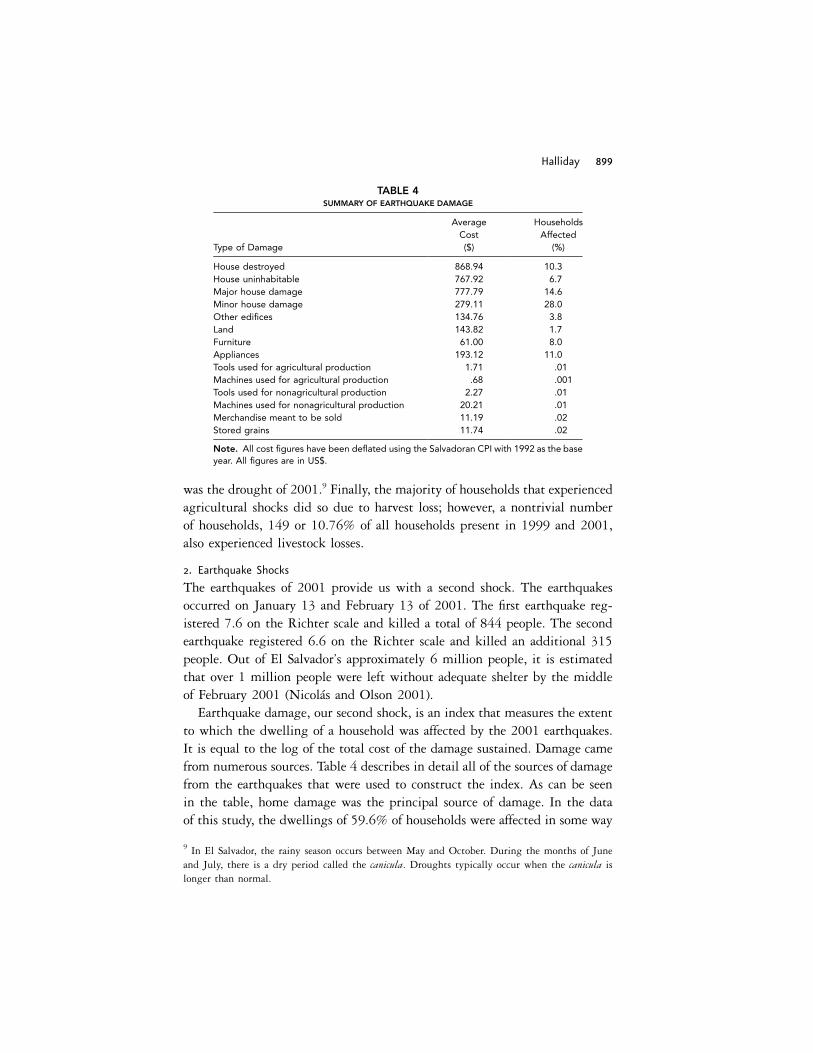
TABLE 4SUMMARY OF EARTHQUAKE DAMAGE

Type of Damage

AverageCost($)

HouseholdsAffected

(%)

House destroyed 868.94 10.3House uninhabitable 767.92 6.7Major house damage 777.79 14.6Minor house damage 279.11 28.0Other edifices 134.76 3.8Land 143.82 1.7Furniture 61.00 8.0Appliances 193.12 11.0Tools used for agricultural production 1.71 .01Machines used for agricultural production .68 .001Tools used for nonagricultural production 2.27 .01Machines used for nonagricultural production 20.21 .01Merchandise meant to be sold 11.19 .02Stored grains 11.74 .02

Note. All cost figures have been deflated using the Salvadoran CPI with 1992 as the baseyear. All figures are in US$.

was the drought of 2001.9 Finally, the majority of households that experiencedagricultural shocks did so due to harvest loss; however, a nontrivial numberof households, 149 or 10.76% of all households present in 1999 and 2001,also experienced livestock losses.

2. Earthquake Shocks

The earthquakes of 2001 provide us with a second shock. The earthquakesoccurred on January 13 and February 13 of 2001. The first earthquake reg-istered 7.6 on the Richter scale and killed a total of 844 people. The secondearthquake registered 6.6 on the Richter scale and killed an additional 315people. Out of El Salvador’s approximately 6 million people, it is estimatedthat over 1 million people were left without adequate shelter by the middleof February 2001 (Nicolas and Olson 2001).

Earthquake damage, our second shock, is an index that measures the extentto which the dwelling of a household was affected by the 2001 earthquakes.It is equal to the log of the total cost of the damage sustained. Damage camefrom numerous sources. Table 4 describes in detail all of the sources of damagefrom the earthquakes that were used to construct the index. As can be seenin the table, home damage was the principal source of damage. In the dataof this study, the dwellings of 59.6% of households were affected in some way

9 In El Salvador, the rainy season occurs between May and October. During the months of Juneand July, there is a dry period called the canicula. Droughts typically occur when the canicula islonger than normal.


by the earthquakes; 31.6% of households reported that they sustained at leastmajor damage to their homes; 17% of households reported having their homesdestroyed or rendered uninhabitable. This number coincides with the estimatethat approximately one out of six Salvadorans was left without adequate housingin the wake of the disaster, thereby suggesting that my measure of the earth-quake shock is good.10 Finally, the average cost of damage among householdswho actually sustained damage was $5,202.12. Figure 1 displays the densityof earthquake damage for each of El Salvador’s 14 departments.

C. Demographic Characteristics

I also use demographic controls. To control for household composition, Iconstruct measures of the number of household members residing at home inEl Salvador within certain age and gender brackets for all home dwellers. Inmy analysis, I only focus on the demographic composition of the householdat home in El Salvador, since I am primarily interested in controlling for theeffects of young children and elderly household members on migration de-cisions.11 Table 5 reports the descriptive statistics for my household demo-graphic variables. I report the mean and standard deviations for the numberof household members within each age/gender bracket.12 In addition, I alsoemployed data on the education of the household head; those descriptivestatistics are reported in table 1.

D. Wealth

I employ data on the household’s total landholdings; these are measured inmanzanas (1 manzana p 6,988 square meters) as a proxy for wealth.13 I usethree land measures, which are defined in table 1. The first measure, land 1,includes all the holdings of the household for which there is either a title or

10 It was not possible for the statistics from this study to be constructed from BASIS data, sincethe study was released in mid-2001 and the BASIS survey was fielded in 2002.11 The age brackets that I employ are ! 6 years, 6–10 years, 11–15 years, 16–20 years, 21–40years, 41–60 years, and 1 60 years.12 Interestingly, there are no significant differences in the gender composition of the household forhousehold members ≤ 20 years of age. However, we do observe significant differences in householdcomposition across gender for household members 120 years. In particular, we observe that thereare significantly fewer male household members residing in El Salvador who are ages 21–60. Thereason for this is that there is a relative abundance of men between these ages residing in theUnited States. What is not clear, however, is why there are significantly more men over the ageof 60. Presumably, this reflects a weakness in my data.13 An alternative proxy for wealth in the BASIS data is savings. However, only about 20% ofhouseholds have positive savings in our data in the years 1999 and 2001, whereas roughly 50%–60%of households have positive landholdings in these years, depending on which measure I use.Consequently, I felt that landholdings was a more comprehensive proxy of wealth for our sample.

Halliday 901

documents indicating the power of transfer.14 The second measure, land 2, island 1 plus any land that the household may be using with no proper legaldocumentation.15 The third measure, land 3, is the least inclusive. It onlyincludes land that has a title. Our preferred measure is land 1, as it is com-prehensive but not so comprehensive that it includes land that householdswould have difficulty selling. However, I also use the other measures as arobustness check.

E. Attrition in the BASIS Panel

An important issue to consider when working with panel data is attrition,particularly whether or not it occurs randomly. Table 2 provided some insightsinto attrition in the BASIS data. The table showed that roughly 92% of theoriginal households in 1997 survived until 2001, so that attrition was about8% over a 4-year period.16 Between 1999 and 2001, attrition was less than4%.17

A useful exercise when thinking about the potential impact that attritionmay have on estimation is to regress variables indicating survival in the panelon baseline household characteristics. This is a common exercise in the literatureon panel attrition. For more information, I refer the reader to Gottschalk,

14 Specifically, the survey asks the household whether or not they have a tıtulo or an acta detransferencia de dominio. The latter does not have the same legal guarantees as a title but can usedas a means for obtaining a title. However, due to reasons associated with poverty and lack ofeducation, many people with the acta de transferencia do not take the necessary steps to obtain atitle. I thank Alvaro Trigueros of FUSADES for clarifying this point. In my data, 2.8% of thehouseholds had land with an acta de transferencia but no title; 49.7% of the households had landwith a title.15 In my data, 11.6% of the households had land with no proper documentation.16 Unfortunately, we do not know whether households left the survey because they migrated, died,or refused to respond. However, according to economists at FUSADES, a policy-oriented thinktank in El Salvador, which shared responsibilities for administering the survey along with OhioState University, there is a common belief that migration was the primary cause of attrition. Thisaccords well with Thomas, Frankenberg, and Smith (2001), who provide direct evidence thatmigration was the primary cause of attrition in the Indonesian Family Life Survey (IFLS).17 It is informative to compare attrition in the BASIS data with that of other more commonlyused panels. In the IFLS, for example, there were three waves in 1993, 1997, and 1998. Between1993 and 1997, attrition was 6%. Interestingly, between 1993 and 1998, attrition was actuallylower at 5%. This low rate of attrition is quite remarkable given that attrition in panels fromdeveloping countries is notoriously high. It is also remarkable given that attrition in some commonlyused American panels is substantially higher. For example, in the Panel Study of Income Dynamics,attrition was about 12% between 1968 and 1969—a 1-year time period. In a more current survey,the Health and Retirement Survey, attrition was about 9% between 1991 and 1993. Thomas etal. (2001) credit a conscientious effort at tracking movers for the low rate of attrition in the IFLS.Indeed, it is reassuring that attrition in the BASIS data is lower than that of many panels fromthe developing world, and even some from the developed world, although it is substantially higherthan the IFLS.

902

903

Figure 1. Earthquake damage densities by department


TABLE 5DEMOGRAPHIC CHARACTERISTICS: AGE AND GENDER

Age Bracket Men WomenTest ofEquality

! 6 .38 .38 .02(.67) (.68) [.900]

6–10 .43 .45 .60(.69) (.69) [.437]

11–15 .41 .41 .00(.67) (.67) [.981]

16–20 .38 .37 .64(.65) (.63) [.423]

21–40 .63 .75 31.38(.75) (.69) [.000]

41–60 .45 .48 3.34(.52) (.51) [.068]

1 60 .28 .19 66.59(.47) (.41) [.000]

Note. This table reports descriptive statistics for number of house-hold members at home in El Salvador within certain age and genderbrackets for the years 1997, 1999, and 2001. Standard errors arereported in parentheses. Test of equality reports an -test of theFequality of means for men and women; p-values are reported inbrackets for each F-statistic.

Fitzgerald, and Moffit (1998) and Thomas et al. (2001). I report the resultsof this exercise in table 6.18

I have been careful to include variables indicating how prone the householdis to shocks. In the first, second, and third columns, I included the percentageof households in a municipio in 1999 and 2001 that experienced harvest andlivestock loss. In column 3, I simply included the harvest loss and livestockloss variables from 1999. Also, I included the mean of earthquake damagewithin municipios in all four columns. The logic behind this is that if pronenessto shocks is correlated with survival, then this could generate potentially seriousbiases in the estimation of the impact of shocks on migration, particularlysince the attrition literature has shown that panel survival is negatively cor-related with migration.19

The results do not reveal many significant predictors of attrition. Land-

18 Right-hand-side variables include baseline characteristics such as landholdings, a dummy in-dicating positive landholdings, the number of migrants, the head’s education, a dummy indicatingthat the household size is one, household size, the demographic variables described in Sec. II.C,and department dummies.19 Ideally, if I had had shocks from all of the baselines, I would have looked at whether or nothouseholds that received shocks were also more likely to leave the panel. This type of exercise wasonly possible using 1999 as the baseline with the agricultural shocks; it was not possible with1997 as the baseline, since the survey did not solicit information on shocks in that year. Conse-quently, I used municipio-level aggregates.

Halliday 905

TABLE 6PANEL ATTRITION

Survival1997–2001

Survival1997–2001

Survival1999–2001

Survival1997–1999

Land .003 .003 .001 .002(2.16) (2.25) (1.75) (1.45)

Dummy land 1 0 .02 .02 .03 .02(.74) (.61) (1.91) (.90)

Migrants �.01 �.01 �.01 �.01(�.67) (�.50) (�1.99) (�.94)

Head’s education .00 .00 .00 .00(.52) (.69) (.53) (.87)

Harvest loss in 1999 �.01(�.40)

Livestock loss in 1999 .01(.59)

% Harvest losses in municipio* �.07 �.03 .05(�.90) (�.32) (.82)

% Livestock losses in municipio* .14 .15 �.02(1.01) (1.06) (�.14)

Mean earthquake damage in municipio* .01 .01 .00 .01(1.50) (.88) (.11) (1.52)

Single household dummy? �.21 �.22 �.09 �.07(�1.25) (�1.24) (�.91) (�.63)

Household size �.00(�.68)

Demographics included?† No Yes Yes YesDepartment dummies? No Yes No YesF-test on agriculture shocks .73 .56 .33 .36

[.484] [.574] [.722] [.702]F-test on all shocks 1.25 .63 .26 .98

[.295] [.595] [.853] [.406]R2 .0177 .0546 .041 .0580Households 623 623 696 623

Note. The first two columns estimate the probability of surviving from 1997 to 2001. The third columnestimates the probability of surviving from 1999 to 2001, and the fourth column estimates the prob-ability of surviving from 1997 to 1999. In the first, second, and fourth columns, baseline characteristicsare from the 1997 survey. In the third column, which looks into survival from 1999 to 2001, thebaseline characteristics come from the 1999 survey. All t-statistics (presented in parentheses) arecalculated with standard errors that allow for clustering within municipios. The p-values for the F-statistics are in brackets.* For details concerning the construction of these variables, see Sec. II.E.† For details concerning the construction of these variables, see Sec. II.C or the note to table 7.

holdings is by far the most important, with households with more land beingmore likely to survive. This is not surprising, given that households with moreland are, presumably, less mobile and, hence, easier to track across survey years.In terms of the coming estimation, this is not of tremendous concern, as anypotential bias that this might cause can be mitigated by controlling for land-holdings. Turning to the shock variables, we see that the tests of joint sig-nificance on the agricultural shocks are all soundly rejected, both with andwithout the department dummies. There is some evidence, however, in the


first and last columns of table 6, that proneness to earthquake damage isweakly correlated with survival. This is potentially problematic, and I willaddress this issue in Section IV.

III. Migration, Remittances, and Risk

A. The Impact of Shocks on Migration

I begin by estimating the response of the household’s migration decision toshocks in El Salvador. Let denote the migrant stock of household h atMh,t

time t. Let denote the change in the household’s migrant stock acrossDMh,t

survey years. Let denote a vector of exogenous events that affect the house-qh,t

hold at time t that includes harvest loss, livestock loss, and earthquake damage.Next, I let denote the vector of household demographic variables that wereZh,t

described in Section II.C.20 Finally, I let denote other control variablesXh,t

such as location dummies and time dummies. This notation is held throughoutthe balance of the article.

To assess the impact of shocks on migration, I estimate the ordered responsemodel

1(DM p n) p 1(a ≤ d q � d X � d Z � � ! a )h,t n�1 1 h, t 2 h,t 3 h,t�1 h,t n

for n � {... , � 1, 0, 1, ...}, (1)

where denotes the nth ancillary parameter. I assume that is independenta �n h,t

of the vector and that it follows a logistic distribution. The(q , X , Z )h,t h,t h,t�1

advantage of the ordered-response model in equation (1) is that the additionalancillary parameters allow us to handle in a flexible manner. I am carefulDMh,t

to include lags of the household’s demographic characteristics. I do this sincemigration decisions today will affect the household’s demographic compositionin the present period.

Table 7 presents the results.21 In all five columns, we see that adverse

20 In this section, I do not address the effects of household wealth on migration. The reason forthis is that wealth has a positive effect on both northward migration (i.e., ) and southwardDM 1 0h,t

migration (i.e., ) in my data, and the parsimonious econometric model that I work withDM ! 0h,t

in this section does not allow for such nonmonotonicity. I reserve a discussion of the effects ofwealth on migration for Sec. V, when I address the role that liquidity constraints play in migrationdecisions.21 The standard errors in this table (and in all of the tables in the coming analysis) allow forclustering within municipios. I do so for two reasons. The first is that I often work with the samehousehold observed across multiple time periods. The second is that I expect many of my variables,particularly the shocks, to be spatially correlated. Accordingly, standard errors that assume thatthe data are independent and identically distributed will be incorrect. For a more thorough dis-cussion of clustering, I refer the reader to Deaton (1997). However, it is important to state thatwhile the asymptotic justification for this procedure is clear in linear models, this justification is

Halliday 907

TABLE 7MIGRATORY RESPONSES TO ADVERSE SHOCKS (NUMBER OF HOUSEHOLDS p 1,265)

(1) (2) (3) (4) (5)

Harvest loss .31 .31 .33 .27 .24(1.89) (1.87) (1.99) (1.62) (1.20)

Livestock loss .36 .36 .37 .38 .46(1.84) (1.86) (1.94) (1.95) (2.26)

Earthquake damage �.05 �.04 �.03 �.04(�2.15) (�1.80) (�1.33) (�1.44)

Earthquake damage dummy �.26(�1.54)

2001 dummy �.28 �.33 �.29 �.33 �.31(�1.55) (�1.76) (�1.58) (�1.74) (�1.44)

Demographic variables?* No No Yes Yes YesMunicipio dummies? No No No No YesDepartment dummies? No No No Yes NoF-test on agricultural shocks 8.32 8.29 9.55 8.46 8.00

[.016] [.016] [.008] [.014] [.018]F-test on all shocks 12.18 9.52 12.25 10.02 10.24

[.007] [.023] [.007] [.018] [.017]Pseudo- 2R .0078 .0072 .0137 .0177 .0599

Note. This table contains estimates from an ordered logit model where the dependent variable ismigration. All t-statistics (presented in parentheses) are calculated with standard errors that allow forclustering within municipios. The -values for the F-statistics are in brackets.p* The demographic controls that were used are indicators for the number of household members athome within certain age and gender brackets. Details are in Sec. II.C.

agricultural conditions in El Salvador had a positive effect on migration and,thus, tended to push people out of the country.22 The variables livestock lossand harvest loss are all positive and individually significant at the 10% level,and they are jointly significant at the 5% level.23 These results are consistentwith Munshi (2003), who shows that low rainfall in Mexico has a positiveimpact on migration to the United States.

less clear in nonlinear models as it would seem that correlated unobservables would fundamentallyalter the likelihood function. Nevertheless, I admonish the reader to view this clustering procedureas a “down and dirty” solution to the problem of spatial correlation.22 I also have a version of the results in this table using the Inverse Probability Weighting (IPW)Scheme developed by Moffitt, Fitzgerald, and Gottschalk (1999). This procedure corrects for aparticular form of attrition bias that occurs when the attrition is affected by observable characteristicsin the first time period but is unaffected by outcomes that occur in subsequent time periods. Theresults are very similar and are available upon request. Despite this, however, it is important notto place too much stock in the IPW results, as attrition in the current case is often being causedby migration and this type of attrition cannot be accommodated by IPW.23 I also estimated these models individually using only single years of the panel. While, notsurprisingly, the estimates are less precise, they still paint the same picture as table 7. What isinteresting about this exercise is that I know that the primary cause of agricultural shocks in 2001was a drought. Moreover, I know for certain that every harvest loss in my data in 2001 was reportedas a consequence of this drought. This then casts serious doubt on an alternative story of reversecausality in which the shock resulted as a consequence of less effort being expended on thehousehold’s farm after the departure of a family member.


The relationship between agricultural shocks and migration suggests thathouseholds that experienced agricultural losses anticipated low expected returnsto their labor at home for the foreseeable future and thus a widened north-south wage gap. Consequently, the shocks may have created additional incen-tives to send household members to the United States and disincentives forexisting migrants to return to El Salvador. In addition, as we will see, thereis some evidence that the effects of the agricultural shocks on migration areaccompanied by rises in remittances.

In contrast, table 7 shows that the earthquakes had a negative impact onmigration. The earthquake damage index is negative and significant in columns1 and 3. In column 2, I include a dummy variable indicating whether or notthe household was affected by the disaster (in lieu of the index). The dummyvariable, which tells us the average impact of the earthquakes, is negative andmoderately significant. In columns 4 and 5, I include 14 department dummiesand 167 municipio dummies. We see that the standard error on earthquakedamage is larger but that the point estimate is similar to what it was in column3.24

Excluding stories involving nonrandom assignment of the shocks (whichwe consider later), the finding that the earthquakes had a negative impact onmigration is consistent with two explanations. The first is that the earthquakescreated exigencies that caused households to retain members at home or tobring members back from the United States in order to help the family recoverfrom the disaster’s effects. The second explanation is that the earthquakes werean enormous burden on the household’s financial resources and that this pro-hibited the household from putting up the capital necessary to send membersabroad.25 In Section V, I investigate the role that liquidity constraints play inthe household’s migration decisions and in doing so attempt to disentanglethese explanations from one another.

24 It is important to address the pros and cons of the location dummies. First, using municipiodummies creates an efficiency loss, since their inclusion relies on variation in shocks within municipios.All variation in the shocks across municipios gets absorbed by the location dummies. This is desirableas it addresses any concerns about correlations between shocks and location effects. However, it isundesirable since variation that occurs across municipios is potentially useful information that doesnot get utilized, and this results in an efficiency loss. This is particularly undesirable as efficiencyis not something that is relatively abundant in shorts panels with small sample sizes and noisydata. Indeed, it may be the case that the cure is worse than the sickness. Second, El Salvador isroughly the size of Massachusetts. El Salvador is divided into 14 departments, and Massachusettsis divided into 14 counties. Consequently, I believe that it is reasonable to expect that departmentdummies may adequately control for location effects without incurring the same efficiency costsas the municipio dummies.25 “Illegal” migration to the United States from El Salvador typically requires payments to smug-glers or coyotes; this can exceed $1,500 (Menjıvar 2000).

Halliday 909

TABLE 8MARGINAL IMPACT OF SHOCKS

NorthwardMigration*

SouthwardMigration†

Agriculture shocks:Actual distribution‡ .2650 .0914Absence of shocks§ .2007 .1262% Change between rows 1 and 2 24.26 38.07

Earthquakes:§

Actual distribution‡ .2328 .10731 SD increasek .1464 .1682% Change between rows 1 and 2 37.11 56.76

Note. These are fitted probabilities calculated using estimates of eq. (1). Furtherdetail concerning the calculations can be found in the appendix.* Northward migration corresponds to the probability of .DM 1 0h,t† Southward migration corresponds to the probability of .DM ! 0h,t‡ These probabilities were calculated using the actual distribution of shocks.§ These calculations only use the fitted probabilities from 2001.k These probabilities were calculated assuming that there were no agriculturalshocks. A 1 SD increase refers to the level (not the log) of damage.

To give the reader some notion of the magnitude of these shocks, I calculatetheir marginal impacts. The results are in table 8. Detail concerning how themarginal effects were calculated can be found in the appendix. We see that,in the absence of any agricultural shocks, the probability of sending membersabroad in both years (northward migration) decreases from 0.2650 to 0.2007—a 24.26% decrease. The probability of receiving members (southward migra-tion) increases from 0.0914 to 0.1262—a 38.07% increase. Turning to theearthquakes, we see that a one standard deviation increase in the level of damagelowers the probability of northward migration in 2001 from 0.2328 to0.1464—a 37.11% change. In contrast, the probability of southward migrationgoes from 0.1073 to 0.1682—a 56.76% increase.

B. The Impact of Shocks on Remittances

We now turn to the effects of exogenous shocks in El Salvador on migrantremittances. Let denote the amount remitted by all migrants in householdrh,t

h at time t in logs, and let denote remittances in levels. Using the notationRh,t

from above for the other variables, I estimate the simple linear models

r p b � b q � b X � b Z � u , (2)h,t 0 1 h,t 2 h,t 3 h,t�1 h,t

Rh,tlog p g � g q � g X � g Z � v , (3)0 1 h,t 2 h,t 3 h,t�1 h,t( )Mh,t

to identify the effects of exogenous shocks on migrant remittances. Equation(2) tells us the impact of shocks on total migrant remittances, and equation


(3) tells us the impact of shocks on remittances per migrant. Equation (3) isof interest, as it is informative of cross-sectional risk sharing within spatiallydiversified households. In other words, it is suggestive of whether or not agiven migrant remits more when his or her family at home experiencesadversity.26

Table 9 reports the results. In the first column, we see—consistent withtable 7—that agricultural shocks are associated with higher remittances. How-ever, the inclusion of the department and municipio dummies attenuates theimpact of livestock loss and takes away the impact of harvest loss. My estimatesindicate that a livestock loss results in an increase in migrant remittances thatis on the order of 40%–60%, whereas the first column suggests that householdsthat experienced a harvest loss witnessed an increase in remittances on theorder of 40%.27 In addition, we see that the earthquakes are associated withdecreases in the total amount remitted from the United States. The elasticitiesof total migrant remittances with respect to earthquake damage in the firstthree columns are �0.11, �0.06, and �0.04, respectively. Finally, the effectsof the earthquakes shown in table 9 remain significant after the departmentdummies are added, suggesting that the marginally significant estimates inthe last two columns of table 7 were most likely the consequence of increasedimprecision due to the addition of location effects.

The basic lesson that we learn in the first three columns of table 9 is thatshocks affect total migrant remittances the same way that they affect migra-tion—although the results do become more imprecise with the addition oflocation effects. Agricultural shocks pushed people to the United States andincreased remittances, whereas the earthquakes pulled people back and de-creased remittances. In this sense, the results in table 9 reinforce those in table7.

The last two columns of table 9 report the results of estimating equation(3). In both columns, we see that the agricultural shocks had positive impactson remittances per migrant, although, when I include the department dum-mies, harvest loss is no longer significant. This is suggestive, but by no meansconclusive, that not only do households self-insure against agriculture shocksvia migration (i.e., changes in their migrant stocks across time) but householdshit by agricultural shocks insure themselves via increases in intrahouseholdtransfers (i.e., changes in the amount remitted per migrant).

26 I also estimated the remittance equation using a standard tobit model. The results are similarto the OLS results. In order to save space, the results are not reported, but they are available uponrequest. I attempted to use the Censored Least Absolute Deviations model of Powell (1984) butwas unsuccessful as the remittance data contain too much censoring.27 See n. 24 for a discussion of the pros and cons of location effects.

Halliday 911

TABLE 9RESPONSE OF HOUSEHOLD REMITTANCES TO ADVERSE SHOCKS

Dependent Variable p

RemittancesDependent Variable p

Remittances per Migrant

(1) (2) (3) (4) (5)

Harvest loss .39 .16 .05 .30 .09(1.66) (.71) (.18) (1.44) (.44)

Livestock loss .61 .43 .40 .56 .40(2.33) (1.76) (1.48) (2.30) (1.79)

Earthquake damage �.11 �.06 �.04 �.10 �.06(�3.31) (�1.77) (�1.17) (�3.25) (�2.05)

2001 dummy .82 .62 .58 .71 .56(3.79) (2.92) (2.61) (3.45) (2.81)

Demographic variables?* No Yes Yes No YesMunicipio dummies? No No Yes No NoDepartment dummies? No Yes No No YesF-test on agricultural shocks 4.09 1.93 1.11 3.63 1.78


[.000] [.076] [.311] [.001] [.062]2R .0210 .1457 .3442 .0194 .1319Number of households 1,385 1,265 1,265 1,385 1,265

Note. This table contains results from OLS regressions where the dependent variable is remittances;the -statistics are in parentheses. The p-values for the Z-statistics are in brackets.t* The demographic controls that were used are indicators for the number of household members athome within certain age and gender brackets. Details are given in Sec. II.C.

Turning to the effects of the earthquakes, we see negative and significanteffects on remittances per migrant. This is interesting as it does not suggestthat existing migrants remitted more in order to insure their families againstthe disaster’s consequences, as one would expect if the household were engagingin cross-sectional risk sharing through state-contingent transfers. One expla-nation for this coefficient is that households that were hit by the earthquakesvalued the labor of potential and existing migrants more than they valuedtheir remittances. However, a more plausible explanation is that householdsthat were more likely to be affected by the earthquakes also received fewerremittances per migrant from abroad prior to their occurrence. In other words,earthquake damage may have been nonrandomly assigned to households thatwere less likely to receive remittances. The next section discusses the impli-cations of this for the core results of table 7. It provides evidence that earthquakedamage was most likely assigned nonrandomly, but it also demonstrates thatthis was probably not responsible for the results in table 7.

This discussion highlights some of the pitfalls of OLS estimation of equations(2) and (3) to identify the impact of shocks on remittances. The first concernspotential correlation between the shocks and omitted household characteristicsresulting from nonrandom assignment. One seemingly sensible remedy forthis would be fixed effects estimation. However, while it is true that fixed


effects estimation does address many problems concerning omitted variables,it comes with considerable efficiency loss.28 Consequently, given my data, Ibelieve that the costs of fixed effects estimation greatly outweigh its benefits.29

Another pitfall associated with estimation of the remittance equations concernsmeasurement error in remittances. While it is true that measurement error independent variables will only result in asymptotic biases if it is correlated withright-hand-side variables, in finite samples it may still be problematic as itadds additional noise to our estimator that is only zero in a large sample.

IV. Alternative Explanations

In this section, I explore some alternative explanations for the previous section’sresults. I consider the possibility that migration is used to hedge risk ex anteas opposed to ex post, as well as the possibility that the shocks were assignednonrandomly to households with varying wealth levels and/or ties to the UnitedStates. I also investigate the possibility that the previous section’s results were,at least in part, the consequence of nonrandom attrition. I now discuss thesecompeting hypotheses.

Ex ante risk management. It is conceivable that the previous section’s effectsof the agricultural shocks are capturing the use of migration as an ex-ante riskcoping strategy. The reason for this is that households that are engaged inrisky agricultural activities may also engage in migration as a means of hedgingagainst risk prior to the occurrence of any shocks. This suggests that agri-cultural shocks were more likely to be assigned to households that engage inmigration as opposed to households actually migrating in response to theshock.

Nonrandom assignment to households with weak ties to the United States. Theeffects of the earthquakes on migration may be the consequence of the earth-quakes disproportionately affecting households with weaker ties to the UnitedStates as opposed to families utilizing household labor to buffer their effects.One might expect this to happen since much research has shown that migrant

28 As pointed out by Deaton (1995), addressing unobserved heterogeneity is not free. For example,one important issue concerns the role that serial correlation in the agricultural shocks plays. Ifthere is positive serial correlation (which there is in my data), demeaning results in a substantialloss of variation and thus greater imprecision. A second issue concerns the role of measurementerror. Generally, demeaning will exacerbate the role of measurement error, which, in the case ofthe agricultural shocks, should bias the estimates toward zero (see Aigner [1973] for a discussionof measurement error with binary regressors). These caveats are especially important to bear inmind given my small sample size and my short panel.29 I do have a set of fixed effects results, which are available upon request. These results, notsurprisingly, are less precise. Nevertheless, they still paint a picture similar to what we have beenseeing throughout this article.

Halliday 913

networks play important roles in the household’s migration decision in thesense that households with migrants already residing in the United States aremore likely to send additional members abroad (see Massey et al. [1987] fora discussion).30

Nonrandom assignment to poorer households. A concern similar to the previousone is that the earthquakes hit poorer households.31 This is potentially prob-lematic if households are liquidity constrained, especially given the large costof migration. As a result, it could be the case that households that were hitby the earthquakes would not have migrated irrespective of whether or notthey were affected by the earthquakes.32 While the exercises in this sectionshed some light on this issue, I provide a more thorough investigation inSection V.

Nonrandom attrition. Attrition can also play a pernicious role in the es-timation. For the agricultural shocks, we would not expect much of a bias,since the results of Section II.E did not reveal any relationship between theagricultural shocks and attrition. However, I did find some evidence thathouseholds that resided in areas that were hit hard by the earthquakes werealso more likely to survive in the panel. This is worrisome given that Thomaset al. (2001) provide evidence that migration was a major cause of attritionin the Indonesian Family Life Survey. Taken together, this suggests that sur-vivors were more likely to be hit by the earthquakes and, at the same time,less likely to migrate. This implies that my estimates of the impact of theearthquakes may be negatively biased due to nonrandom attrition.33

All of these explanations have to do with nonrandom assignment of theshocks. Consequently, investigating the plausibility of these alternative theorieswill involve testing whether or not the shocks were, in fact, randomly assigned.In addition, I can gauge the plausibility of these alternative stories by seeingif households that were affected by the shocks also had unobservable charac-teristics that made them more or less disposed to migration even in the absenceof any shocks.

To start investigating these issues, I begin by looking into whether or not

30 Similar arguments can be made for the agricultural shocks with harvest and livestock lossesbeing more likely to hit households with stronger network ties.31 This does appear to be the case in my data.32 Once again, similar arguments can be made for the agricultural shocks.33 To see this formally within the context of a linear model that is analogous to eq. (1), let

be an indicator for whether or not a household has survived in the panel froms � {0, 1} t � 1h,t

to t. A value of unity denotes survival. The direction of bias in the estimates of eq. (1) will dependon the sign of . For the reasons stated above, I do not expect there to be much of aE[s q � ]h,t h,t h,t

bias for the components of this expectation, which correspond to the agricultural shocks. However,for earthquake damage, which I denote by , I expect to see .Q E[s Q � ] ! 0h,t h,t h,t h,t


TABLE 10BASELINE HOUSEHOLD CHARACTERISTICS IN 1997 AND SHOCKS

HarvestLoss

LivestockLoss

EarthquakeDamage

Migrants in 1997 .009 .013 �.161(.80) (1.16) (�2.14)

Household size in 1997 .007 .003 �.004(1.54) (.94) (�.15)

Land in 1997 .000 �.001 �.029(.12) (�.30) (�2.71)

Head’s education in 1997 �.003 �.006 .027(�.93) (�1.99) (1.05)

Department dummies? Yes Yes YesNumber of households 1,166 1,166 1,166

Note. All t-statistics (presented in parentheses) are calculated with standard errors thatallow for clustering within municipios.

shocks are predicted by baseline household characteristics. In table 10, I regresseach of the three shocks on baseline characteristics from the 1997 survey. Thecharacteristics that I use are the household’s migrant level, landholdings, house-hold size, and the head’s education. As we can see, the only significant predictorof harvest loss is household size, with larger households being more likely toexperience subsequent losses. However, the robustness of the agricultural shocksto demographic controls in the previous section suggests that this is of littleconcern. In the second column, we see that livestock loss is only predicted bythe head’s education, with more educated households being less likely toexperience livestock loss. It is important to emphasize that subsequent agri-cultural shocks are not predicted by the baseline number of migrants in thehousehold, as would be expected if households that were engaged in riskyagricultural activities also engaged in migration to hedge against risk ex ante.In addition, this casts doubt on the alternative story, where the agriculturalshocks affected households with stronger ties to the United States. Turningto the earthquakes, we see that households with fewer migrants abroad andwith less land were more likely to be severely hit by the earthquakes. Thisraises some concern that households that were hit by the earthquakes wouldhave been less likely to migrate irrespective of the disaster, due to either thenetworks story or the liquidity constraints story.34

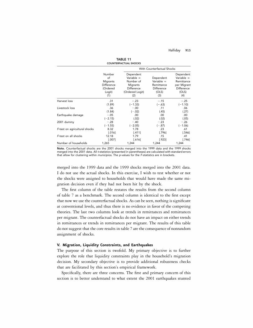
In table 11, I further investigate the possibility that the results of theprevious section are confounded by these alternative stories by looking at therelationship between “counterfactual” shocks and trends in migration andremittances. The counterfactual shocks that I employ are the 2001 shocks

34 In the next section, I include all of the significant predictors of shocks in our regressions toensure that our results are robust to nonrandom assignment. They are.

Halliday 915

TABLE 11COUNTERFACTUAL SHOCKS

Numberof

MigrantsDifference(OrderedLogit)(1)

With Counterfactual Shocks

DependentVariable pNumber ofMigrantsDifference

(Ordered Logit)(2)

DependentVariable pRemittanceDifference(OLS)(3)

DependentVariable pRemittanceper MigrantDifference(OLS)(4)

Harvest loss .31 �.23 �.15 �.25(1.89) (�1.33) (�.63) (�1.10)

Livestock loss .36 �.00 .11 .06(1.84) (�.02) (.45) (.27)

Earthquake damage �.05 .00 .00 .00(�2.15) (.02) (.02) (.05)

2001 dummy �.28 �.40 �.23 �.26(�1.55) (�2.05) (�.87) (�1.06)

F-test on agricultural shocks 8.32 1.78 .23 .61[.016] [.411] [.796] [.546]

F-test on all shocks 12.18 1.79 .15 .41[.007] [.616] [.923] [.746]

Number of households 1,265 1,244 1,244 1,244

Note. Counterfactual shocks are the 2001 shocks merged into the 1999 data and the 1999 shocksmerged into the 2001 data. All t-statistics (presented in parentheses) are calculated with standard errorsthat allow for clustering within municipios. The p-values for the F-statistics are in brackets.

merged into the 1999 data and the 1999 shocks merged into the 2001 data.I do not use the actual shocks. In this exercise, I wish to test whether or notthe shocks were assigned to households that would have made the same mi-gration decision even if they had not been hit by the shock.

The first column of the table restates the results from the second columnof table 7 as a benchmark. The second column is identical to the first exceptthat now we use the counterfactual shocks. As can be seen, nothing is significantat conventional levels, and thus there is no evidence in favor of the competingtheories. The last two columns look at trends in remittances and remittancesper migrant. The counterfactual shocks do not have an impact on either trendsin remittances or trends in remittances per migrant. The results of this tabledo not suggest that the core results in table 7 are the consequence of nonrandomassignment of shocks.

V. Migration, Liquidity Constraints, and Earthquakes

The purpose of this section is twofold. My primary objective is to furtherexplore the role that liquidity constraints play in the household’s migrationdecision. My secondary objective is to provide additional robustness checksthat are facilitated by this section’s empirical framework.

Specifically, there are three concerns. The first and primary concern of thissection is to better understand to what extent the 2001 earthquakes stunted


migration as a consequence of the disruption of migration financing. Second,I want to ensure that the effects of the earthquakes on migration are not drivenby the earthquakes disproportionately affecting poorer households that mayhave had a harder time financing migration. Finally, I also include all otherregressors from table 10 that significantly predicted shocks to ensure that theresults of table 7 are not being driven by nonrandom assignment.35

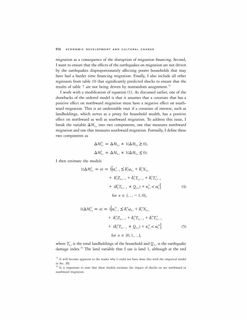
I work with a modification of equation (1). As discussed earlier, one of thedrawbacks of the ordered model is that it assumes that a covariate that has apositive effect on northward migration must have a negative effect on south-ward migration. This is an undesirable trait if a covariate of interest, such aslandholdings, which serves as a proxy for household wealth, has a positiveeffect on northward as well as southward migration. To address this issue, Ibreak the variable into two components, one that measures northwardDMh,t

migration and one that measures southward migration. Formally, I define thesetwo components as

NDM p DM # 1(DM ≥ 0),h,t h,t h,t

SDM p DM # 1(DM ≤ 0).h,t h,t h,t

I then estimate the models

S S S S1(DM p n) p 1 a ≤ d q � d X[h,t n�1 1 h,t 2 h,t

S S S 2� d Z � d T � d T3 h,t�1 4 h,t�1 5 h,t�1

S S S� (d T # Q ) � � ! a (4)]6 h,t�1 h,t h,t n

for n � {... , � 1, 0},

N N N N1(DM p n) p 1 a ≤ d q � d X[h,t n�1 1 h,t 2 h,t

N N N 2� d Z � d T � d T3 h,t�1 4 h,t�1 5 h,t�1

N N N� (d T # Q ) � � ! a (5)]6 h,t�1 h,t h,t n

for n � {0, 1, ...},

where is the total landholdings of the household and is the earthquakeT Qh,t h,t

damage index.36 The land variable that I use is land 1, although at the end

35 It will become apparent to the reader why I could not have done this with the empirical modelin Sec. III.36 It is important to note that these models estimate the impact of shocks on net northward orsouthward migration.

Halliday 917

of this section I also check to ensure that my results are robust to alternativemeasures. Here is defined as in Section III. I use lags of the household’sqh,t

landholdings to account for the fact that migration today may have a contem-poraneous impact on land transactions. In some of the specifications, I alsoinclude the household’s migrant stock and the education of the householdhead from the 1997 data (both of which significantly predicted some of theshocks in table10) as a final robustness check.37 Table 12 reports the resultsfor southward migration, and table 13 reports the results for northwardmigration.

The coefficients and for warrant some discussion. They arej jd d j � {S, N}4 5

informative regarding the impact of wealth on the household’s migrationdecision. If migration is more common among wealthier households, then wewill see that and .38 While this would be consistent with theN Sd 1 0 d ! 04 4

presence of liquidity constraints, there are certainly alternative reasons for apositive relationship between landholdings and migration.39 Consequently, apositive relationship between wealth and migration should be interpreted assuggestive, but by no means conclusive, evidence that liquidity constraintsmatter. The coefficients for allow for nonlinearities in the rela-jd j � {S, N}5

tionship between wealth and migration.The coefficients for allow the impact of an earthquake shockjd j � {S, N}6

of a given size to vary with the household’s wealth level. This interaction isimportant because the presence of liquidity constraints implies that, for ex-ample, $500 worth of damage will have a much greater impact on a household’sability to finance migration when they have no assets than when they have$10,000 worth of assets. Thus, if the earthquakes disrupted migration becausethey affected migration financing, then we would expect to see that Nd 1 06

since this would mean that the earthquakes would have stunted migration forpoorer households, who are more likely to face liquidity constraints, more thanthey stunted migration for richer households, who are less likely to face li-quidity constraints. Turning to equation (4), if the household in El Salvadorfinances the migrant’s return trip and if the earthquakes stunted migration asa consequence of liquidity constraints, then we would expect to see that

37 The impact of the 1997 migrant stock on migration in 1999 and 2001 is similar to the impactof landholdings, in the sense that it has a positive impact on northward migration and a negativeimpact on southward migration. Accordingly, to assess the impact of the migrant stock, it isessential to break the migration variable into northward and southward components.38 When the dependent variable is southward migration, a positive (negative) coefficient meansthat the variable has a negative (positive) effect on southward migration.39 For example, households with large landholdings may also be more likely to be engaged inrisky agricultural activities and, hence, more likely to use migration (either ex post or ex ante) tomitigate the impact of income shocks.


TABLE 12MIGRATORY RESPONSES TO ADVERSE SHOCKS: SOUTHWARD MIGRATION

(1) (2) (3) (4) (5)

Harvest loss .16 .08 .23 .17 .25(.65) (.31) (.90) (.67) (1.03)

Livestock loss .26 .20 .28 .27 .26(.84) (.61) (.89) (.84) (.81)

Earthquake damage .01 �.05 .01 .01 �.00(.45) (�1.96) (.37) (.21) (�.11)

Earthquake damage # land .002 .005(.34) (1.10)

Land �.07 �.02 �.09(�2.85) (�1.70) (�2.76)

Land squared .001 .002(1.78) (1.63)

2001 dummy �.78 �.76 �.76 �.72(�3.58) (�3.43) (�3.38) (�3.11)

Demographic variables?* No No No No Yes-test on agricultural shocksF 1.08 .45 1.49 1.11 1.56

[.583] [.797] [.476] [.574] [.459]-test on all shocksF 1.41 3.94 1.72 1.20 1.56

[.704] [.268] [.632] [.754] [.667]Pseudo- 2R .0124 .0033 .0173 .0148 .0336Number of households 1,265 1,265 1,265 1,265 1,265

Note. This table contains estimates from an ordered logit model where the dependent variable issouthward migration. These results use land 1 as the land variable. All t-statistics (presented in paren-theses) are calculated with standard errors that allow for clustering within municipios. The p-values forthe -statistics are in brackets.F* The demographic controls that were used are indicators for the number of household members athome within certain age and gender brackets. Details are in Sec. II.C.

since poorer households that were affected by the earthquakes wouldSd ! 06

have been less able to pay the migration costs to bring household membersback from the United States. However, since, anecdotally, we would expectthe migrant, and not the family back home, to finance return migration, wedo not expect to be that informative of the interaction between liquiditySd6

constraints and the earthquakes.In table 12, we see that household wealth, as proxied by landholdings, is

positively associated with southward migration. The estimates of are negativeSd4

and highly significant. So, we see that wealthier households are more apt tohave members migrate back from the United States.40 In columns 3 and 5 oftable 12, we see substantial evidence of nonlinearities in the wealth-migrationrelationship, as shown by the positive and significant estimates of .41 ThisSd5

40 If I use household savings in lieu of land, we see that savings is also positively associated withsouthward migration.41 The positive effects of landholdings on migration that we observe in this section are consistentwith empirical results in Hoddinott (1994) in his analysis of migration in Kenya.

Halliday 919

TABLE 13MIGRATORY RESPONSES TO ADVERSE SHOCKS: NORTHWARD MIGRATION

(1) (2) (3) (4) (5)

Harvest loss .38 .35 .40 .44 .46(1.96) (1.78) (2.02) (2.09) (2.15)

Livestock loss .38 .37 .43 .31 .32(1.83) (1.78) (2.10) (1.27) (1.32)

Earthquake damage �.09 �.08 �.07 �.07 �.07(�3.24) (�3.17) (�2.54) (�2.26) (�2.32)

Earthquake damage # land �.002 �.004 �.004(�.45) (�.76) (�.72)

Land .05 .03 .03 .03(2.33) (2.97) (2.74) (2.71)

Land squared �.001(�1.20)

2001 dummy �.00 �.04 �.09 �.09 �.09(�.02) (�.21) (�.47) (�.44) (�.41)

Migrants in 1997 .22 .22(2.65) (2.66)

Head’s education in 1997 .03(1.23)

Demographic variables?* No No Yes Yes YesF-test on agricultural shocks 8.90 8.01 11.67 8.59 9.11


[.001] [.001] [.001] [.006] [.005]Pseudo- 2R .0115 .0156 .0286 .0340 .0350Number of households 1,265 1,265 1,265 1,165 1,165

Note. This table contains estimates from an ordered logit model where the dependent variable issouthward migration. These results use land 1 as the land variable.All t-statistics (presented in paren-theses) are calculated with standard errors that allow for clustering within municipios. The p-values forthe -statistics are in brackets.F* The demographic controls that were used are indicators for the number of household members athome within certain age and gender brackets. Details are in Sec. II.C.

may be suggestive that sufficiently wealthy households do not need to rely onmigration for supplemental income or informal insurance.

Table 12 does not provide evidence that any of the shocks directly affectsouthward migration. However, it is interesting to note that, in column 2,when I exclude the year dummy, the earthquakes do have a significant effecton southward migration. Because southward migration is not that frequent inour data, this may reflect a difficulty disentangling the effects of the earthquakesfrom the year effect.42

The estimate of in table 12 is essentially zero in column 4 but is positiveSd6

42 A total of 141 households experienced southward migration in either 1999 or 2001; of these,95 households experienced southward migration in 2001. Of these 95 households, 56 experiencedsome earthquake damage. I believe that it is reasonable to expect that this small number makesit difficult to disentangle the earthquakes from the year effect in table 12.


with a t-statistic of unity in column 5 once I allow for a quadratic in land-holdings. This is interesting for two reasons. First, as argued above, if theearthquakes stunted migration as a consequence of liquidity constraints andif the household in El Salvador finances return migration (a big “if”), then wewould expect to see a negative estimate, which we do not see. Second, thepositive (but imprecise) estimate of the interaction suggests that southwardmigration as a consequence of the earthquakes was more likely for poorerhouseholds than for richer households. What this suggests is that wealthierhouseholds may have had alternative means at their disposal for buffering theshock of the earthquakes other than bringing back family members from theUnited States. Finally, this provides additional evidence that the earthquakesmay have induced southward migration, although these effects appear to beconcentrated among the poor.43

We now turn to table 13 and look at the effects of landholdings on northwardmigration. In the table, we see that the estimates of are all positive andNd4

highly significant, so that more wealth is associated with northward migration.44

Once again, the results suggest that liquidity constraints may be an importantdeterminant of households’ ability to send members abroad. However, I muststress once again that a positive relationship between migration and landholdingsis only suggestive of the presence of liquidity constraints. Completely analogousto table 12, the estimates of are all negative and significant, suggestingNd5

nonlinearities in the migration/wealth relationship. Finally, the estimates ofin columns 3, 4, and 5 are very close to zero and not significant. As arguedNd6

above, this is not what we would have expected to see if the earthquakes stuntedmigration as a consequence of liquidity constraints.45

In addition, table 13 shows that the effects of exogenous shocks on northward

43 The fact that I find some, albeit tenuous, evidence of southward migration due to the earthquakessheds an interesting light on whether the earthquakes stunted migration as a consequence of creditconstraints or increased demand for labor at home. The reason for this is that, if the only effectof the earthquakes was to disrupt migration financing, then we would not expect to see any evidenceof reverse migration due to earthquake damage.44 If I use savings in lieu of landholdings, we see that savings has a positive effect on northwardmigration.45 An important issue concerning our tests for the importance of liquidity constraints is the presenceof measurement error in both landholdings and damage. In a linear model, the classical measurementerror will result in attenuation bias, with the degree of attenuation increasing with the of the2Rshort regression of the interaction term on the remaining covariates. However, in my case, theestimate of is negative, which is not consistent with attenuation bias due to classical measurementSd6

errors. Nevertheless, the assumptions of classical measurement error are quite restrictive, and it isconceivable that a more complex form of measurement is operating in my estimation. Unfortunately,it is difficult to assess the plausibility of this scenario without alternative measures of earthquakedamage, as well as all three land measures.

Halliday 921

migration are broadly consistent with the results in table 7. We see thathouseholds that received adverse agricultural shocks were more likely to ex-perience northward migration. In addition, the table shows that householdsthat were severely affected by the earthquakes were less apt to send membersto the United States. The fact that the earthquakes are robust to the inclusionof landholdings is important, because it addresses a concern of Section IV, inwhich landholdings predicted earthquake damage.

Another concern that was raised in Section IV was that baseline migrantsalso predicted earthquake damage and that baseline education predicted live-stock loss. To address this, the fourth and fifth columns of the table addbaseline migrants and education as controls. In column 4, I add baselinemigrants. We see that, while there is a positive relationship between thehousehold’s migrant stock in 1997 and subsequent migration, which we wouldexpect if networks matter, the point estimate on earthquake damage remainsunchanged and significant. Overall, this table does not lend any support tothe alternative explanations concerning migrant networks that were raised inSection IV. In column 5, I include both baseline migrants and baseline edu-cation. While it is true that livestock loss is no longer significant, it was alsonot significant in column 4 when baseline education was not included. Con-sequently, the lower point estimate on livestock loss in columns 4 and 5probably has more to do with the sample size being reduced by 100 obser-vations than with the inclusion of baseline education.46

Finally, in table 14, I ensure that my results are robust to different measuresof landholdings. I report the coefficients on land, land squared, and the in-teraction of land and earthquake damage using the three measures of land thatare described in Section II. As can be seen in the table, my conclusions arenot affected in any way by my choice of land measure.

VI. Conclusions

This article investigated the relationship between idiosyncratic economicshocks in El Salvador and migrant flows to the United States. To accomplishthis, I utilized panel data from El Salvador that contained good measures of

46 The results in table 12 suggested that earthquake damage may not have been randomly assignedto households. One of my strategies to address this concern was to add the significant predictorsof damage as controls and check if damage was still significant. This technique comes from theliterature on treatment effects. The idea is that, provided that the outcome (migration) is inde-pendent of the treatment (damage) conditional on a set of covariates that predict treatment, theeconometrician can identify the true impact of the treatment on the outcome by regressing theoutcome on the treatment and all covariates that predict the treatment. This is what Wooldridge(2000) refers to as a “kitchen sink regression.” For an excellent overview of treatment effects usingbinary treatments, see Wooldridge (2000).


TABLE 14SOUTHWARD AND NORTHWARD MIGRATION RESULTS WITH ALTERNATIVE LAND MEASURES

Land 1 Land 2 Land 3

(1) (2) (3) (4) (5) (6)

Southward migration:Earthquake damage # land .002 �.000 .002

(.34) (�.09) (.39)Land �.07 �.02 �.08 �.02 �.07 �.03

(�2.85) (�1.70) (�2.77) (�1.38) (�2.97) (�1.78)Land squared .001 .001 .001

(1.78) (1.45) (1.74)Northward migration:Earthquake damage # land �.001 �.001 �.001

(�.22) (�.31) (�.18)Land .05 .03 .06 .03 .06 .03

(2.33) (2.38) (3.15) (1.98) (2.48) (2.45)Land squared �.001 �.001 �.001

(�1.20) (�1.84) (�1.28)

Note. This table contains regressions like those in tables 12 and 13, except that alternative landmeasureshave been used. Each regression includes the listed variables as well as the shock variables and the yeardummy. All standard errors allow for clustering within municipios; the t-statistics are in parentheses.

economic shocks and migrant flows. My results indicate that migration to theUnited States is, in part, determined by the economic conditions that prevailin El Salvador. Overall, this article paints a picture in which Salvadoran house-holds use migration as an ex post risk management strategy.

I showed that adverse agricultural conditions in El Salvador tended to pushhousehold members to the United States. In the absence of any shocks, theaverage probability that a household sends members abroad decreases by24.26%. In addition, I provided evidence that the effects of agricultural shockson migration are accompanied by increases in remittances that are on the orderof 40%–60%.

In contrast, I showed that households that were affected by the 2001 earth-quakes tended to retain members at home. A one standard deviation increasein earthquake damage lowers the average probability that a household sendssomeone to the United States by 37.11%. One explanation for this is thathouseholds retained labor at home to deal with the aftermath of the disaster.This explanation states that the labor of household members was used to bufferthe earthquake’s effects. Another explanation for this result is that Salvadoranhouseholds are liquidity constrained and that the earthquakes disrupted house-hold finances that would have otherwise been used to finance migration.

To disentangle these two explanations from one another, I investigated thenexus of migration, wealth, and the earthquakes. First, I showed that migrationis more likely for wealthier households, suggesting that liquidity constraints

Halliday 923

are important. However, I also showed that the earthquakes were just as likelyto stunt migration for wealthier households as they were for poorer households,which is not consistent with the story in which the earthquakes stuntedmigration because they disrupted migration financing.

Finally, an important topic that warrants additional work concerns the degreeof cross-sectional risk sharing that occurs between migrants and home dwellersvia remittances. This topic is challenging, as it is very difficult to identify thedirect effect that adverse shocks will have on remittances. The reason is thatshocks will affect remittances both directly and indirectly. The direct effectcorresponds to cross-sectional risk pooling. The indirect effect corresponds tohouseholds using migration as a self-insurance mechanism, which is the focusof this article. In the absence of the stringent distributional assumptions thatwould be imposed by a complicated structural model, identification would entailusing instruments that affect migration but do not affect remittances. Findingvalid instruments is likely to be difficult, if not impossible. Hence, progress onthis front most likely will need to rely on alternative methods such as structuralmodeling and, of course, better data. Another reason why this topic is challengingconcerns the role that imperfect information would play in risk pooling ar-rangements. As discussed by Rosenzweig (1988), the large distances that canseparate migrants from their families are likely to amplify the role that asym-metric information will play in intrafamily risk-sharing arrangements.

Appendix

Calculating the Marginal Impact of Shocks

I now provide the details concerning the calculation of the marginal effectsin table 9. Let denote the shock vector as defined in Section III. Let Aq qh,t h,t

have the same values for the earthquake shocks as in but have no agriculturalqh,t

disturbances. So harvest loss and livestock loss always equal zero in Al-Aq .h,t

ternatively, let have the same values for the agricultural shocks as butQq qh,t h,t

have a one standard deviation increase in the level of earthquake damage. Ithen computed the fitted probabilities from equation (1) using the specificationin column 2 of table 7 using and . Let forA Qq ,q q p (DM p nFx) x �h,t h,t h,t h,t h,t

denote the estimated probability that net migration in householdA Q{q , q , q }h,t h,t h,t

h at time t equals n evaluated at , or Then the probability ofA Qq , q q .h,t h,t h,t

northward migration (out-migration) for a household is given by

p (DM 1 0Fx) p p(DM p nFx),�h,t h,t h,t1n 0

A Qfor x � {q , q , q }, (A1)h,t h,t h,t


and the probability of southward migration (in-migration) is given by

p (DM ! 0Fx) p p(DM p nFx),�h,t h,t h,t!n 0

A Qfor x � {q , q , q }. (A2)h,t h,t h,t

The average probability of out-migration is then given by

�1p(DM 1 0Fx) p (HT) p (DM 1 0Fx), (A3)�h,t h,t h,th,t

and the average probability of in-migration is then given by

�1p(DM ! 0Fx) p (HT) p (DM ! 0Fx). (A4)�h,t h,t h,th,t

To calculate the marginal impact of the agricultural shocks, I then computedthe average probabilities in (A3) and (A4) for all households who experiencedeither a harvest loss or a livestock loss evaluated at I then calculated theseq .h,t

probabilities again for the same households under the assumption that theydid not experience any agricultural shocks, that is, using To calculate theAq .h,t

marginal impact of the earthquakes, I computed (A3) and (A4) for all house-holds in 2001 using and then again using Qq q .h,t h,t

ReferencesAigner, Dennis J. 1973. “Regression with a Binary Independent Variable Subject

to Errors of Observation.” Journal of Econometrics 1, no. 1:49–50.Besley, Timothy. 1995. “Savings, Credit, and Insurance.” In Handbook of Development

Economics, vol. 3A, ed. Jere Behrman and T. N. Srinivasan. Amsterdam: NorthHolland.

Deaton, Angus. 1992. Understanding Consumption. Oxford: Oxford University Press.———. 1995. “Data and Econometric Tools for Development Analysis.” In Handbook

of Development Economics, vol. 3A, ed. Jere Behrman and T. N. Srinivasan. Am-sterdam: North Holland.

———. 1997. The Analysis of Household Surveys: A Microeconometric Approach to De-velopment Policy. Baltimore: Johns Hopkins University Press.

Fitzgerald, John, Peter Gottschalk, and Robert Moffitt. 1998. “An Analysis of SampleAttrition in Panel Data.” Journal of Human Resources 33, no. 2:251–99.

Hoddinott, John. 1994. “A Model of Migration and Remittances Applied to WesternKenya.” Oxford Economic Papers 46, no. 3:459–76.

Massey, Douglas S., Rafael Alarcon, Jorge Durand, and Humberto Gonzalez. 1987.Return to Aztlan: The Social Process of International Migration from Western Mexico.Berkeley: University of California Press.

Menjıvar, Cecilia. 2000. Fragmented Ties: Salvadoran Immigrant Networks in America.Berkeley: University of California Press.

Moffitt, Robert, John Fitzgerald, and Peter Gottschalk. 1999. “Sample Attrition in

Halliday 925

Panel Data: The Role of Selection on Observables.” Annale d’Economie et de Statistique55–56:129–52.

MRE (Ministerio de Relaciones Exteriores). 2001. Resumen ejecutivo sobre Salvadorenosen el exterior. San Salvador: Ministerio de Relaciones Exteriores.

Munshi, Kaivan. 2003. “Networks in the Modern Economy: Mexican Migrants inthe U.S. Labor Market.” Quarterly Journal of Economics 118, no. 2:549–99.

Nicolas, Nestor A., and Richard S. Olson. 2001. “‘SUMA’ and the 2001 El SalvadorEarthquakes: An Independent External Evaluation.” Report submitted to the Pan-American Health Organization, Washington, DC, July 1, 2001.

Paulson, Anna L. 2000. “Insurance and Migration: Evidence from Thailand.” Un-published manuscript, Department of Economics, University of Chicago.

Paxson, Christina H. 1992. “Using Weather Variability to Estimate the Responseof Savings to Transitory Income in Thailand.” American Economic Review 82, no.1:15–33.

PNUD (Programa de las Naciones Unidas de Desarollo). 2001. Informe sobre desarollohumano: El Salvador New York : Programa de las Naciones Unidas de Desarollo(United Nations Development Programme).

Powell, James L. 1984. “Least Absolute Deviations Estimation of the CensoredRegression Model.” Journal of Econometrics 25, no. 3:303–25.

Ravallion, Martin, and Shubham Chaudhuri. 1997. “Risk and Insurance in VillageIndia: Comment.” Econometrica 65, no. 1:171–84.

Rosenzweig, Mark R. 1988. “Risk, Implicit Contracts, and the Family in RuralAreas of Low-Income Countries.” Economic Journal 98, no. 393:1148–70.

Rosenzweig, Mark R., and Oded Stark. 1989. “Consumption Smoothing, Migration,and Marriage: Evidence from Rural India.” Journal of Political Economy 97, no. 4:905–26.

Rosenzweig, Mark R., and Kenneth L. Wolpin. 1993. “Credit Market Constraints,Consumption Smoothing, and the Accumulation of Durable Production Assetsin Low-Income Countries: Investment in Bullocks in India.” Journal of PoliticalEconomy 101, no. 2:223–44.

Ruggles, Steven, Mathew Sobek, Trent Alexander, Catherine A. Fitch, Ronald Goe-ken, Patrica Kelly Hall, Miriam King, and Chad Ronnander. 2004. IntegratedPublic Use Microdata Series, Version 3.0. Minneapolis: Minnesota Population Center.

Thomas, Duncan, Elizabeth Frankenberg, and James P. Smith. 2001. “Lost but NotForgotten: Attrition and Follow-Up in the Indonesian Family Life Survey.” Journalof Human Resources 36, no. 3:556–92.

Townsend, Robert M. 1994. “Risk and Insurance in Village India.” Econometrica 62,no. 3:539–91.

Udry, Christopher. 1994a. “Risk and Insurance in a Rural Credit Market: An Em-pirical Investigation in Northern Nigeria.” Review of Economic Studies 61, no. 3:495–526.

———. 1994b. “Risk and Saving in Northern Nigeria.” American Economic Review85, no. 5:1287–1300.

Wooldridge, Jeffrey M. 2000. Econometric Analysis of Cross Section and Panel Data.Cambridge, MA: MIT Press.

Documents

Migration, Risk, and Liquidity Constraints in El Salvadorhalliday/Migration_EDCC.pdf · Migration, Risk, and Liquidity Constraints in El Salvador timothy halliday ... Thus, the earthquakes