Microarchitecture Sensitive Empirical Models for Compiler Optimizations

Kapil Vaswani, Matthew J. Thazhuthaveetil, Y. N. SrikantIndian Institute of Science, Bangalore{kapil,mjt,srikant}@csa.iisc.ernet.in

P. J. JosephFreescale, India

P.J.Joseph@freescale.com

Abstract

This paper proposes the use of empirical modelingtechniques for building microarchitecture sensitive mod-els for compiler optimizations. The models we build re-late program performance to settings of compiler opti-mization flags, associated heuristics and key microarchi-tectural parameters. Unlike traditional analytical model-ing methods, this relationship is learned entirely from dataobtained by measuring performance at a small numberof carefully selected compiler/microarchitecture configura-tions. We evaluate three different learning techniques in thiscontext viz. linear regression, adaptive regression splinesand radial basis function networks. We use the gener-ated models to a) predict program performance at arbitrarycompiler/microarchitecture configurations, b) quantify thesignificance of complex interactions between optimizationsand the microarchitecture, and c) efficiently search for ’op-timal’ settings of optimization flags and heuristics for anygiven microarchitectural configuration.

Our evaluation using benchmarks from the SPECCPU2000 suits suggests that accurate models (< 5% av-erage error in prediction) can be generated using a reason-able number of simulations. We also find that using com-piler settings prescribed by a model-based search can im-prove program performance by as much as 19% (with anaverage of 9.5%) over highly optimized binaries.

1. Introduction

High performance processors and optimizing compil-ers are arguably the two most critical building blocks ofhigh performance computing systems. With access tolarge parts of program code and abundant computationalresources, modern optimizing compilers employ sophisti-cated program analyzes to identify optimization opportu-nities and drive several code and data transformations thatcan improve program performance. On their part, proces-sors rely on a number of aggressive microarchitectural opti-mizations that exploit dynamic properties of code and data

and speedup programs by facilitating the execution of in-structions in parallel. It is therefore not surprising thatmost compiler and micro-architectural optimizations inter-act with each other i.e. the effect of an optimization is de-termined by the presence of other optimizations and cannotbe measured in isolation. Understanding the nature of theseoptimizations and their interactions is critical for problemssuch as phase ordering[2, 10] and important for the designof efficient compilers in general.

Despite several research efforts, an accurate and scalablemethod of characterizing compiler optimizations and theirinteractions remains elusive. The difficulty in developingsuch methods stems from the sheer complexity of moderncompilers and hardware. A typical compiler consists of alarge number of potentially interacting optimizations, eachparametrized by a number of independent heuristics, thresh-olds and flags. Moreover, optimizations such as compiler-directed prefetching, procedure inlining and loop unrollinginvolve complex cost-benefit trade-offs that cannot be ac-curately captured by simple models. Modern superscalarprocessors add to the complexity of analysis by employingseveral hard-to-analyze dynamic optimizations of their own- out-of-order execution, branch prediction and multi-levelcaching are prime examples of such optimizations.

Although the dynamics of interactions between opti-mizations are not well understood, existing compilers arenot entirely oblivious to the presence of these interactions.In fact, most compiler optimizations rely on carefully de-signed heuristics based on some abstraction or model of theunderlying hardware, to maximize the benefits of the opti-mization and guard against negative interactions that mayhurt performance. Although not without its advantages, theuse of such hardware models and manually designed com-piler heuristics has the following key drawbacks.

• Unknown interactions. In the absence of accuratemethods for quantifying compiler and hardware in-teractions, the compiler writer must speculate on themagnitude and nature of interactions and identify in-teractions that are most likely to effect performance.Any oversight or error on the compiler writer’s partmay result in heuristics that focus on the wrong inter-

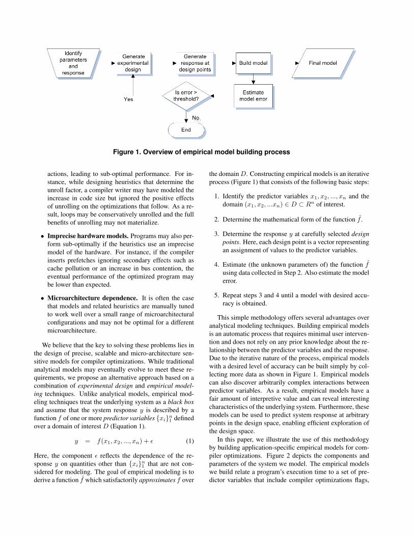
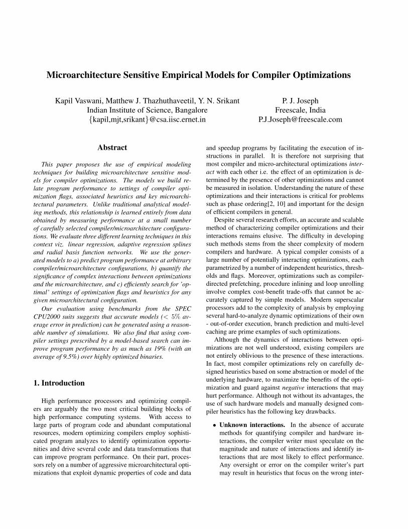
Figure 1. Overview of empirical model building process

actions, leading to sub-optimal performance. For in-stance, while designing heuristics that determine theunroll factor, a compiler writer may have modeled theincrease in code size but ignored the positive effectsof unrolling on the optimizations that follow. As a re-sult, loops may be conservatively unrolled and the fullbenefits of unrolling may not materialize.

• Imprecise hardware models. Programs may also per-form sub-optimally if the heuristics use an imprecisemodel of the hardware. For instance, if the compilerinserts prefetches ignoring secondary effects such ascache pollution or an increase in bus contention, theeventual performance of the optimized program maybe lower than expected.

• Microarchitecture dependence. It is often the casethat models and related heuristics are manually tunedto work well over a small range of microarchitecturalconfigurations and may not be optimal for a differentmicroarchitecture.

We believe that the key to solving these problems lies inthe design of precise, scalable and micro-architecture sen-sitive models for compiler optimizations. While traditionalanalytical models may eventually evolve to meet these re-quirements, we propose an alternative approach based on acombination of experimental design and empirical model-ing techniques. Unlike analytical models, empirical mod-eling techniques treat the underlying system as a black boxand assume that the system response y is described by afunction f of one or more predictor variables {xi}n

1 definedover a domain of interest D (Equation 1).

y = f(x1, x2, ..., xn) + ε (1)

Here, the component ε reflects the dependence of the re-sponse y on quantities other than {xi}n

1 that are not con-sidered for modeling. The goal of empirical modeling is toderive a function f̂ which satisfactorily approximates f over

the domain D. Constructing empirical models is an iterativeprocess (Figure 1) that consists of the following basic steps:

1. Identify the predictor variables x1, x2, ..., xn and thedomain (x1, x2, ...xn) ∈ D ⊂ Rn of interest.

2. Determine the mathematical form of the function f̂ .

3. Determine the response y at carefully selected designpoints. Here, each design point is a vector representingan assignment of values to the predictor variables.

4. Estimate (the unknown parameters of) the function f̂using data collected in Step 2. Also estimate the modelerror.

5. Repeat steps 3 and 4 until a model with desired accu-racy is obtained.

This simple methodology offers several advantages overanalytical modeling techniques. Building empirical modelsis an automatic process that requires minimal user interven-tion and does not rely on any prior knowledge about the re-lationship between the predictor variables and the response.Due to the iterative nature of the process, empirical modelswith a desired level of accuracy can be built simply by col-lecting more data as shown in Figure 1. Empirical modelscan also discover arbitrarily complex interactions betweenpredictor variables. As a result, empirical models have afair amount of interpretive value and can reveal interestingcharacteristics of the underlying system. Furthermore, thesemodels can be used to predict system response at arbitrarypoints in the design space, enabling efficient exploration ofthe design space.

In this paper, we illustrate the use of this methodologyby building application-specific empirical models for com-piler optimizations. Figure 2 depicts the components andparameters of the system we model. The empirical modelswe build relate a program’s execution time to a set of pre-dictor variables that include compiler optimizations flags,

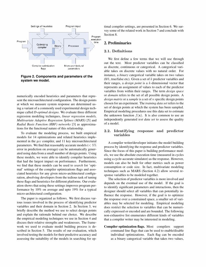
Figure 2. Components and parameters of thesystem we model.

numerically encoded heuristics and parameters that repre-sent the microarchitectural configuration. The design pointsat which we measure system response are determined us-ing a variant of a commonly used experimental design tech-nique called D-optimal designs. We evaluate three differentregression modeling techniques, linear regression models,Multivariate Adaptive Regression Splines (MARS) [5] andRadial Basis Function (RBF) networks [3] as approxima-tions for the functional nature of this relationship.

To evaluate the modeling process, we built empiricalmodels for 14 optimizations and related heuristics imple-mented in the gcc compiler, and 11 key microarchitecturalparameters. We find that reasonably accurate models (< 5%error in prediction on average) can be automatically gener-ated using data from a small number of design points. Usingthese models, we were able to identify compiler heuristicsthat had the largest impact on performance. Furthermore,we find that these models can be used to search for ’opti-mal’ settings of the compiler optimizations flags and asso-ciated heuristics for any given micro-architectural configu-ration, absolving developers from the tedious task of tuningthese flags and heuristics for different platforms. Our evalu-ation shows that using these settings improves program per-formance by 10% on average and upto 19% for a typicalmicro-architectural configuration.

The paper is organized as follows. We first discuss var-ious issues involved in the process of identifying predictorvariables and their domain in Section 2. In Section 3, webriefly describe the method we use to select design pointsand explain the rationale behind our choice. We describethe empirical modeling techniques we use in Section 4 anddiscuss their relative strengths and weaknesses. The frame-work we used to evaluate model building process is de-scribed in Section 5. The results of our evaluation, whichinvolved testing the models for their predictive accuracy andassessing the suitability of the models in searching for op-

timal compiler settings, are presented in Section 6. We sur-vey some of the related work in Section 7 and conclude withSection 8.

2. Preliminaries

2.1. Definitions

We first define a few terms that we will use throughout the text. Most predictor variables can be classifiedas discrete, continuous or categorical. A categorical vari-able takes on discrete values with no natural order. Forinstance, a binary categorical variable takes on two values(0/1, true/false etc). Given a set of k predictor variables andtheir ranges, a design point is a k-dimensional vector thatrepresents an assignment of values to each of the predictorvariables from within their ranges. The term design spaceor domain refers to the set of all possible design points. Adesign matrix or a sample is a set of n specific design pointschosen for an experiment. The training data set refers to theset of design points at which the system has been sampled.Empirical modeling procedures use this data set to estimatethe unknown function f(x). It is also common to use anindependently generated test data set to assess the qualityof a model.

2.2. Identifying response and predictorvariables

A compiler writer/developer initiates the model buildingprocess by identifying the response and predictor variables.Since the focus of this paper is building performance mod-els, we use the absolute execution time (measured in cyclesusing a cycle-accurate simulator) as the response. However,models can also be built for other metrics such as powerconsumption or code size. In fact, multivariate modelingtechniques such as MARS (Section 4.2) allow several re-sponse variables to be modeled together.

The selection of predictor variables is more involved anddepends on the eventual use of the model. If the goal isto identify significant parameters and interactions, then thedesigner should select all variables that can potentially in-fluence the response. However, if the goal is to optimizethe response over a constrained space, a smaller set of vari-ables may be selected for modeling. Empirical modelingdoes restrict the selection to variables that can be numeri-cally expressed or encoded and are bounded. The followingnon-exhaustive list enumerates different kinds of variablesthat a compiler writer may be interested in modeling.

Compiler optimization flags. Most compilers supportcommand line flags that can be used to enable/disableindividual optimizations. Each flag can be encodedas a binary categorical variable that takes two values,

0/1, which indicate whether the optimization isdisabled/enabled.

Microarchitectural parameters. Parameters such asbuffer sizes, cache sizes, number of functional units,number of registers, latencies etc. are naturallyexpressed as ordinary discrete variables whereasothers including inorder/out-of-order issue can berepresented as binary categorical variables.

Compiler heuristics. We find that several compiler opti-mizations rely on one or more numeric parameters thatare used to determine where and how to apply the opti-mization. Consider the following optimizations in gcc:

• Function inlining and loop unrolling: Inlining isdriven by a number of threshold based heuristicssuch as the maximum number of instructions inthe callee and the maximum permissible increasein code size of the caller; these heuristics helpprotect against thrashing in the instruction cache.The inliner also uses an estimate of the relativecost of a call to exclude call sites that are un-likely to yield significant benefits. A similar setof thresholds governs loop unrolling and peeling.

• Trace scheduling: This optimization relies heav-ily on heuristics to determine how traces areformed. For instance, the optimizer decides toextend an existing trace only if the followingbranch has a bias greater than a threshold. Theoptimizer can also be tuned to limit the increasein code size due to tail duplication.

Apart from these numeric parameters, other non-numericvariables that influence the behavior of an optimization mayalso be considered for modeling. For instance, a set of pri-ority functions [16] can be represented by a single categori-cal variable. A complete list of variables we chose to modelis presented in Section 5.

2.3. Defining predictor variable ranges, lev-els and transformations

The compiler writer/developer is also required to spec-ify the operating range of values for each non-categoricalpredictor variable. Since empirical models are known to beinaccurate around the edges of the chosen design space, itis advisable to select a range of values that is slightly widerthan the operating ranges. Furthermore, our experimentsshow that varying each predictor variables at as many lev-els as possible tends to increase the accuracy of the result-ing models. However, certain predictor variables such ascache sizes and buffer sizes that can only vary in powers of2. Such variables can be transformed into linear predictorvariables using functions such as log or inverse.

3. Design of Experiments

Having identified the response and the predictor vari-ables, the next step in empirical model building is to selecta set of design points in the domain of interest at whichthe response will be measured. Such a selection is neces-sitated because the total number of points in the domain isusually very large (exponential in the number of predictorvariables) and measuring the response at all points is in-feasible. It is important to note that the choice of designpoints is closely related to the accuracy and cost of buildingempirical models. For instance, models generated using aset of design points that are clustered in one region are un-likely to be accurate over the entire domain. Experimentaldesign techniques address this problem by selecting designpoints based on certain criteria; the resulting designs aremore amenable for analysis and likely to generate modelswith higher accuracy. For reasons discussed below, we usean experimental design technique known as D-optimal de-sign [11] for selecting design points.

A D-optimal design of a specified size can be generatedby first generating a set of candidate design points (eitherrandomly or through methods such as latin hypercube sam-pling) and then solving the following optimization problem.

D-optimal design problem. Given a set of m candidatedesign points Z (an m × k matrix, where k is the numberof predictor variables), choose a set of n design points (ann × k matrix X) from Z such that the determinant of theinformation matrix det(X ′X) is maximized.

It can be shown that maximizing the criteria det(X ′X)is roughly equivalent to increasing the confidence in the em-pirical models generated using the design. Algorithms forgenerating D-optimal designs are available in most statisti-cal packages. D-optimal designs are extensible i.e. an ex-isting D-optimal design can be easily augmented with ad-ditional design points. This is useful in scenarios where aninitial design proves to be insufficient and additional datais required. Furthermore, D-optimal designs are compatiblewith almost all empirical modeling techniques.

4. Empirical Modeling Techniques

The goal of empirical modeling is to learn the relation-ship between the response and the predictor variables usingsamples from the system. We first describe three techniquesthat are commonly used to accomplish this task. We thenaddress the problem of overfitting, which commonly occursin over-trained empirical models.

4.1. Linear regression models

Linear regression belongs to a class of global, paramet-ric regression techniques where the nature of the functionalrelationship between the response and the predictor vari-ables is assumed to be known a priori and the specific pa-rameters of the relationship are determined from the data.In the specific instance of linear models, we assume that theresponse y is linearly related to predictor variables {xi}n

1 .In its simplest form, a linear regression model is representedas follows:

y = β0 +n∑

i=1

βixi + ε

Here, the coefficients {βi}n0 , also known as partial regres-

sion coefficients, reflect the effect or significance of the cor-responding predictor variable on the response. Linear mod-els can easily be extended to model interactions betweenpredictor variables. For instance, the following model in-cludes terms that represent two-factor interactions.

y = β0 +n∑

i=1

βixi +n∑

i=1

n∑j=i

βijxixj + ε (2)

Building linear models. Linear regression models are rela-tively easy and quick to compute. Given a linear model withk terms and a training data set consisting of a design matrixX and the response vector y, the least squares estimates ofthe partial regression coefficients β̂ = (β0, β1, . . . , βk−1)are computed as follows:

β̂ = (X′X)−1X′y (3)

This estimate is known as the least squares estimate becauseit minimizes the sum of squares training error SSE.

SSE =p∑

i=1

(f̂(xi)− yi)2 (4)

where p is the number of samples in the training data set.

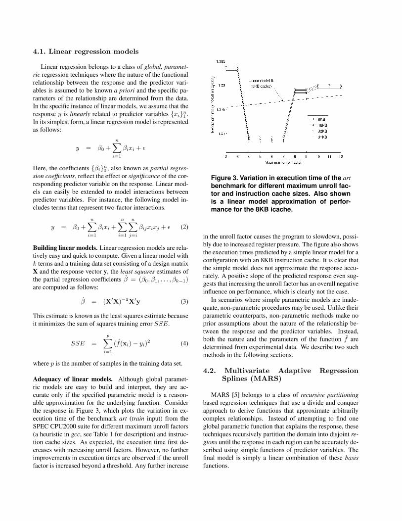
Adequacy of linear models. Although global paramet-ric models are easy to build and interpret, they are ac-curate only if the specified parametric model is a reason-able approximation for the underlying function. Considerthe response in Figure 3, which plots the variation in ex-ecution time of the benchmark art (train input) from theSPEC CPU2000 suite for different maximum unroll factors(a heuristic in gcc, see Table 1 for description) and instruc-tion cache sizes. As expected, the execution time first de-creases with increasing unroll factors. However, no furtherimprovements in execution times are observed if the unrollfactor is increased beyond a threshold. Any further increase

Figure 3. Variation in execution time of the artbenchmark for different maximum unroll fac-tor and instruction cache sizes. Also shownis a linear model approximation of perfor-mance for the 8KB icache.

in the unroll factor causes the program to slowdown, possi-bly due to increased register pressure. The figure also showsthe execution times predicted by a simple linear model for aconfiguration with an 8KB instruction cache. It is clear thatthe simple model does not approximate the response accu-rately. A positive slope of the predicted response even sug-gests that increasing the unroll factor has an overall negativeinfluence on performance, which is clearly not the case.

In scenarios where simple parametric models are inade-quate, non-parametric procedures may be used. Unlike theirparametric counterparts, non-parametric methods make noprior assumptions about the nature of the relationship be-tween the response and the predictor variables. Instead,both the nature and the parameters of the function f̂ aredetermined from experimental data. We describe two suchmethods in the following sections.

4.2. Multivariate Adaptive RegressionSplines (MARS)

MARS [5] belongs to a class of recursive partitioningbased regression techniques that use a divide and conquerapproach to derive functions that approximate arbitrarilycomplex relationships. Instead of attempting to find oneglobal parametric function that explains the response, thesetechniques recursively partition the domain into disjoint re-gions until the response in each region can be accurately de-scribed using simple functions of predictor variables. Thefinal model is simply a linear combination of these basisfunctions.

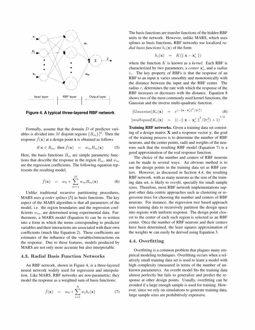
Figure 4. A typical three-layered RBF network

Formally, assume that the domain D of predictor vari-ables is divided into M disjoint regions {Rm}M

1 . Then theresponse f̂(x) at a design point x is obtained as follows

if x ∈ Rm, then f̂(x) = wmBm(x) (5)

Here, the basis functions Bm are simple parametric func-tions that describe the response in the region Rm, and wm

are the regression coefficients. The following equation rep-resents the resulting model.

f̂(x) = w0 +M∑

m=1

wmBm(x) (6)

Unlike traditional recursive partitioning procedures,MARS uses q-order splines [5] as basis functions. The keyaspect of the MARS algorithm is that all parameters of themodel, i.e. the region boundaries and the regression coef-ficients wm, are determined using experimental data. Fur-thermore, a MARS model (Equation 6) can be re-writteninto a form in which the terms corresponding to predictorvariables and their interactions are associated with their owncoefficients (much like Equation 2). These coefficients areestimates of the influence of the variables/interactions onthe response. Due to these features, models produced byMARS are not only more accurate but also interpretable.

4.3. Radial Basis Function Networks

An RBF network, shown in Figure 4, is a three-layeredneural network widely used for regression and interpola-tion. Like MARS, RBF networks are non-parametric; theymodel the response as a weighted sum of basis functions:

f̂(x) = w0 +N∑

i=1

wihi(x) (7)

The basis functions are transfer functions of the hidden RBFunits in the network. However, unlike MARS, which usessplines as basis functions, RBF networks use localized ra-dial basis functions hi(x) of the form

hi(x) = K(‖ x− xic ‖)

where the function K is known as a kernel. Each RBF ischaracterized by two parameters, a center xi

c, and a radiusri. The key property of RBFs is that the response of anRBF to an input x varies smoothly and monotonically withthe distance between the input and the RBF center. Theradius ri determines the rate with which the response of theRBF increases or decreases with the distance. Equation 8shows two of the most commonly used kernel functions, theGaussian and the inverse multi-quadratic function.

[Gaussian]Ki(x) = e(−‖x−xic‖

2/2r2

i ) (8)

[multiquad]Ki(x) = ((−‖ x− xic ‖

2/2r2

i ) + 1)1/2

Training RBF networks. Given a training data set consist-ing of a design matrix X and a response vector y, the goalof the training process is to determine the number of RBFneurons, and the center points, radii and weights of the neu-rons such that the resulting RBF model (Equation 7) is agood approximation of the real response function.

The choice of the number and centers of RBF neuronscan be made in several ways. An obvious method is touse the design points in the training data set as RBF cen-ters. However, as discussed in Section 4.4, the resultingRBF network, with as many neurons as the size of the train-ing data set, is likely to overfit, specially for small samplesizes. Therefore, most RBF network implementations sup-port other data centric approaches such as clustering or re-gression trees for choosing the number and centers of RBFneurons. For instance, the regression tree based approachuses training data to recursively partition the design spaceinto regions with uniform response. The design point clos-est to the center of each such region is selected as an RBFcenter. Once the number of RBF neurons and their centershave been determined, the least squares approximation ofthe weights w can easily be derived using Equation 3.

4.4. Overfitting

Overfitting is a common problem that plagues many em-pirical modeling techniques. Overfitting occurs when a rel-atively small training data set is used to learn a model withhigh complexity (measured in terms of the number of un-known parameters). An overfit model fits the training dataalmost perfectly but fails to generalize and predict the re-sponse at other design points. Usually, overfitting can beavoided if a large enough sample is used for training. How-ever, since we rely on simulations to generate training data,large sample sizes are prohibitively expensive.

# Parameter Description LowValue

HighValue

# levels

1 -finline-functions Inline simple functions into their callers 0 1 22 -funroll-loops Unroll loops whose number of iterations can be determined statically or at loop

entry0 1 2

3 -fschedule-insns2 Reorder instructions to eliminate execution stalls. Perform before and afterregister allocation

0 1 2

4 -floop-optimize Perform simple loop optimizations such as moving constant expressions, sim-plify test conditions etc.

0 1 2

5 -fgcse Perform GCSE pass, also perform constant and copy propagation 0 1 26 -fstrength-reduce Perform loop strength reduction and elimination of induction variables 0 1 27 -fomit-frame-pointer Do not keep the frame pointer in a register if not required 0 1 28 -freorder-blocks Reorder block to reduce number of taken branches and improve code locality 0 1 29 -fprefetch-loop-arrays Generate prefetch instructions in loops that access large arrays 0 1 210 max-inline-insns-auto Maximum number of instructions (in GCC IR) in a single function for it to be

considered for inlining50 150 11

11 inline-unit-growth Maximum overall growth of a compilation unit due to inlining 25 75 1112 inline-call-cost Cost of a call relative to a simple computation; used to identify beneficial call

sites12 20 9

13 max-unroll-times Maximum number of times a single loop can be unrolled 4 12 914 max-unrolled-insns Maximum number of instructions a loop can have for it to be considered for

unrolling100 300 21

Table 1. Compiler flags and heuristics considered for empirical modeling. Also listed are the pa-rameter ranges and the number of levels for each parameter. All compiler parameters are linearlytransformed to a scale -1 to 1 for modeling.

Overfitting can also be avoided by constraining modelcomplexity using metrics that estimate the ability of a modelto generalize. Over the years, many such metrics have beendeveloped. One such metric is the Bayesian InformationCriteria (BIC) defined by the following relation.

BIC =p + (ln(p)− 1)γ

p(p− γ)SSE (9)

Here, SSE is the sum of squares error on the training data(Equation 4), p is the number of samples in the trainingdata set and γ is the number of parameters in the model. Inessence, the BIC is a version of the SSE that also accountsfor the model’s complexity. Other metrics such as the GCV(Generalized Cross Validation) are also commonly used.

5. Experimental Framework

We now describe the framework we used to test themodel building procedure and evaluate the accuracy,scalability and utility of the performance models.

Parameter selection. We model a set of optimizationsin the gcc compiler infrastructure (version 4.0.1). Thechoice of the compiler was governed by two factors - itswidespread use, and support for a backend for which a val-idated simulator was available. Table 1 enumerates the setof 14 optimizations and associated heuristics we chose tomodel, their ranges (defined by the low and high values)and the number of levels. All optimization flags are binary

encoded categorical variables, whereas the 5 heuristics arenumeric variables that control inlining and unrolling.

The microarchitectural parameters we considered formodeling are listed in Table 2 along with the respectiveranges and levels. The list primarily comprises of pa-rameters related to the processor core and the memorysubsystem. Previous studies [8] have shown that many ofthese parameters have a high influence on performance.Furthermore, the microarchitectural design space definedby these parameter ranges covers the configurations of mostmodern superscalar processors. Two of these parametersdeserve special mention. Since the number of functionalunits is usually dependent on the issue width, we use theissue width parameter to determine the functional unitconfiguration. Also, the branch predictor size parameterrefers to the size of the predictor tables in a combinedbranch predictor consisting of a bimodal predictor and a2-level predictor of equal sizes. We note that this selectionof compiler optimizations and microarchitectural parame-ters is by no means exhaustive. However, this selection islarge enough to demonstrate the efficacy of our approach.Modeling this set of parameters is already beyond thecapabilities of traditional analytical methods [21].

Generating experimental designs. We used the AlgDe-sign package in the R statistical tool to generate D-optimaldesigns for the space defined by 25 parameters. Weconservatively chose a design of size 400 as our trainingdata set and an independently generated design of size 100

# Parameter Low High #Value Value Levels

15 Issue width 2 4 216 Branch predictor size* 512 8192 517 Register update unit size* 16 128 418 Instruction cache size* 8KB 128KB 519 Data cache size* 8KB 128KB 520 Data cache associativity 1 2 221 Data cache latency 1 3 322 Unified l2 cache size* 256KB 8MB 623 Unified l2 cache associativity* 1 8 424 Unified l2 cache latency 6 16 1125 Memory latency 50 150 21

Table 2. Micro-architectural parameters con-sidered for empirical modeling. All parame-ters marked ”*” are log transformed.

as our test data set.

Generating program binaries. The first step in measuringprogram performance at a given design point is to generatea program binary that corresponds to the settings ofvariables at the design point. This is achieved by compilingthe program with a set of command line flags and param-eters determined by the design point. However, certainmicroarchitectural parameters may need special treatment.For instance, the machine description used by the compilerto guide instruction scheduling must be consistent withthe functional unit configuration used at the design point.In our setup, we compiled several versions of gcc for theAlpha backend, one for every possible functional unitconfiguration and use an appropriate version to compile theprogram.

Simulation methodology. We use a modified version ofSimplescalar, a detailed, cycle accurate processor simulatorfor the Alpha architecture, to measure the response (execu-tion time in cycles) at selected design points. Our simulatormodels the memory system in detail. Specifically, the simu-lator accurately models store buffers, buses and the DRAM.

However, measuring program performance using de-tailed cycle accurate simulation is expensive. The prob-lem is further exacerbated for the following reasons: a) thenumber of simulations required to build models (the size ofthe training data set) is likely to be large, and b) each de-sign point may correspond to a different program binary.As a result, IPC is no longer a valid performance metricand traditional simulation time reduction techniques suchas Simpoint [14] cannot be used. In this paper, we addressthis problem by using SMARTS based methodology [19]for simulation. SMARTS relies on statistical sampling toreduce simulation time by several orders of magnitude, al-lowing programs to be simulated to completion. Further-

Benchmark-Input Linear model MARS RBF-RT164.gzip-graphic 4.44 3.17 2.90175.vpr-route 7.69 3.78 1.84177.mesa 20.15 8.78 7.31179.art 26.44 14.20 4.63181.mcf 11.25 4.85 3.99255.vortex-lendian1 9.69 6.95 5.15256.bzip2-graphic 4.81 2.80 3.02Average 12.07 6.35 4.13

Table 3. Average prediction error obtainedusing three modeling techniques.

more, SMARTS provides estimates of the potential error inmeasurement due to sampling. These estimates can be usedto tune the sampling parameters and repeat the simulationuntil a desired level of accuracy is obtained.

For the purpose of this study, we chose the samplingwindow size (# number of instructions sampled in onewindow) of 1000 and a sampling interval of 1000 (1 inevery 1000 windows is sampled). Our experiments showthat this choice of sampling parameters results in < 1%error (with 99.7% confidence) in estimating execution timefor all programs we tested. This reduces the simulationtime from several months to a few hours.

Building models. We use the iterative procedure illus-trated in Figure 1 to build models for a given program-inputpair. The linear models we build incorporate individualeffects between parameters and two-factor interactions be-tween them. The cost of building a large training data setprevents us from including higher order interactions. Weconstruct the MARS models using the polspline package inR, which supports the use of the GCV measure to avoidoverfitting. The RBF network models we build rely on re-gression trees [12] for choosing the number and centers ofRBF neurons. We evaluated several kernel functions andfound that models based on the multi-quadratic kernel to bethe most accurate. The linear and RBF modeling proceduresalso use the BIC criteria to avoid overfitting.

6. Experimental Results

6.1. Model Diagnostics

We estimate the accuracy of the program-specific mod-els by using the models to predict the performance at thedesign points in an independently generated test data set ofsize 100. Table 3 shows the average percentage error inprediction achieved by the three modeling techniques for 7programs from the SPEC CPU2000 suite. Clearly, the mod-els based on RBF networks outperform the other modelingtechniques across all programs, achieving an average errorof < 5% for all programs. Also note that the MARS models

Figure 5. Effect of size of the training data set on model accuracy for benchmarks from the SPECCPU2000 suite. The black line indicates the average error µ and the gray area represents the errorvariance σ.

compare well with the RBF network models for some of theprograms we tested. However, linear models are plagued byhigh errors, which suggests that program performance maynot vary linearly over large regions of the design space.

Figure 5 illustrates the effect of the training data set sizeon the accuracy of RBF network models. As expected, theaverage error in prediction tends to decrease with increasingsample sizes. Most exceptions to this rule occurs when verysmall sample sizes (< 100) are used. We observe that thenumber of samples required for the error to stabilize belowthe threshold of 5% varies from program to program. Fora majority of the programs, this error threshold is reachedbetween 100-200 simulation runs. Also note that the vari-ance in error (indicated by the gray region which representsµ ± σ) also decreases with increasing sample sizes. How-ever, increasing the sample size beyond this threshold yieldsincremental benefits.

Figure 6 throws more light on the predictive capabilitiesof the RBF models. Here, we plot the actual execution timevs. the predicted execution time at 100 design points in thetest data set for three programs with relatively high error.

We observe that all models capture high level trends in per-formance and no outliers are observed.

6.2. Interpreting models

Although RBF models prove to be more accurate thanthe MARS models, they suffer from the lack of inter-pretability. Therefore, MARS models may in fact be pre-ferred in cases where they are sufficiently accurate. Asaforementioned, MARS models can be represented in aform in which each predictor variable/interaction is asso-ciated with a single coefficient, which represents its signif-icance over the entire design space. Table 4 shows the keyparameters/interactions and their coefficients as inferredfrom the simplified form of the MARS models for program-input pairs we tested. In these models, the co-efficient valueof a predictor variable/interaction is equal to one-half thechange in execution time (measured in billions on cycles)caused by changing the variable(s) from their low to highvalue. This listing reveals several interesting insights. First,we note that the micro-architectural parameters and inter-actions dominate program performance, whereas compiler

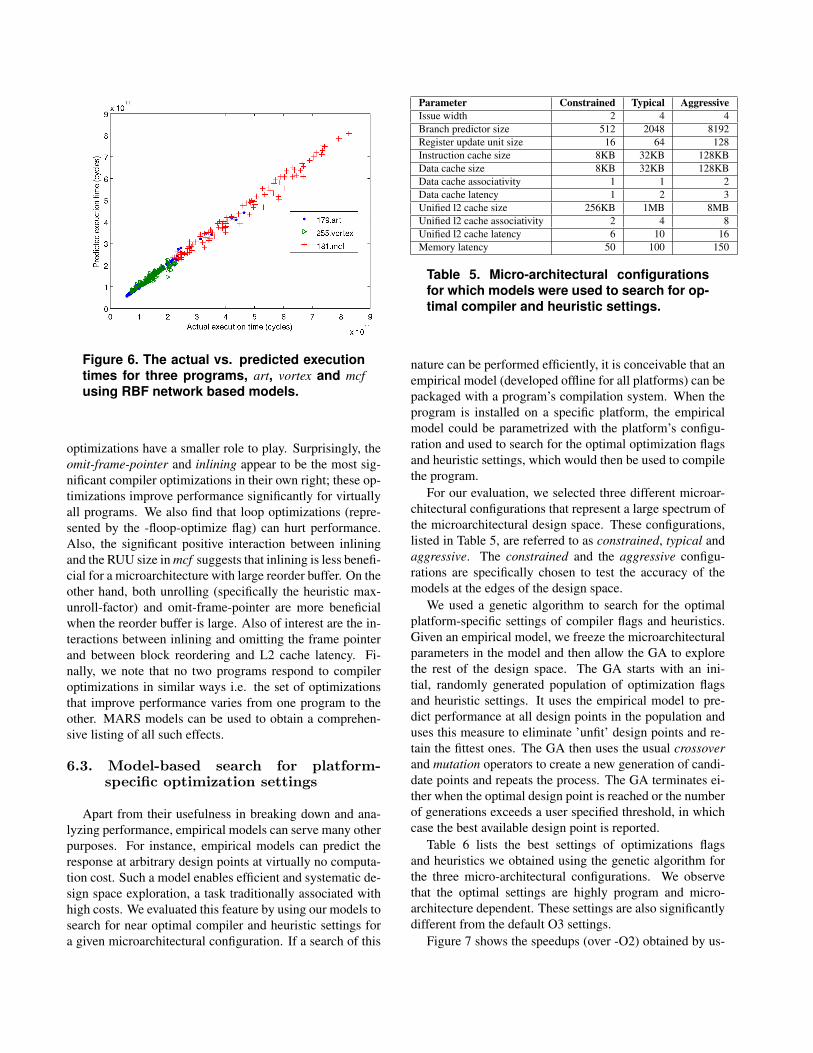
Figure 6. The actual vs. predicted executiontimes for three programs, art, vortex and mcfusing RBF network based models.

optimizations have a smaller role to play. Surprisingly, theomit-frame-pointer and inlining appear to be the most sig-nificant compiler optimizations in their own right; these op-timizations improve performance significantly for virtuallyall programs. We also find that loop optimizations (repre-sented by the -floop-optimize flag) can hurt performance.Also, the significant positive interaction between inliningand the RUU size in mcf suggests that inlining is less benefi-cial for a microarchitecture with large reorder buffer. On theother hand, both unrolling (specifically the heuristic max-unroll-factor) and omit-frame-pointer are more beneficialwhen the reorder buffer is large. Also of interest are the in-teractions between inlining and omitting the frame pointerand between block reordering and L2 cache latency. Fi-nally, we note that no two programs respond to compileroptimizations in similar ways i.e. the set of optimizationsthat improve performance varies from one program to theother. MARS models can be used to obtain a comprehen-sive listing of all such effects.

6.3. Model-based search for platform-specific optimization settings

Apart from their usefulness in breaking down and ana-lyzing performance, empirical models can serve many otherpurposes. For instance, empirical models can predict theresponse at arbitrary design points at virtually no computa-tion cost. Such a model enables efficient and systematic de-sign space exploration, a task traditionally associated withhigh costs. We evaluated this feature by using our models tosearch for near optimal compiler and heuristic settings fora given microarchitectural configuration. If a search of this

Parameter Constrained Typical AggressiveIssue width 2 4 4Branch predictor size 512 2048 8192Register update unit size 16 64 128Instruction cache size 8KB 32KB 128KBData cache size 8KB 32KB 128KBData cache associativity 1 1 2Data cache latency 1 2 3Unified l2 cache size 256KB 1MB 8MBUnified l2 cache associativity 2 4 8Unified l2 cache latency 6 10 16Memory latency 50 100 150

Table 5. Micro-architectural configurationsfor which models were used to search for op-timal compiler and heuristic settings.

nature can be performed efficiently, it is conceivable that anempirical model (developed offline for all platforms) can bepackaged with a program’s compilation system. When theprogram is installed on a specific platform, the empiricalmodel could be parametrized with the platform’s configu-ration and used to search for the optimal optimization flagsand heuristic settings, which would then be used to compilethe program.

For our evaluation, we selected three different microar-chitectural configurations that represent a large spectrum ofthe microarchitectural design space. These configurations,listed in Table 5, are referred to as constrained, typical andaggressive. The constrained and the aggressive configu-rations are specifically chosen to test the accuracy of themodels at the edges of the design space.

We used a genetic algorithm to search for the optimalplatform-specific settings of compiler flags and heuristics.Given an empirical model, we freeze the microarchitecturalparameters in the model and then allow the GA to explorethe rest of the design space. The GA starts with an ini-tial, randomly generated population of optimization flagsand heuristic settings. It uses the empirical model to pre-dict performance at all design points in the population anduses this measure to eliminate ’unfit’ design points and re-tain the fittest ones. The GA then uses the usual crossoverand mutation operators to create a new generation of candi-date points and repeats the process. The GA terminates ei-ther when the optimal design point is reached or the numberof generations exceeds a user specified threshold, in whichcase the best available design point is reported.

Table 6 lists the best settings of optimizations flagsand heuristics we obtained using the genetic algorithm forthe three micro-architectural configurations. We observethat the optimal settings are highly program and micro-architecture dependent. These settings are also significantlydifferent from the default O3 settings.

Figure 7 shows the speedups (over -O2) obtained by us-

Parameter/interaction 181.mcf 256.bzip2 175.vpr 255.vortex 164.gzip 179.art 177.mesaconstant (β0) 439.30 132.84 177.28 142.85 75.52 123.40 226.72issue width 0.00 -18.77 -7.27 -17.79 -11.73 0.00 -39.06RUU Size 0.00 -11.05 -39.56 -16.69 -4.25 -48.03 -25.56ul2 latency 5.54 1.91 2.90 15.32 3.40 0.00 29.33dl1 size 0.00 -1.94 -4.09 -4.61 -2.55 0.00 -6.69dl1 latency 0.00 2.77 2.63 3.44 1.98 0.00 0.00dl1 assoc 0.00 0.48 -1.43 -3.07 -1.18 0.00 0.00il1 size 0.00 -1.82 0.00 -24.17 -1.75 0.00 -50.22ul2 size -155.91 -12.92 -12.93 -9.74 0.00 -88.99 -5.19ul2 assoc 8.51 0.87 -2.67 -4.23 0.00 0.00 0.00memory latency 81.46 7.66 10.95 0.00 0.99 37.95 71.78issue width * RUU size 0.00 -1.97 -1.93 0.00 -2.42 0.00 0.00RUU Size * dl1 latency 0.00 -1.82 -1.59 -5.10 -1.83 0.00 0.00RUU Size * ul2 size 0.00 3.08 7.29 0.00 0.00 42.42 0.00RUU Size * memory latency 0.00 0.00 -4.23 0.00 0.00 -20.02 0.00il1 size * ul2 latency 0.00 0.00 0.00 -14.74 -1.31 0.00 -33.38ul2 size * memory latency -79.05 -6.55 -6.44 4.25 0.00 -42.13 0.00ul2 size * ul2 assoc -8.60 1.25 1.83 7.25 0.00 0.00 0.00ul2 assoc * memory latency 8.18 0.00 -1.77 0.00 0.00 0.00 0.00inlining -16.62 -0.90 -3.28 -2.17 -0.53 0.00 -5.81unrolling 0.00 -0.86 0.00 0.00 -0.93 0.00 0.00loop optimize 0.00 0.00 0.00 0.00 0.56 0.00 4.47reorder blocks 0.00 -0.73 0.00 0.00 0.00 0.00 -3.84gcse 0.00 0.00 0.00 -1.92 0.00 0.00 0.00omit frame pointer -7.82 -2.01 -2.23 -4.41 -1.27 0.00 -5.60max-inline-insns 0.00 0.00 -2.13 0.00 1.18 0.00 0.00max-unroll-factor 0.00 0.00 0.00 0.00 0.00 0.00 5.04inlining * RUU Size 10.33 0.00 0.00 0.00 0.00 0.00 0.00inlining * omit frame pointer 6.29 0.00 0.00 0.00 0.00 0.00 0.00inlining * ul2 latency 2.17 0.00 0.00 0.00 0.00 0.00 0.00omit frame pointer * issue width 0.00 0.76 0.00 0.00 0.69 0.00 0.00scheduling * il1 size 0.00 -0.71 0.00 0.00 0.00 0.00 0.00omit frame pointer * RUU Size 0.00 0.00 1.48 0.00 0.00 0.00 -8.20reorder blocks * ul2 latency 0.00 0.00 0.00 0.00 0.00 0.00 -6.32max-unroll-factor * RUU Size 0.00 0.00 0.00 0.00 0.00 0.00 -8.33

Table 4. Coefficients of key parameters and interactions inferred from the MARS models. The coeffi-cients represent execution time in billion of cycles.

Program-Input 1 2 3 4 5 6 7 8 9 10 11 12 13 14gzip-graphic 1/1/1 1/1/1 0/0/0 0/0/0 0/1/0 0/0/1 1/1/1 1/1/1 1/0/0 134/128/126 25/43/36 15/16/16 10/09/09 200/200/200vpr-route 1/1/1 1/0/0 0/0/0 1/0/1 0/0/0 0/0/0 1/1/1 1/1/1 1/1/1 138/141/137 48/47/47 12/12/19 11/04/12 300/300/300mesa-ref 1/1/1 0/0/1 1/0/0 0/0/0 1/0/1 1/1/0 1/1/1 1/1/1 0/0/1 108/108/105 75/75/55 16/16/16 08/08/08 151/152/166art-ref 1/0/0 1/1/1 1/1/0 1/1/1 1/1/1 1/1/1 0/0/0 0/0/1 1/1/1 100/050/050 55/75/75 16/12/20 08/12/04 206/300/300mcf-ref 1/1/1 1/1/1 1/1/1 0/0/1 0/1/1 1/1/1 1/1/1 0/0/1 0/0/1 080/050/050 50/50/75 16/16/12 08/08/12 200/200/100vortex-lendian1 1/1/1 1/0/0 0/0/0 0/0/0 1/1/1 1/1/1 1/1/1 1/1/0 1/0/0 100/100/100 25/25/25 18/18/18 10/10/09 200/200/200bzip2-graphic 1/1/1 1/1/1 0/0/0 0/0/1 0/0/0 0/0/1 1/1/1 1/1/1 0/0/0 100/100/100 58/62/60 16/16/16 10/12/09 300/299/216default O3 1/1/1 0/0/0 1/1/1 1/1/1 1/1/1 1/1/1 1/1/1 1/1/1 1/1/1 100/100/100 50/50/50 16/16/16 08/08/08 200/200/200

Table 6. Optimization flag and heuristic settings prescribed by model-based search using RBF mod-els for the conservative/typical/aggressive micro-architectural configurations.

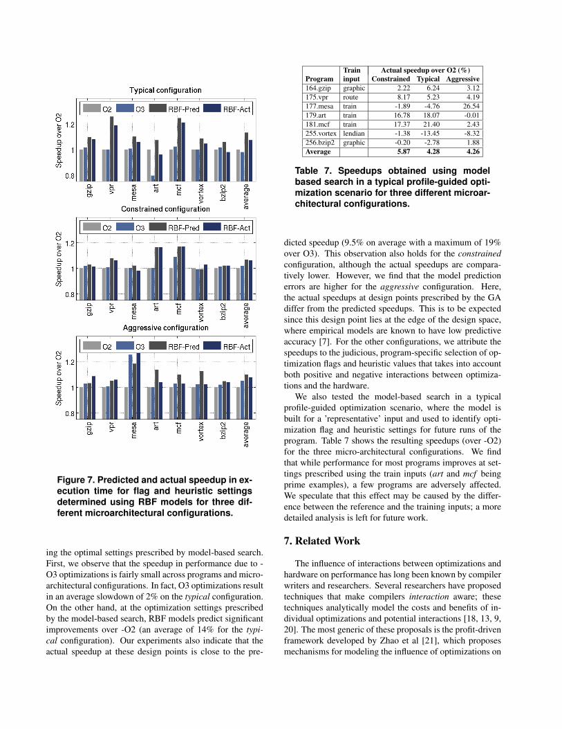
Figure 7. Predicted and actual speedup in ex-ecution time for flag and heuristic settingsdetermined using RBF models for three dif-ferent microarchitectural configurations.

ing the optimal settings prescribed by model-based search.First, we observe that the speedup in performance due to -O3 optimizations is fairly small across programs and micro-architectural configurations. In fact, O3 optimizations resultin an average slowdown of 2% on the typical configuration.On the other hand, at the optimization settings prescribedby the model-based search, RBF models predict significantimprovements over -O2 (an average of 14% for the typi-cal configuration). Our experiments also indicate that theactual speedup at these design points is close to the pre-

Train Actual speedup over O2 (%)Program input Constrained Typical Aggressive164.gzip graphic 2.22 6.24 3.12175.vpr route 8.17 5.23 4.19177.mesa train -1.89 -4.76 26.54179.art train 16.78 18.07 -0.01181.mcf train 17.37 21.40 2.43255.vortex lendian -1.38 -13.45 -8.32256.bzip2 graphic -0.20 -2.78 1.88Average 5.87 4.28 4.26

Table 7. Speedups obtained using modelbased search in a typical profile-guided opti-mization scenario for three different microar-chitectural configurations.

dicted speedup (9.5% on average with a maximum of 19%over O3). This observation also holds for the constrainedconfiguration, although the actual speedups are compara-tively lower. However, we find that the model predictionerrors are higher for the aggressive configuration. Here,the actual speedups at design points prescribed by the GAdiffer from the predicted speedups. This is to be expectedsince this design point lies at the edge of the design space,where empirical models are known to have low predictiveaccuracy [7]. For the other configurations, we attribute thespeedups to the judicious, program-specific selection of op-timization flags and heuristic values that takes into accountboth positive and negative interactions between optimiza-tions and the hardware.

We also tested the model-based search in a typicalprofile-guided optimization scenario, where the model isbuilt for a ’representative’ input and used to identify opti-mization flag and heuristic settings for future runs of theprogram. Table 7 shows the resulting speedups (over -O2)for the three micro-architectural configurations. We findthat while performance for most programs improves at set-tings prescribed using the train inputs (art and mcf beingprime examples), a few programs are adversely affected.We speculate that this effect may be caused by the differ-ence between the reference and the training inputs; a moredetailed analysis is left for future work.

7. Related Work

The influence of interactions between optimizations andhardware on performance has long been known by compilerwriters and researchers. Several researchers have proposedtechniques that make compilers interaction aware; thesetechniques analytically model the costs and benefits of in-dividual optimizations and potential interactions [18, 13, 9,20]. The most generic of these proposals is the profit-drivenframework developed by Zhao et al [21], which proposesmechanisms for modeling the influence of optimizations on

code and machine resources. These methods typically an-alyze optimization sites in isolation and make several sim-plifying assumptions such as the additive nature of costsand benefits and the lack of interactions between optimiza-tions and hardware components such as the reorder bufferor branch predictors.

Several researchers have recognized the inherent com-plexity of understanding and modeling interactions betweenoptimizations and opted for the use of statistical and ma-chine learning techniques to address these problems instead.Haneda et al [6] propose the use of statistical inference tech-niques for selection of optimal optimization flags on a givenplatform. Search and learning techniques have been used toto identify efficient compilation sequences [17, 2, 10, 1].and to improve optimization specific heuristics [15]. Manyof these techniques are based on the key idea that the ef-fect of compiler optimizations on a program is related tocertain key program features. Cazavos et al [4] propose theuse of neural networks and reaction-based modeling tech-niques to build empirical models for compiler optimiza-tions. Their modeling technique is based on the assumptionthat a program can be characterized by the way it respondsto a set of characteristic optimizations. In contrast to theseapproaches, our models are platform independent but spe-cific to each program-input pair. Our models are designedto generalize across a complex and important but often ig-nored micro-architectural design space.

8. Conclusions

In this paper, we proposed the use of empirical mod-eling techniques to build application-specific performancemodels for compiler optimizations. The key feature of ourmodeling process is the ability to simultaneously capturethe effects and interactions between several compiler opti-mizations, associated heuristics and microarchitectural pa-rameters without any prior knowledge about their behavior.We show that empirical models can be effective tools in thehands of compiler writers. The models assist a compilerwriter in identifying key effects and interactions that have ahigh impact on performance, and thus provide informationuseful for designing better analytical models and optimiza-tion heuristics. The models also enable efficient searchesover parts of the design space, as illustrated by our use ofthe models for searching optimal compiler flags and heuris-tics for any arbitrary hardware platform.

References

[1] F. Agakov, E. Bonilla, J. Cavazos, B. Franke, G. Fursin,M. F. P. Boyle, J. Thomson, M. Toussaint, and C. K. I.Williams. Using Machine Learning to Focus Iterative Op-timization. In Proc. of CGO, 2006.

[2] L. Almagor, K. Cooper, A. Grosul, T. Harvey, S. Reeves,D. Subramaniam, L. Torczon, and T. Waterman. FindingEffective Compilation Sequences. In Proc. of LCTES, 2004.

[3] D. S. Broomhead and D. Love. Multivariate Function Inter-polation and Adaptive Networks. Complex Systems, 1988.

[4] J. Cavazos, C. Dubach, F. Agakov, E. Bonilla, M. F. P.O’Boyle, G. Fursin, and O. Temam. Automatic PerformanceModel Construction for the Fast Software Exploration ofNew Hardware Designs. In Proc. of CASES, 2006.

[5] J. H. Friedman. Multivariate Adaptive Regression Splines.The Annals of Statistics, pages 1–141, 1991.

[6] M. Haneda, P. M. W. Knijnenburg, and H. A. G. Wi-jshoff. Automatic Selection of Compiler Options using Non-parametric Inferential Statistics. In Proc. of PACT, 2005.

[7] P. J. Joseph, K. Vaswani, and M. J. Thazhuthaveetil. A Pre-dictive Model for Superscalar Processor Performance. InProc. of MICRO, 2006.

[8] P. J. Joseph, K. Vaswani, and M. J. Thazhuthaveetil. Con-struction and Use of Linear Regression Models for Proces-sor Performance Analysis. In Proc. of HPCA, 2006.

[9] T. Kisuki, P. M. W. KnijnenBurg, and M. F. P. O’Boyle.Combined Selection of Tile Size and Unroll Factors usingIterative Compilation. In Proc. of PACT, 2000.

[10] P. Kulkarni, S. Hines, J. Hiser, D. Whalley, J. Davidson, andD. Jones. Fast Searches for Effective Optimization PhaseSequences. In Proc. of PLDI, 2004.

[11] D. C. Montgomery. Design and Analysis of Experiments.Wiley, 5th edition, 2001.

[12] M. Orr, J. Hallam, K. Takezawa, A. Murray, S. Ninomiya,M. Oide, and T. Leonard. Combining Regression Trees andRadial Basis Function Networks. International Journal ofNeural Systems, 2000.

[13] V. Sarkar and N. Megiddo. An Analytic Model for LoopTiling and its Solution. In Proc. of ISPASS, 2000.

[14] T. Sherwood, E. Perelman, G. Hamerly, and B. Calder. Au-tomatically Characterizing Large Scale Program Behavior.In Proc. of ASPLOS, 2002.

[15] M. Stephenson and S. Amarasinghe. Predicting Unroll Fac-tors Using Supervised Classification. In Proc. of CGO,2005.

[16] M. Stephenson, S. Amarasinghe, M. Martin, and U.-M. O-Reily. Meta Optimization: Improving Compiler Heuristicsusing Machine Learning. In Proc. of PLDI, 2003.

[17] S. Triantafyllis, M. Vachharajani, N. Vachharajani, and D. I.August. Compiler Optimization Space Exploration. In Proc.of CGO, 2003.

[18] M. E. Wolf, D. E. Maydan, and D. Chen. Combining LoopTransformations Considering Caches and Scheduling. InProc. of MICRO, 1996.

[19] R. E. Wunderlich, B. F. T. F. Wenisch, and J. C. Hoe.SMARTS: Accelerating Microarchitecture Simulation viaRigorous Statistical Sampling. In Proc. of ISCA, 2003.

[20] M. Zhao, B. R. Childers, and M. L. Soffa. Predicting theImpact of Optimizations for Embedded Systems. In Proc. ofLCTES, 2003.

[21] M. Zhao, B. R. Childers, and M. L. Soffa. A Model-basedFramework: an Approach to Profit-driven Optimization. InProc. of CGO, 2005.