Sensors 2007, 7, 1069-1090

sensorsISSN 1424-8220c© 2007 by MDPI

www.mdpi.org/sensors

Full Paper

Methods for Solving Gas Damping Problems in PerforatedMicrostructures Using a 2D Finite-Element Solver

Timo Veijola 1,� and Peter Raback 2

1 Helsinki University of Technology, P.O. Box 3000, FIN-02015 TKK, Finland, E-mail:

timo.veijola@tkk.fi2 CSC – Scientific Computing Ltd., P.O. Box 405, FIN-02101 Espoo, Finland. E-mail: raback@csc.fi� Author to whom correspondence should be addressed.

Received: 18 May 2007 / Accepted: 27 June 2007 / Published: 28 June 2007

Abstract: We present a straightforward method to solve gas damping problems for perfo-

rated structures in two dimensions (2D) utilising a Perforation Profile Reynolds (PPR) solver.

The PPR equation is an extended Reynolds equation that includes additional terms modelling

the leakage flow through the perforations, and variable diffusivity and compressibility pro-

files. The solution method consists of two phases: 1) determination of the specific admittance

profile and relative diffusivity (and relative compressibility) profiles due to the perforation,

and 2) solution of the PPR equation with a FEM solver in 2D. Rarefied gas corrections in

the slip-flow region are also included. Analytic profiles for circular and square holes with

slip conditions are presented in the paper. To verify the method, square perforated dampers

with 16 – 64 holes were simulated with a three-dimensional (3D) Navier-Stokes solver, a ho-

mogenised extended Reynolds solver, and a 2D PPR solver. Cases for both translational (in

normal to the surfaces) and torsional motion were simulated. The presented method extends

the region of accurate simulation of perforated structures to cases where the homogenisation

method is inaccurate and the full 3D Navier-Stokes simulation is too time-consuming.

Keywords: damping, perforation, gas damper, rarefied gas, Reynolds equation

1. Introduction

Perforations are used in oscillating microelectromechanical (MEM) sensors and actuators to control

damping due to gas for desired frequency-domain operation. Practical MEM devices using perforations

Sensors 2007, 7 1070

include microphones [1], capacitive switches [2, 3], and resonators [4].

The perforations reduce damping in a squeeze-film structure considerably: the characteristic dimen-

sions are reduced from the outer dimensions of the surface to the separation of the perforations. Also, the

cut-off frequency (when the spring and damping forces are equal) rises considerably due to the perfora-

tions. Often this cut-off frequency in perforated structures is much higher than the operating frequencies

of interest, which simplifies the design of such devices since only the damping forces need to be consid-

ered in the device design.

3D flow simulations are needed in solving perforation problems generally. However, accurate 3D

simulation of the Navier-Stokes (N-S) equation is, in practice, impossible due to the huge number of

elements needed, especially in cases where the number of perforations is relatively large. The number of

perforations may vary from a few holes to a grid of thousands of holes. Moreover, the N-S equations are

limited to the region of a slightly rarefied gas (slip-flow region). Accurate modelling of these structures

requires the consideration of rarefied gas flow in tiny flow channels and around the structure.

Different methods that reduce the 3D flow problem into 2D are available, depending on the boundary

conditions, number of perforations, the relative hole size s0/h (s0 is the hole diameter and h is the

height of the air gap) and the perforation ratio (ratio of the perforated area and the surface area). If

the s0/h-ratio is large, the flow resistance of the perforation is insignificant (unless the perforations

are relatively long). In the case of a few relatively large perforations, the problem reduces to a 2D

problem that can be solved from the Reynolds equation by considering the holes as additional boundary

conditions [5, 6]. Open edge corrections [7] might need to be considered in this case. On the other hand,

if the number of holes is large, and the perforation ratio is not small, the horizontal flow from the damper

borders is insignificant (also caused by closed damper borders), and the pressure patterns around each

perforation are identical. In this case, the damping can be determined solely from a single perforation

and its surroundings, called a perforation cell. A simple analytic model for such a cell by Skvor [8]

has been used in modelling perforations in a microphone’s backplate. When the s0/h-ratio cannot be

considered large, the flow resistance of the perforations must be included in the model. Homentcovschi

and Miles [9], have derived such an analytic model considering the compressibility and inertial effects.

Perforation cell models over a wide range of perforation ratios and hole lengths well below the cut-off

frequency are given in [10, 11].

If the s0/h ratio and the perforation ratio are not large, such that the flow from the damper borders

is considerable, a more complicated model is required. In the case of a regular grid of perforations, the

flow resistance of the perforation cell can be solved and homogenised over the damper surface. This

flow problem can be modelled with the extended Reynolds equation that contains an additional pressure

leakage term [12–16]. This homogenisation method is usable, but it has its limitations, especially if the

number of perforations is small. A mixed-level approach has also been published [17], and a hybrid

method combining N-S and Reynolds equations has been presented by da Silva et al. [18]. Flow resis-

tances of perforations with different shapes were studied by Homentcovschi and Miles [19]. A compact

analytic model for rectangular dampers having an uniform perforation was given in [10]. The model

was verified with FEM simulations at frequencies well below the cut-off frequency.

The models referenced above assume motion normal to the surfaces, and the squeezing force in the

Sensors 2007, 7 1071

air gap makes the gas flow. A different problem where the perforated surface moves tangentially to the

surfaces has been discussed in [20].

We have presented a Perforation Profile Reynolds (PPR) method [21] for damping problems where

the homogenisation method is not accurate. These are characterized by, e.g., a moderate number of

perforations, complex shaped perforations, and non-uniform distribution and sizes of perforations.

In this paper, we present improvements to this method. Flow admittance profiles that vary across the

perforations are used instead of constant profiles. Also, an improved perforation cell model [10] has

been used instead of a simple theoretical long-channel model with theoretical end corrections. Besides

translational motion, the verifications include also torsional motion. This paper also shows how the

perforation cell model [10] can be utilised in a homogenisation method with a FEM solver.

The method was verified with 3D FEM simulations using a N-S solver. Simulations of a parallel-

plate damper with 16 to 64 square perforations were performed for various perforation ratios. Only

incompressible flow is considered here, since time-harmonic reference N-S simulation with sufficient

accuracy is not realistic.

2. Methods

2.1. PPR equation

Figure 1 shows the general geometry of a perforated gas damper. A perforated surface above the

ground surface moves normal to the surfaces (in the direction of the z-axis).

x

zy

u

h

v

u

Figure 1. General geometry of a perforated gas damper.

Gas lubrication and damping problems in small air gaps are traditionally modelled with the Reynolds

equation [22]. The modified and linearised Reynolds equation in the time-harmonic form is

∇ ·

(h3Qch

12η∇p

)−jωhp

PA= vz, (1)

where h is the static air gap height, η is the viscosity coefficient, Qch is the relative flow rate, PA is the

ambient pressure, vz(x, y)ejωt is the surface velocity in the z-direction and p(x, y)ejωt is the pressure

variation to be solved from the equation. This form allows the static displacement h(x, y) to be a func-

tion of x and y. In this case, the spatial dependency of Qch(x, y) must be considered, too. Isothermal

conditions have been assumed.

Sensors 2007, 7 1072

We extend the Reynolds equation by adding a term that models an additional flow component through

the perforations similarly as in [12]. Here, two additional coefficients are included to model the effect of

the perforations on the diffusivity and compressibility.

∇ ·

(Dhh3Qch

12η∇p

)− Ch

jωhp

PA− Yhp = vz, (2)

where Dh(x, y), Ch(x, y), and Yh(x, y) are the relative diffusivity, relative compressibility, and perfora-

tion admittance profiles, respectively. Equation (2) is called here the Perforation Profile Reynolds (PPR)

equation.

The perforation admittance Yh is specified as an inverse of the specific acoustic impedance ZS:

Yh =1

ZS=vh

ph, (3)

where ph and vh are the gas pressure and velocity in the z-direction at the opening of the perforation.

Equation (3) is valid also for the quantities averaged across the cross-section of the perforation, denoted

as Y h, ZS, vh, and ph.

The approximation for the relative flow rate due to the rarefied gas effects is [23]

Qch = 1 + 9.638K1.159n,ch , (4)

whereKn,ch = λ/h is the Knudsen number of the air gap and λ is the mean free path of the gas (depends

on PA). The relative accuracy is valid for Kn,ch < 880 and its maximum relative error is less than 5%.

When the slip correction is considered, as in this paper,

Qch = 1 + 6Kn,ch. (5)

The slip correction is valid only for Kn,ch < 0.1, whereas the approximation in Eq.( 4) is valid for much

larger Knudsen numbers. The slip correction is used in this paper, since for us the validation with a 3D

FEM solver is only possible in the slip-flow region.

2.2. PPR method

The PPR method consists of two phases. First, diffusivity, compressibility, and perforation admit-

tance profiles in Eq. (2) are determined. Then, the PPR solver is used to solve Eq. (2). In PPR, the

specific admittance profile Yh(x, y) varies spatially at the locations of the perforations, whereas in the

homogenisation method Yh includes the flow resistance of the perforation cell, that is, the flow in the air

gap and the perforations.

In [21], we used a constant average admittance profile for each perforation. This admittance was

calculated from the flow resistance of the perforation. In this work, we consider a varying admittance

profile across the perforation utilising the velocity profile in the perforation:

Yh(x, y) =

vh(x, y)

ph, inside the perforation

0 , outside,(6)

Sensors 2007, 7 1073

where vh is the velocity profile and ph is the pressure.

The diffusivity of the air gap also effectively changes at the perforation. For the flow passing in

the air gap below the perforation, the frictional surface area will be reduced, effectively increasing the

diffusivity coefficient. On the other hand, the flow profile is changed due to the perforations, effectively

decreasing the diffusivity coefficient Dh. The compressibility coefficient Ch is zero at the perforations

and unity elsewhere. Figure 2 illustrates the perforation profiles in the case of a one-dimensional damper.

Yh

a)

Dh

0

1

b)

Ch

0

1

Figure 2. a) Topology of a single perforation in 2D and b) reduced profiles in 1D for Eq. (2).

2.3. Perforation Admittance Profiles

There are two alternate ways to determine the flow admittance profiles for perforations: 3D FEM (or

other discretising methods) simulations and analytic (approximate) equations. Usually, the perforations

are relatively short and the analytic model for long channels are not applicable. Here, flow resistances

extracted from FEM simulations of the perforation cells are used [10, 11].

The flow fields above the perforated surface are coupled, especially when the perforation ratio is

large. In [10] an elongation model considering the coupling in circular perforations is derived from

FEM simulations. The model assumes that the conditions for neighbouring perforations are identical. In

principle, these conditions are met if the perforation ratio is large and the velocity distribution vz(x, y)

of the damper surface is constant. However, in practice the coupling is negligible for small perforation

ratios, and there are no abrupt changes in the damper surface velocity for neighbouring perforations.

Next, analytic expressions for two typical perforations, circular and square, are given (See Fig. 3).

Sensors 2007, 7 1074

s0

a) b)

r x

y

r0

Figure 3. Cross-sections and dimensions of a) circular and b) square perforations.

2.4. Circular Cross-section

For the flow resistance of the perforation we utilise the perforation cell model [10]. Here, the flow

resistances modelling the perforation only are needed, since the PPR solver calculates the flow in the air

gap. The (average) specific admittance of a channel (of length hc) with a circular cross-section (with a

radius of r0) in the slip-flow region is [10]

Y ci =πr20

RIC +RC +RE, (7)

where the flow resistances RIC, RC and RE are given in Appendix. RC is the mechanical resistance of

a long channel with a circular cross-section. In the slip-flow region, the relative flow rate of a channel

with a circular cross-section Qtb is

Qtb = 1 + 4Kn,tb, (8)

where Kn,tb is the Knudsen number of the capillary

Kn,tb = λ/r0. (9)

The normalised velocity profile (average velocity is 1) in a long circular capillary is a function of r

only [24]:

vs(r) = 2−(r

r0

)2+ 1 + 2Kn,tb

Qtb. (10)

The specific admittance profile resulting from Eqs. (7) and (10) is

Yci(r) = vs(r)Y ci. (11)

2.5. Square Cross-section

Mechanical flow resistance of a long square channel is [25, 26]

Rsq =28.454ηhc

Qsq, (12)

where Qsq is the flow rate coefficient and hc is the length of the channel. Next, the short-channel effects

are added toRsq using the elongation model for a circular channel [10]. In that model, an effective radius

Sensors 2007, 7 1075

r0 is needed. It is specified such that the acoustic resistances (hydraulic resistances) of the square and

circular long channels are equal. That is

RC

(πr20)2=Rsq

s40. (13)

This results in an expression for r0:

r0 =

(128Qsq

28.454πQtb

) 14 s0

2≈ 1.096 ·

s0

2. (14)

Since Qtb is a function of r0, the accurate solution of Eq. (14) needs to be iterated. The dependency of r0on the Knudsen number is small, and the simple approximation in Eq. (14) is accurate within 0.3% for

Kn,sl < 0.14.

2.6. Homogenisation method

In the homogenisation method, the flow admittane Yh caused by the perforations is assumed to be

smoothly distributed over the whole surface. In the actual 2D FEM simulation, the holes are excluded

from the simulated structure and their flow admittance is included in the extended Reynolds equation.

In the case of uniform perforation, this flow admittance is constant over the whole surface. Damping

models using the homogenization approach have been published, but not properly verified [12–16].

The PPR equation (2) is applicable also in the homogenisation method, but there is a considerable

difference in the interpretation of term Yh. In addition to the flow admittance of the perforations itself,

Yh should now include the flow component in the air gap.

In deriving the model for Yh, the concept of a “perforation cell” is applied here. Relative simple

analytic models for a cylindrical and square perforation is derived in [10] and [11], respectively, based

on compact models derived from FEM simulations. The mechanical resistance of each perforation cell

consists of mechanical resistances of several flow regions [10]:

Rp = RS +RIS +RIB +r4xr40(RIC +RC +RE) , (15)

where rx and r0 are the outer and inner radii of the cylindrical perforation cell, respectively. RS is the

flow resistance in the air gap andRC is the flow resistance of the perforation. All other resistances model

the flow in the intermediate region under and above the perforation. Values for these resistances are

given in Appendix.

Radius rx is selected such that the bottom areas of circular and square cells match. This results in

rx =sx√π. (16)

In the case of uniform perforation and translational motion, the specific impedance spread all over the

surface is

Yh =a2eff

NRp, (17)

where aeff = a+ 1.3h(1 + 3.3Kn,ch) is the effective dimension of the surface.

Sensors 2007, 7 1076

3. Verification

Several perforated dampers in perpendicular and rotating motion are simulated both with the 3D N-S

solver with slip conditions and with the time-harmonic PPR solver. Both solvers are implemented in the

multiphysical simulation software Elmer [27].

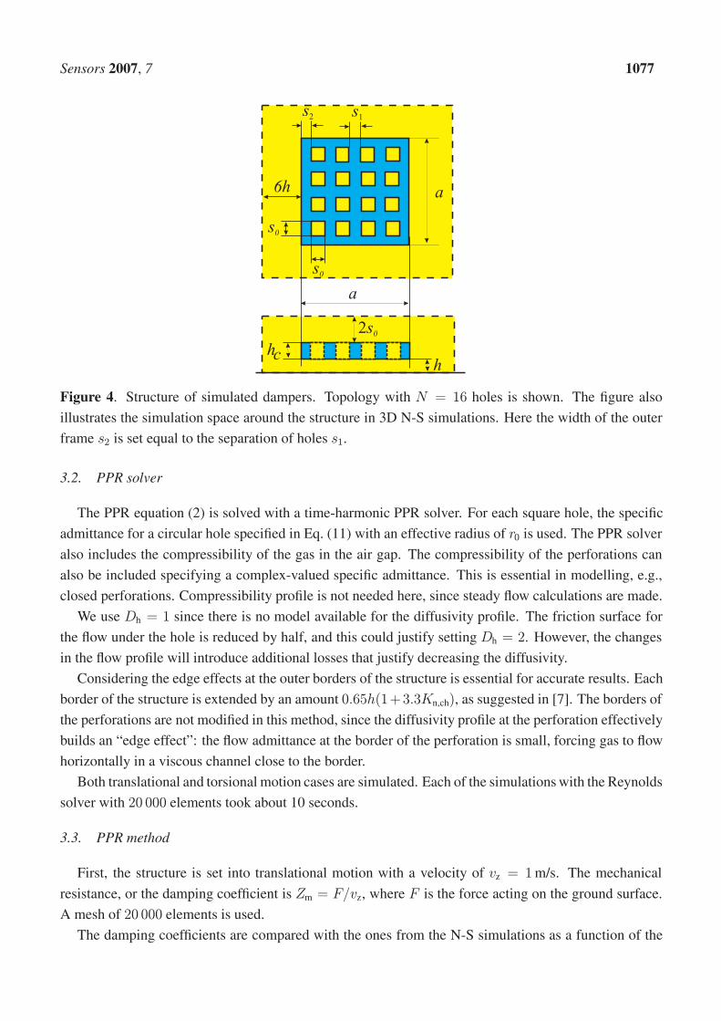
The surface is a square, and it consists of N square holes. The distance between the edges of two

adjacent holes is s1, as is the distance from the edges of the holes to the edges of the damper s2 = s1.

The perforation pitch is sx = s0+s1. A comparison is made well below the cut-off frequency, that is, the

compressibility of the gas is ignored (Ch = 0). The simplifies the N-S simulations, since response to a

constant velocity is calculated. The dimensions are summarised in Table 1 and one of the four structures

is shown in Fig. 4.

Table 1. Parameters for the simulated dampers. Altogether, 504 different topologies were generated and

simulated.

Description Values Unit

Number of holes N 16, 36, 64

Surface length a 20, 30, 40 10−6m

Hole diameter s0 0.5, 1.0, . . . , 4.5 10−6m

Thickness hc 0.5, 1, 2, 5 10−6m

Air gap height h 1, 2 10−6m

Viscosity coefficient η 20 10−6Ns/m2

Mean free path λ 69 10−9m

3.1. 3D simulations

First, full 3D N-S simulations of the structure are performed to generate reference data for the methods

presented in this paper. The simulations can be performed relatively reliably, thanks to the small number

of holes and the symmetry of the structure. Slip boundary conditions are used for the surfaces. The

simulated gas volume is extended around the damper: free space around and above the damper are 6h

and 2s0, respectively. A mesh of 450 000 elements is used. Both translational and torsional motion cases

were simulated.

The number of elements (450 000) in the 3D N-S simulations was in practice the maximum that could

be performed considering the computing time and the memory consumption. The computer used was

Sun Fire 25K. Simulating each (of 432) topology took between one and two hours and 6Gb of memory.

To estimate the accuracy of the results, simulations with 250 000 elements were made, too. Compar-

ative results are discussed later in this paper.

Sensors 2007, 7 1077

s0

a

2s0

6h a

s0

s2 s1

hh

c

Figure 4. Structure of simulated dampers. Topology with N = 16 holes is shown. The figure also

illustrates the simulation space around the structure in 3D N-S simulations. Here the width of the outer

frame s2 is set equal to the separation of holes s1.

3.2. PPR solver

The PPR equation (2) is solved with a time-harmonic PPR solver. For each square hole, the specific

admittance for a circular hole specified in Eq. (11) with an effective radius of r0 is used. The PPR solver

also includes the compressibility of the gas in the air gap. The compressibility of the perforations can

also be included specifying a complex-valued specific admittance. This is essential in modelling, e.g.,

closed perforations. Compressibility profile is not needed here, since steady flow calculations are made.

We use Dh = 1 since there is no model available for the diffusivity profile. The friction surface for

the flow under the hole is reduced by half, and this could justify setting Dh = 2. However, the changes

in the flow profile will introduce additional losses that justify decreasing the diffusivity.

Considering the edge effects at the outer borders of the structure is essential for accurate results. Each

border of the structure is extended by an amount 0.65h(1+3.3Kn,ch), as suggested in [7]. The borders of

the perforations are not modified in this method, since the diffusivity profile at the perforation effectively

builds an “edge effect”: the flow admittance at the border of the perforation is small, forcing gas to flow

horizontally in a viscous channel close to the border.

Both translational and torsional motion cases are simulated. Each of the simulations with the Reynolds

solver with 20 000 elements took about 10 seconds.

3.3. PPR method

First, the structure is set into translational motion with a velocity of vz = 1m/s. The mechanical

resistance, or the damping coefficient is Zm = F/vz, where F is the force acting on the ground surface.

A mesh of 20 000 elements is used.

The damping coefficients are compared with the ones from the N-S simulations as a function of the

Sensors 2007, 7 1078

perforation ratio

q =Ns20a2· 100% (18)

The maximum relative errors in the damping coefficient are shown in Table 2, and Fig. 5 shows the

damping coefficients as a function of the perforation ratio q for air gaps of 1µm and 2µm. In Fig. 6, the

simulated pressure profiles are compared.

Table 2. Maximum relative errors in the translational motion damping coefficient Zm simulated with the

PPR method. Each row includes cases for d = 1µm or 2µm and hc = 0.5µm . . . 5µm. Comparison is

made against the 3D simulations with the N-S solver.

Max. relative error [%]s0 q

µm % N=16 N=36 N=64

0.5 1 -4.8 -2.3 -1.4

1.0 4 -4.9 -2.3 -3.4

1.5 9 -4.8 -2.3 -1.8

2.0 16 -4.8 -2.8 -3.4

2.5 25 -5.7 -4.9 -5.0

3.0 36 -8.3 -7.7 -7.7

3.5 49 -11.6 -11.2 -10.9

4.0 64 -15.6 -15.1 -15.1

4.5 81 -19.8 -19.3 -19.3

Next, the structure is set into torsional motion about the y-axis with a velocity of vz = 1m/s at

x = a/2. The torsional resistance, or the torsional damping coefficient is Zt = τ/ωz, where τ is the

twisting moment acting on the ground surface and ωz = vz/(a/2) is angular velocity. A mesh of 20 000

elements is used. The maximum relative errors in the torsional motion are shown in Table 3.

Figure 7 shows the torsional damping coefficients as a function of the perforation ratio for air gaps of

1µm and 2µm.

3.4. Homogenisation method

The extended Reynolds equation is solved for perpendicularly moving rectangular surfaces. The per-

foration cell admittance calculated from Eq. (17) is used in the simulation. The diffusivity coefficient

Dh = 1 is used. Each damper border is extended by 0.65h(1 + 3.3Kn,ch). The quarter of the rect-

angular surface is meshed having 5 000 elements. Table 4 shows the maximum relative errors of the

homogenisation method.

Sensors 2007, 7 1079

0 25 50 75 10030n

100n

300n

1µ

3µ

10µ

APLAC 8.30 User: HUT Circuit Theory Lab. Wed Jun 27 2007

Zm

q/%

N = 64N = 36

N = 16

a)

0 25 50 75 100

30n

100n

300n

1µ

3µAPLAC 8.30 User: HUT Circuit Theory Lab. Wed Jun 27 2007

Zm

q/%

N = 64

N = 36

N = 16

b)

Figure 5. Damping coefficients of the perforated dampers in translational motion simulated with the full

3D N-S solver (�) and with the PPR solver (——) as a function of the perforation ratio. N is 16, 36,

and 64, and the damper height hc is 0.5µm, 1µm, 2µm, and 5µm. The air gap height is a) 1µm and b)

2µm.

Sensors 2007, 7 1080

a)

b)

c)

d)

Figure 6. Pressure profiles on the bottom surface simulated with the full 3D N-S solver (left) and with

the PPR solver (right) for translational movement. The hole diameters are: a) 1µm, b) 2µm c) 3µm,

and d) 4µm. The number of perforationsN = 64, the air gap height is h = 1µm, and the surface height

hc = 1µm. Simulated quarters of bottom surfaces are shown.

Sensors 2007, 7 1081

0 25 50 75 1001a

3a

10a

30a

100a

300a

APLAC 7.92 User: HUT Circuit Theory Lab. Thu Jun 22 2006

Zt

q/%

N=64

N=36

N=16

a)

0 25 50 75 100

1a

3a

10a

30a

100a

APLAC 7.92 User: HUT Circuit Theory Lab. Thu Jun 22 2006

Zt

q/%

N=36

N=16

N=64

b)

Figure 7. Damping coefficients of the perforated dampers in torsional motion simulated with the full 3D

N-S solver (�) and with the PPR solver (——) as a function of the perforation ratio. N is 16, 36, and 64,

and the damper height hc is 0.5µm, 1µm, 2µm, and 5µm. The air gap height is a) 1µm and b) 2µm.

Sensors 2007, 7 1082

Table 3. Maximum relative errors in the torsional motion damping coefficient Zt simulated with the PPR

method. Each row includes cases for d = 1µm or 2µm and hc = 0.5µm . . . 5µm. Comparison is made

against the 3D simulations with the N-S solver.

Max. relative error [%]s0 q

µm % N=16 N=36 N=64

0.5 1 -18.0 -8.0 -4.4

1.0 4 -18.4 -8.3 -4.6

1.5 9 -18.7 -8.4 -4.6

2.0 16 -19.0 -8.5 -4.8

2.5 25 -19.6 -8.8 -7.2

3.0 36 -20.4 -11.3 -9.7

3.5 49 -21.9 -15.1 -13.7

4.0 64 -24.3 -19.5 -18.0

4.5 81 -28.5 -24.3 -22.9

4. Discussion

4.1. Comparison between methods

Table 2 shows the errors of the PPR method compared with the 3D FEM simulations for translational

motion. The maximum relative error in the damping force in translational motion is below 10%, except

for the case of strong perforation (q ≥ 49%). The PPR model generally underestimates the damping.

This is probably due to the fact that additional drag forces acting on the sidewalls and on the top surface

are ignored in the model. These forces contribute most when the surface is the thickest (hc = 5µm) and

the surface area is the smallest (N = 16).

In the case of torsional motion, Table 3, the accuracy of the model is approximately the same as for

translational motion forN = 64. The contribution of the drag forces can be seen in the results of smaller

surfaces in Fig. 7. In the torsional motion the drag forces acting on the sidewalls are relatively stronger.

For small q, the change in the height of the surface changes the damping force for N = 16 in the N-S

simulations, see Fig. 7b). The surface height clearly changes the damping coefficient (N-S simulations)

even for very small perforation ratios. This change cannot be explained by the change in the perforation

length, since the damping due to perforations is negligible for very small perforation ratios.

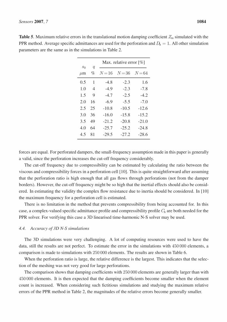
To analyse the importance of the varying pressure profile at the perforations, a set of PPR simulations

was performed using a constant specific admittance Y ci of the perforations. The results are summarised

in Table 5. Comparison with results in Table 2 reveals that errors of both models are approximately the

same for small perforation ratios, but the error of the constant specific admittance model is considerably

larger if q > 16%.

The maximum relative errors of the homogenisation method (Table 4) are also approximately below

Sensors 2007, 7 1083

Table 4. Maximum relative errors in the translational motion damping coefficient Zm simulated with

the homogenisation method. Each row includes cases for d = 1µm or 2µm and hc = 0.5µm . . . 5µm.

Comparison is made against the 3D simulations with the N-S solver.

Max. relative error [%]s0 q

µm % N=16 N=36 N=64

0.5 1 -4.9 -2.3 1.9

1.0 4 -5.0 6.4 6.0

1.5 9 8.8 10.6 9.7

2.0 16 9.4 9.6 8.7

2.5 25 7.6 7.5 6.6

3.0 36 -8.2 5.2 5.0

3.5 49 -11.3 -6.6 -4.3

4.0 64 -15.1 -9.4 -6.6

4.5 81 -19.6 -13.0 -9.3

10% for N ≥ 16 and q < 49%, but the PPR results are much better for small perforation ratios.

However, the homogenisation method gives better results when N ≥ 16 for q ≥ 50%. This was an

expected result. For an inhomogeneous perforation, where the distribution and sizes of the perforations

vary, the determination of the perforation cell might be difficult. In such a case, the generation of

the variable perforation admittance profile is not a trivial task. On the other hand, if the number of

perforations is large (hundreds or thousands of holes) the element sizes in the PPR method will grow

intolerably. In this case, the homogenisation method is superior since the required element count is

independent of the number of perforations.

4.2. Rarefied gas effects

The verification in this paper is limited to the slip-flow region just to make the comparison with 3D

solutions possible. The PPR method itself is valid for arbitrary gas rarefaction as long as the model for Yh

is valid. The comparison is made in the region where the validity of the slip conditions is questionable

(Kn,sl < 0.14, Kn,ch < 0.14). In spite of the small additional error in the results, the comparison is

justified since slip flow models are used in both cases. The consideration of the slip correction is essential

for accurate results for the micromechanical structures simulated. If the rarefied gas effects are ignored

(Kn,sl = Kn,ch = 0), the error in the damping force would increase by about 40% and 15% for air gaps

of 1µm and 2µm, respectively.

4.3. Maximum frequency of the model

In squeeze-film dampers, the compressibility of the gas will change the damping coefficient at higher

frequencies. The cut-off frequency specifies a frequency when the viscous and compressibility (spring-)

Sensors 2007, 7 1084

Table 5. Maximum relative errors in the translational motion damping coefficient Zm simulated with the

PPR method. Average specific admittances are used for the perforation andDh = 1. All other simulation

parameters are the same as in the simulations in Table 2.

Max. relative error [%]s0 q

µm % N=16 N=36 N=64

0.5 1 -4.8 -2.3 1.6

1.0 4 -4.9 -2.3 -7.8

1.5 9 -4.7 -2.5 -4.2

2.0 16 -6.9 -5.5 -7.0

2.5 25 -10.8 -10.5 -12.6

3.0 36 -16.0 -15.8 -15.2

3.5 49 -21.2 -20.8 -21.0

4.0 64 -25.7 -25.2 -24.8

4.5 81 -29.5 -27.2 -28.6

forces are equal. For perforated dampers, the small-frequency assumption made in this paper is generally

a valid, since the perforation increases the cut-off frequency considerably.

The cut-off frequency due to compressibility can be estimated by calculating the ratio between the

viscous and compressibility forces in a perforation cell [10]. This is quite straightforward after assuming

that the perforation ratio is high enough that all gas flows through perforations (not from the damper

borders). However, the cut-off frequency might be so high that the inertial effects should also be consid-

ered. In estimating the validity the complex flow resistance due to inertia should be considered. In [10]

the maximum frequency for a perforation cell is estimated.

There is no limitation in the method that prevents compressibility from being accounted for. In this

case, a complex-valued specific admittance profile and compressibility profile Ch are both needed for the

PPR solver. For verifying this case a 3D linearised time-harmonic N-S solver may be used.

4.4. Accuracy of 3D N-S simulations

The 3D simulations were very challenging. A lot of computing resources were used to have the

data, still the results are not perfect. To estimate the error in the simulations with 450 000 elements, a

comparison is made to simulations with 250 000 elements. The results are shown in Table 6.

When the perforation ratio is large, the relative difference is the largest. This indicates that the selec-

tion of the meshing was not very good for large perforations.

The comparison shows that damping coefficients with 250 000 elements are generally larger than with

450 000 elements. It is then expected that the damping coefficients become smaller when the element

count is increased. When considering such fictitious simulations and studying the maximum relative

errors of the PPR method in Table 2, the magnitudes of the relative errors become generally smaller.

Sensors 2007, 7 1085

Table 6. Maximum relative differences in the translational motion damping coefficient Zm simulated

with 3D N-S solver with 250 000 and 450 000 elements.

Maximum difference [%]s0 q

µm % N = 16 N = 36 N = 64

0.5 1 0.2 1.0 1.0

1.0 4 0.2 0.5 1.9

1.5 9 0.5 0.8 1.8

2.0 16 0.3 1.0 1.1

2.5 25 0.5 0.6 2.4

3.0 36 0.4 0.4 1.8

3.5 49 0.6 0.7 1.5

4.0 64 0.4 -1.8 1.2

4.5 81 0.4 2.1 2.0

5. Conclusions

A straightforward method solving perforation problems with a 2D PPR solver was presented. Damp-

ing coefficients of a large number of perforated dampers were solved with the PPR method and they

were compared with 3D N-S simulation results with very good agreement. Compared to direct N-S

simulations, the PPR method offers orders of magnitudes faster simulation times and less memory con-

sumption. The maximum relative errors for translational motion for N ≥ 16 were about 10% and 20%

for perforation ratios 1%. . . 36% and 1%. . . 81%, respectively.

Perforations were modelled with their specific admittance profile. Both, constant and spatially varying

admittance profiles at the perforations were used. It was shown that the errors were smaller when a

varying admittance profile was used. Uniform diffusivity profile (Dh = 1) was assumed. A further

study is needed to resolve if a non-trivial profile could be extracted form FEM simulations, and if the

utilization of this profile would improve the accuracy of the model.

The PPR method was also compared with the homogenisation method. The results were almost as

good (maximum relative error about 10%) for N ≥ 16 for small perforation ratios (q < 36%).

The square perforations were approximated with a model for a cylindrical perforation cell. It is

expected that a model for a square cell [11] could improve the accuracy of PPR and homogenisation

methods, especially at high perforation ratios.

The fringe flow effects due to the sidewalls and the upper surface clearly contributed the damping

coefficient for small s0/h ratios. This was seen in the results for dampers with a small number of holes,

since in these cases the surface area was also relatively small.

Incompressible flow was assumed. For a squeeze-film damper this sounds like a very limiting assump-

tion. But due to the perforations, the cut-off frequency is significantly higher than in the non-perforated

case. Thus the valid frequency range of the incompressible damper model is relatively wide. Further

increase of the frequency range is not trivial, since, besides the compressibility effects, the inertia of the

Sensors 2007, 7 1086

gas should be considered. Also, the thermal aspects should be considered since isothermal assumptions

will not be sufficient due to the high cut-off frequencies.

The method needs to be verified in cases where the gas compressibility and inertia are considered.

However, this is not easy, since the time-harmonic analysis of the 3D structure with a sufficient accuracy

will be very challenging. Extraction and usage of non-uniform perforation profiles and coupling between

perforations will be studied in the future.

Sensors 2007, 7 1087

r

z

rX

r0

hc

h

Figure 8. Topology and dimensions of the axisymmetric perforation cell.

Appendix

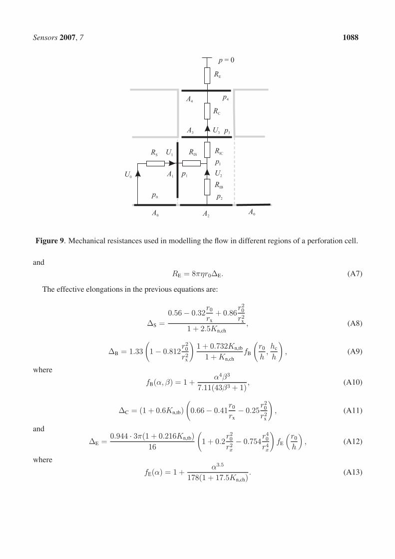
Figure 8 shows the topology of the cylindrical perforation cell, and Fig. 9 shows the lumped mechani-

cal resistances used in modelling the flow resistance of the cell. The flow resistanceRp of the perforation

cell consists of lumped flow resistances and their effective elongations. The equations have been derived

partly analytically and partly by fitting the model to FEM simulations by varying the coefficients in

heuristic equations [10].

The mechanical resistance of the perforation cell is [11]

Rp = RS +RIS +RIB +r4xr40(RIC +RC +RE) , (A1)

where rx and r0 are the outer and inner radii of the cylindrical perforation cell, respectively.

The lumped resistances are

RS =12πηr4xQchh3

(1

2lnrx

r0−3

8+r202r2x−r408r4x,

)(A2)

RIS =6πη(r2x − r

20)2

r0h2∆S, (A3)

RIB = 8πηr0∆B, (A4)

RIC = 8πηr0∆C, (A5)

RC =8πηhc

Qtb, (A6)

Sensors 2007, 7 1088

RS

RC

A0 A2

A3

A4

RIS

A0

pI

RE

U3

U2

U1

U0

p0

A1

p = 0

p1

RIC

p2

RIB

p3

p4

Figure 9. Mechanical resistances used in modelling the flow in different regions of a perforation cell.

and

RE = 8πηr0∆E. (A7)

The effective elongations in the previous equations are:

∆S =

0.56− 0.32r0rx+ 0.86

r20r2x

1 + 2.5Kn,ch, (A8)

∆B = 1.33

(1− 0.812

r20r2x

)1 + 0.732Kn,tb

1 +Kn,chfB

(r0h,hc

h

), (A9)

where

fB(α, β) = 1 +α4β3

7.11(43β3 + 1), (A10)

∆C = (1 + 0.6Kn,tb)

(0.66− 0.41

r0

rx− 0.25

r20r2x

), (A11)

and

∆E =0.944 · 3π(1 + 0.216Kn,tb)

16

(1 + 0.2

r20r2x− 0.754

r40r4x

)fE

(r0

h

), (A12)

where

fE(α) = 1 +α3.5

178(1 + 17.5Kn,ch). (A13)

Sensors 2007, 7 1089

References

1. Pedersen, M.; Olthuis, W.; Bergveld, P. A silicon condenser microphone with polyamide diaphragm

and backplate. Sensors and Actuators A 1997, 63, 97–104.

2. Goldsmith, C. L.; Malczewski, A.; Yao, Z. J.; Chen, S.; Ehmke, J.; Hindel, D. H. RF MEMs variable

capacitors for tuneable filters. Int J RF and Microwave CAE 1999, 9, 362–374.

3. Dec, A.; Suyama, K. Micromachined electro-mechanically tuneable capacitors and their application

to RF ICs. IEEE Transactions on Microwave Theory and Techniques 1998, 46(12), 2587–2596.

4. Mattila, T.; Hakkinen, P.; Jaakkola, O.; Kiihamaki, J.; Kyynarainen, J.; Oja, A.; Seppa, H.; Seppala,

P.; Sillanpaa, T. Air damping in resonant micromechanical capacitive sensors. In 14th European

Conference on Solid-State Transducers, EUROSENSORS XIV, pages 221–224, Copenhagen, 2000.

5. Starr, J. B. Squeeze-film damping in solid state accelerometers. In Solid-State Sensor and Actuator

Workshop, IEEE, pages 44–47, Hilton Head Island, 1990.

6. Kim, E.-S.; Cho, Y.-H.; Kim, M.-U. Effect of holes and edges on the squeeze film damping of

perforated micromechanical structures. In Proc. of IEEE Micro Electro Mechanical Systems Conf.,

pages 296–301, 1999.

7. Veijola, T.; Pursula, A.; Raback, P. Extending the validity of existing squeezed-film damper models

with elongations of surface dimensions. Journal of Micromechanics and Microengineering 2005,

15, 1624–1636.

8. Skvor, Z. On the acoustical resistance due to viscous losses in the air gap of electrostatic transducers.

Acustica 1967, 19, 295–299.

9. Homentcovschi, D.; Miles, R. N. Viscous damping of perforated planar micromechanical structures.

Sensors and Actuators A 2005, 119, 544–552.

10. Veijola, T. Analytic damping model for an MEM perforation cell. Microfluidics and Nanofluidics

2006, 2(3), 249–260.

11. Veijola, T. Analytic damping model for a square perforation cell. In Proceedings of the 9th

International Conference on Modeling and Simulation of Microsystems, volume 3, pages 554–557,

Boston, 2006.

12. Veijola, T.; Mattila, T. Compact squeezed-film damping model for perforated surface. In Proceed-

ings of Transducers’01, pages 1506–1509, Munich, Germany, 2001.

13. Yang, Y.-J.; Yu, C.-J. Macromodel extraction of gas damping effects for perforated surfaces with

arbitrarily-shaped geometries. In Proceedings of the 5th International Conference on Modeling and

Simulation of Microsystems, pages 178–181, San Juan, PR, 2002.

14. Bao, M.; Yang, H.; Sun, Y.; French, P. J. Modified Reynolds equation and analytical analysis of

squeeze-film air damping of perforated structures. Journal of Micromechanics and Microengineer-

ing 2003, 13, 795–800.

15. Bao, M.; Yang, H.; Sun, Y.; Wang, Y. Squeeze-film air damping of thick hole-plate. Sensors and

Actuators A 2003, 108, 212–217.

16. Raback, P.; Pursula, A.; Junttila, V.; Veijola, T. Hierarchical finite element simulation of perforated

plates with arbitrary hole geometry. In Proceedings of the 6th International Conference on Modeling

and Simulation of Microsystems, volume 1, pages 194–197, San Francisco, 2003.

Sensors 2007, 7 1090

17. Sattler, R.; Wachutka, G. Analytical compact models for squeezed-film damping. In Symposium on

Design, Test, Integration and Packaging of MEMS/MOEMS, DTIP 2004, pages 377–382, Montreux,

2004.

18. da Silva, M. G.; Deshpande, M.; Greiner, K.; Gilbert, J. R. Gas damping and spring effects on

MEMS devices with multiple perforations and multiple gaps. In Proceedings of Transducers’99,

volume 2, pages 1148–1151, Sendai, 1999.

19. Homentcovschi, D.; Miles, R. N. Modeling of viscous damping of perforated planar microstruc-

tures, applications in acoustics. Journal of the Acoustical Society of America 2004, 116, 2939–2947.

20. Kwok, P. Y.; Weinberg, M. S.; Breuer, K. S. Fluid effects in vibrating micromachined structures.

Journal of Microelectromechanical Systems 2005, 14(4), 770–781.

21. Veijola, T.; Raback, P. A method for solving arbitrary MEMS perforation problems with rare

gas effects. In Proceedings of the 8th International Conference on Modeling and Simulation of

Microsystems, volume 3, pages 561–564, Anaheim, 2005.

22. Gross, W. A. Gas Film Lubrication. Wiley, New York, 1962.

23. Veijola, T.; Kuisma, H.; Lahdenpera, J.; Ryhanen, T. Equivalent circuit model of the squeezed gas

film in a silicon accelerometer. Sensors and Actuators A 1995, 48, 239–248.

24. Karniadakis, G. E.; Beskok, A. Micro Flows, Fundamentals and Simulation. Springer, Heidelberg,

2002.

25. Ebert, W. A.; Sparrow, E. M. Slip flow in rectangular and annular ducts. Journal of Basic Engi-

neering, Trans. ASME 1965, 87, 1018–1024.

26. Mortensen, N. A.; Okkels, F.; Bruus, H. Reexamination of Hagen-Poiseuille flow: Shape-dependence

of the hydraulic resistance in microchannels. Phys. Rev. E 2005, 71, 057301.

27. Elmer. Elmer – finite element solver for multiphysical problems, 2006. http://www.csc.fi/elmer.

c© 2007 by MDPI (http://www.mdpi.org). Reproduction is permitted for noncommercial purposes.