Methods and Models in Preparing Weapon-Target Interaction Data for Combat Simulations

Oleg Mazonka and Denis Shine

Defence Science and Technology Organisation Email: oleg.mazonka@dsto.defence.gov.au; denis.shine@dsto.defence.gov.au

Abstract: Combat simulations are part of a suite of tools used by Defence Science and Technology Organisation (DSTO) to support Army decision makers, allowing analysis of the effects of changes in equipment, tactics or force structure. In order to represent combat effectively, these tools require enormous amounts of input data, which cannot be gained from empirical sources. This input data must cover aspects such as detection and identification of targets, behavioral decision making, basic system capabilities and weapon/target interactions. This data is represented within these combat simulations as lookup tables, from which an appropriate result, or probability of a result, is selected.

Our approach (Mazonka, 2012) seeks to provide fit-for-purpose vulnerability and lethality data to allow these simulations to adjudicate the outcomes of combat. This approach takes simple physical data from weapon and target systems and applies physics models to determine the probabilistic results of their interactions. We are cognisant of a number of limitations: the paucity of available empirical data, short lead times for data requirements and a requirement for an extremely broad set of interaction data, at the expense of depth.

In this paper we briefly describe our solutions to problems of armour penetration, probability propagation and blast effects, along with methods for converting generic result data such as vehicle probability of kill models into simulation-specific input data. These solutions are presented as a series of limited, low level methods, which illustrate some of the challenges inherent in generating fit-for-purpose combat simulation data.

Keywords: Combat Simulation, Performance Modeling, Data Generation, Applied Mathematics

20th International Congress on Modelling and Simulation, Adelaide, Australia, 1–6 December 2013 www.mssanz.org.au/modsim2013

1047

Oleg Mazonka and Denis Shine, Methods and Models in Preparing Weapon-Target Interaction Data for Combat Simulations

1. INTRODUCTION

Land Operations Research (LOR) is undertaking a concerted effort to develop methods to generate fit-for-purpose performance data for use within combat simulations. Our general approach (Mazonka, 2012) is based heavily on similar work (see for example Cazzolato (2006) and Cazzolato (2007)), which describes methods for generating data suitable for the Joint Conflict and Tactical Simulation (JCATS) wargame. While the LOR simulation suite is similar in some respects to JCATS, its format requirements and interpretation of input data are different enough that we have been required to develop a number of models and techniques in order to properly represent weapon-target interaction within these combat simulations. This paper describes some of the more interesting problems we have encountered, along with our solutions.

2. METHOD

Our approach seeks to provide fit-for-purpose data for a wide range of interactions between military systems and is divided into three core models:

- A Ballistics and Dispersion model which can predict trajectories, armour penetration and ballistic errors for a broad range of weapons systems

- A Direct Fire model which determines the probability of kill for direct fire weapons (such as a rifle or tank cannon) against infantry and vehicle targets; and

- An Indirect Fire model which determines the probability of kill for a high explosive shell (such as a mortar bomb or grenade) detonating near an infantry or vehicle target

Each model shares components and source data. The ballistics model provides trajectory data that is used directly by combat simulations, but also feeds the other two models vital information such as penetration and dispersion, so that they can generate their own combat simulation input data. The direct and indirect fire models both use the same target format and both use the concept of a Kill Grid to assess damage to targets. Each of these concepts is explained within Mazonka (2012). Finally, we note that for this paper, we separate the definition of direct and indirect fire only in terms of their terminal effect, not in terms of fly-out.

This approach is part of an effort to develop a fully integrated data generation solution for our suite of combat simulations. The Simulation Repository (SimR) (Angel et al, 2011) is being built to serve as the storage mechanism for combat simulation input data. SimR includes a capability for rating the provenance or accuracy of sourced data and the ability to produce the detailed, interconnected data files that combat simulations require, all available through a graphical user interface. Our vulnerability and lethality modeling serves as a tool SimR can call upon to generate more complex data types, such as those described above.

3. PENETRATION, PROPAGATION AND FRAGMENTS

In this section we present two topics. We first present models for armour penetration and the propagation of probabilities of kill produced by projectiles penetrating armour. These models allow for the prediction of the effect of a single penetrator or high explosive fragment on a target. Given this penetration model, we then present our solution for combining the many potential probabilistic kill results produced when a high explosive bomb produces many fragments.

3.1. Armour Penetration & Propagation

Armour Penetration is a topic studied in great detail and subsequently there is a large volume of literature detailing equations and models that predict penetration characteristics. Such models are often tailored to a particular weapons system, target type or set of environmental conditions, which provides an excellent depth of knowledge, but with limited applicability to other situations. Cazzolato (2006) provides an excellent set of applicable models that describe the majority of anti-armour weapons with a relatively small input data requirement. Table 1 summarises the key models used and their applicability to different battlefield weapon types.

Table 1. Penetration Models (Cazzolato, 2006)

Weapon Model Name Input Parameters Small Arms

High Explosive Fragments Grabarek Mass (m), Diameter (D), Constant Cg

Large Calibre Machine Guns Auto Cannons

Lambert Mass (m), Diameter (D), Length (L),

Angle of Impact (θ )

1048

Oleg Mazonka and Denis Shine, Methods and Models in Preparing Weapon-Target Interaction Data for Combat Simulations

Discarding Sabot Rounds Subramanian &

Bless Diameter (D), Length (L),

Constants A, b, c

Shaped Charges HEAT Round

Equation Jet Length (L), Copper Density ( lρ ),

Target Density ( tρ )

Each equation provides a final result d, which is the penetration (in mm) of Rolled Homogenous Armour (RHA) equivalent of this projectile, given its parameters and a supplied velocity v. This penetration value can then be compared to an armour plate, which is given a thickness, also in RHA. Computing the result of this interaction is not a binary case and Cazzolato (2007) presents a simple model for determining the probability of penetration, given a target thickness of t:

( )

≤<<−

≥=

92.0if0

08.192.0if16.092.0

08.1if1

)npenetratio(

td

tdtd

td

P

This equation, along with the appropriate penetration equation, defines the probability of penetration for a single projectile-on-armour event. However, actual targets will usually have multiple components, several of which may be intersected by the passing projectile. In our system, targets are represented as 3D models with armour levels attached to groups of geometry, along with a resultant type of kill if this component is penetrated. As described in Mazonka (2012), our vulnerability models use a Kill Grid, which is a plane of equal-sized cells overlaid on the target perpendicular to the line of fire. The projectile is “fired” through each cell and a result is returned, giving probabilities of Mobility (M), Firepower (F), Mobility/Firepower (S) and Catastrophic (K) Kills if this projectile passes through this cell. This representation is a widely used system in the vulnerability modeling community (see for example Haskell (1973)), and used by most of our combat simulations. Calculating the final probability P is a non-trivial task, since as it passes through each component of the vehicle, it has a probability of either:

- Penetrating the component and thus having some effect on the target – P(M/F/S/K) - Penetrating the component but having no effect on the target – P(N) - Failing to penetrate the component – P(ZN), which also has no effect. - As multiple components are penetrated one can also get P(ZX), which has the effect X (one of

M/F/S/K) but failed to penetrate the last component.

Combining the results of two or more components can be done by considering these probabilities sequentially. This introduces four other probabilities, since a projectile can fail to penetrate a component, but still have an effect from penetrating previous components. A new probability set is combined with an existing one using the matrix shown in Table 2, which takes into account some implications of combining kill types: M and F becomes S, S and M or F becomes S, and anything and K becomes K.

This table defines the appropriate groups of kill events happening in sequence. For example, the new probability for a Mobility/Firepower kill must be calculated as:

( ) ( ) ( ) Sold

NNSFMold

SMSold

FFSold

Mnew

S PPPPPPPPPPPPPP ++++++++=

with oldFP being the probability calculated up to the current penetration event (left most column) and PM

being probability of the current (top row). This value is calculated by the sum of joint probabilities of corresponding cells in Table 2. Since both sets of probabilities are mutually exclusive and jointly exhaustive, the new probability set will automatically normalise to 1.

For each piece of geometry the projectile may pass through, the combination above is performed. Once the penetration power of the projectile is exhausted, or it has passed completely through the target, the final probability is calculated as a sum of penetrated and non-penetrated values – for example P(M) is PM + PZM. This method is applied to give the result of one projectile or fragment intersecting a target, given a specified

Table 2. Combining Probabilities

New Probability Set

PM PF PS PK PN PZN

Exi

stin

g P

roba

bili

ty S

et PM M S S K M ZM

PF S F S K F ZF PS S S S K S ZS PK K K K K K ZK PN M F S K N ZN PZM ZM ZM ZM ZM ZM ZM PZF ZF ZF ZF ZF ZF ZF PZS ZS ZS ZS ZS ZS ZS PZK ZK ZK ZK ZK ZK ZK PZN ZN ZN ZN ZN ZN ZN

1049

Oleg Mazonka and Denis Shine, Methods and Models in Preparing Weapon-Target Interaction Data for Combat Simulations

trajectory vector and is calculated for each cell within a Kill Grid. From here, further methods are applied to combine the many individual results within a Kill Grid into one final probability of kill.

3.2. Human Targets – Penetration or Kinetic Energy?

Armour penetration sufficiently defines kill probabilities for vehicles hit by kinetic projectiles or fragments of high explosives. In the case when an explosive fragment hits a human, a method for obtaining a kill probability is unclear. Logically, the armour penetration model described previously can be applied to human targets, with the armour comprising body armour, clothes and skin. However, some models use the kinetic energy of the fragment to determine the incapacitation probability (US Army, 2010). Our approach is to calculate both penetration and kinetic energy kill probabilities (and their combinations of logical and and logical or), leaving blending the probabilities to another human study model.

3.3. Fragmentation effects

High explosive weapons produce three types of effect: air blast – damaging air pressure; translation – kinetic energy passed to objects or humans; and fragmentation. In Mazonka (2012) we described briefly all three effects. Here we touch on fragmentation in more detail.

The armour penetration model described in Section 3.1 can be used to calculate the probabilities of individual fragments produced by an explosion having some effect on a target. Thus the key problem here is combining the kill probabilities for many different fragment sizes while taking into account the physical properties of the fragments such as their distribution, velocities, shapes and material densities. Obviously the physical properties of fragments can be described only in a statistical manner with appropriate models. We use two common models that are most appropriate for simplified cases. Mott theory (Mott, 1943) is a model for describing the distribution of fragment sizes for an explosion, while Gurney (Cooper, 1996) describes a method for obtaining the initial velocity of such fragments

−=

AA M

m

mMmn exp

2

1)(

WM

Gv

C+=

5.00

where n(m) is fragment distribution by mass m, MA is a Mott constant depending on physical properties of the explosive casing of mass MC and the type of the explosive charge of mass W, v0 is the initial velocity of the fragments, G is the gurney constant depending on the type of the charge. Velocities of the fragments at the point of the impact with the target are reduced by the air drag and can be further calculated knowing the drag factor.

If we know the distribution of fragment sizes and their velocities, the problem is now one of how to combine these probabilities. If we make the following assumptions to simplify the initial problem:

1) the fragments are distributed spherically with a uniform probability, 2) the kill event does not depend on the position of the fragment hitting the target, and 3) only one type of the kill event is considered,

the cumulative probability for all fragments can be found by

( ) ( )( )∞

−−=0

1lnexp1 dmmPFmnNP erT

(1)

as shown in Mazonka (2013), where P is the cumulative probability, NT is the total number of fragments deduced from the Mott equation, Fr is the probability of an individual fragment hitting the target, and Pe is the probability of the kill event given hit.

Assuming a spherically uniform fragment distribution is not realistically appropriate. The real distributions of fragments for military explosives are usually axially symmetric but not spherically uniform. This becomes obvious in the extreme case when all fragments are thrown in one direction. We simulate the asymmetry in the fragment distribution using an assumption that fragments are distributed uniformly within a solid angle. That can be governed by a single parameter α – the fraction of the sphere covered by that solid angle. In this case the geometrical probability of hit Fr is

( ) ( )παθθ

4T

Tr

SF =

where θT is the angle of the direction of the explosion, and S is the solid angle of target covered by the solid angle of distributed fragments. In our model the angle θT is never assumed to be known and thus the cumulative probability in the equation (1) above transforms into:

1050

Oleg Mazonka and Denis Shine, Methods and Models in Preparing Weapon-Target Interaction Data for Combat Simulations

( ) ( ) ( )( ) ∞

−−=π

α θθθ0 0

1lnexpsin2

11 mPFmndmNdP eTrTTT

(2)

where index α specifies the selected asymmetry parameter. For general bombs an estimate of the parameter based on fragmentation patterns is 0.8, although that is yet to be thoroughly validated by empirical data.

The second assumption accompanying equation (1) can be dropped by introducing a dependency of Pe on orientation of the target in respect to the orientation of the explosion. If fragments can produce different level of kill probabilities depending on the position of the hit, then three extra dimensions have to be added into consideration. First, the axial symmetry of the fragment distribution cannot be cancelled since different axial angles φ with fixed Tθ result in different kill probabilities. Second, two dimensions θ and ϕ are added to

the calculation to take into account different points of hit. Because eP depends on four angles and the mass of

the fragment, both factors Fr and Pe can be combined into ( )φθϕθ ,,,, Te mP . The resulting expression for

cumulative probability becomes (with omitted arguments):

( )( )

−−=

∞ −

0

2

0

21arccos

00

2

0

sin4

11lnexpsin

4

11

παππ

ϕθθπα

θθφπ eTTT PddmndmNddP

(3)

A detailed derivation can be found at Mazonka (2013). The fact that only 4 angular dimensions present in the integral can be explained simply. Both target and oriented explosion must be described by 6 angles: 3 each. One angle can be removed according to that the distribution of the fragment explosion is within a cone, and a cone is symmetric around its axis. The second dimension disappears because the coordinate system can be oriented in a direction of target or explosion cone without losing generality.

This leaves us with the final assumption of equation (1), that only one kill event is considered, which as shown in Section 4.1, is not true. We must consider the possibility of Mobility (M), Firepower (F), Mobility/Firepower (S) and Catastrophic (K) Kill types, along with the probability of no effect (N), along with their previously described hierarchy and interdependencies. After proper decomposition of dependencies between the different types of events, equation (3) becomes:

( )( )

−−=

∞ −

0

2

0

][21arccos

00

2

0

][ sin4

11lnexpsin

4

11

παππ

ϕθθπα

θθφπ

ieTTT

i PddmndmNddP

(4)

where mass and angle arguments are omitted and initial and final probabilities are defined as

][]3[

][][][]2[

][][][]1[

][][][][]0[

Kee

Ke

Se

Mee

Ke

Se

Fee

Ke

Se

Fe

Mee

PP

PPPP

PPPP

PPPPP

=

++=

++=

+++=

(5)

]3[][

]3[]0[]2[]1[][

]2[]0[][

]1[]0[][

PP

PPPPP

PPP

PPP

K

S

F

M

=

−−+=−=

−=

(6)

Calculations are done in three steps ][][][][ Xiie

Xe PPPP →→→ by equations (6), (4), and (5) correspondingly.

Equations (4-6) describe the calculation of cumulative probability of kill for all fragments in the explosion. If all three assumptions of equation (1) are satisfied then it reduces to equation (1).

4. OUTPUT CONVERSION

Section 3 described some of the more interesting problems and solutions that we have encountered as we attempt to generate simulation input data. Ultimately the goal of our work is to produce data that is not only relevant to combat simulations, but correctly formatted and interpreted by the simulation. In this section we present two cases that illustrate why this process is not always straightforward.

4.1. Individual Unit of Action Data

The COMBAT XXI (Kunde 2005) and One Semi-Automated Forces (OneSAF) (PM OneSAF, 2012) simulations are designed to source their data from the Army Materiel Systems Analysis Activity (AMSAA) organisation, which conducts systems analysis for a number of purposes, including the generation of data for combat simulations. Data for direct fire weapons against vehicles is described in a format called the Individual Unit of Action (IUA) format, which provides the probability of damaging a target given a hit. Since both COMBAT XXI and OneSAF both support the IUA format, it is reasonable to assume that one could provide the same IUA file to each, however we have found that this is not the case, which necessitates

1051

Oleg Mazonka and Denis Shine, Methods and Models in Preparing Weapon-Target Interaction Data for Combat Simulations

that we interpret and process the generic data in a Kill Grid differently depending on which simulation is the export target.

The IUA format provides for a number of engagement conditions, such as range, azimuth angle and target exposure, which are treated similarly by the two simulations. It also requires that the user specify kill results for a number of dispersions, from 1 foot to 10 feet from the center of the target. COMBAT XXI computes a hit location on the target and calculates its distance from the aim point, picking data from the appropriate dispersion value in the IUA file. This means that the IUA file must contain data for the probability of kill, given a hit, for a series of concentric rings emanating from the centre of the target. Generating this data from a Kill Grid is relatively simple – the data for each ring is the average result of all cells falling within this ring.

OneSAF does not use the actual hit location, except for determining if the target is hit in the first place. Instead it takes the calculated error of the weapon (which is expressed as a standard deviation), using the closest dispersion value in the IUA data. Therefore, each dispersion value must contain the probability of kill, given a hit, for a weapon with the specified error.

The key difference in these methods is that, shot-to-shot, the probability of kill in COMBAT XXI may change as the sampled hit point lands in different dispersion rings on the target, whereas in OneSAF, the kill probability, providing no other factors change, should remain the same. So therefore, while COMBATXXI and OneSAF use exactly the same IUA format, the data required is actually different due to the different interpretations of simulations. Figure 1 describes how each simulation interprets IUA data, along with the impact on our data generation process. Coloured cells on the left represent which cells are counted for the range ring. On the right, the normal distributions have a standard deviation matching the first range ring, after which each cell is weighted based on the distribution.

COMBAT XXI

When Adjudicating a Kill: Computes location of hit and selects data from appropriate dispersion. Data Generation Impact: Compute uniform average result for points within each concentric range ring.

OneSAF When Adjudicating a Kill: Takes weapon dispersion and samples from nearest IUA dispersion value. Data Generation Impact: Integrate a bivariate normal distribution over target with a standard deviation matching each dispersion value.

Figure 1. Interpretation of IUA Data - COMBAT XXI (left) vs OneSAF (right).

4.2. Lethal area

Our high explosive model produces generic data describing the probability of kill of an explosive at a specified Range, Angle and Elevation relative to a target. Despite this logical representation, few combat models use a format that is directly translatable from this paradigm and therefore we must make further approximations. We present two examples of this problem, along with our solutions.

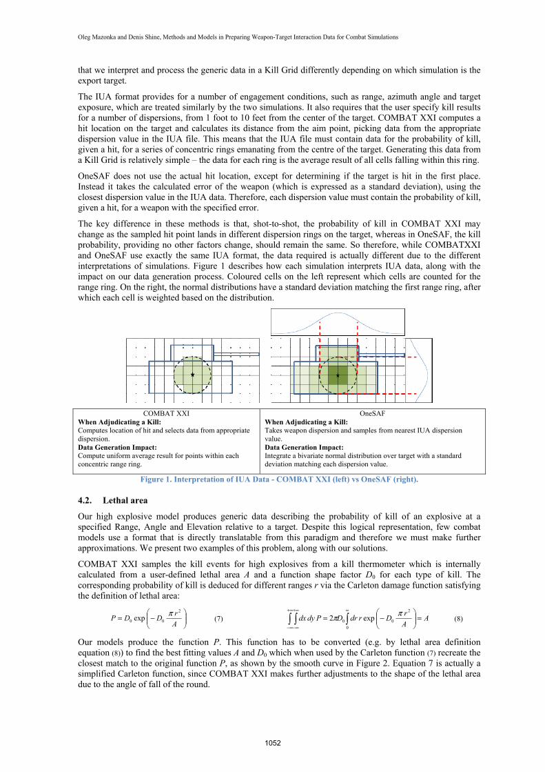
COMBAT XXI samples the kill events for high explosives from a kill thermometer which is internally calculated from a user-defined lethal area A and a function shape factor D0 for each type of kill. The corresponding probability of kill is deduced for different ranges r via the Carleton damage function satisfying the definition of lethal area:

−=

A

rDDP

2

00 expπ

(7) AA

rDrdrDPdydx =

−=

∞+∞

∞−

+∞

∞− 0

2

00 exp2ππ

(8)

Our models produce the function P. This function has to be converted (e.g. by lethal area definition equation (8)) to find the best fitting values A and D0 which when used by the Carleton function (7) recreate the closest match to the original function P, as shown by the smooth curve in Figure 2. Equation 7 is actually a simplified Carleton function, since COMBAT XXI makes further adjustments to the shape of the lethal area due to the angle of fall of the round.

1052

Oleg Mazonka and Denis Shine, Methods and Models in Preparing Weapon-Target Interaction Data for Combat Simulations

Our models assume no knowledge of the orientation of the round and thus our approximation techniques take the average for different aspect angles before deducing A.

As another case, the Close Action Environment (CAEn) (Bowley, 2004) takes as input a table of kill probabilities depending on distance between explosion and the target and the orientation of the target, between which probabilities are linearly interpolated. CAEn allows for only a limited number of such points, requiring that we down-sample the (usually much larger) set of points that were calculated within the high explosive model, again shown in Figure 2. This problem boils down to finding the minimum difference between the original and interpolated function by changing the points, both positions and values, which represent the interpolated function. Algorithms of finding minima in multidimensional space solve this problem.

5. CONCLUSION

This paper presented a set of interesting problems we have encountered in our work to develop fit-for-purpose vulnerability and lethality data for combat simulations. They serve to underline the fact that producing performance data useful for combat simulations requires not only appropriately representative physical models but also an understanding of how each combat simulation will ultimately interpret and use its input data. Our models at present show acceptable internal consistency – more protected targets are less vulnerable, more advanced munitions are more lethal and changing angles or ranges have appropriate effects. More work is required to appropriately validate our models against empirical data and more advanced vulnerability models.

REFERENCES

Angel, C., Eigenraam, J., Hemming, D., & Stone, B. (2011). SimR - Centralising Data Storage for Modelling and Simulation. SimTect 2011, Melbourne, Australia.

Bowley, D.K.; Castles, T.D.; Ryan, A. , (2004) Attrition and suppression, DSTO-TR-1638

Cazzolato, F., & Roy, R. L. (2006). Calculation of Ballistic Coefficients, Range Tables and Armour Penetration for use by JCATS (TM 2006-39): Centre for Operational Research and Analysis.

Cazzolato, F., Roy, R. L., Levesque, J., & Pond, G. (2007). Probabilities of Kill in JCATS (TM 2007-33): Centre for Operational Research and Analysis.

Cooper, P. W. (1996). Acceleration, Formation, and Flight of Fragments Wiley-VCH. pp. 385–394 Haskell, D. F., (1973) AVVAM-1 (Armored Vehicle Vulnerability Analysis Model), Vulnerability Sensitivity Studies Kunde, D., & Darken, C. J., (2005) Event Prediction for Modeling Mental Simulation in Naturalistic

Decision Making

Mazonka, O. & Shine, D. (2012). Simple Physical Models in Support of Vulnerability and Lethality Data for Wargaming and Simulation Environments, SimTect 2012, Adelaide, Australia.

Mazonka, O. (2013). Cumulative Probability of Blast Fragmentation Effect, arXiv:1305.2285.

Mott, N. F. (1943). Fragmentation of H.E. Shells: a Theoretical Formula for the Distribution of Weights of Fragments. Ministry of Supply.

PM OneSAF, U.S. Army PEO STRI Product Manager, (2012), http://www.onesaf.net/

US Army (2010). Common Risk Criteria Standards for National Test Ranges. Range Safety Group Risk Committee, U.S. Army White Sands Missile Range.

Figure 2. P(K) over range of BRDM-2 vehicle by 155mm M107 round. Red dots and connected with green lines represent probabilities calculated by our model. The smooth black line is the best fit of the Carleton function, while the other black line is a 5-point fit to conform with CAEn.

1053