Embed Size (px)
Citation preview

Methodologies of Early Detection ofStudent Dropouts
Ruta Gronskyte
Kongens Lyngby 2011IMM-M.Sc-2011-67

Technical University of DenmarkInformatics and Mathematical ModellingBuilding 321, DK-2800 Kongens Lyngby, DenmarkPhone +45 45253351, Fax +45 [email protected]
IMM-M.Sc: ISSN 1601-233X

Summary
The Danish government hopes to have more highly educated youngpeople in the future. However very high dropout rates especial from thetechnical subjects makes it difficult to achieve the goal. The TechnicalUniversity of Denmark is already trying to monitor the performance ofthe students, but the current method is not efficient enough. Monitoringstudents can raise an alarm to the administration about potential dropoutstudents. Helping potential dropouts might get them back on the trackfor graduation.
In this master’s thesis student dropouts from the Technical University ofDenmark is analysed. Several methods like the logistic regression, prin-cipal component logistic regression, classification and regression trees(CART), classification and regression trees bagging (CART bagging), ran-dom forest and multivariate adaptive regression splines are investigated.With each method a dropout detection system is built and compared. Formodel building and testing historical data is used.
CART and CART bagging performs significantly better than the others.Further analysis must be performed for tuning the final system. Incomparison to the current system all analysed models performs better.

ii

Resume
Den danske regering haber pa at have flere højtuddannede unge i fremti-den. Store frafald fra især de tekniske fag gør det svært at indfri malet.Danmarks Tekniske Universitet prøver allerede at overvage de stude-rendes resultater, men den nuværende metode er ikke effektiv nok.Overvagning af de studerende kan alamere administrationen om enstuderendes mulige frafald. En mulig frafaldende studerende kan hjæl-pes tilbage pa sporet sa de kan færdiggøre uddannelsen.
I det indeværende kandidatspeciale analyseres frafaldne studerende fraDanmarks Tekniske Universitet. En række metoder som logistisk regres-sion, principal komponent logistisk regression, klassifikations og regres-sionstræer (CART), klassifikations og regressionstræer bagging (CARTbagging), tilfældig skov, multivariat adaptiv regressionskilenoter un-dersøges. For alle metoder bygges og sammenlignes et system til atopdage frafald. Historisk data bruges til opbygningen af modellerne.
CART og CART bagging er signifikant bedre til at opdage frafald endnogen af de andre. Yderligere analyse skal til for at fintune det endeligesystem. Sammenlignet med det nuværende system er alle de analyseredemodeller bedre til at opdage frafald.

iv

Preface
This thesis was prepared at Informatics Mathematical Modelling, theTechnical University of Denmark in partial fulfillment of the require-ments for acquiring the Master of Science in Engineering (MathematicalModelling and Computation).
The thesis deals with different aspects of mathematical modelling ofsystems using data and partial knowledge about the structure of the sys-tems. The main focus is on modelling the student dropouts for detectionpurpose at DTU.

vi

Acknowledgements
This master’s thesis was done in collaboration with the Department forStudy Affairs at the Technical University of Denmark. I would like tothank Merete Reuss, Annette Elmue, Camilla Nørring and ChristianWestrup Jensen who provided the data and fruitful insight to the currentsystems in use.
I would like to thank Bjarne Kjær Ersbøll who offered this topic whenmy initial project turned out to be infeasible. Also a thank you for thesupport while writing this thesis.
A special thank you to my supervisor Murat Kulahci for his invaluablediscussions and help during the project.
Last but not least, thank you for Rune Juhl for his comments on my thesisand emotional support.

viii

Contents
Summary i
Resume iii
Preface v
Acknowledgements vii
1 Introduction 11.1 Overview of Student Drop Out in Denmark . . . . . . . . . 11.2 Current System at Technical University of Denmark . . . 21.3 Goal of this Master’s Thesis . . . . . . . . . . . . . . . . . 3
2 Principe of Quality Control 52.1 Reasons for Process Variations . . . . . . . . . . . . . . . . 52.2 Statistical Basics of the Control . . . . . . . . . . . . . . . . 72.3 Phase I and Phase II of Control Methods Application . . 9
3 Types of Scoring 113.1 Application Scoring . . . . . . . . . . . . . . . . . . . . . . . 113.2 Performance Scoring . . . . . . . . . . . . . . . . . . . . . 12
4 Techniques of Scoring 154.1 Logistic Regression . . . . . . . . . . . . . . . . . . . . . . 154.2 Principle Component Logistic Regression . . . . . . . . . . 174.3 Classification and Regression Tree . . . . . . . . . . . . . 18

x CONTENTS
4.4 CART and Bagging . . . . . . . . . . . . . . . . . . . . . . 244.5 Random Forest . . . . . . . . . . . . . . . . . . . . . . . . 244.6 Multivariate Adaptive Regression Splines . . . . . . . . . . 27
5 Data 29
6 Modelling 356.1 Modelling Techniques and Methods . . . . . . . . . . . . 356.2 Logistic Regression Modelling . . . . . . . . . . . . . . . . 386.3 Principle Component Analysis and Logistic Regression
Modelling . . . . . . . . . . . . . . . . . . . . . . . . . . . 406.4 CART Modelling . . . . . . . . . . . . . . . . . . . . . . . 446.5 Bagging Modelling . . . . . . . . . . . . . . . . . . . . . . . 516.6 Random Forest Modelling . . . . . . . . . . . . . . . . . . 546.7 MARS Modelling . . . . . . . . . . . . . . . . . . . . . . . 72
7 Result Analysis 777.1 Model Comparison . . . . . . . . . . . . . . . . . . . . . . . 777.2 Final CART Model Stability . . . . . . . . . . . . . . . . . 787.3 Important Variable Analysis . . . . . . . . . . . . . . . . . 80
8 Conclusion 838.1 Future Work . . . . . . . . . . . . . . . . . . . . . . . . . . 85
A LR Models for Every Semester 89A.1 LR: Model 1 . . . . . . . . . . . . . . . . . . . . . . . . . . 89A.2 LR: Model 2 . . . . . . . . . . . . . . . . . . . . . . . . . . 90A.3 LR: Model 3 . . . . . . . . . . . . . . . . . . . . . . . . . . . 91A.4 LR: Model 4 . . . . . . . . . . . . . . . . . . . . . . . . . . 92A.5 LR: Model 5 . . . . . . . . . . . . . . . . . . . . . . . . . . 93A.6 LR: Model 6 . . . . . . . . . . . . . . . . . . . . . . . . . . 96A.7 LR: Model 7 . . . . . . . . . . . . . . . . . . . . . . . . . . . 97A.8 LR: Model 8 . . . . . . . . . . . . . . . . . . . . . . . . . . 99
B CART Bagging Models for Every Semester 101B.1 CART Bagging: Model 1 . . . . . . . . . . . . . . . . . . . . 101B.2 CART Bagging: Model 2 . . . . . . . . . . . . . . . . . . . 102B.3 CART Bagging: Model 3 . . . . . . . . . . . . . . . . . . . 103B.4 CART Bagging: Model 4 . . . . . . . . . . . . . . . . . . . 104B.5 CART Bagging: Model 5 . . . . . . . . . . . . . . . . . . . 105

CONTENTS xi
B.6 CART Bagging: Model 6 . . . . . . . . . . . . . . . . . . . 106B.7 CART Bagging: Model 7 . . . . . . . . . . . . . . . . . . . . 107B.8 CART Bagging: Model 8 . . . . . . . . . . . . . . . . . . . 108
C MARS Models for Every Semester 111C.1 MARS: Model 1 . . . . . . . . . . . . . . . . . . . . . . . . . 111C.2 MARS: Model 2 . . . . . . . . . . . . . . . . . . . . . . . . 113C.3 MARS: Model 3 . . . . . . . . . . . . . . . . . . . . . . . . 114C.4 MARS: Model 4 . . . . . . . . . . . . . . . . . . . . . . . . 115C.5 MARS: Model 5 . . . . . . . . . . . . . . . . . . . . . . . . . 117C.6 MARS: Model 6 . . . . . . . . . . . . . . . . . . . . . . . . 118C.7 MASR: Model 7 . . . . . . . . . . . . . . . . . . . . . . . . 120C.8 MARS: Model 8 . . . . . . . . . . . . . . . . . . . . . . . . 122
D MATLAB Code 125D.1 File: Main.m . . . . . . . . . . . . . . . . . . . . . . . . . . 125D.2 File: Main LR.m . . . . . . . . . . . . . . . . . . . . . . . . 128D.3 File: Main PCA.m . . . . . . . . . . . . . . . . . . . . . . . . 129D.4 File: Main CART.m . . . . . . . . . . . . . . . . . . . . . . . . 131D.5 File: Main Bagging.m . . . . . . . . . . . . . . . . . . . . . 132D.6 File: Main RF.m . . . . . . . . . . . . . . . . . . . . . . . . 133D.7 File: Main MARS.m . . . . . . . . . . . . . . . . . . . . . . . 136D.8 Function: Round ECTS.m . . . . . . . . . . . . . . . . . . . 139D.9 Function: SortExamps.m . . . . . . . . . . . . . . . . . . . 139D.10 Function: Status.m . . . . . . . . . . . . . . . . . . . . . . . 141D.11 Function: PersonalInfo short.m . . . . . . . . . . . . . . . 141D.12 Function: PersonalInfo.m . . . . . . . . . . . . . . . . . . 143D.13 Function: PerformanceInformations.m . . . . . . . . . . 145D.14 Function: Table.m . . . . . . . . . . . . . . . . . . . . . . . 146D.15 Function: DataDivision.m . . . . . . . . . . . . . . . . . . . 147D.16 Function: Cost Plot.m . . . . . . . . . . . . . . . . . . . . 149D.17 Function: Prediction txt.m . . . . . . . . . . . . . . . . 150D.18 Function: Prediction num.m . . . . . . . . . . . . . . . . 150D.19 Function: FinalPrediction.m . . . . . . . . . . . . . . . . . 151D.20 Function: StepPrediction.m . . . . . . . . . . . . . . . . . 151D.21 Function: FinalEval.m . . . . . . . . . . . . . . . . . . . . 152D.22 Function: Records.m . . . . . . . . . . . . . . . . . . . . . 153D.23 Function: SSS.m . . . . . . . . . . . . . . . . . . . . . . . . 154D.24 Function: NumberSemester.m . . . . . . . . . . . . . . . . 156

xii CONTENTS
Bibliography 157

CHAPTER 1
Introduction
1.1 Overview of Student Drop Out in Denmark
Not all students who begin a university education graduates. Accordingto [15] around 30-40% of the students drop out or change their subject.This high dropout rate cost 200 millions Danish kroner for the taxpayers.
Recently the reasons for dropping out have been discussed. The DanishInstitute of Governmental Research (in Danish: Anvendt KommunalFor-skning) made a large survey [14] trying to identify the reasons of earlystudents’ drop out. Data from year 2000-2005 was analysed in this surveyand several reasons were identified for early students’ drop out. One ofmost significant reason for completing the studies is establishment status.That is married persons with children are more likely to finish their edu-cation. Also students who previously completed a higher education.However, those who previously tried and failed to complete a highereducation are more likely to drop out once again. Another importantreason for drop out is an ethnic minority background. According to [18]a student with an ethnic minority background is 2.6 times more likely

2 Introduction
to drop out. The reason is discrimination at the study institutions anda lack of possibilities to study at home. The last reason is identified asperformance at the beginning of studies.
Some universities are taking actions to identify students with higherrisks for dropping out. One of the suggested solutions is pre-admissioninterviews. This allows to find the really motivated students. However,this approach is highly costly at around 3000 Danish kroner per interview[15].
The objective of this master’s thesis is to research and build a model basedon the general data obtained from the application and performance datafrom each semester to identify students who are most likely to dropout. Potential dropouts could be interviewed to reinstate their motiva-tion. The identification of the potential dropouts could save money andprovide the opportunity for more motivated students. Thus increasingthe effectiveness of the universities and helping to achieve the nationalgoal that half of the young population would earn a higher education.
1.2 Current System at Technical University of Den-mark
Camilar Nørring from the Student Counselling (Studievejledningen) atthe Technical University of Denmark (DTU) from the Department ofEducation and Study Affairs (Afdelingen for Uddannelse og Studerende)gave a short introduction to the remedies suggested by the Ministry ofScience, Technology and Innovation (Ministeriet for Videnskab, Tekno-logi og Udvikling)(VTU) and how DTU have implemented it.
According to the VTU the universities must contact students who are 6months (equivalent to 30 ECTS credits) behind. In other words, studentswho have not passed any credits for one semester. These students mustbe offered counselling. However it is not specified how it should be. Forthe students who are more than 12 months (60 ECTS credits) behind mustbe offered an individual meeting with a counsellor.

1.3 Goal of this Master’s Thesis 3
Students at DTU who are behind by more than 6 months and less than 12months (30-59 ECTS credits) gets an invitation by e-mail for an individualtalk with a counsellor. Those who are more than 12 months (60 ECTScredits) behind receive an official invitation by mail. Furthermore, publicworkshops on study planning, how to avoid delays and how to get backon track are organised every semester by the study counsellors. Allstudents are invited to participate.
1.3 Goal of this Master’s Thesis
The goal of this master’s thesis is to re-evaluate the current studentdropout detection system using principles of quality control, applicationand performance scoring techniques. To compare several performancescoring techniques and evaluate whether an improved method can besuggested. Also, identify significant characteristics for dropout studentdetection. Finally, compare findings with the current system.

4 Introduction

CHAPTER 2
Principe of Quality Control
Experience have shown how important it is to keep track on the students’performance to proactively help students from delays or an eventualdrop out. Student monitoring is a continuous process and the basicphilosophy could be adopted from statistical process control. The basicprinciples of process control are discussed in [16].
2.1 Reasons for Process Variations
The are two main branches of variability appearing in a process. Thefirst type is caused by the process itself. It does not matter how well theprocess is designed, there will always be natural variability. Whole ofnatural causes in the process is called stable system of change causes and theprocess that operates only with chance causes of variation present is saidto be in statistical quality control. Second type of variability sources are:improperly adjusted or controlled mechanisms, administration errors ordefected raw material. Whole of unnatural courses are called assignable

6 Principe of Quality Control
causes. Variability emerged from assignable causes usually is representedas unexceptionable outcome. A process that is operating in the presenceof the assignable causes is said to-be-out-of control.
It is noticed, that students who wants to graduate on time tend to study ina more stable manner than those unsure about their wishes and choices.However, sometimes even good students might go through a periodwhere the studies are quite difficult. This can be because of study, uni-versity and personal matters. Study or university related matters couldbe:
• changes at the university education system
• changes at the teaching methodology
• more difficult subjects in some period of studies then usual
• ...
Personal matters could be:
• changes in personal life
• health issues
• lack of concentration for any number of reasons
• ...
These reasons will degrade the overall performance of a student who willhowever eventually graduate. The assignable causes influence studentperformance much stronger and eventually the student will drop out.As previously discussed in chapter 1 on page 1 there are two types ofassignable causes: one related to university and studies and the other topersonal matters.

2.2 Statistical Basics of the Control 7
2.2 Statistical Basics of the Control
Control charts are widely used in the manufacturing industry. The ideais to take a sample of the manufactured product and compare it withthe target measurements. The changes over time are observed. Usingdifferent statistical techniques bounds can be set for the measurementvariations. While monitoring changes in the measurements, problems canbe detected and action can be taken to prevent producing non qualitativeproducts.
Classical control charts in student performance monitoring is not suit-able. There are many variables that can be used for monitoring. Thisproblem is quite usual in process control, thus combined variable chartsare used. It is not know which performance measurements should beused in student performance monitoring. In this master’s thesis a newperformance monitoring system is suggested. Students performance ismeasured every semester, which is the sampling time. Instead of chartspresenting the overall production performance chart status update willbe used. When the model detects a student not performing good enoughto graduate the student’s status is changed from “pass” to “drop out”.When the student is classified as “drop out” the assignable causes mustbe investigated so the student can be helped to perform better in thefuture. A simplified model scheme is presented in fig. 2.1. As it can be
...1 semester 2 semester n semester
General information
General information+
1 semester results...
General information+
n-1 semester resultsInformation
Conditions
Status
Model 1 Model 2 Model... Model n
Figure 2.1: Simplified model scheme.
seen in fig. 2.1 the model consists of n models. Every model analyse thegeneral information and student performance records from the previous

8 Principe of Quality Control
semester. The outcome of every model is the predicted student statusafter the mth, that m = 1, ..., n semester.
In process control where classical control charts are used it is often usedprobabilities of error type I and II. The type I error is indicating the prob-ability that the process is out of control when it is actually in control.The type II error is indicating the probability that the process is in controlwhen it is actually out of control. The sum of these errors is always equalto one thus decreasing one type error will increase the other. It is alwaysimportant to find the balance between these errors. For example, if thetype I error is very high false alarms will be occur too often. Likewise ahigh type II error will give the impression that the process in control. Inthe suggested model, the type I error is the classification of students asdropouts when they actually do pass. This error is also called false alarm.Error type II is when a student is classified as passed but actually is adropout.
The most important task of process control is to stabilise and improvethe process. To achieve this three basic ideas can be used:
1 Most processes are not in total statistical control.
2 Actions must be taken as soon as it is identified that process is outof control.
3 When actions are taken after control has been lost and an investiga-tion of the assignable causes is performed and the causes notified,a trend might be noticed.
As soon as a drop out student is identified using these three basic ideasan investigation must be performed. This will help to identity the prob-lems the student is facing and the university may be able to help him.Collecting the assignable causes might suggest what actions could betaken to prevent students from droping out and also improve the model.

2.3 Phase I and Phase II of Control Methods Application 9
2.3 Phase I and Phase II of Control Methods Applic-ation
Model building takes to distinct phases. In phase I the general processbehaviour is investigated. Usually it is assumed that the process is outof control and a general investigation is conducted to bring the processback to control. Usually already collected data is investigated. In phase IIthe suggested model is implemented and the process is followed online.During this phase it is assumed that the process is already in control.New adjustments might be implemented.
This master’s thesis is like a phase I. Already collected data is investigated.A general model is going to be suggested. Phase II is not a part of thisthesis and is suggested as future work. The phase II is as important as thephase I. In this case some of the students’ behaviour might change dueto the close monitoring of students. It might be necessary to re-estimatethe models or even redo the entire modelling.

10 Principe of Quality Control

CHAPTER 3
Types of Scoring
3.1 Application Scoring
Application scoring is wildly used in marketing. The aim of applicationscoring methods are to identify customers who a company can offer theirproducts or services to. For example resellers can target their advertise-ments for new products to a specific segment of the costumers. That isthose most likely to buy new products. Banks can use the informationfrom the applications for identifying those customers who are most likelyto keep up with their repayments. In bank terminology these methodsare usually called credit scoring. In this thesis application scoring methodis used to identify students who are most likely to drop out based ontheir application information even though these students are alreadyenrolled.
Usually the predictive variables are called characteristics and the valueor class they are assigned is called the attributes. The aim of applicationscoring is to build a model that could predict attribute classes using theavailable characteristics. There are several techniques developed over the

12 Types of Scoring
years and a broad overview is presented in [6]. Classical methods usedthese days are discriminant analysis and linear regression. Discriminantanalysis might have problems with data that do not follow the normaldistribution or groups that do not have a discrete form. Yet there aresome proposed solution for these problems. Linear regression can be usedfor two class identification. The benefit of linear regression is that it canbe used as application scoring and behavioural scoring which will be moreintroduced in section 3.2. Closely related to linear regression is logisticregression that may be also used in two discrete class classification. It isnoticed that it do not perform significantly better than linear regression.Another classical method is decision trees. The advantage of this methodis that non-linearity and interaction can be included in the model. Moreon CART in section 4.3 on page 18.
Other methods as mathematical programming, neural networks, nearest neigh-bour can be also used. Mathematical programming suffer from problemswith linear relations among the characteristics. Neural networks usedwith association rule is widely discussed in [9] and presented as one ofthe advanced classification methods. Yet using this method the interpret-ation of the model can be lost. Nearest neighbour avoid the distributionchange problem, though this method is highly computational expensive.
3.2 Performance Scoring
In many cases it is important to follow the performance of the customersto make sure that they will perform as expected at the application scoringlevel. This method is called performance or behavioural scoring. Applic-ation scoring is a more general technique that is done at the first step.Performance scoring evaluates existing customers based on the similarprinciples as application scoring. As in application scoring customerscan be classified to the same or a different performance group.
There are several common techniques between application and perform-ance scoring: linear/multiple discriminant analysis, linear regression, logisticregression, neural network and support vector machines all discussed in [9]and [8]. The same techniques can be used in application scoring. In

3.2 Performance Scoring 13
the discussion of these papers the linear discriminant analysis do notperform any better than any other methods. Support vector machinehas issues with parameter selection. As in application scoring neuralnetworks performs best.

14 Types of Scoring

CHAPTER 4
Techniques of Scoring
4.1 Logistic Regression
Logistic regression (LR) is one of the basic methods for the classificationproblem. The method is defining a non-linear relationship between thedependent and independent variables. LR can be used as a classifier withtwo or more classes. In biostatistical applications as in survival analysisLR is widely used due to its good performance in two class problems.The theory is discussed in [7].
4.1.1 Principles of the Logistic Regression
LR uses posterior probabilities of the K classes via a linear function in x.The model is naturally constrained so the probabilities are in the interval[0, 1] and sum to 1. The model is defined by K− 1 logit transformations

16 Techniques of Scoring
of the ratio of probabilities of two classes
logPr(G = 1|X = x)Pr(G = K|X = x)
= β10 + βT1 x (4.1)
logPr(G = 2|X = x)Pr(G = K|X = x)
= β20 + βT2 x
...
logPr(G = K− 1|X = x)
Pr(G = K|X = x)= β(K−1)0 + βT
K−1x.
Class K is arbitrarily chosen as a reference class and appears in the denom-inator in eq. (4.1). Hereafter the following notation for the probabilities isused: Pr(G = k|X = x) = pk(x; θ), where θ = {β10, βT
1 , ..., β(K−1)0, βTK−1}.
4.1.2 Estimating the Logistic Regression Model
Fitting logistic regression to data is solved by maximizing the conditionallikelihood of G given X. The log-likelihood for N observations is
l(θ) =N
∑i=1
log pgi(xi; θ). (4.2)
Maximizing the log-likelihood for the two classes problem is done bythe iteratively re-weighted least squares method. It is based on the Newton-Raphson algorithm which requires the Hessian matrix. Each iterationperforms a minimization and update the β estimate
βnew ← arg minβ
(z− Xβ)TW(z− Xβ). (4.3)
W is an NxN diagonal matrix of weights where the ith diagonal elementis p(xi; βold)(1− p(xi; βold)). z is the adjusted response
z = Xβold + W−1(y− p). (4.4)
Usually the best starting values is β = 0 and in most of the cases thealgorithm will converge.

4.2 Principle Component Logistic Regression 17
4.2 Principle Component Logistic Regression
Linear regression face problems with collinearity among variables. Oneoption is to remove insignificant variables and perform linear regres-sion in a smaller variable space. To select variables a principle componentanalysis (PCA) can be used [4]. [1] discuss two methods principle com-ponents logistic regression (PC-LR) and partial least-square logistic regression(PLS-LR) for dimension reduction in a logistic regression setting. As itis noticed in this paper, it can be expected that PC-LR will give betterestimates for regression coefficients. Thus PC-LR will be used in thisthesis.
4.2.1 Principles of Principle Component Analysis
The principle components is the best linear approximation of the space<p in the smaller space of the dimension q such that q ≤ p. The linearapproximation can be expressed as
f (λ) = µ + Vqλ. (4.5)
µ is the location vector which is the origo of the new coordinate spacein the original space <p. The q orthogonal unit vectors spanning thesubspace is arranged column wise in the loading matrix Vq. The matrix ispxq of size. It is how the PCs are weighted by the original space. λ is avector with q elements which is the point in the subspace - also called thescore. The scores from each observation is arranged in the score matrix.
The principle components are arranged by how much variance they ex-plain with the first PC explaining the majority of the variance. Loweringthe dimension is essentially selecting a number of PCs usually basedon two rules: accumulated variance explained by the chosen number ofPCs and if adding one more PC will not increase the explained variancesignificantly.

18 Techniques of Scoring
4.2.2 Principles of Principle Components Logistic Regression
As described above the loading matrix is the data representation in new- usually smaller coordinate system. The loading matrix can be usedinstead original data matrix in the logistic regression. Thus, the PC-LRmodel is build on the most important variables which are not collinear.
4.3 Classification and Regression Tree
Classification and regression trees (CART) are widely used in applicationscoring and survival analysis. Using trees and splines in survival analysisis discussed in [10]. The paper outlines a great advantage that survivalgroups are classified according to similarities which can provide someinsight to the underlying reason for the classification. Thus can also beused to identify the most important variables. CART can also do variableselection based on the covariance matrix or complexity parameters andhandles missing values directly. The principles of CART are presented in[11, pp. 281–313] and [7, pp. 256–346].
4.3.1 Principles of Classification and Regression Tree
CART is a non-parametric method based on a recursive partitioning al-gorithm that step-by-step constructs the decision tree. CART is a super-vised learning technique asking hierarchical boolean questions. There areseveral ways of model presentation. Imagine the binary problem withtwo independent variables X1 and X2 and one response variable Y withtwo groups. Figure 4.1 on the facing page shows a scenario with threesplits. The first split is called the root node. A node is subset of the set ofvariables. A node without a split is a terminal node. All terminal nodesare assigned a class label. A node with a split is consequently called anon-terminal node. Non-terminal nodes are also called parent nodes and isdivided into two daughter nodes. A single-split CART is called stump. Theset of all terminal nodes of the CART is called a partition of the data. Thepartition of the data in the tree in fig. 4.1 on the next page is presented

4.3 Classification and Regression Tree 19
R1
X1 ≤ c1
X2 ≤ c2
R2 X1 ≤ c3
R3 R4
Figure 4.1: The tree example.
c3 c1
c2 R1
R2
R3 R4
Figure 4.2: Data set division.
alternatively in fig. 4.2. Each region represents a terminal node. That isthe region R2 = X1 <= c2, X2 <= c2 corresponds to the terminal nodeR2.
4.3.2 Growing a Tree
The principles of growing a tree is to find binary splits that will separatethe data in groups. The process is continued until some minimal terminalnode size is reached. Already separated regions are defined as:
f (x) =M
∑m=1
cm I(x ∈ Rm) (4.6)

20 Techniques of Scoring
M is the total number of regions, cm is the average response in region m.The optimal cm is:
cm = average(yi|xi ∈ Rm) (4.7)
The best partition is found by solving a sum of squares minimizationproblem. Variable j with the split point s divides into two region k and l.These two regions can be defined as:
Rl(j, s) = {X|Xj ≤ s} and Rk(j, s) = {X|Xj ≥ s} (4.8)
Then the minimization problem is:
minj,s
mincl
∑xi∈Rl(j,s)
(yi − cl)2 + min
ck∑
xi∈Rk(j,s)(yi − ck)
2
(4.9)
Where the solution is:
cl = average(yi|xi ∈ Rl(j, s)) and ck = average(yi|xi ∈ Rk(j, s))(4.10)
At every node the variable split that will minimise the cost function themost is selected.
4.3.3 Node Impurity Measure
Let’s denote |T| as the number of terminal nodes in a sub-tree T. Thesub-tree T of the initial tree T0 can be obtained by collapsing non-terminalnodes. If
cm =1
Nm∑
xi∈Rm
yi
then squared-error node impurity measure is defined as
Qm(T) =1
Nm∑
xi∈Rm
(yi − cm)2. (4.11)

4.3 Classification and Regression Tree 21
In the case of a categorical response variable a different impurity methodshould be used. The proportion of the class h in node m is used
phm =1
Nm∑
xi∈Rm
I(yi = h). (4.12)
The observations are classified as group k in node m when
k(m) = argmaxk pmk. (4.13)
There are several different impurity measures used in practice: misclassi-fication error, Gini index, cross-entropy or deviance and Twoing rule
Qm(T) = 1− pmk(m), (4.14)
Qm(T) =K
∑k=1
pmk(1− pmk),
Qm(T) = −K
∑k=1
pmklogpmk,
Qm(T) =Pl Pr
4(
K
∑k=1| pk|ml
− p(k|mr)|)2.
Pl , Pr are the probabilities of right and left nodes. The Gini index methodis searching for the largest group in the data and tries to separate it fromthe other classes. Twoing rule performs the separation in a differentmanner. It will search for two groups, that each of them will ad up to5o % of data. Cross-entropy works as the Twoing rule by searching forsimilar splits. Gini index and cross-entropy are more sensitive to changesthan the misclassification rate.
4.3.4 Pruning
One of CART’s disadvantages is overfitting. Letting the tree grow untilthere are no more splits results in very large trees with many small groups.Restricting the growth in size can lead to not capturing the underlyingstructure. One solution is tree pruning. The pruning procedure has threemain steps. First, a large tree is grown until every terminal node has no

22 Techniques of Scoring
more that specified number of observations. Next the misclassificationparameter Q(T) is calculated for every node. Finally the initial tree ispruned upwards towards its root node. At every stage of the pruningthe estimate of the cost-complexity parameter Cα is minimized. Thecost-complexity pruning method penalize large trees for their complexity.
Cα =|T|
∑m=1
NmQm(T) + α|T| (4.15)
α is called the complexity parameter. Small values (around 0) give smallor no penalty while large values give large penalty. For any α there canexist more than one minimizing subtree. However, a finite set subtreescan be obtained. Every subtree corresponds to a small subinterval ofα. To find the finite set of subtrees Cα(T) must be minimized. To do sothe method weakest link pruning is used. That is removing non-terminalnodes that produce the lowest increase in ∑m NmQm(T) + α|T|. To obtainthe smallest unique subtree for every α the following condition must besatisfied.
if Cα(T) = Cα(T(α)) then T > T(α) (4.16)
The solution of the conditions is finite set of complexity parameters,which corresponds to nested subtrees of maximal tree:
0 = α0 < α1 < α2 < ...αM
TMax = T0 > T1 > T2 > ... > TM
Then in T1 the weakest-link node m is determined. Then tree Tm1 ispruned with the root node as m. This gives subtree T2. This procedure isperformed until TM.
4.3.5 The Best Subtree
There are several tests to identify the best subtree. The mainly usedmethods are not just used in the CART for selecting the best subtree butare the general statistical ideas of independent test set and cross-validation.The idea of the independent test set is to divide the data in to two setswith the proportions of 50%/50% or 80%/20%. The larger set is used for

4.3 Classification and Regression Tree 23
training the model and smaller to test the model. The overall performanceof model is defined from the model results using test set. For best subtreeselection a tree is build using the training set. Then the set of subtrees isdefined. Using the test set the misclassification rate of every subtree iscalculated. The subtree with the smallest misclassification rate is chosen.
The cross-validation method can be used even when the data set is small.Data set is divided in k subsets also called folds of equal size, usually5-10 observation in every fold. The model is trained using k− 1 sets andtested on the remaining set. This is performed k times so every subsetwould be used once for testing. The overall performance is the averageof the k test errors. In the selection of the best subtree k trees are gownedusing vth learning set, were k = 1, 2, ..., k. Then the complexity parameterα values are fixed and the best pruned subtree of Tv
max is found. Then thevth test set is used in every Tv(α) tree to define the misclassification ratio.Then the overall misclassification rate for every α is defined and the αwith the minimal misclassification ratio is chosen.
4.3.6 Disadvantages and Advantages of CART
There are several issues with CART. One of the problems is instabilityof the trees due to variance. The reason lies in their hierarchical natureand even a small change in the data can result a different tree. Baggingis used to as a remedy by averaging the results of many trees to reducethe variance. Bagging will be discussed in section 4.4 on the next page. Asecond disadvantage is the complexity of the trees that may lower theprediction power. It is usually solved by pruning. The third disadvantageis lack of smoothness and difficulty in capturing additive structure. Thisproblem also has a solution: multivariate adaptive regression splines (MARS).This will be further discussed in section 4.6 on page 27.
One of the main advantages of CART is interpretability. Trees are easilyexplained and understood by end-users. What is more, it is easy toimplement in any kind of programming language only requiring the ifstatement.

24 Techniques of Scoring
4.4 CART and Bagging
As mentioned in section 4.3 on page 18 using CART on data with largevariance the tree becomes very unstable. This section will discuss themethod using the same classification and regression trees to stabilize thesolution.
4.4.1 Principles of Bagging Using CART
The bootstrap mean can be approximated as a posterior average. Say adata set is divided into a training and a test set. The training set is denotedZ = (z1, z2, ..., zN) where zi = (xi, yi). Randomly draw B samples withreplacement from the training set. B is the size as the original trainingset. In this way, Z∗b, b = 1, 2, ..., B separate training sets are obtained. Foreach new set estimate the model to get the predictor fbag(x). The averageof the predictions of each training set is bagging
fbag(x) =1B
B
∑b=1
f ∗b(x). (4.17)
It is expected for B → ∞ that the estimate gets closer to the true value.However when the function is non-linear or adaptive the estimate willdiffer from the true value.
Bagging can be also used in CART. In the K-class case, bagging can beperformed in the following way. First, number of trees with replacementare build. Second, decision of the predicted class can be estimated using:Gbag(x) = arg maxk fbag(x). This means, that class with the highestprobability, is the estimated class.
4.5 Random Forest
Another technique that is closely related to CART is Random Forest (RF).The RF algorithm was first presented by Leo Breiman and Adele Cutler

4.5 Random Forest 25
[2] and [3].
4.5.1 Principles of the Random Forest
As with bagging, RF grows a lot of trees and each tree casts a “vote” forthe class. The difference between bagging and RF is the algorithm forgrowing trees. The RF algorithm has three main steps:
1 Randomly draw with replacement from the training set a new setwhich is used for growing a tree.
2 Define MTRY such that is smaller than the number of variables.In each split MTRY random variables are selected. The best splitvariable is found among those MTRY variables. MTRY is constantthrough the procedure.
3 Repeat until reaching a pre-selected maximal number of treesNTREE.
RF grows many trees, but do not prune any. MTRY should be around
mtry = b√
number of variablesc. (4.18)
It is important not to choose MTRY too big as it will increase the cor-relation between the trees and the strength of a tree as it may reappear.Highly correlated trees and high strength of individual trees increase theerror of the random forest too.
4.5.2 The Out-Of-Bag Error
One of the main advantages of RF is that it should not overfit. It is noteven necessary to use cross-validation or an independent test set in themodel building process. It is built into the method by resampling thetraining data with replacement. One third of training data is left out andthe model is build on remaining data. After the model is build it is tested

26 Techniques of Scoring
on the one third of data. After testing all the trees the element is assigneda class that got the most votes. The out-of-bag error (OOB error) obtainedcounting misclassification using different number of trees. This type oferror is unbiased.
4.5.3 Variable Importance
OOB error can be used to compute the importance of the variables. Theimportance of the variable is calculated by changing its value in the tree.Out-of-bag data is used again to calculate changes error with changedvariable value. The average changes in classification across the forest iscalled the mean decrease in accuracy (MDA) measure.
There is another variable importance measure called mean decrease inGini index (MDG). This shows the average decrease of the Gini impuritymeasure across the forest for each variable. According to [17], when themeasurements are on different scale and if there is correlations withinthe variables then MDA will give more stable scorings than MDG. It isnoted the MDG can be better in some informatics applications.
In the case of many variables these measurements can be used to reducethe dimension. At first, build a model with all the variables. Then selectthe important variables and redo the model only using those variables.
4.5.4 Missing Values
There are several theoretical approaches for how to handle missing data.For example, use median of the variable in the class to fill non categoricalmissing values. Also, the proximity matrix can be used to replace themissing values. However, in [12] handling missing data is not imple-mented, but there is a workaround. A RF is basically many CART trees.CART trees has the property to “force” data points to go though the treeeven with missing information.

4.6 Multivariate Adaptive Regression Splines 27
4.6 Multivariate Adaptive Regression Splines
As mentioned in section 4.3.6 on page 23 CART lacks smoothness andthus multivariate adaptive regression splines (MARS) could be used. Al-though MARS is using a different technique for the model building itresembles CART.
4.6.1 Introduction to MARS
MARS is relating Y to X through the model
Y = f (X) + ε (4.19)
where ε is standard normally distributed and f (x) is a weighted sum ofM basis functions
f (X) = β0 +M
∑m=1
βmhm(X) (4.20)
where hm is a basis function in C or a product of several of these basicfunctions.
hm(X) = (Xj − t)+ (4.21)
The collection of basis functions is C
C = {(Xj − t)+, (t− Xj)+} (4.22)
t ∈ {x1j, x2j, ..., xNj} and j = 1, 2, ..., p.
Although every basis function only depends on a one Xj it is a functionover all input space <p. It is a hinge function.
Model building consist of two parts. First, using a forward-stepwiseprocess large linear model is build. The process starts from the interceptβ0 (h0(X)), and step by step adds another hinge function eq. (4.21) tominimize the residual error
MSE(M) =n
∑i=1
(yi − fM(xi))2 (4.23)

28 Techniques of Scoring
The full model will overfit the data. The second part is using a backwards-stepwise procedure to delete terms that gives the smallest increase inresidual squared error. To find the optimal number λ of terms in themodel, the generalized cross-validation can be used. The criterion is
GCV(λ) =∑N
i=1(yi − fλ(x1))2
(1−M(λ)/N)2 . (4.24)
M(λ) represents the effective number of parameters.
4.6.2 CART and MARS Relation
Although MARS has a different approach than CART, MARS can be seenas a smooth version of CART. Two changes must be done to make MARSbe as CART. First, the hinge functions must be changed to indicatorfunctions: I(x− t > 0) and I(x− t ≤ 0). Second, multiplication of twoterms must be replaced by interaction, and therefore further interactionare not possible. With these two changes MARS becomes CART at thetree growing phase. A consequence of the second restriction is that anode can be only have one split. This CART restriction makes it difficultto capture any additive structure.

CHAPTER 5
Data
Data from four study programs were provided by DTU. At first threeprograms were given
• Design and Innovation
• Mathematics and Technology
• Biotechnology
The three datasets all had different drop out rates. However, the numberof dropouts per semester were too low. Therefore, the Biomedicineprogram was added to the analysis.
As seen in fig. 5.1 on the following page the highest drop out rates are inMathematics and Technology as well as Biotechnology programs. Thedrop out rates reach around 30-40%. The lowest drop out rate is in theDesign and Innovation program, around 10%.

30 Data
0
50
100
150
200
250
Biomed
icine
Design
and
Inno
vatio
n
Mat
hem
atics
Biotec
hnolo
gy
PassDrop out
Figure 5.1: Histogram of passed and drop out students in every program.
A B C0
100
200
300
400
500
600
700
MathematicsChemistryPhysics
Figure 5.2: School exam level distribution.

31
There are two source of information about the student. One is from theirapplication and the second is they perform after each semester. Whenapplying at DTU a student provides the following information: age, sex,nationality, name of school, type of entrance exam, school GPA, the examlevel and grade of the subjects mathematics, physics and chemistry. Infig. 5.2 on the preceding page can be seen, the histogram of chosen schoolexam levels. DTU’s records provide information about the courses everystudent sign up for. For each course the mark, date of assessment, ECTScredits and at which semester the course was taken is recorded.
From the records additional performance measures were created. Forevery student the ECTS credits taken each semester is summed. Also theECTS credits that student actually passed. The accumulated ECTS afterevery semester since enrolment is summed. In addition to the creditsmeasurements the GPA for every semester and the overall GPA wascalculated. As seen in fig. 5.3 the overall GPA becomes steady after the
0 2 4 6 8 10 122
3
4
5
6
7
8
9
10
11
12
Semester
GP
A O
(a) GPA overall
0 2 4 6 8 10 122
3
4
5
6
7
8
9
10
11
12
Semester
GP
A S
(b) GPA of every semester
Figure 5.3: GPA changes over the study period. Red - dropouts, blue -pass students.
third semester while the GPA of every semester can vary a lot. Logicallythe GPA of every semester depends on the specifics of the study programand the student’s personal life. The specifics is how one semester can bemore difficult than another. The figure also shows how students withvery high grades might even drop out.

32 Data
It is most natural to expect that a good student would pass all the coursesthey are assigned and would continue to get good marks. Equally abad student would not be able to pass all the registered courses andconsequently get poor grades from the courses they do pass. Figure
(a) GPA overall (b) GPA of every semesester
Figure 5.4: GPA measures vs. ECTS taken measures vs. ECTS passedmeasures. Red - dropouts, blue - pass students.
fig. 5.4 only shows the above expectation partly. On the left figure it canbe seen that there is a cloud of red stars in the lower right part of theplot that represents dropouts. However, there are so many dropouts whopassed all the courses they took even with high grades. In fig. 5.4b cloudsof passed and drop out students are even more mixed. Though, somerelation between passed and taken ECTS credits is observed. The ratio ofthese two measures will be included in the models.
In addition to all the performance characteristics, one more was includedcalled ECTS L (ECTS late). It is an indicator for whether the student isbehind by more than 30 ECTS credits. This indicator was included tocheck whether the current system is reasonable.
To get an understanding of the inter-correlation between all the indicatorsthe correlation matrix was computed. Plotted in fig. 5.5a on the nextpage shows the highest correlation is between time since the qualifyingexam and age. There is also a very high correlation between school GPA,chemistry, physic and chemistry exam grades. A negative correlationbetween age and mathematics exam grade is also observed.

33
Age
L/In
Program
Time af. exam
GPA
Math l.
Physic l
Chemistry l
Math
Physic
Chemistry
Gender
Age L/In
Progr
am
Time
af. e
xam
GPA
Mat
h l.
Physic
l
Chem
istry
lM
ath
Physic
Chem
istry
Gende
r
-0.2
0
0.2
0.4
0.6
0.8
(a) Correlation among application data
(b) Correlation among performance data
Figure 5.5: Correlation among characteristics

34 Data
Figure 5.5b on the preceding page shows very strong correlation betweenthe GPA overall and GPA of each semester. Correlation of GPA overallafter two semester becomes very strongly correlated indicating that GPAoverall becomes stable after the second semester. Different situationsoccur with the GPA of every semester. It varies form semester to semester.For the passed, taken and accumulated ECTS credits measures it can beseen that the correlation varies a lot for the first three months. However,the first and second semesters are negatively correlated, while the firstand third semesters are positively correlated. This represent an instabilityof the students progress during the first three semesters.
0 1 2 3 4 5 6 7 8 9 10 110
10
20
30
40
50
60
70
80
90
(a) Drop out students distribution.0 1 2 3 4 5 6 7 8 9 10 11
0
50
100
150
200
250
300
(b) Pass students distribution.
Figure 5.6: Distributions of drop out and pass students.
Figure 5.6 shows the highest number of dropouts occur during the firstand sixth semester, while most of the students graduate after the sixth-eighth semester. In the further analysis performance data from the firstto the fifth semester will be analysed.

CHAPTER 6
Modelling
6.1 Modelling Techniques and Methods
The data was divided in to three parts in two steps. First, the it was dividein two sets with the ratio 1 to 9. The sets were drawn randomly and theproportion of dropouts and passed students are approximately similarin all the sets. The smaller part was used for the final model validationusing different techniques. The larger set was used for training andtesting the individual semester models. This set was further divided ina training and test set with the ratio 8 to 2. The sets were draw withsupervision. In every semester there was the same drop out ans passstudent ratio (8:2) in training and test set.
In this thesis six techniques are compared: logistic regression, PC-LR,CART, bagging CART, RF and MARS. For each technique eight semestermodels were build. The first three models all aim at predicting thedropout status before the first semester.
Model 1 corresponds to application scoring. To build this model personal

36 Modelling
information from the application was used: school GPA, level andgrade from mathematics, chemistry and physic, age, gender, na-tionality and time since taking the last exam at school. By analysingall drop out and passed students the model can raise an alert to theuniversity about students that in general will potentially drop out.
Model 2 is based on the same information as in model 1. Only the studentswho drop out before even beginning their studies or drop outafter first semester were analysed together with the students whograduated.
Model 3 was build using the same information as in models above. Only thestudent who dropped out after the first semester of courses wereanalysed with the students who graduated.
The following models aim at predicting the dropout status after thesecond to sixth semester.
Model 4 is for status prediction after the second semester. This model wasbuild using personal information and performance informationfrom the first semester: GPA of the first semester, taken and passedcourses and the ratio of passed and taken ECTS credits after firstsemester. The indicator for being behind by more than 30 ECTScredits was included. Students who dropped out after the secondsemester together with the students who graduated were analysed.
Model 5 is for status prediction after the third semester. This model wasbuild using personal information and performance informationfrom the first and second semester. Students who dropped out afterthird semester together with the students who graduated wereanalysed.
Model 6 ...
Model 7 ...
Model 8 is for status prediction after the sixth semester. This model wasbuild using personal information and performance informationfrom the first to fifth semester to predict status after sixth semester.

6.1 Modelling Techniques and Methods 37
Students who dropped out after the sixth semester together withthe students who graduated were analysed.
All these models were built and tested independently of each other. Thenthe models were tested on the training data to see how the perform inregard to each other. This means, that the models were executed in theorder described above. Unique dropouts not predicted by any of thepreceding models were counted. That is if student 11 was classified asa dropout by model 1 and 2 then he is only counted for model 1. Themodel with the highest prediction number were selected. These modelsconstitute the final model which was tested on the small validation setcreated by the first split.
Models were struggling to find good separations. For this reason trainingdata was rounded. ECTS measures of taken, passed and accumulatedwas rounded that the value of module after division of five would be0. GPA measure of overall and semester were rounded to the nearestinteger number.
For all techniques except the logistic modelling the predictions are groupedin four classes. For the logistic modelling in five classes. If true status is“drop out” and the predicted class is the same it is classified as “DD”. Iftrue is “pass” and classified as such then it is class “PP”. If the true statusis “drop out”, but predicted as “pass” then it is classified as “DP”. Inthe true status is “pass”, but predicted as “drop out” then it is classifiedas “PD” which is a false alarm. Due to the properties of the logisticregression the students with missing values cannot be predicted. Thusthere is one additional class: “Not classified”.
For each semester model several ratio measurements were calculated toget an overview of the model performance. The number of predictionsin each training and testing set was used for these ratios:
Misclassification ratio =PD + DP
DD + DP + PP + PD(6.1)
Drop out misclassification ratio =DP
DD + DP + PP + PD(6.2)
Drop out ratio in all misclassification =DP
DP + PD(6.3)

38 Modelling
The Misclassification ratio is the total number misclassification among allthe predicted observations. The Drop out misclassification ratio and theDrop out ratio in all misclassification represents dropouts not detected in allobservations and in all misclassifications respectively.
6.2 Logistic Regression Modelling
6.2.1 Logistic Regression Technique
The modelling was performed in MATLAB using standard linear model-ling functions:
• b = glmfit(X,y,distribution) was used to build a model withthe matrix of characteristics X, status vector y and the distributionparameter set to binomial.
• yfit=glmval(b,X, link) was used to predict using model b andinput matrix X. The link option was set to logit.
Using the MATLAB function glmfit insignificant coefficients are set tozero automatically. The final model for the semester was obtained using10 fold cross-validation and taking the average of the coefficients.
6.2.2 Overview of Individual LR Semester Models
A description of the performance for each semester models can be seenin appendix A on page 89.
All 10 cross-validation models for every semester model were completedwith one of the following warnings:

6.2 Logistic Regression Modelling 39
• iterations limit reached
• X is ill conditioned, or the model is over parametrized, and some coeffi-cients are not identifiable. You should use caution in making predictions
The results of these warning are large coefficients with opposite signs. Itcan be expected due to the high correlation among the variables. Mostof troubles were caused by the school exams level characteristics. In thenext technique, principle component analysis will be used prior to LR toreduce the dimension of the characteristics to avoid the collinearity.
6.2.3 Final Model Using LR Technique
As described in section 6.1 on page 35 the first individual semester modelswill be analysed together. Those models that can predict additional dropout students are further selected. The models are executed in the orderdescribed in section 6.1 on page 35.
1 2 3 4 5 6 7 80
10
20
30
40
50
60
Models
Pre
dict
ed s
tude
nt to
dro
p ou
t
(a) Training
1 4 50
1
2
3
4
5
6
Models
Pre
dict
ed s
tude
nt to
dro
p ou
t
(b) Test
Figure 6.1: Final model determination using LR. Blue - classified dropout correctly, red - falls alarms. The numbers are additional uniqueclassifications not previously classified by the lowered numbered models.
A summary of the plot fig. 6.1 is given in tables 6.1 and 6.2 on the follow-ing page. It can be seen in fig. 6.1a that the highest number of drop out

40 Modelling
1 2 3 4 5 6 7 8 RatioTrain correct 53 0 2 17 1 7 2 4 0.4388
Train falls 22 3 5 4 9 0 0 2 0.3435
Table 6.1: Important semester model selection for final LR model.
1 4 5 RatioTest correct 6 2 0 0.4444
Test falls 2 1 0 0.2727
Table 6.2: Final LR model analysis.
students are predicted by model 1, 4 and 6. These three models are takento the final model.
Table 6.2 shows only two models are significant on the validation set, butsmall data set is problematic. The model can identify 50% of dropouts.However, 30% of predicted dropouts are false alarms. An importantproperty is how soon the final model it able to detect an upcomingdropout. On the training and test data the dropout notice is given 2.6860and 2.5000 semesters in advance respectively.
6.3 Principle Component Analysis and Logistic Re-gression Modelling
6.3.1 Principle Component Analysis Technique
In this section the PC-LR model will be applied. For the logistic regressionthe same MATLAB functions as in section 6.2 on page 38 were used. Toperform the principle component analysis the following was done:
• [PCALoadings,PCAScores,PCAVar] = princomp(X). The functionfor given matrix X computes loading and scores matrices and vec-tor with explained variance by each principle component.

6.3 Principle Component Analysis and Logistic Regression Modelling41
It must be noted, that PCA as logistic regression cannot work with NaN
and Inf values. For this reasons, students with missing values will beremoved.
As it was identified in section 6.2 on page 38 just model 1 and 4 weresignificant on the test set. Due to the fact, that PCA is helping the logisticregression, only those models for overall and second semester predictionswill be analysed.
6.3.2 PC-LR Models
6.3.2.1 PC-LR: Model 1
PCA was performed as the first step. Figure 6.2 shows the explained andaccumulated variance by the principal components.
0 2 4 6 8 10 120
0.5
1
1.5
2
2.5
3
PC
Exp
lain
ed v
aria
nce
(a) Explaned variance by each PC.
0 2 4 6 8 10 1220
30
40
50
60
70
80
90
100
110
PC
Acc
umul
ated
exp
lain
ed v
aria
nce
(b) Accumulated explained variance byPC‘s.
Figure 6.2: Variance of principle components for model 1.
As it can be seen in fig. 6.2 there is no clear cut for how many PCs shouldbe used. In fig. 6.2a the most significant changes are at the 3rd and 8thPC. Two logistic models will be build and compared using the first 3 and8 principal components.
As it can be seen from the analyses none of the models performed sig-

42 Modelling
DD DP PP PDTrain(3 PC‘s) 90 59 203 141Train(8 PC‘s) 85 62 332 113
Table 6.3: Predictions using 3 and 8 principle components.
Misclassification ratio 0.4057Drop out misclassification ratio 0.1197Drop out ratio in all misclassification 0.2950Total number of PC 12Used number of PC 3
Table 6.4: Summary of the model using 3 principle components.
Misclassification ratio 0.3557Drop out misclassification ratio 0.1260Drop out ratio in all misclassification 0.3543Total number of PC 12Used number of PC 8
Table 6.5: Summary of the model using 8 principle components.

6.3 Principle Component Analysis and Logistic Regression Modelling43
nificantly better than LR. If 3 principle components were used then thenumber of correctly classified drop out students is much higher than thesimple logistic regression model table A.1 on page 89. However, the falsealarm rate is unacceptable high. Using 8 principle components the falsealarm rate had improved, but was still too high.
6.3.2.2 PC-LR: Model 4
0 2 4 6 8 10 12 14 16 180
0.5
1
1.5
2
2.5
3
3.5
4
PC
Exp
lain
ed v
aria
nce
(a) Explaned variance by each PC.
0 2 4 6 8 10 12 14 16 1820
30
40
50
60
70
80
90
100
PC
Acc
umul
ated
exp
lain
ed v
aria
nce
(b) Accumulated explained variance byPCs.
Figure 6.3: Variance of principle components for model 4.
Here as in section 6.3.2.1 on page 41 there is no clear cut for how manyprinciple components should be used. Again two models will be build:one with 4 and one with 9 principle components.
DD DP PP PDTrain(4 PC‘s) 34 12 196 145Train(9 PC‘s) 19 26 304 33
Table 6.6: Predictions using model fig. 6.3
As in the overall status prediction both models tables 6.7 and 6.8 on thefollowing page have very high false alarm rate. The larger part of dropout predictions of model are false alarms. The performance of logisticregression is better then PC-LR. Misclassification rate of LR model 4 isaround 8% while PC-LR with 4 PCs is around 40% and with 9 PCs 15%.

44 Modelling
Misclassification ratio 0.4057Drop out misclassification ratio 0.0310Drop out ratio in all misclassification 0.0764Total number of PCs 18Used number of PCs 4
Table 6.7: Summary of the model using 4 principle components.
Misclassification ratio 0.1545Drop out misclassification ratio 0.0681Drop out ratio in all misclassification 0.4407Total number of PCs 18Used number of PCs 9
Table 6.8: Summary of the model using 9 principle components.
6.4 CART Modelling
6.4.1 CART Modelling Technique
The modelling was performed in MATLAB using standard CART func-tions:
• t = classregtree(X,y) was used for the model building, where yis the response variable and X the input matrix. Additional settingswere used:
– categorical to indicate which columns in matrix X are cat-egorical.
– method was set as classification, because y is categorical.
• [c,s,n,best] = test(t,’crossvalidate’,X,y) to identify thebest pruning level using cross-validation. Function provides withthe results:
– c is the cost vector.

6.4 CART Modelling 45
– secost is a vector that contains the standard error of the costvector.
– n is a vector of number of terminal nodes for each subtree.
– best is the best level of pruning.
• t2 = prune(t,’level’,bestlevel) to prune the chosen tree us-ing the suggested best pruning level.
• view(t) to plot tree.
• yfit = eval(t2,X) to predict with tree t2 using input matrix X.
The procedure of building the CART model starts with grow a large treesuch that every terminal node has the minimal amount of observations,by default less than 10. MATLAB removes any observations with missingvalues automatically. However, when the final tree is built CART is ableto predict using incomplete data. The trees were pruned using bestpruning level found through cross-validation.
6.4.2 CART Models for Every Semester
6.4.2.1 CRAT: Model 1
As in section 6.2 on page 38 the first model for the overall status predic-tion was built.
drop out
drop out pass
Math < 7.4
Chemistry < 7.4
Math >= 7.4
Chemistry >= 7.4
Figure 6.4: Classification tree for model 1.

46 Modelling
CART trees are easy to interpret. Figure 6.4 on the preceding page showsthat students who’s mathematics and chemistry exams grades are greateror equal to 7.4 are most likely to graduate.
DD DP PP PDTrain 49 108 338 21Test 10 31 87 4
Table 6.9: Predictions using model fig. 6.4 on the preceding page
Misclassification ratio 0.2531Drop out misclassification ratio 0.2145Drop out ratio in all misclassification 0.8476Total number of levels 15Pruned to level 3
Table 6.10: Performance information on model fig. 6.4 on the precedingpage.
Tables 6.9 and 6.10 show that this model’s false alarm rate might be aconcern. Around 30% of all predicted dropouts might be false alarms.
No models 2 and 3 were build. When initial models were build it wasused the cross validation to search for the best pruning level. In bothcases it was suggested to prune to root node, for this reason no modelswere build.
6.4.2.2 CART: Model 4
DD DP PP PDTrain 28 34 350 9Test 8 8 88 3
Table 6.11: Predictions using model fig. 6.5 on the next page
As it seen in fig. 6.5 on the facing page that only the ratio of passed andtaken ECTS was chosen. Interpretation of this tree is that students whopassed less than 87% of their chosen courses during first semester would

6.4 CART Modelling 47
drop out pass
ECTS R 1 < 0.871212 ECTS R 1 >= 0.871212
Figure 6.5: Classification tree for model 2.
Misclassification ratio 0.1023Drop out misclassification ratio 0.0795Drop out ratio in all misclassification 0.7778Total number of levels 12Pruned to level 2
Table 6.12: Performance information model fig. 6.5.
drop out after the second semester. Those who passed more than 87%would not drop out after the second semester. The misclassification ratecompared to other models is not significantly higher.
6.4.2.3 CART: Model 5
drop out pass
ECTS R 2 < 0.645833 ECTS R 2 >= 0.645833
Figure 6.6: Classification tree for model 3.
As in model 4 the ratio of passed and taken ECTS credits was selected.Completing at least 65% of signed up ECTS credits is enough to not drop

48 Modelling
DD DP PP PDTrain 9 6 357 2Test 2 2 90 1
Table 6.13: Predictions using model fig. 6.6 on the preceding page
Misclassification ratio 0.0235Drop out misclassification ratio 0.0171Drop out ratio in all misclassification 0.7273Total number of levels 4Pruned to level 3
Table 6.14: Performance information on model fig. 6.6 on the precedingpage.
out. This decrease of in required passed ECTS could be because studentsare more motivated to graduate being closer to graduation although theydo lower the pace. The performance on the training set only had a fewmisclassifications. The test set is quite small so even 1 misclassificationseems like a lot.
6.4.2.4 CART: Model 6
drop out pass
ECTS R 3 < 0.45 ECTS R 3 >= 0.45
Figure 6.7: Classification tree for model 6.
The ratio of passed and taken ECTS credits suggested by the model istendentiously decreasing. The false alarm rate, 0, for this model and is

6.4 CART Modelling 49
DD DP PP PDTrain 5 9 359 0Test 1 3 91 0
Table 6.15: Predictions using model fig. 6.7 on the facing page
Misclassification ratio 0.0256Drop out misclassification ratio 0.0256Drop out ratio in all misclassification 1Total number of levels 4Pruned to level 3
Table 6.16: Performance information on model fig. 6.7 on the facing page.
low, but this model does not catch all the dropouts.
No model for the fifth semester was created. As it was happening withmodel 2 and 4 the suggested pruning left only left the root node.
6.4.2.5 CART: Model 8
drop out pass
ECTS Accum 3 < 37.5 ECTS Accum 3 >= 37.5
Figure 6.8: Classification tree for model 8.
Different from model 4, 5 and 6 model 8 for the sixth semester checkshow many ECTS credits the students accumulated by the end of the thirdsemester. Those students who accumulated less than 37.5 ECTS creditswill drop out. Following the study plan to graduate in 3 years then bythe end of third semester the student should have been accumulated 90ECTS credits. It is interesting that this model is predicting the outcome

50 Modelling
DD DP PP PDTrain 3 9 355 0Test 2 1 86 4
Table 6.17: Predictions using model fig. 6.8 on the preceding page
Misclassification ratio 0.0304Drop out misclassification ratio 0.0217Drop out ratio in all misclassification 0.7143Total number of levels 4Pruned to level 3
Table 6.18: Performance information on model fig. 6.8 on the precedingpage.
after the sixth semester based only having at least 37.5 credits after thethird semester. It is most likely due to students delaying the dropoutfrom the university.
6.4.3 Final Model Using CART Technique
1 4 5 6 80
10
20
30
40
50
60
Models
Pre
dict
ed s
tude
nt to
dro
p ou
t
(a) Training
1 4 5-1
0
1
2
3
4
5
6
7
Models
Pre
dict
ed s
tude
nt to
dro
p ou
t
(b) Test
Figure 6.9: Final model determination using CART. Blue - classifieddrop out correctly, red - falls alarms. The numbers are additional uniqueclassifications not previously classified by the lowered numbered models.

6.5 Bagging Modelling 51
Summary of the plots fig. 6.9 on the preceding page is presented intables 6.19 and 6.20. Using a training set it can be seen that model 1, 4and 6 are significant.
1 4 5 6 8 RateTrain correct 59 32 9 4 0 0.5253Train false 25 12 3 0 4 0.2973
Table 6.19: Important semester model selection for final CART model.
1 4 5 RateTest correct 6 4 1 0.6111Test false 1 0 0 0.0833
Table 6.20: Final CART model analysis.
It is very unusual that model performance rates are better on the testingset than the training set. Around 52% of all dropouts were correctly iden-tified and 29% of all dropouts predictions were incorrect (false alarms) inthe training set. With the test set, 61% of all dropouts were identified andonly 8% were incorrect. Also with the training data the average predictedin advance notice time is 2.8750 months and with the test set 3 month.The reason could be the noisy training set.
6.5 Bagging Modelling
6.5.1 Bagging Modelling Technique
The modelling was performed in MATLAB using standard tree baggingfunction:
• B = TreeBagger(ntrees,X,Y)was used to build ntrees trees withthe characteristics matrix X and status indicators Y. Additional op-tions were used:
– method was set to classification.

52 Modelling
– ’oobPred’ was turned on. This saves for each tree informationon which observations were out-of-bag (OOB).
• oobError(B) was used together with the MATLAB function plot
to plot the out-of-bag classification error.
• yfit = predict(B,X) to predict using the bagged trees model Band the input matrix X.
The semester model building procedure followed these steps. First, fivetree bagging models were built with 500 trees in each. The mean andstandard deviation of the out-of-bag error was calculated. The numberof required trees where the mean and standard deviation stabilises waschosen. At last, the new model with reduced number of trees was built.
6.5.2 Overview of Individual CART Bagging Semester Models
CART bagging gives almost no possibility to investigate the significanceof the characteristics. One more drawback of this method is size of model.In fig. 6.10 it can be seen that the number of trees per semester modelvary from 40 to 300 trees. For example, as in the previous models 1, 2or 3 individual semester models were chosen and between 340 and 630trees necessary for the prediction.
1 2 3 4 5 6 7 80
50
100
150
200
250
300
No. of models
Num
ber
of tr
ees
in th
e m
odel
Figure 6.10: Simplified model scheme.

6.5 Bagging Modelling 53
6.5.3 Final Model Using CART Bagging Technique
1 2 3 4 5 6 7 80
20
40
60
80
100
120
140
160
Models
Pre
dict
ed s
tude
nt to
dro
p ou
t
(a) Training.
1 40
1
2
3
4
5
6
7
ModelsP
redi
cted
stu
dent
to d
rop
out
(b) Test.
Figure 6.11: Final model determination using CART bagging. Blue - clas-sified drop out correctly, red - falls alarms. The numbers are additionalunique classifications not previously classified by the lowered numberedmodels.
Figure 6.11a shows that the best predicting semester models are model 1and 4. As it can be seen from the result, the final model has very highprediction power with low false alarm rate 0 and 4% (from the test andtraining sets respectively).
1 2 3 4 5 6 7 8 RatioTrain correct 163 0 4 10 2 1 1 1 0.9242Train false 6 0 0 2 0 0 0 0 0.0419
Table 6.21: Important semester model selection for final CART baggingmodel.
1 4 RatioTest correct 7 3 0.5556Test false 5 0 0.3333
Table 6.22: Final CART bagging model analysis.
The training data set gives a notice of dropouts 3.3934 months and thetest set gives 2.6000 months in advance. Although the model is capableof predicting many of dropouts, the implementation of this type of model

54 Modelling
is costly. 450 trees must be stored and used in the computation. Anotherproblem of this model is lack of interpretability. It is not possible topinpoint any characteristics as more valuable than others.
6.6 Random Forest Modelling
6.6.1 Random Forest Modelling Technique
The MATLAB code by Abhishek Jaiantilal [12] was used to build themodels. This MATLAB code is based on the R implementation of RandomForest by Andy Liaw which is based on the original Fortran code by LeoBreiman and Adele Cutler. Two function were used:
• model = classRF train(X,Y) for model building with additionalsettings:
– ntree: number of trees.
– mtry: number of characteristics in X.
– extra options.importance: importance of the prediction willbe assessed.
• yfit = classRF predict(X2,model) for prediction. No additionaloption were used.
The variables NTREE, MTRY and number of important characteristicswere selected using averages of several model results. Parameters of themodel were chosen this way due to noise in the data. In the first stepimportant variables were selected. It was done by creating 10 models andtaking the mean of mean decrease in accuracy and mean decrease of Giniindex. In the second step MTRY was determined. It was done using 5fold cross-validation with NTREE fixed at 500 and MTRY varying from1...eq. (4.18)onpage 25. In the third step, NTREE values were determinedusing 5 fold cross-validation with MTRY fixed.

6.6 Random Forest Modelling 55
6.6.2 RF Models for Every Semester
6.6.2.1 RF: Model 1
Important variables were detected using the default values: NTREE =500 and MTRY = 4. The MTRY value is calculated using eq. (4.18) onpage 25.
0 5 10 15 20 25-0.005
0
0.005
0.01
0.015
0.02
0.025
feature
mag
nitu
de
(a) Mean decrease in accuracy.
0 5 10 15 20 250
5
10
15
20
25
30
feature
mag
nitu
de
(b) Mean decrease in Gini index.
Figure 6.12: Important variables selection for model 1.
0 50 100 150 200 250 300 350 400 450 5006
8
10
12
14
16
18
NTREE
Mea
n of
cla
ssifi
catio
ns
DDPD
(a) Mean of classsifications.
0 50 100 150 200 250 300 350 400 450 5000.5
1
1.5
2
2.5
3
3.5
4
4.5
NTREE
Sta
ndar
d de
viat
ion
Cla
ssifi
catio
ns
DDPD
(b) Standard deviation of classsifica-tions.
Figure 6.13: Identification of NTREE, when MTRY = 4, for model 1.
As it was mentioned in section 4.5 on page 24 the mean decrease in theaccuracy measure is more valuable than the mean decrease in the Giniindex. For this reason, important features were selected on fig. 6.12a on

56 Modelling
the preceding page. If the selection is too inaccurate the decrease Giniindex is used. Important features were selected: 1 (Age), 5 (Design andInnovation programme), 6 (Mathematics and Technology programme),7 (Biotechnology programme), 8 (Time since the last exam at school), 9(GPA in school), 16 (Chemistry level A), 17 (Chemistry level B), 18 (Chem-istry level C), 19 (Mathematics exam grade), 20 (Physics exam grade),21 (Chemistry exam grade). The most important characteristics fromthe mean decrease in accuracy are 5, 9 , 19, 20, 21. These characteristicscorresponds to the ones found in chapter 5 on page 29. The lowest dropout rates are in the Design and Innovation programme. And studentwith the highest grades are less likely to drop out.
0 2 4 6 8 10 120
2
4
6
8
10
12
MTRY
Mea
n of
cla
ssifi
catio
ns
DDPD
(a) Mean of classsifications.
0 2 4 6 8 10 120
1
2
3
4
5
6
MTRY
Sta
ndar
d de
viat
ion
Cla
ssifi
catio
ns
DDPD
(b) Sandard deviation of classsifications.
Figure 6.14: Identification of MTY for model 1.
It can be seen in fig. 6.14 that MTRY should be 4. With MTRY determinedthe test for NTREE was performed. As seen in fig. 6.13 on the previouspage the mean and standard deviation stabilises around 150 trees. ThusNTREE is 150.
DD DP PP PDTrain 148 0 344 0Test 13 28 78 13
Table 6.23: RF predictions using model 1.
On the training set the model fits perfectly to the specific data. However,with the test set the false alarm rate was 50%.

6.6 Random Forest Modelling 57
Misclassification ratio 0.0657Drop out misclassification ratio 0.0449Drop out ratio in all misclassification 0.6829
Table 6.24: Performance information of model 1.
6.6.2.2 RF: Model 2
0 5 10 15 20 25-3
-2
-1
0
1
2
3
4
5
6x 10
-3
feature
mag
nitu
de
(a) Mean decrease in accuracy.
0 5 10 15 20 250
2
4
6
8
10
12
feature
mag
nitu
de
(b) Mean decrease in Gini index.
Figure 6.15: Important variables selection for model 2.
The default values for the important feature detection are: NTREE =500 and MTRY = 4. The important features selected are: 1 (Age), 4(Biomedicine programme), 5 (Design and Innovation programme), 8(Time passed since school exam), 9 (school GPA), 14 (Physics level B),18 (Chemistry level C), 19 (Mathematics exam grade), 20 (Physics examGrade), 21 (Chemistry exam grade), 23 (Gender: male). Most of theimportant variables are the same as in model 1. The most significantchange is the additional characteristic: the gender male. Figure fig. 6.15ashows that males are more likely to drop out.
DD DP PP PDTrain 41 0 340 0Test 3 8 91 0
Table 6.25: RF predictions using model 2.
MTRY and NTREE were chosen to be 4 and 300 respectively. The model

58 Modelling
0 2 4 6 8 10 120
0.2
0.4
0.6
0.8
1
1.2
1.4
1.6
1.8
MTRY
Mea
n of
cla
ssifi
catio
ns
DDPD
(a) Mean of classsifications.
1 2 3 4 5 6 7 8 9 100
0.2
0.4
0.6
0.8
1
1.2
1.4
MTRYS
tand
ard
devi
atio
n C
lass
ifica
tions
DDPD
(b) Standard deviation of classsifica-tions.
Figure 6.16: Identification of MTY for model 2.
0 50 100 150 200 250 300 350 400 450 5000
1
2
3
4
5
6
7
NTREE
Mea
n of
cla
ssifi
catio
ns
DDPD
(a) Mean of classsifications.
0 50 100 150 200 250 300 350 400 450 5000
1
2
3
4
5
6
NTREE
Sta
ndar
d de
viat
ion
Cla
ssifi
catio
ns
DDPD
(b) Standard deviation of classsifica-tions.
Figure 6.17: Identification of NTREE, when MTRY = 4, for model 2.
Misclassification ratio 0.0166Drop out misclassification ratio 0.0166Drop out ratio in all misclassification 1
Table 6.26: Performance information of model 1.

6.6 Random Forest Modelling 59
performance rates show that RF performs well in the model where CARTcould not be built. The only fussiness is that in the test set 8 dropoutswere not identified.
6.6.2.3 RF: Model 3
0 5 10 15 20 25-4
-2
0
2
4
6
8
10
12
14x 10
-3
feature
mag
nitu
de
(a) Mean decrease in accuracy.
0 5 10 15 20 250
1
2
3
4
5
6
7
8
9
10
feature
mag
nitu
de
(b) Mean decrease in Gini index.
Figure 6.18: Important variables selection for model 3.
Important variables were detected using default values: NTREE = 500and MTRY = 4. The same characteristic as in model 2 were chosen.
0 2 4 6 8 10 12 14 160
0.2
0.4
0.6
0.8
1
1.2
1.4
1.6
MTRY
Mea
n of
cla
ssifi
catio
ns
DDPD
(a) Mean of classsifications.
0 2 4 6 8 10 12 14 160
0.2
0.4
0.6
0.8
1
1.2
1.4
MTRY
Sta
ndar
d de
viat
ion
Cla
ssifi
catio
ns
DDPD
(b) Standard deviation of classsifica-tions.
Figure 6.19: Identification of MTY for model 3.
The chosen values MTRY = 5 and NTREE = 150. Almost the same

60 Modelling
0 50 100 150 200 250 300 350 400 450 5000
0.5
1
1.5
2
2.5
3
3.5
4
4.5
NTREE
Mea
n of
cla
ssifi
catio
ns
DDPD
(a) Mean of classsifications.
0 50 100 150 200 250 300 350 400 450 5000
0.2
0.4
0.6
0.8
1
1.2
1.4
NTREE
Sta
ndar
d de
viat
ion
Cla
ssifi
catio
ns
DDPD
(b) Standard deviation of classsifica-tions.
Figure 6.20: Identification of NTREE, when MTRY = 5, for model 3.
DD DP PP PDTrain 33 1 340 0Test 1 8 91 0
Table 6.27: RF predictions using model 3.
Misclassification ratio 0.0190Drop out misclassification ratio 0.0190Drop out ratio in all misclassification 1
Table 6.28: Performance information of model 3

6.6 Random Forest Modelling 61
situation with model 3 as with the model 2: CART was not capable ofbuilding the model, but random forest works very well.
6.6.2.4 RF: Model 4
0 5 10 15 20 25 30 35-0.005
0
0.005
0.01
0.015
0.02
0.025
0.03
feature
mag
nitu
de
(a) Mean decrease in accuracy.
0 5 10 15 20 25 30 350
1
2
3
4
5
6
7
8
9
10
feature
mag
nitu
de
(b) Mean decrease in Gini index.
Figure 6.21: Important variables selection for model 4.
The important variables were detected using the default values: NTREE =500 and MTRY = 5. The important features are: 1 (Age), 8 (Timeafter exams), 9 (school GPA), 19 (Mathematics exam grade), 20 (Physicsexam grade), 21 (Chemistry exam grade), 26 (ECTS passed during firstsemester), 27 (ECTS taken during first semester), 28 (accumulated ECTSafter first semester), 29 (ratio of passed and taken ECTS credits after firstsemester). The characteristics 26 - 29 are highly correlated because of theirnature. The accumulated and passed ECTS (26 and 28) credits valuesare equal after the first semester. ECTS ratio (29) is just generalization ofcharacteristics passed(26) and taken(27) ECTS credits after first semester.As it can be seen in fig. 6.21a ratio that is the generalization of all thesecorrelated characteristic is most significant.
DD DP PP PDTrain 42 0 337 0Test 4 12 88 3
Table 6.29: RF predictions using model 4.

62 Modelling
1 2 3 4 5 6 7 8 9 100
0.5
1
1.5
2
2.5
MTRY
Mea
n of
cla
ssifi
catio
ns
DDPD
(a) Mean of classsifications.
1 2 3 4 5 6 7 8 9 100
0.5
1
1.5
2
2.5
MTRYS
tand
ard
devi
atio
n C
lass
ifica
tions
DDPD
(b) Standard deviation of classsifica-tions.
Figure 6.22: Identification of MTY for model 4.
0 50 100 150 200 250 300 350 400 450 5001
2
3
4
5
6
7
NTREE
Mea
n of
cla
ssifi
catio
ns
DDPD
(a) Mean of classsifications.
0 50 100 150 200 250 300 350 400 450 5000.5
1
1.5
2
2.5
3
NTREE
Sta
ndar
d de
viat
ion
Cla
ssifi
catio
ns
DDPD
(b) Standard deviation of classsifica-tions.
Figure 6.23: Identification of NTREE, when MTRY = 5, for model 4.
Misclassification ratio 0.0309Drop out misclassification ratio 0.0247Drop out ratio in all misclassification 0.8000
Table 6.30: Performance information of model 4.
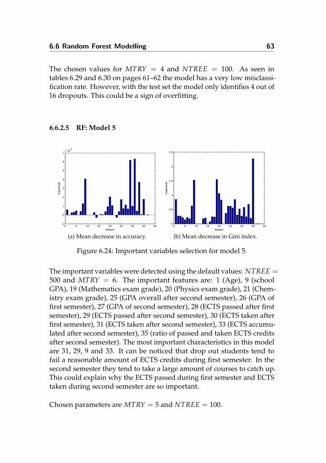
6.6 Random Forest Modelling 63
The chosen values for MTRY = 4 and NTREE = 100. As seen intables 6.29 and 6.30 on pages 61–62 the model has a very low misclassi-fication rate. However, with the test set the model only identifies 4 out of16 dropouts. This could be a sign of overfitting.
6.6.2.5 RF: Model 5
0 5 10 15 20 25 30 35 40-1
0
1
2
3
4
5
6
7x 10
-3
feature
mag
nitu
de
(a) Mean decrease in accuracy.
0 5 10 15 20 25 30 35 400
0.5
1
1.5
2
2.5
feature
mag
nitu
de
(b) Mean decrease in Gini index.
Figure 6.24: Important variables selection for model 5.
The important variables were detected using the default values: NTREE =500 and MTRY = 6. The important features are: 1 (Age), 9 (schoolGPA), 19 (Mathematics exam grade), 20 (Physics exam grade), 21 (Chem-istry exam grade), 25 (GPA overall after second semester), 26 (GPA offirst semester), 27 (GPA of second semester), 28 (ECTS passed after firstsemester), 29 (ECTS passed after second semester), 30 (ECTS taken afterfirst semester), 31 (ECTS taken after second semester), 33 (ECTS accumu-lated after second semester), 35 (ratio of passed and taken ECTS creditsafter second semester). The most important characteristics in this modelare 31, 29, 9 and 33. It can be noticed that drop out students tend tofail a reasonable amount of ECTS credits during first semester. In thesecond semester they tend to take a large amount of courses to catch up.This could explain why the ECTS passed during first semester and ECTStaken during second semester are so important.
Chosen parameters are MTRY = 5 and NTREE = 100.

64 Modelling
0 2 4 6 8 10 12 140
0.02
0.04
0.06
0.08
0.1
0.12
0.14
0.16
0.18
0.2
MTRY
Mea
n of
cla
ssifi
catio
ns
DDPD
(a) Mean of classsifications.
0 2 4 6 8 10 12 140
0.05
0.1
0.15
0.2
0.25
0.3
0.35
0.4
0.45
MTRY
Sta
ndar
d de
viat
ion
Cla
ssifi
catio
ns
DDPD
(b) Standard deviation of classsifica-tions.
Figure 6.25: Identification of MTY for model 5.
0 50 100 150 200 250 300 350 400 450 5000
0.5
1
1.5
2
2.5
NTREE
Mea
n of
cla
ssifi
catio
ns
DDPD
(a) Mean of classsifications.
0 50 100 150 200 250 300 350 400 450 5000
0.5
1
1.5
2
2.5
3
NTREE
Sta
ndar
d de
viat
ion
Cla
ssifi
catio
ns
DDPD
(b) Standard deviation of classsifica-tions.
Figure 6.26: Identification of NTREE, when MTRY = 5, for model 5.
DD DP PP PDTrain 9 0 331 0Test 0 4 91 0
Table 6.31: RF predictions using model 5.
Misclassification ratio 0.0092Drop out misclassification ratio 0.0092Drop out ratio in all misclassification 1
Table 6.32: Performance information of model 5.

6.6 Random Forest Modelling 65
The misclassification rates are very low, but it seems that model overfits.Model 5 do not identify any drop out students in the test set.
6.6.2.6 RF: Model 6
0 5 10 15 20 25 30 35 40 45-0.5
0
0.5
1
1.5
2
2.5x 10
-3
feature
mag
nitu
de
(a) Mean decrease in accuracy.
0 5 10 15 20 25 30 35 40 450
0.2
0.4
0.6
0.8
1
1.2
1.4
1.6
feature
mag
nitu
de
(b) Mean decrease in Gini index.
Figure 6.27: Important variables selection for model 6.
The important variables were detected using default values: NTREE =500 and MTRY = 6. The list of the important variables is very long.The important features are: 1 (Age), 6 (Mathematics and Technologyprogramme), 7 (Biotechnology programme), 8 (time after last schoolexam), 9 (school GPA), 19 (mathematics exam grade), 20 (physics examgrade), 21 (chemistry exam grade), 23 (gender:male), 24 - 26 (representsoverall GPA after fist-third semester), 27 (GPA of the first semester), 29(GPA of the third semester), 31-32 (represents ECTS passed during secondand third semester), 34-35 (represents ECTS taken during second andthird semester), 41 (ratio of passed and taken ECTS after third semester),44 (indicator that the student was more then 30 ECTS credits behindstudy plan). This large number of important variables makes it difficultto interpret the model. This could also be an indicator that the model isunreasonable.
Here MTRY = 6 and NTREE = 100. The model performance ratesconfirms that the model overfits. Probably, there were to little dropoutsthe in the training set to catch the structure.

66 Modelling
0 5 10 15 200
0.05
0.1
0.15
0.2
0.25
0.3
0.35
0.4
MTRY
Mea
n of
cla
ssifi
catio
ns
DDPD
(a) Mean of classsifications.
0 5 10 15 200
0.1
0.2
0.3
0.4
0.5
0.6
0.7
MTRY
Sta
ndar
d de
viat
ion
Cla
ssifi
catio
ns
DDPD
(b) Standard deviation of classsifica-tions.
Figure 6.28: Identification of MTY for model 6.
0 50 100 150 200 250 300 350 400 450 5000
0.1
0.2
0.3
0.4
0.5
0.6
0.7
0.8
0.9
1
NTREE
Mea
n of
cla
ssifi
catio
ns
DDPD
(a) Mean of classsifications.
0 50 100 150 200 250 300 350 400 450 5000
0.1
0.2
0.3
0.4
0.5
0.6
0.7
0.8
NTREE
Sta
ndar
d de
viat
ion
Cla
ssifi
catio
ns
DDPD
(b) Standard deviation of classsifica-tions.
Figure 6.29: Identification of NTREE, when MTRY = 5, for model 6.
DD DP PP PDTrain 8 0 333 0Test 1 3 91 0
Table 6.33: RF predictions using model 6.
Misclassification ratio 0.0069Drop out misclassification ratio 0.0069Drop out ratio in all misclassification 1
Table 6.34: Performance information of model 6.

6.6 Random Forest Modelling 67
6.6.2.7 RF: Model 7
0 10 20 30 40 50 60-4
-2
0
2
4
6
8
10
12x 10
-4
feature
mag
nitu
de
(a) Mean decrease in accuracy.
0 10 20 30 40 50 600
0.1
0.2
0.3
0.4
0.5
0.6
0.7
featurem
agni
tude
(b) Mean decrease in Gini index.
Figure 6.30: Important variables selection for model 7.
Default values: NTREE = 500 and MTRY = 7. As in model 6 the listof important features is long: 1 (age), 4 (Biomedicine programme), 5(Design and Innovation programme), 9 (school GPA), 13 (physic level A),14 (physic level B), 18 (chemistry level C), 19 (Mathematics exam grade),23 (gender:male), 25-27 (overall GPA of the second-fourth semester), 29-31 (semester GPA of second-fourth semester), 33 (passed ECTS duringsecond semester), 37 (takes ECTS during second semester), 39 (takesECTS during fourth semester), 41-42 (accumulated ECTS during second- third semester), 47 (ratio of passed and taken ECTS during fourthsemester).
DD DP PP PDTrain 12 0 332 0Test 0 1 91 0
Table 6.35: Model predictions using model 7.
Misclassification ratio 0.0023Drop out misclassification ratio 0.0023Drop out ratio in all misclassification 1
Table 6.36: Performance information of model 7.
Here MTRY = 6 and NTREE = 50. As in the previous model a large

68 Modelling
0 5 10 15 20 250
0.05
0.1
0.15
0.2
0.25
0.3
0.35
0.4
0.45
MTRY
Sta
ndar
d de
viat
ion
Cla
ssifi
catio
ns
DDPD
(a) Mean of classsifications.
0 5 10 15 20 250
0.02
0.04
0.06
0.08
0.1
0.12
0.14
0.16
0.18
0.2
MTRY
Mea
n of
cla
ssifi
catio
ns
DDPD
(b) Standard deviation of classsifica-tions.
Figure 6.31: Identification of MTY for model 7.
0 50 100 150 200 250 300 350 400 450 5000
0.1
0.2
0.3
0.4
0.5
0.6
0.7
0.8
0.9
1
NTREE
Mea
n of
cla
ssifi
catio
ns
DDPD
(a) Mean of classsifications.
0 50 100 150 200 250 300 350 400 450 5000
0.1
0.2
0.3
0.4
0.5
0.6
0.7
0.8
0.9
1
NTREE
Sta
ndar
d de
viat
ion
Cla
ssifi
catio
ns
DDPD
(b) Standard deviation of classsifica-tions.
Figure 6.32: Identification of NTREE, when MTRY = 5, for model 7.

6.6 Random Forest Modelling 69
number of important characteristics were found and the small amount ofdrop out students made the model useless.
6.6.2.8 RF: Model 8
0 10 20 30 40 50 60-1
-0.5
0
0.5
1
1.5
2
2.5
3
3.5x 10
-3
feature
mag
nitu
de
(a) Mean decrease in accuracy.
0 10 20 30 40 50 600
0.1
0.2
0.3
0.4
0.5
0.6
0.7
0.8
feature
mag
nitu
de
(b) Mean decrease in Gini index.
Figure 6.33: Important variables selection for model 8.
The important variables were detected using the default values: NTREE =500 and MTRY = 7. Important features selected: 1 (age), 9 (school GPA),13 (physics level A), 19 (mathematics exam grade), 20 (physics examgrade), 21 (chemistry exam level), 26-28 (overall GPA during third-fifthsemester), 31 (third semester GPA), 33 (fifth semester GPA), 34 (passedECTS during first semester), 39 (taken ECTS during first semester), 41(taken ECTS during third semester), 44-45 (accumulated ECTS duringfirst-second semester) and 47-48 (accumulated ECTS during fourth-fifthsemester).
DD DP PP PDTrain 7 0 332 0Test 0 3 90 0
Table 6.37: RF predictions using model 8.
Chosen values for MTRY = 6 and NTREE = 50. As in the previousmodel a large number of important characteristics were found and thesmall amount of drop out students made the model useless.

70 Modelling
0 2 4 6 8 10 12 14 16 180
0.02
0.04
0.06
0.08
0.1
0.12
0.14
0.16
0.18
0.2
MTRY
Mea
n of
cla
ssifi
catio
ns
DDPD
(a) Mean of classsifications.
0 2 4 6 8 10 12 14 16 180
0.05
0.1
0.15
0.2
0.25
0.3
0.35
0.4
0.45
MTRYS
tand
ard
devi
atio
n C
lass
ifica
tions
DDPD
(b) Standard deviation of classsifica-tions.
Figure 6.34: Identification of MTY for model 8.
0 50 100 150 200 250 300 350 400 450 5000
0.1
0.2
0.3
0.4
0.5
0.6
0.7
0.8
0.9
1
NTREE
Mea
n of
cla
ssifi
catio
ns
DDPD
(a) Mean of classsifications.
0 50 100 150 200 250 300 350 400 450 5000
0.1
0.2
0.3
0.4
0.5
0.6
0.7
0.8
0.9
1
NTREE
Sta
ndar
d de
viat
ion
Cla
ssifi
catio
ns
DDPD
(b) Standard deviation of classsifica-tions.
Figure 6.35: Identification of NTREE, when MTRY = 5, for model 8.
Misclassification ratio 0.0069Drop out misclassification ratio 0.0069Drop out ratio in all misclassification 1
Table 6.38: Performance information of model 8.

6.6 Random Forest Modelling 71
6.6.3 Final Model Using RF Technique
1 2 3 4 5 6 7 80
20
40
60
80
100
120
140
160
180
Models
Pre
dict
ed s
tude
nt to
dro
p ou
t
(a) Training
1 40
1
2
3
4
5
6
7
Models
Pre
dict
ed s
tude
nt to
dro
p ou
t
(b) Test
Figure 6.36: Final model determination using RF. Blue - classified dropout correctly, red - false alarms. The numbers are additional uniqueclassifications not previously classified by the lowered numbered models.
1 2 3 4 5 6 7 8 RateTrain correct 166 4 1 13 1 1 0 0 0.9394Train false 17 0 0 10 0 0 0 0 0.1268
Table 6.39: Important semester model selection for final RF model.
1 4 RateTest correct 7 0 0.3889Test false 7 0 0.5000
Table 6.40: Final RF model analysis.
For the training data the model gives a pre-drop out notice of 3.3871semester and for the test set 3.2857 semester in advance. No doubt thatwith training set model does excellent job. Just with the first model itidentifies around 84% of all dropouts with a 9% false alarm rate. However,the model validation results are very disappointing. The model willidentify around 39% of all dropouts with a high 50% false alarm rate.

72 Modelling
6.7 MARS Modelling
6.7.1 MARS Modelling Technique
MATLAB does not have an implemented MARS function. However, [13]has implemented MARS building and support functions:
• trainParams = aresparams(M, k-fold, cubic, [], mi, d) cre-ates a structure of MARS configuration parameter values.
– M maximal number of basis function in the forward-stepwisemethod.
– cubic if set to false a piecewise-linear polynomial is used.
– d in case of piecewise-linear polynomial is use then it can beset to the maximum allowed iterations.
– mi is the maximum degree of self interactions for the charac-teristics. This parameter is only used for the piecewise-linearpolynomial.
– k-fold number of folds to use in cross-validation.
• [model, time] = aresbuild(X, y, trainParams) is used to buildthe MARS models. X is the independent variable matrix, y is a vec-tor of the dependent variable and finally the parameters.
• Y = arespredict(model, X ) does prediction of the MARS modelwith the input X.
• [avgMSE, avgRMSE, avgRRMSE, avgR2] = arescv(X, Y, trainParams,
[], k) performs cross-validation. Options were used:
– trainParams model parameters.
– k number of folds.
This function results in the average mean squared error, averageroot mean squared error, average relative root mean squared error,average coefficient of determination and average execution time.

6.7 MARS Modelling 73
• eq = areseq(model, precision) gives the model in a mathemat-ical form. precision is the number of digits in the model coeffi-cients and knot sites.
As suggested in [5] the best way to choose M, d and mi is using cross-validation. The same paper mention the values of d and mi should befrom 1 to 3. The number of M depends on the number of characterist-ics in input matrix. The minimum number of characteristics is 23 (inapplication scoring model) and maximum 72 (in model 8 for the sixthsemester). The chosen interval for M was from 21 to 151 by a step of5 to save computational time. With every set of parameters arescv(X,Y, trainParams, [], k) computed which performed a 5 fold cross-validation. The parameters were selected by the lowest average meansquare error (avrMSE).
6.7.2 Overview of Individual MARS Semester Models
A description of the performance for each semester models can be seenin appendix C on page 111.
For all semester models no maximum interactions and number of self-interactions were chosen. The analysis showed that increasing these twoparameters would increase the mean square error variation, but remainsaround the same value. The maximum number and used number ofbasic functions in the final semester models vary from model to model.
As seen in fig. 6.37 on the next page MARS struggles when searching forthe best separation. For some semester models the required maximumnumber of basic functions can be quite high for the forward-stepwisemethod. The method reduces the number of basic functions but the finalmodel remains too complex carrying too many basic functions. In thefinal semester model, MARS will include the same characteristics severaltimes. This makes the model difficult to interpret.

74 Modelling
1 2 3 4 5 6 7 80
20
40
60
80
100
120
140
160
No. of models
Mai
mal
num
ber
of b
asic
func
tion
in th
e m
odel
(a) Maximum.
1 2 3 4 5 6 7 82
4
6
8
10
12
14
16
18
20
22
No. of models
Number of basic functions in the modelNumber of characteristics in the model
(b) Final.
Figure 6.37: Maximal number of basic functions in the forward-stepwiseprocess and number of basic functions in final semester model
6.7.3 Final Model Using MARS
1 2 3 4 5 6 7 80
10
20
30
40
50
60
Models
Pre
dict
ed s
tude
nt to
dro
p ou
t
(a) Training
1 40
1
2
3
4
5
6
Models
Pre
dict
ed s
tude
nt to
dro
p ou
t
(b) Test
Figure 6.38: Final model determination using MARS. Blue - classifieddrop out correctly, red - false alarms. The numbers are additional uniqueclassifications not previously classified by the lowered numbered models.
On the training set the model gives a pre-drop out notice of 2.7374semesters and on test set it is 2.4000 semesters in advance. In comparisonto the other models this is a bit lower. The model predicts around 50%of all dropouts, but the false alarm rate was observed at 37-59% in thetraining and test sets. Furthermore, the models are very complex canpose a challenge upon implementation.

6.7 MARS Modelling 75
1 2 3 4 5 6 7 8 RatioTrain correct 52 1 2 34 2 4 1 3 0.5000Train false 20 1 4 12 0 3 0 1 0.5973
Table 6.41: Important semester model selection for final MARS model.
1 4 RatioTest correct 5 5 0.5556Test false 6 0 0.3750
Table 6.42: Final MARS model analysis.

76 Modelling

CHAPTER 7
Result Analysis
7.1 Model Comparison
Model Number of models Correct class. False alarm TimeLogistic Regression 3 0.44 0.34 2.5CART 3 0.61 0.08 3CART Bagging 2 0.56 0.33 2.6Random forest 2 0.39 0.5 3.3MARS 2 0.56 0.38 2.4Current system - 0.33 0.80 2.5
Table 7.1: Model comparison table.
At the model building phase the most promising model was the randomforest. On the test set RF showed very low performance. This suggestthat RF overfitted. Logistic regression face problems with collinearity,that leads to low prediction rate with a high false alarm rate. MARS alsofails to predict drop out students correctly. As LR, MARS is also sensitiveto collinearity and noise.

78 Result Analysis
Most promising methods is CART. CART predicts 61% of all dropoutswith a false alarm rate of 8% based on 3 separate semester models. Itcan give the prediction of dropping out 3 semesters in advance beforestudent is actually going to drop out. Second best method is CARTbagging do it 2.6 semesters before and predicts 56% of all dropouts, butmisclassification rate is 33%. Both methods has similar prediction power,but to implement CART bagging would need a specific programs tohandle all the many trees generated while CART can be done with some’if’ conditions.
In comparison of current system to analysed methods, it performs worst.It identifies just 33% of dropouts with high false alarm rate 80%. Wherethe worst analysed model (LR) predicts 44% with false alarm rate 34%.This high rate of false alarm in the current student monitoring systemis because of two reasons. Fist, strong relation to the previous semester.If good student skipped one semester it most likely he or she will beidentified as a drop out for rest of the study time. Second, the long periodof student monitoring. If analysed models suggest to monitor studentsfor the first two or three semester, current system requires of studentsmonitoring during all study period.
7.2 Final CART Model Stability
CART showed very good performance on the training set and evensignificantly better on the test set. Further analysis of CART’s predictionstability will be done. The training set is divided in 9 folds of similar sizeas the test set. For each fold the final CART model will be applied.
As seen in fig. 7.1 on the facing page the drop out classification rate ismore or less stable around the correct average drop out rate of 53%. Thefalse alarm rate can vary from 8% to 45% with the average being 28%.
Figure 7.2 on the next page shows that model 1 is the strongest sourceof the false alarm. It can be due to a few reasons. First, in the firstmodel the chemistry grade is included. Chemistry is not very relevantfor the Mathematics and Technology programme. The model most likely

7.2 Final CART Model Stability 79
1 2 3 4 5 6 7 8 90.3
0.35
0.4
0.45
0.5
0.55
0.6
0.65
Fold number
Cor
ectly
cla
ssifi
ed d
rop
outs
(a) Drop out calssifications.
1 2 3 4 5 6 7 8 90.05
0.1
0.15
0.2
0.25
0.3
0.35
0.4
0.45
0.5
Fold number
Fal
se a
larm
rat
e
(b) False alarms rate.
Figure 7.1: CARTfinal model stability.
1 4 5-1
0
1
2
3
4
5
6
7
8
9
CART semester model
Mis
clas
sific
atio
n
Figure 7.2: CART individual semester models false alarm stability.
captured most of the dropouts from the Biomedicine programme wherechemistry is important. To avoid this all programmes with similar maintopics should be grouped and analysed separately. Another reason couldbe that students with low grades entering the university can graduate.The motivation is not included in the model and thus there can be somemisclassifications. It can be seen in fig. 7.2, that with time predictionsare more accurate. It is because, more information is known about thestudent capabilities.

80 Result Analysis
7.3 Important Variable Analysis
An additional task of this thesis was to identify the important factorscausing a student to drop out. This information can be obtained from themodels analyses. However, not all models are easily interpreted which isessentially the question here. The CART bagging model is a black boxmethod. This means the characteristics that are included in the model arenot really known. MARS provides information about the characteristicspicked up for during the model building, but the complexity of theMARS models complicates its interpretability and the importance forthe different characteristics is cluttered. Usually logistic regression canbe used for interpretation, yet only few of the coefficients were set tozero and due to the highly inter-correlated characteristics some of theestimates had large values and with opposite sign - also ruining theinterpretation.
CART does not provide an importance measure for the characteristicsin the model, but characteristics can be seen in a hierarchical order. Itcan become complicated if the tree is very large. The parent node isthe most important characteristic, but how does lower similar levelledcharacteristics rank relative to each other is not clear. Random Foresthas developed a characteristic measures. That is the mean decrease inaccuracy and mean decrease in Gini index. Important variables will becompared from CART and RF models.
Model 1: CART chooses mathematics and chemistry exam grades. RF choosesthe most significant characteristics: Design and Innovation pro-gramme and school GPA. However, mathematics and chemistryexam grades together with physics grade are also very significantin RF.
Model 4: CART an RF choose the first semester ratio of passed and takenECTS credits. It is worth to mention that school exam grades arealso significantly important.
Model 5: CART chooses the ratio of passed and taken ECTS credits after thesecond semester. RF does not consider this characteristic equally

7.3 Important Variable Analysis 81
important although it is in the list of the four most important char-acteristics. The school exam grades are still important.
Model 6: CART chooses the ratio of passed and taken ECTS credits afterthe third semester. This characteristics was also one of the mostimportant in RF. Furthermore, RF chooses the individual character-istics passed and taken ECTS credits during the second and thirdsemester.
Model 8: CART chooses the accumulated ECTS credits after the third semester.RF also refers to the third semester, but to the GPA of the semester.RF gives additionally a lot of importance to the school exam grades.
From this comparison it can be seen that there is no doubt that the schoolexam grades are very important while the GPA is not too important.A high school GPA can be driven by subjects irrelevant to the DTUstudy programmes thus not necessarily provide any useful information.The three specific school exam results are a good representation for thestudents readiness for a technical university.
When a student reaches university, the best performance indicators arepassed and taken ECTS credits per semester. Depending on the model itmight also include the ratio of the passed and taken ECTS credits. CARTuses the ratio, while RF the individual characteristics.
From this summary it can be concluded that the current dropout detectionsystem is not optimal for DTU. The being behind by 30 credits indicatorwas only included in one last semester RF model and it was only mediumimportant. This measure might be worth to check when the study timegets long.

82 Result Analysis

CHAPTER 8
Conclusion
High rates of dropouts every year that cost a lot of money for the taxpayers is forcing universities to search for new solutions. The current sys-tem suggests to offer consultation to a student who is behind by 30 ECTScredits or more. This master’s thesis offers a different approach for dropout students detection. The new method suggest to keep track on studentperformance using their application and performance information overseveral semesters. Before the student even starts their studies the modelwill evaluate whether the student will drop out. After every semester thestudent’s performance must be checked by model to make sure that thestudent is still performing good enough to graduate. Though some ofthe drop out student can not be identified due to their high performancerates, most often these students decide to leave university for personalreasons.
Six techniques were compared for every semester status identification:logistic regression (LR), principle component logistic regression (PC-LR),classification and regression trees (CART), classification and regressiontree bagging (CART bagging), random forest (RF) and multivariate adapt-ive regression splines (MARS). After testing each model it was concluded

84 Conclusion
that LR failed to perform due to hight collinearity among the variables.Principle components analysis do not improve the performance of logisticregression. RF overfits the data which results in many misclassifications,though some of the literature suggests random forest cannot overfit dueto its model building technique. MARS also failed to correctly predictdrop out students. The most efficient models were build by CART andCART bagging methods. These methods could identify more than half ofthe drop out students with low false alarm rates. These methods showedthat it is enough to keep track on students’ performance for no morethan the first three semesters. CART can be perform on any programsupporting logic functions, but for the CART bagging it is necessary toadopt a special program.
Methods like CART and RF gave an understanding of the indicatorscausing the students to drop outs. It was identified that chemistry, math-ematics and physics exam grades are significant indicators for a student’sability to continue. Surprisingly, school GPA was just a medium signi-ficance indicator. One of the most important performance characteristicwas the ratio of passed and taken ECTS credits per semester. CART chosethis ratio as a main indicator for three semester models. The indicatorthat student is behind by 30 ECTS credits or more was chosen once byone of the by RF for later semester models. This leads to the conclusion,that current system is not optimal for DTU.
The current student monitoring system is not better then other analysedmethods. The 30 ECTS credit delay indicator makes more confusion thenhelps to identify drop out students. It do not show how well performsthe student and student‘s capabilities. It indicates whether the studentmissed one or more semester. That has low relation to the student status.What is more, using this system student must be monitored for all studyperiod, while with suggested methods students must be monitored justfor few semesters.
The further analysis and implementation of this new system will allowDTU identify drop out students early on. This would give enough timefor the university to intervene and help those troubled students. As morestudents actually graduates the university will be paid by the state andwill help the government to achieve the national goal that half of the

8.1 Future Work 85
young people should have the higher education.
8.1 Future Work
In the future three aspects of this topic should be investigated. First,models for groups of programmes. Second, categorization of drop outand passed students. Third, information about student performance inmandatory courses.
It has been demonstrated that the chemistry grade is chosen by manymodels. However, this subject does not seem all too relevant for Designand Innovation or Mathematics and Technology programmes. Chemistrywas likely chosen because there are so many dropouts in the Biomedicineand Biotechnology programmes where a good chemistry exam gradeseem more important. It should be investigated if specific programmesrequire a specific school exam. For example, the Biomedicine and Bio-technology programmes’ main exam would be chemistry while Physicsand Mechanics would be physics.
Another aspect that should be investigated is categorization of the stu-dents. As demonstrated in the data analysis the data is very noisy. Goodstudents drop out and bad students graduate. A suggestion could be togroup students into four groups. Two groups for pass students: passedat a high performance level, passed at a low performance level and twogroups for dropouts: drop out at a high performance level and dropout at a low performance level. Students who drop out at the high per-formance level would be a student quitting due to personal reasons andthis group is likely impossible to detect. The highest attention shouldbe given to the group that drop out at the low performance level. Thisgroup consists of students lacking motivation and social establishment.Students who passed at the low performance level would be studentseither solely interested in graduating but not in the studies itself or hav-ing troubles with studying. For the model to perform better a studentcategorization should be examined. Their motivation, interest in the sub-ject and their evaluation of the university should give an understandingof the group boundaries.

86 Conclusion
At DTU the students have freedom to choose their courses. Some of thecourses are easier than others, yet there are some mandatory courses thatmust be completed during the programme. Investigating the mandatorycourses should give an equal comparison among the students in theprogram.
Changing the study programme within DTU can be considered droppingout of the first programme. [14] suggests student who dropped outonce are likely to drop out again. The effect of jumping between theprogrammes should be investigated.

Abbreviations
avgRRMSE average of relative root mean squared error.
avrMSE average of means square error.
avgR2 average of R-square measure.
avrRMSE average of root square error.
CART Classification and Regression Trees
d maximal number of allowed interactions in MARS modelling.
DD group of students who drop out and were classified as dropouts.
DP group of students who drop out but were classified as pass stu-dents.
ECTS A Accumulated ECTS credits
ECTS L Indicator if 30 ECTS credits behind
ECTS P ECTS credits passed
ECTS R ratio of passed and taken ECTS credits
ECTS T ECTS credits taken
GCV generalized cross-validation.

88 Conclusion
GPA O overall grade point average
GPA S semester grade point average
LR Logistic Regression
M maximal number of basic functions in forward-stepwise method ofMARS modelling.
MARS Multivariate Adaptive Regression Splines.
MDA mean decrease in accuracy measure.
MDG mean decrease in Gini index measure.
mi maximal number of allowed self interactions.
MTRY the smallest number of variables rampantly selected in the randomforest method.
NTREE number of tree is random forest method.
OOB error out-of-bag error.
PD group of students who passed but were classified as dropouts.
PP group of students who passed and were classified as passed stu-dents.
PC-LR Principle Component Logistic Regression.
RF Random Forest

APPENDIX A
LR Models for Every Semester
A.1 LR: Model 1
Interaction Age Lock stud. In. stud.β -4116.9220 0.1160 -0.5950 0
Tech. biomed. stud. Design stud. Mat stud. Biotech. stud.β 0.1270 -1.0650 0.1800 -0.0930
Time af. exam GPA Math lev. A Math lev. Bβ -0.1240 -0.0550 -20.8000 0
Math lev. C Physics lev. A Physics lev. B Physics lev. Cβ 0.0000 256204.7870 256204.8680 14.7730
Chemistry lev. A Chemistry lev. B Chemistry lev. C Math gradeβ -252063.55900 -252063.6090 252063.6090 -0.1210
Physics grade Chemistry grade Man Womanβ -0.2090 -0.2440 0 -0.2200
Table A.1: Coefficient of logistic regression model 1.
Reasonable coefficient estimated for some characteristics can be noted.

90 LR Models for Every Semester
Students who had mathematics at A level is less likely to drop out. Itseems that physics and chemistry exam grades are more significant thanmathematics exam grade. This can be due to the large data set fromthe Biomedicine and Biotechnology programmes. Females and studentsfrom the Design and Innovation programme have a lower drop out rate.
DD DP PP PDTrain 39 109 329 15Test 15 25 82 4
Table A.2: Predictions using the model table A.1 on the preceding page
Misclassification ratio 0.2476Drop out misclassification ratio 0.2168Drop out ratio in all misclassification 0.8758Not classified 30
Table A.3: Performance information for model table A.1 on thepreceding page
Table A.3 shows some 87% of the misclassifications are uncaught dropout students.
A.2 LR: Model 2
Table A.4 on the facing page has almost the same important character-istics as table A.1 on the previous page. The greatest difference is thechemistry level coefficients. Table A.6 on the facing page shows thismodel has a low false alarm rate of 0.0936. However the model did notidentify 45 out of 51 drop out students.

A.3 LR: Model 3 91
Interaction Age Lock stud. In. stud.β -143.7010 0.0650 -10.3280 -27.5760
Tech. biomed. stud. Design stud. Mat stud. Biotech. stud.β -2.2520 -4.5490 -2.2140 -3.2530
Time af. exam GPA Math lev. A Math lev. Bβ 0.0680 -0.1480 1909.1380 -10.0420
Math lev. C Physics lev. A Physics lev. B Physics lev. Cβ 0 -1730.2700 -1729.4840 9.7300
Chemistry lev. A Chemistry lev. B Chemistry lev. C Math gradeβ -17.7220 -17.5100 -17.0290 -0.2290
Physics grade Chemistry grade Man Womanβ -0.1840 -0.3660 0 -0.2200
Table A.4: Coefficients for the logistic regression model 2
DD DP PP PDTrain 5 35 342 1Test 1 10 85 2
Table A.5: Predictions using model table A.4
Misclassification ratio 0.0998Drop out misclassification ratio 0.0936Drop out ratio in all misclassification 0.9375Not classified 23
Table A.6: Performance information for model table A.4
A.3 LR: Model 3
The model coefficients in table A.7 on the next page look more reasonable.However, as in earlier model there were warnings during the estimation.Still this model has low performance abilities.

92 LR Models for Every Semester
Interaction Age Lock stud. In. stud.β -145.8170 0.0260 117.1710 -12.2550
Tech. biomed. stud. Design stud. Mat stud. Biotech. stud.β -36.5070 -38.6520 -36.1480 -37.3460
Time af. exam GPA Math lev. A Math lev. Bβ 0.1000 -0.1950 74.3710 0
Math lev. C Physics lev. A Physics lev. B Physics lev. Cβ 0 39.1270 39.7740 0.0000
Chemistry lev. A Chemistry lev. B Chemistry lev. C Math gradeβ -41.4560 -41.6390 -41.2480 -0.2380
Physics grade Chemistry grade Man Womanβ -0.02200 -0.5850 0 -0.2200
Table A.7: Coefficient of logistic regression model 3.
DD DP PP PDTrain 5 28 342 2Test 1 8 85 1
Table A.8: Predictions using model table A.7
Misclassification ratio 0.0826Drop out misclassification ration 0.0763Drop out ration in all misclassification 0.9231Not classified 22
Table A.9: Model table A.7 performance information.
A.4 LR: Model 4
It can be noted in table A.10 on the facing page that the ratio of takenand passed ECTS credits is most significant among the performancecharacteristics from the first semester. Table A.11 on the next pageshows the overall training prediction performance is much better thanthe test performance. It is most likely that the model did not catch theunderling structure.

A.5 LR: Model 5 93
Interaction Age Lock stud. In. stud.β -28.6370 0.1280 159.4340 0
Tech. biomed. stud. Design stud. Mat stud. Biotech. stud.β -51.9410 -54.7600 -54.2770 -53.2230
Time af. exam GPA Math lev. A Math lev. Bβ -0.2460 -0.3780 0 0
Math lev. C Physics lev. A Physics lev. B Physics lev. Cβ 0 -37.4600 -37.3960 0
Chemistry lev. A Chemistry lev. B Chemistry lev. C Math gradeβ -39.2180 -39.3280 -38.2030 -0.0530
Physics grade Chemistry grade Man Womanβ 0.4620 -0.5680 0.0000 -0.2200
GPA O 1 GPA S 1 ECTS P 1 ECTS T 1β 0.1950 0.1270 -0.3260 0.5130
ECTS A 1 ECTS R 1 ECTS L 1β -0.2500 -1.9980 0.0000
Table A.10: Coefficients for the logistic regression model 4.
DD DP PP PDTrain 19 25 335 3Test 1 11 84 1
Table A.11: Predictions using model table A.1 on page 89
Misclassification ratio 0.0835Drop out misclassification ration 0.0752Drop out ration in all misclassification 0.9000Not classified 49
Table A.12: Performance information for model table A.10
A.5 LR: Model 5
From table A.13 on the following page it is difficult to interpret the result.For example the GPA overall after the second semester and GPA ofsecond semester are highly correlated due to their nature. For this reason,

94 LR Models for Every Semester
Interaction Age Lock stud. In. stud.β 58.7380 26.9000 -93.2100 197.8790
Tech. biomed. stud. Design stud. Mat stud. Biotech. stud.β -136.2840 -292.6380 -169.8330 -142.1090
Time af. exam GPA Math lev. A Math lev. Bβ -82.3460 105.6830 1113.2170 0.0000
Math lev. C Physics lev. A Physics lev. B Physics lev. Cβ 0.0000 -107.7690 -47.3640 0.0000
Chemistry lev. A Chemistry lev. B Chemistry lev. C Math gradeβ 245.3770 600.1370 746.9250 -117.5030
Physics grade Chemistry grade Man Womanβ -61.6550 -44.8300 0.0000 64.5770
GPA O 1 GPA O 2 GPA S 1 GPA S 2β 44.3950 -124.4460 0.2770 103.3640
ECTS P 1 ECTS P 2 ECTS T 1 ECTS T 2β 13.7160 -52.1930 -50.5980 19.4430
ECTS A 1 ECTS A 2 ECTS R 1 ECTS R 2β 0.0000 32.4580 -1969.5560 739.8820
ECTS L 1 ECTS L 2β 0.0000 -506.2760
Table A.13: Coefficients for the logistic regression model 5.
these two variables have high coefficient values but with opposite sign.
DD DP PP PDTrain 4 3 332 1Test 0 3 81 6
Table A.14: Predictions using model fig. 6.6 on page 47
Although this model does have a low misclassification ratio it has a lowprediction power.

A.5 LR: Model 5 95
Misclassification ratio 0.0302Drop out misclassification ratio 0.0140Drop out ratio in all misclassification 0.4615Not classified 39
Table A.15: Performance information for model table A.13 on the facingpage.

96 LR Models for Every Semester
A.6 LR: Model 6
Interaction Age Lock stud. In. stud.β 48.7210 -22.1190 -286.8410 -203.7010
Tech. biomed. stud. Design stud. Mat stud. Biotech. stud.β 17.1800 -24.4050 60.3770 40.1240
Time af. exam GPA Math lev. A Math lev. Bβ 18.4890 11.5320 -35.8910 0.0000
Math lev. C Physics lev. A Physics lev. B Physics lev. Cβ 0.0000 -112.1210 -98.6510 21.8890
Chemistry lev. A Chemistry lev. B Chemistry lev. C Math gradeβ 238.8280 110.3730 201.7730 6.6740
Physics grade Chemistry grade Man Womanβ 13.0800 -18.4750 0.0000 24.9890
GPA O 1 GPA O 2 GPA O 3 GPA S 1β 7.3370 28.6440 -10.0800 6.3800
GPA S 2 GPA S 3 ECTS P 1 ECTS P 2β -17.5730 -7.7710 -35.5390 -50.3550
ECTS P 3 ECTS T 1 ECTS T 2 ECTS T 3β -1.0820 26.7230 -2.6470 15.9420
ECTS A 1 ECTS A 2 ECTS A 3 ECTS R 1β -36.9050 64.0060 -18.9740 301.8250
ECTS R 2 ECTS R 3 ECTS L 1 ECTS L 2β 27.4430 313.6580 0.0000 -104.3470
ECTS L 3β 13.2090
Table A.16: Coefficients for the logistic regression model 6.
DD DP PP PDTrain 6 1 335 0Test 1 3 85 0
Table A.17: Predictions using model fig. 6.6 on page 47
Table A.16 shows that this model has the same problems as the previousmodels. However, it can be seen that the model emphasizes the ratio ofpassed and taken ECTS credits during first semesters.

A.7 LR: Model 7 97
Misclassification ratio 0.0093Drop out misclassification ratio 0.0093Drop out ratio in all misclassification 1Not classified 37
Table A.18: Performance information for model table A.16 on the facingpage.
A.7 LR: Model 7
DD DP PP PDTrain 2 0 335 0Test 0 1 83 0
Table A.19: Predictions using model table A.21 on the next page
Misclassification ratio 0.0024Drop out misclassification ratio 0.0024Drop out ratio in all misclassification 1Not classified 35
Table A.20: Performance information for model table A.21 on the nextpage.
Table A.19 shows that model identified correctly all pass students. Thesame plot shows that model correctly classified dropouts in training setwhile in test it missed. This is due to small dropouts number in thetraining set.

98 LR Models for Every Semester
Interaction Age Lock stud. In. stud.β -52.6730 -4.7950 -48.6170 -58.9840
Tech. biomed. stud. Design stud. Mat stud. Biotech. stud.β 0.0000 16.4000 50.0270 61.7250
Time af. exam GPA Math lev. A Math lev. Bβ 4.0500 -18.8170 -13.5530 0.0000
Math lev. C Physics lev. A Physics lev. B Physics lev. Cβ 0.0000 -31.5970 -39.2630 0.0000
Chemistry lev. A Chemistry lev. B Chemistry lev. C Math gradeβ -117.9800 -110.4200 -117.7010 5.1410
Physics grade Chemistry grade Man Womanβ -11.5560 19.7970 0.0000 1.1530
GPA O 1 GPA O 2 GPA O 3 GPA O 4β -12.4990 52.7470 -6.9470 -36.0350
GPA S 1 GPA S 2 GPA S 3 GPA S 4β 0.0000 -15.9480 11.3880 8.8080
ECTS P 1 ECTS P 2 ECTS P 3 ECTS P 4β -2.6940 -1.1360 -5.5330 -14.9100
ECTS T 1 ECTS T 2 ECTS T 3 ECTS T 4β 2.9500 1.4370 -4.1140 5.2410
ECTS A 1 ECTS A 2 ECTS A 3 ECTS A 4β 0.0000 -13.7760 4.8270 7.7260
ECTS R 1 ECTS R 2 ECTS R 3 ECTS R 4β 85.0670 151.5130 -125.7120 136.5570
ECTS L 1 ECTS L 2 ECTS L 3 ECTS L 4β 0.0000 -103.8210 97.0010 -6.7590
Table A.21: Coefficients for the logistic regression model 7.

A.8 LR: Model 8 99
A.8 LR: Model 8
Interaction Age Lock stud. In. stud.β 191.6930 5.8580 149.1860 0.0000
Tech. biomed. stud. Design stud. Mat stud. Biotech. stud.β 0.0000 287.4420 186.7700 249.5920
Time af. exam GPA Math lev. A Math lev. Bβ -20.6310 -13.5890 3.6590 0.0000
Math lev. C Physics lev. A Physics lev. B Physics lev. Cβ 0.0000 43.7140 -18.2440 23.5720
Chemistry lev. A Chemistry lev. B Chemistry lev. C Math gradeβ 110.8750 67.6620 83.8060 -6.5800
Physics grade Chemistry grade Man Womanβ 4.8570 -21.6060 0.0000 -26.0750
GPA O 1 GPA O 2 GPA O 3 GPA O 4β 4.3560 8.4510 -33.3630 -14.4330
GPA O 5 GPA S 1 GPA S 2 GPA S 3β 42.4270 3.3510 5.8460 7.2700
GPA S 4 GPA S 5 ECTS P 1 ECTS P 2β 1.1100 -7.9150 -13.2290 -28.7930
ECTS P 3 ECTS P 4 ECTS P 5 ECTS T 1β -79.8320 13.8150 2.6010 -18.1430
ECTS T 2 ECTS T 3 ECTS T 4 ECTS T 5β -15.2690 18.4880 2.2630 -6.3680
ECTS A 1 ECTS A 2 ECTS A 3 ECTS A 4β -15.8120 -8.2510 71.2860 -18.2060
ECTS A 5 ECTS R 1 ECTS R 2 ECTS R 3β 2.8250 -269.2820 -668.8170 354.6240
ECTS R 4 ECTS R 5 ECTS L 1 ECTS L 2β 128.7720 -218.6120 0.0000 148.5470
ECTS L 3 ECTS L 4 ECTS L 5β -12.5840 -96.0870 63.1400
Table A.22: Coefficients for the logistic regression model 8.
The sixth semester model is no different from the previous models. Itfaces the same problems: warning during model estimation and some

100 LR Models for Every Semester
DD DP PP PDTrain 6 0 333 0Test 0 3 80 2
Table A.23: Predictions using model table A.22 on the preceding page
Misclassification ratio 0.0118Drop out misclassification ratio 0.0071Drop out ratio in all misclassification 0.6000Not classified 36
Table A.24: Performance information model table A.22 on the precedingpage.
of coefficients have very high estimates. Also there are only a few coeffi-cients set to zero, which makes the model difficult to interpret.

APPENDIX B
CART Bagging Models forEvery Semester
B.1 CART Bagging: Model 1
0 100 200 300 400 5000.27
0.28
0.29
0.3
0.31
0.32
0.33
0.34
0.35
0.36
Number of grown trees
Men
a of
out
-of-
bag
clas
sific
atio
n er
ror
(a) Mean.
0 100 200 300 400 5000
0.005
0.01
0.015
0.02
0.025
0.03
Number of grown trees
Sta
ndar
t dev
iatio
n of
out
-of-
bag
clas
sific
atio
n er
ror
(b) Standard deviation.
Figure B.1: Identification of the number trees required for model 1 usingout-of-bag error of five models.
Figure B.1 shows the mean stabilizes around 200 trees, but the standard

102 CART Bagging Models for Every Semester
deviation only around 300. It is also important to note, that even using alarge number of trees the out-of-bag error is high.
DD DP PP PDTrain 149 8 359 0Test 8 33 85 6
Table B.1: Predictions using model fig. B.1 on the previous page
Misclassification ratio 0.0735Drop out misclassification ratio 0.0633Drop out ratio in all misclassification 0.8723Chosen number of trees 300
Table B.2: Performance information on model fig. B.1 on the previouspage.
Table B.2 shows that the model performance on the training data is verygood. However with the test set it is poor. This could be an indication,that the method overfits.
B.2 CART Bagging: Model 2
0 100 200 300 400 5000.02
0.025
0.03
0.035
0.04
0.045
Number of grown trees
Men
a of
out
-of-
bag
clas
sific
atio
n er
ror
(a) Mean.
0 100 200 300 400 5000
0.002
0.004
0.006
0.008
0.01
0.012
0.014
0.016
Number of grown trees
Sta
ndar
t dev
iatio
n of
out
-of-
bag
clas
sific
atio
n er
ror
(b) Standard deviation.
Figure B.2: Identification of the number trees required for model 2 usingout-of-bag error of five models.

B.3 CART Bagging: Model 3 103
It is seen in fig. B.2 on the preceding page that the mean and standarddeviation of the out-of-bag error stabilises when there are more than 40trees in the model.
DD DP PP PDTrain 4 4 359 0Test 0 2 91 0
Table B.3: Predictions using model fig. B.2 on the preceding page
Misclassification ratio 0.0130Drop out misclassification ratio 0.0130Drop out ratio in all misclassification 1Chosen number of trees 40
Table B.4: Performance information on model fig. B.2 on the precedingpage.
As in model 1, model 2 is also overfitting. For the training set the modelperforms decent, but it fails to predict the dropouts in the test set.
B.3 CART Bagging: Model 3
0 100 200 300 400 500
0.08
0.09
0.1
0.11
0.12
0.13
0.14
Number of grown trees
Men
a of
out
-of-
bag
clas
sific
atio
n er
ror
(a) Mean.
0 100 200 300 400 5000
0.002
0.004
0.006
0.008
0.01
0.012
0.014
0.016
0.018
Number of grown trees
Sta
ndar
t dev
iatio
n of
out
-of-
bag
clas
sific
atio
n er
ror
(b) Standart deviation.
Figure B.3: Identification of the number trees required for model 3 usingout-of-bag error of five models..

104 CART Bagging Models for Every Semester
DD DP PP PDTrain 33 2 359 0Test 1 8 91 1
Table B.5: Predictions using model fig. B.3 on the previous page
Misclassification ratio 0.0202Drop out misclassification ratio 0.0202Drop out ratio in all misclassification 1Chosen number of trees 300
Table B.6: Performance information on model fig. B.3 on the previouspage.
The mean stabilizes in fig. B.3a on the preceding page between 250 and300 trees. The standard deviation became almost constant after 300 trees.This model is also overfitting.
B.4 CART Bagging: Model 4
0 100 200 300 400 5000.09
0.1
0.11
0.12
0.13
0.14
0.15
0.16
0.17
0.18
0.19
Number of grown trees
Men
a of
out
-of-
bag
clas
sific
atio
n er
ror
(a) Mean.
0 100 200 300 400 5000
0.005
0.01
0.015
0.02
0.025
Number of grown trees
Sta
ndar
t dev
iatio
n of
out
-of-
bag
clas
sific
atio
n er
ror
(b) Standard deviation.
Figure B.4: Identification of the number trees required for model 4 usingout-of-bag error of five models.
Model 4 performs well on the training set. It do not identify 3 dropouts.Yet on the test set it do not identify 14 dropouts.

B.5 CART Bagging: Model 5 105
DD DP PP PDTrain 59 3 359 0Test 2 14 89 2
Table B.7: Predictions using model fig. B.4 on the facing page
Misclassification ratio 0.0360Drop out misclassification ratio 0.03022Drop out ratio in all misclassification 0.8947Chosen number of trees 150
Table B.8: Performance information on model fig. B.4 on the facing page.
B.5 CART Bagging: Model 5
0 100 200 300 400 500
0.04
0.045
0.05
0.055
0.06
0.065
0.07
Number of grown trees
Men
a of
out
-of-
bag
clas
sific
atio
n er
ror
(a) Mean.
0 100 200 300 400 5000
0.001
0.002
0.003
0.004
0.005
0.006
0.007
0.008
0.009
0.01
Number of grown trees
Sta
ndar
t dev
iatio
n of
out
-of-
bag
clas
sific
atio
n er
ror
(b) Standard deviation.
Figure B.5: Identification of the number trees required for model 5 usingout-of-bag error of five models..
Model stabilises with 100 trees.
From table B.10 on the next page it is seen that model 5 performs wellwith the training set. It identifies 93% of all dropouts. On the test set themodel identifies only 50% of the dropouts, but raises no false alarms.

106 CART Bagging Models for Every Semester
DD DP PP PDTrain 13 2 359 0Test 2 2 91 0
Table B.9: Predictions using model fig. B.5 on the preceding page
Misclassification ratio 0.0085Drop out misclassification ratio 0.0085Drop out ratio in all misclassification 1Chosen number of trees 100
Table B.10: Performance information on model fig. B.5 on the precedingpage.
B.6 CART Bagging: Model 6
0 100 200 300 400 500
0.04
0.045
0.05
0.055
0.06
0.065
Number of grown trees
Men
a of
out
-of-
bag
clas
sific
atio
n er
ror
(a) Mean.
0 100 200 300 400 5000
0.002
0.004
0.006
0.008
0.01
0.012
Number of grown trees
Sta
ndar
t dev
iatio
n of
out
-of-
bag
clas
sific
atio
n er
ror
(b) Standard deviation.
Figure B.6: Identification of the number trees required for model 6 usingout-of-bag error of five models.
Both the mean and standard deviation stabilizes around 100 trees. As theprevious models, this model performs well on the training set, but failson the test set. It identified 12 out of 14 dropouts, with no false alarms onthe training data set while on the test set it did not identify any dropouts.

B.7 CART Bagging: Model 7 107
DD DP PP PDTrain 12 2 359 0Test 0 4 91 0
Table B.11: Predictions using model fig. B.6 on the preceding page
Misclassification ratio 0.0128Drop out misclassification ration 0.0128Drop out ration in all misclassification 1Chosen number of trees 100
Table B.12: Performance information on model fig. B.6 on the precedingpage.
B.7 CART Bagging: Model 7
0 100 200 300 400 5000.012
0.014
0.016
0.018
0.02
0.022
0.024
Number of grown trees
Men
a of
out
−of
−ba
g cl
assi
ficat
ion
erro
r
(a) Mean.
0 100 200 300 400 5000
0.002
0.004
0.006
0.008
0.01
0.012
Number of grown trees
Sta
ndar
t dev
iatio
n of
out
−of
−ba
g cl
assi
ficat
ion
erro
r
(b) Standard deviation.
Figure B.7: Identification of the number trees required for model 7 usingout-of-bag error of five models.
The model well identified pass students, but fails to identify dropouts.Most likely it is due to the small ratio of drop out students in the trainingset. There were only 5 dropouts in the training set.

108 CART Bagging Models for Every Semester
DD DP PP PDTrain 3 2 359 0Test 0 1 91 0
Table B.13: Predictions using model fig. B.7 on the previous page
Misclassification ratio 0.0066Drop out misclassification ration 0.0066Drop out ration in all misclassification 1Chosen number of trees 50
Table B.14: Performance on model fig. B.7 on the previous page.
B.8 CART Bagging: Model 8
The out-of-bag error is constant in mean and standard deviation aftersome 150 trees. Table B.15 identifies all drop out and pass student intraining set, but fails to identify the dropouts in the test set. As in theprevious models it is due to the small number of dropouts (12) so themodel overfits.
DD DP PP PDTrain 12 0 355 0Test 0 3 90 0
Table B.15: Predictions using model fig. B.8 on the next page

B.8 CART Bagging: Model 8 109
Misclassification ratio 0.0065Drop out misclassification ratio 0.0065Drop out ratio in all misclassification 1Chosen number of trees 150
Table B.16: Performance information on model fig. B.8.
0 100 200 300 400 5000.03
0.035
0.04
0.045
0.05
0.055
0.06
0.065
0.07
0.075
Number of grown trees
Men
a of
out
-of-
bag
clas
sific
atio
n er
ror
(a) Mean.
0 100 200 300 400 5000
0.002
0.004
0.006
0.008
0.01
0.012
0.014
0.016
0.018
Number of grown trees
Sta
ndar
t dev
iatio
n of
out
-of-
bag
clas
sific
atio
n er
ror
(b) Standard deviation.
Figure B.8: Identification of the number trees required for model 8 usingout-of-bag error of five models.

110 CART Bagging Models for Every Semester

APPENDIX C
MARS Models for EverySemester
C.1 MARS: Model 1
050
100150
200
1
2
30
0.2
0.4
0.6
0.8
1
1.2
1.4
Mmi
MS
E
(a) Parameters mi and M.
050
100150
200
1
2
30
0.2
0.4
0.6
0.8
1
1.2
1.4
Md
MS
E
(b) Parameters d and M.
Figure C.1: Variable identification for model 1.

112 MARS Models for Every Semester
BF1 = max(0, 0.34232− school GPA)
BF2 = max(0, Design and Innovation programme + 0.70027)BF3 = max(0, chemistry exam grade− 1.9528)BF4 = max(0, physics exam grade− 0.67752)BF5 = max(0, physics exam grade− 0.90619)BF6 = max(0, chemistry exam grade− 0.91098)BF7 = max(0, chemistry exam grade− 1.1194)BF8 = max(0,−0.46585− physics exam grade)
y = 0.31632 + 0.082916 · BF1− 0.099606 · BF2 (C.1)− 2.2102 · BF3− 1.034 · BF4 + 1.5881 · BF5− 1.2418 · BF6 + 1.9649 · BF7 + 0.13511 · BF8
DD DP PP PDTrain 48 109 336 13Test 4 37 85 6
Table C.1: Predictions using model eq. (C.1)
Misclassification ratio 0.2546Drop out misclassification ratio 0.2253Drop out ratio in all misclassification 0.8848
Table C.2: Model eq. (C.1) performance information.
As seen in fig. C.1 on the previous page the mean square error is almostconstant for all combinations of d, mi and M. However increasing d or midoes increase the variation of the error. The optimal values are M = 151,mi = 1 and d = 1. As in many of the previous models the most importantcharacteristics are exam grades, school GPA and Design and Innovationprogramme. Unfortunately the model performances is very poorly.

C.2 MARS: Model 2 113
050
100150
200
1
2
30
200
400
600
800
1000
1200
1400
Mmi
MS
E
(a) Parameters mi and M.
050
100150
200
1
2
30
200
400
600
800
1000
1200
1400
Md
MS
E
(b) Parameters d and M.
Figure C.2: Variable identification for model 2.
C.2 MARS: Model 2
BF1 = max(0, mathematics exam grade + 1.9441)BF2 = max(0, mathematics exam grade + 1.5453)BF3 = max(0,−1.1797− physical exam grade)
y = 0.27218− 0.60897 · BF1 + 0.63589 · BF2 + 0.20369 · BF3 (C.2)
DD DP PP PDTrain 4 39 358 1Test 0 11 91 2
Table C.3: Predictions using model eq. (C.2)
Misclassification ratio 0.1012Drop out misclassification ratio 0.0992Drop out ratio in all misclassification 0.9804
Table C.4: Model eq. (C.2) performance information.
The optimal values were chosen to M = 140, mi = 1 and d = 1. Most ofthe analysed methods failed to build model 2. MARS is no exception.

114 MARS Models for Every Semester
C.3 MARS: Model 3
050
100150
200
1
2
30
500
1000
1500
2000
2500
3000
Mmi
MS
E
(a) Parameters mi and M.
050
100150
200
1
2
30
500
1000
1500
2000
2500
3000
Md
MS
E
(b) Parameters d and M.
Figure C.3: Variable identification for model 3.
BF1 = max(0, physics exam grade + 1.0746)BF2 = max(0, mathematics exam grade + 1.9439)BF3 = max(0, 1.3819− physics exam grade)BF4 = max(0, Design an Innovation programme + 0.78729)BF5 = max(0, chemistry level B + 0.8302)BF6 = max(0, mathematics exam grade + 1.546)BF7 = max(0, age− 0.054309)BF8 = max(0, age− 0.082829)BF9 = max(0, age− 0.029864)
y = 0.13244 + 0.10927 · BF1− 1.0078 · BF2 + 0.14035 · BF3 (C.3)− 0.052549 · BF4− 0.037993 · BF5 + 1.0464 · BF6− 40.037 · BF7+ 17.459 · BF8 + 22.577 · BF9
DD DP PP PDTrain 7 28 357 2Test 1 8 98 2
Table C.5: Predictions using model eq. (C.3)
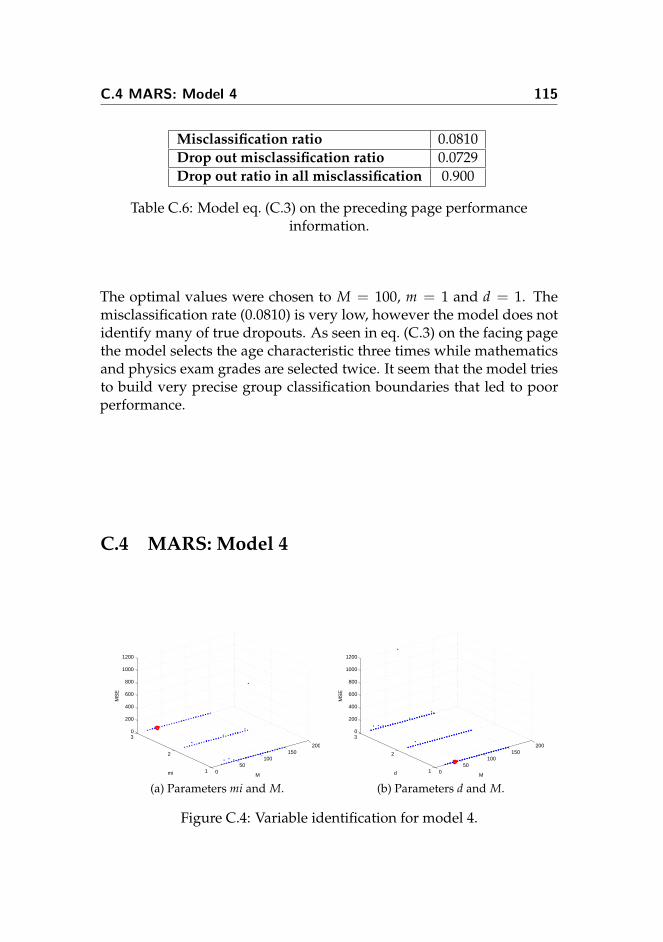
C.4 MARS: Model 4 115
Misclassification ratio 0.0810Drop out misclassification ratio 0.0729Drop out ratio in all misclassification 0.900
Table C.6: Model eq. (C.3) on the preceding page performanceinformation.
The optimal values were chosen to M = 100, m = 1 and d = 1. Themisclassification rate (0.0810) is very low, however the model does notidentify many of true dropouts. As seen in eq. (C.3) on the facing pagethe model selects the age characteristic three times while mathematicsand physics exam grades are selected twice. It seem that the model triesto build very precise group classification boundaries that led to poorperformance.
C.4 MARS: Model 4
050
100150
200
1
2
30
200
400
600
800
1000
1200
Mmi
MS
E
(a) Parameters mi and M.
050
100150
200
1
2
30
200
400
600
800
1000
1200
Md
MS
E
(b) Parameters d and M.
Figure C.4: Variable identification for model 4.

116 MARS Models for Every Semester
BF1 = max(0, ECTS R 1 + 0.72667)BF2 = max(0,−0.34271− chemistry exam grade)BF3 = max(0, physics exam grade + 0.64253)BF4 = max(0, shool GPA + 2.1348)BF5 = max(0, 1.61− Biotechnology programme)
y = 0.82796− 0.62631 · BF1 + 0.098617 · BF2 + 0.089562 · BF3 (C.4)− 0.060304 · BF4− 0.045833 · BF5
DD DP PP PDTrain 29 33 351 8Test 8 8 87 4
Table C.7: Predictions using model eq. (C.4)
Misclassification ratio 0.1004Drop out misclassification ratio 0.0777Drop out ratio in all misclassification 0.7736
Table C.8: Model eq. (C.4) performance information.
The optimal values are M = 50, mi = 1 and d = 1. In this case around50% dropouts were identified with 20-30% false alarm rate. All character-istics where chosen once and the model used 5 basic functions. Amongthe models for the second semester that use other techniques, the modelchose school exam grades and ratio of passed and taken ECST creditsafter the first semester.

C.5 MARS: Model 5 117
050
100150
200
1
2
30
1
2
3
4
5
6
7
x 105
Mmi
MS
E
(a) Parameters mi and M.
050
100150
200
1
2
30
1
2
3
4
5
6
7
x 105
Md
MS
E
(b) Parameters d and M.
Figure C.5: Variable identification for model 5.
C.5 MARS: Model 5
BF1 = max(0, mathematics exam grade + 0.11625)BF2 = max(0, physics level C + 0.051709)BF3 = max(0, ECTS R 1 + 1.6956)BF4 = max(0,−1.6956− ECTS R 1)BF5 = max(0,−2.6567− ECTS A 2)BF6 = max(0, 0.89165− ECTS T 2)BF7 = max(0, 0.97359− ECTS P 2)
y = 0.22933 + 0.042831 · BF1− 0.019974 · BF2− 0.11515 · BF3 (C.5)− 0.090297 · BF4 + 0.24416 · BF5− 0.39499 · BF6 + 0.38565 · BF7
DD DP PP PDTrain 9 6 359 0Test 3 1 91 0
Table C.9: Predictions using model eq. (C.5)
The optimal values were chosen to M = 30, mi = 1 and d = 1. Themodel performs with a false alarm rate at zero and identifies 63% of alldropouts after third semester.

118 MARS Models for Every Semester
Misclassification ratio 0.0149Drop out misclassification ratio 0.0149Drop out ratio in all misclassification 1
Table C.10: Model eq. (C.5) on the preceding page performanceinformation.
C.6 MARS: Model 6
050
100150
200
1
2
30
1
2
3
4
5
6
7
x 105
Mmi
MS
E
(a) Parameters mi and M.
050
100150
200
1
2
30
1
2
3
4
5
6
7
x 105
Md
MS
E
(b) Parameters d and M.
Figure C.6: Variable identification for model 6.

C.6 MARS: Model 6 119
BF1 = max(0,−1.4015− ECTS R 3)BF2 = max(0, ECTS R 2 + 1.2037)BF3 = max(0, mathematics exam grade− 1.8054)BF4 = max(0, ECTS P 3 + 1.8701)BF5 = max(0, mathematics level B + 0.089924)BF6 = max(0, ECTS R 2 + 1.0254)BF7 = max(0, physics levelB + 0.051778)BF8 = max(0, physics exam grade− 1.6228)BF9 = max(0,−0.97217− ECTS P 2)
BF10 = max(0,−1.0282− ECTS T 2)BF11 = max(0,−2.0505− school GPA)
BF12 = max(0,−1.9469− ECTS P 2)BF13 = max(0, ECTS P 3 + 1.2039)BF14 = max(0,−1.2039− ECTS T 3)BF15 = max(0, GPA O 2 + 1.8835)BF16 = max(0,−1.2209−GPA S 2)BF17 = max(0, GPA O 2 + 0.30493)BF18 = max(0,−0.30493−GPA O 2)BF19 = max(0, ECTS A 3 + 1.7934)BF20 = max(0, ECTS A 3 + 1.0439)BF21 = max(0,−1.0439− ECTS A 3)BF22 = max(0,−2.1681− ECTS A 3)
y = 1.6134 + 0.06998 · BF1− 1.1624 · BF2 + 0.55959 · BF3 (C.6)− 0.3315 · BF4 + 0.045761 · BF5 + 1.1938 · BF6− 0.02721 · BF7+ 0.24682 · BF8 + 1.0294 · BF9− 0.93138 · BF10− 0.15034 · BF11− 0.91951 · BF12 + 0.3205 · BF13− 0.20559 · BF14− 0.22006 · BF15+ 0.16247 · BF16 + 0.20949 · BF17− 0.23919 · BF18− 1.1545 · BF19+ 1.1628 · BF20− 0.80525 · BF21 + 0.76949 · BF22
The optimal values are M = 51, mi = 1 and d = 1. The model performsdecent as it identifies 58% of all dropouts with 2% misclassification rate.

120 MARS Models for Every Semester
DD DP PP PDTrain 9 5 358 1Test 1 2 89 2
Table C.11: Predictions using model eq. (C.6) on the preceding page
Misclassification ratio 0.0235Drop out misclassification ratio 0.0171Drop out ratio in all misclassification 0.7273
Table C.12: Model eq. (C.6) on the preceding page performanceinformation.
However the model complexity is just unacceptable. The model used 22basic functions.
C.7 MASR: Model 7
050
100150
200
1
2
30
2
4
6
8
10
12
x 106
Mmi
MS
E
(a) Parameters mi and M.
050
100150
200
1
2
30
2
4
6
8
10
12
x 106
Md
MS
E
(b) Parameters d and M.
Figure C.7: Variable identification for model 7.

C.7 MASR: Model 7 121
BF1 = max(0, physics exam grade + 1.9439)BF2 = max(0,−0.73559− ECTS R 4)BF3 = max(0, 0.48563− physics exam grade)BF4 = max(0, age + 0.91393)BF5 = max(0,−0.91393− age)BF6 = max(0,−1.0295− ECTS T 2)BF7 = max(0, ECTS P 2 + 1.0121)BF8 = max(0, age + 0.88543)BF9 = max(0, GPA S 2 + 1.7638)
BF10 = max(0, 1.5915−GPA S 2)BF11 = max(0, ECTS P 2 + 2.0065)BF12 = max(0, chemistry exam grade + 0.82668)BF13 = max(0, physics exam grade− 0.19409)BF14 = max(0, 0.19409− physics exam grade)BF15 = max(0, physics exam grade0− 0.68)BF16 = max(0, 0.68− physics exam grade)BF17 = max(0, school GPA + 0.11428)
y = 1.0553 + 0.3294 · BF1 + 0.030421 · BF2− 0.67208 · BF3 (C.7)− 3.3647 · BF4− 0.64363 · BF5− 0.53151 · BF6 + 0.46353 · BF7+ 3.3485 · BF8− 0.11542 · BF9− 0.10965 · BF10− 0.47915 · BF11+ 0.024294 · BF12− 1.9305 · BF13 + 2.194 · BF14 + 1.6114 · BF15− 1.2111 · BF16− 0.034379 · BF17
DD DP PP PDTrain 2 3 359 0Test 0 1 91 0
Table C.13: Predictions using model eq. (C.7)
The optimal values are M = 100, mi = 1 and d = 1. The model identit-ies passed students well, but it fails to identify dropouts. It is becausemodel was trained with merely 5 dropouts in the training data set. Equa-tion (C.7) is a complex model as it has 17 basic functions and some of

122 MARS Models for Every Semester
Misclassification ratio 0.0088Drop out misclassification ratio 0.0088Drop out ratio in all misclassification 1
Table C.14: Model eq. (C.7) on the preceding page performanceinformation.
the characteristics were chosen several times. For example, physic examgrade was chosen 4 times.
C.8 MARS: Model 8
050
100150
200
1
2
30
0.5
1
1.5
2
x 105
Mmi
MS
E
(a) Parameters mi and M.
050
100150
200
1
2
30
0.5
1
1.5
2
x 105
Md
MS
E
(b) Parameters d and M.
Figure C.8: Variable identification for model 8.
BF1 = max(0,−2.2372− ECTS A 3)BF2 = max(0,−2.003− ECTS R 5)BF3 = max(0,−1.99− ECTS R 3)BF4 = max(0,−2.7095− ECTS T 5)BF5 = max(0,−0.65111− ECTS T 1)
y = −0.0028257 + 0.18207 · BF1 + 0.11221 · BF2 (C.8)+ 0.074542 · BF3 + 1.0831 · BF4 + 0.095512 · BF5
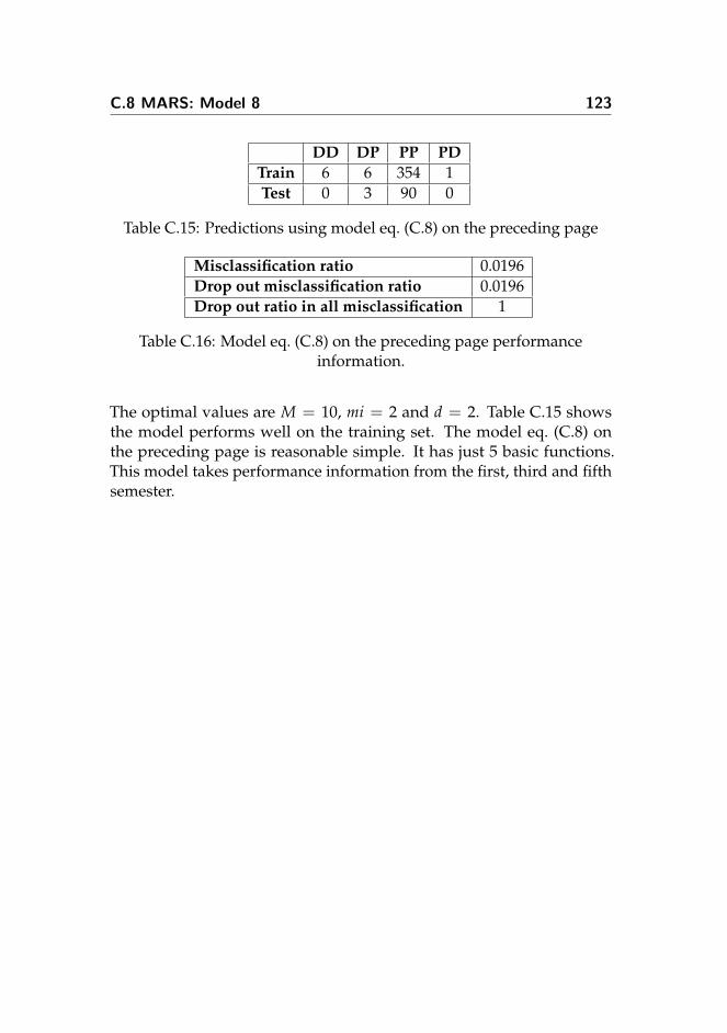
C.8 MARS: Model 8 123
DD DP PP PDTrain 6 6 354 1Test 0 3 90 0
Table C.15: Predictions using model eq. (C.8) on the preceding page
Misclassification ratio 0.0196Drop out misclassification ratio 0.0196Drop out ratio in all misclassification 1
Table C.16: Model eq. (C.8) on the preceding page performanceinformation.
The optimal values are M = 10, mi = 2 and d = 2. Table C.15 showsthe model performs well on the training set. The model eq. (C.8) onthe preceding page is reasonable simple. It has just 5 basic functions.This model takes performance information from the first, third and fifthsemester.

124 MARS Models for Every Semester

APPENDIX D
MATLAB Code
D.1 File: Main.m
1 % Read data frol .xlsx file2 [num1 bio,txt1 bio,raw1 bio] =...3 xlsread('early warning 2 tekbio.xlsx',2,'A2:V210');4 [num2 bio,txt2 bio,raw2 bio] =...5 xlsread('early warning 2 tekbio.xlsx',1,'A2:J3021');6 [num1 dis,txt1 dis,raw1 dis] =...7 xlsread('early warning 2 design.xlsx',2,'A2:V613');8 [num2 dis,txt2 dis,raw2 dis] =...9 xlsread('early warning 2 design.xlsx',1,'A2:J9360');
10 [num1 mat,txt1 mat,raw1 mat] =...11 xlsread('early warning system 2 mat.xlsx',2,'A2:V406');12 [num2 mat,txt2 mat,raw2 mat] =...13 xlsread('early warning system 2 mat.xlsx',1,'A2:J5956');14 [num1 btek,txt1 btek,raw1 btek] =...15 xlsread('early warning 2 biotek.xlsx',1,'A2:V522');16 [num2 btek,txt2 btek,raw2 btek] =...17 xlsread('early warning 2 biotek.xlsx',2,'A2:J7323');18 %% Data of BC Biotechnology programme19 prog = 1;

126 MATLAB Code
20 num2 bio = SortExamps(raw2 bio,num2 bio,num1 bio,0);21 [stat num bio BC,stat txt bio BC] = Status(raw1 bio,...22 num1 bio,num2 bio,prog);23 num2 bio BC = PerformanceInformation(num2 bio,...24 stat num bio BC, prog);25 info bio BC = PersonalInfo(raw1 bio,num1 bio,...26 stat num bio BC);27 info s bio BC = PersonalInfo short(raw1 bio,num1 bio,...28 stat num bio BC);29 [ECTS T bio BC, ECTS P bio BC, ECTS R bio BC,...30 ECTS A bio BC,ECTS L bio BC, GPA S bio BC,...31 GPA O bio BC] = PerformanceInfo Summury...32 (stat num bio BC, num2 bio BC,prog);33 % Data of BC Design and Inovation programme34 prog = 1;35 num2 dis = SortExamps(raw2 dis,num2 dis,num1 dis,0);36 [stat num dis BC,stat txt dis BC] = Status(raw1 dis,...37 num1 dis,num2 dis,prog);38 num2 dis BC = PerformanceInformation(num2 dis,...39 stat num dis BC, prog);40 info dis BC = PersonalInfo(raw1 dis,num1 dis,stat num dis BC);41 info s dis BC = PersonalInfo short(raw1 dis,...42 num1 dis,stat num dis BC);43 [ECTS T dis BC, ECTS P dis BC, ECTS R dis BC,...44 ECTS A dis BC, ECTS L dis BC,GPA S dis BC,...45 GPA O dis BC]= PerformanceInfo Summury...46 (stat num dis BC, num2 dis BC,prog);47 % Data of BC Mathematics and Technologu programme48 prog = 1;49 num2 mat = SortExamps(raw2 mat,num2 mat,num1 mat,0);50 [stat num mat BC,stat txt mat BC] =...51 Status(raw1 mat,num1 mat,num2 mat,prog);52 num2 mat BC = PerformanceInformation...53 (num2 mat, stat num mat BC, prog);54 info mat BC = PersonalInfo(raw1 mat,num1 mat,stat num mat BC);55 info s mat BC = PersonalInfo short...56 (raw1 mat,num1 mat,stat num mat BC);57 [ECTS T mat BC, ECTS P mat BC, ECTS R mat BC,...58 ECTS A mat BC, ECTS L mat BC, GPA S mat BC,...59 GPA O mat BC] = PerformanceInfo Summury...60 (stat num mat BC, num2 mat BC,prog);61 % Data of BC Biomedicine programme62 prog = 1;63 num2 btek = SortExamps(raw2 btek,num2 btek,num1 btek, 1);64 [stat num btek BC,stat txt btek BC] =...65 Status(raw1 btek,num1 btek,num2 btek,prog);66 num2 btek BC = PerformanceInformation...

D.1 File: Main.m 127
67 (num2 btek, stat num btek BC, prog);68 info btek BC = PersonalInfo...69 (raw1 btek,num1 btek,stat num btek BC);70 info s btek BC = PersonalInfo short...71 (raw1 btek,num1 btek,stat num btek BC);72 [ECTS T btek BC, ECTS P btek BC, ECTS R btek BC,...73 ECTS A btek BC,ECTS L btek BC, GPA S btek BC,...74 GPA O btek BC] = PerformanceInfo Summury...75 (stat num btek BC, num2 btek BC,prog);76 % BC data concatenation77 stat num BC= [stat num bio BC;stat num dis BC;...78 stat num mat BC; stat num btek BC];79 stat txt BC =[stat txt bio BC;stat txt dis BC;...80 stat txt mat BC;stat txt btek BC];81 ECTS T BC = [ECTS T bio BC; ECTS T dis BC;...82 ECTS T mat BC; ECTS T btek BC;];83 ECTS P BC = [ECTS P bio BC; ECTS P dis BC;...84 ECTS P mat BC;ECTS P btek BC];85 ECTS A BC = [ECTS A bio BC; ECTS A dis BC;...86 ECTS A mat BC;ECTS A btek BC;];87 ECTS L BC = [ECTS L bio BC; ECTS L dis BC;...88 ECTS L mat BC;ECTS L btek BC];89 ECTS R BC = [ECTS R bio BC; ECTS R dis BC;...90 ECTS R mat BC;ECTS R btek BC];91 GPA S BC = [GPA S bio BC; GPA S dis BC;...92 GPA S mat BC;GPA S btek BC];93 GPA O BC = [GPA O bio BC; GPA O dis BC;...94 GPA O mat BC;GPA O btek BC];95 info BC=[info bio BC;info dis BC;...96 info mat BC;info btek BC];97 info s BC=[info s bio BC;info s dis BC;...98 info s mat BC;info s btek BC];99 %%
100 % Divides BC in to maint training and test sets (9:1)101 % Randomize index for data division102 index = randperm(size(info BC,1));103 % Counts 10proc. for test set.104 BC text num = round(size(index,2)*0.0);105 %Divides to general training and test set106 % Test set107 stat num BC test= stat num BC(index(1:BC text num),:);108 stat txt BC test =stat txt BC(index(1:BC text num),:);109 ECTS T BC test = ECTS T BC(index(1:BC text num),:);110 ECTS P BC test = ECTS P BC(index(1:BC text num),:);111 ECTS A BC test = ECTS A BC(index(1:BC text num),:);112 ECTS L BC test = ECTS L BC(index(1:BC text num),:);113 ECTS R BC test = ECTS R BC(index(1:BC text num),:);

128 MATLAB Code
114 GPA S BC test = GPA S BC(index(1:BC text num),:);115 GPA O BC test = GPA O BC(index(1:BC text num),:);116 info BC test = info BC(index(1:BC text num),:);117 info s BC test = info s BC(index(1:BC text num),:);118 % Train set119 stat num BC train= stat num BC(index(BC text num+1: end),:);120 stat txt BC train =stat txt BC(index(BC text num+1: end),:);121 ECTS T BC train = ECTS T BC(index(BC text num+1: end),:);122 ECTS P BC train = ECTS P BC(index(BC text num+1: end),:);123 ECTS A BC train = ECTS A BC(index(BC text num+1: end),:);124 ECTS L BC train = ECTS L BC(index(BC text num+1: end),:);
D.2 File: Main LR.m
1 %%%%%%%%%%%%%%%%%%%%%%%%%%%%%%%%%%%%%%%%%%%%%%%%%%%%%%%%%%%2 % LR individual semester model training and testing3 % Final CART model determination and testing.4 %%%%%%%%%%%%%%%%%%%%%%%%%%%%%%%%%%%%%%%%%%%%%%%%%%%%%%%%%%%5 semester2 =0; semester =20;6 % Separates data set in to training and testing sets7 [train BC,records1, test BC, records2, name] =...8 DataDivision(semester,semester2, sem BC,...9 stat txt BC train, GPA O BC train, GPA S BC train,...
10 ECTS A BC train,ECTS P BC train,...11 ECTS T BC train,ECTS R BC train, ECTS L BC train,...12 info BC train);13 % Recoding students status in to numerical values14 % 1− drop out; 0 − pass15 train coding = zeros(size(train BC));16 train coding(strcmp(train BC,'drop out')) = 1;17 test coding = zeros(size(test BC));18 test coding(strcmp(test BC,'drop out')) = 1;19 % Seperates data set in to 10 folds20 Indices = crossvalind('Kfold', size(train BC,1), 10);21 B = [];22 % Estimates B for every fold23 for i = 1:1024 cros train = train coding((Indices 6=i));25 cros rec = records1((Indices 6=i),:);26 B(:,i) = glmfit(cros rec,...27 [cros train ones(size(cros train,1),1)],...28 'binomial', 'link', 'logit');29 end30 % Mean B

D.3 File: Main PCA.m 129
31 B Mean = (round(mean(B,2)*1000))/1000;32 [misclas(1,3), misclas(1,4) , misclas(1,2) , misclas(1,1),...33 notclass1] =Prediction num(1,B Mean, records1,...34 train coding);35 [misclas(2,3), misclas(2,4) , misclas(2,2) , misclas(2,1),...36 notclass2]=Prediction num(1,B Mean, records2,...37 test coding);38 Table(misclas);39 %% Final model determination40 S = [0 1 1 2 3 4 5 6; 20 0 1 2 3 4 5 6];41 Model = [1 2 3 4 5 6 7 8];42 file = 'Models new/lr %i.mat';43 type = 3;44 predict = FinalPrediction(S, Model, file, type,...45 info BC train, GPA O BC train, GPA S BC train,...46 ECTS P BC train, ECTS T BC train,...47 ECTS A BC train,ECTS R BC train,ECTS L BC train);48 Model = {'1';'2';'3';'4';'5';'6';'7';'8'};49 [drop,false,sem advance]=FinalEval(S(1,:),...50 stat num BC train, predict, sem BC,Model)51 %% Final model testing52 S = [0 2 3; 20 2 3];53 Model = [1 4 5];54 file = 'Models new/lr %i.mat';55 type = 3;
D.3 File: Main PCA.m
1 %%%%%%%%%%%%%%%%%%%%%%%%%%%%%%%%%%%%%%%%%%%%%%%%%%%%%%%%%%%2 % PCA−LR individual semester model training and testing.3 % Final PCA−LR model determination and testing.4 %%%%%%%%%%%%%%%%%%%%%%%%%%%%%%%%%%%%%%%%%%%%%%%%%%%%%%%%%%%5 semester2 =0; semester = 20;6 [train BC,records1, test BC, records2, name] =...7 DataDivision(semester,semester2, sem BC,...8 stat txt BC train, GPA O BC train, GPA S BC train,...9 ECTS A BC train,ECTS P BC train, ECTS T BC train,...
10 ECTS R BC train, ECTS L BC train,info s BC train);11 % Remove student with missing data and get status12 % numerical values13 index=any(isnan(records1),2) ;14 records1(index == 1,:) = [];15 train coding = double(strcmp(train BC, 'drop out'));16 test coding = double(strcmp(test BC, 'drop out'));

130 MATLAB Code
17 train coding(index == 1,:) = [];18 % Standatize data19 AMean = mean(records1);20 AStd = std(records1);21 [n,m] = size(records1);22 records1 = (records1 − repmat(AMean,[n 1]))...23 ./ repmat(AStd,[n 1]);24 % Performs cros validation for PCA25 k fold = crossvalind('Kfold', size(train coding,1), 10);26 PCALoadings = cell(1,10);27 PCAScores = cell(1,10);28 PCAVar = cell(1,10);29 % Ploting variance30 figure(); hold on;31 for i = 1:1032 [PCALoadings{i},PCAScores{i},PCAVar{i}]=...33 princomp(records1(k fold 6= i,:));34 plot(PCAVar{i}, '−o');35 end36 xlabel('PC'); ylabel('Explained variance'); hold off;37 figure(); hold on;38 for i = 1:1039 plot(100*cumsum(PCAVar{i})/sum(PCAVar{i}), '−o');40 end41 xlabel('PC'); ylabel('Accumulated explained variance');42 hold off;43 % Number of PCA for model44 number PCA = 8;45 % PCA for modeling46 [PCALoadings,PCAScores,PCAVar] = princomp(records1);47 Indices = crossvalind('Kfold', size(train coding,1), 10);48 B = zeros(number PCA,10);49 % Estimates B for every fold50 for i = 1:1051 cros train = train coding(Indices 6=i);52 cros rec = PCAScores((Indices 6=i),1:number PCA);53 B(:,i) = glmfit(cros rec,...54 [cros train ones(size(cros train,1),1)],...55 'binomial', 'link', 'logit','constant','off');56 end57 % Average of betas58 avrB=mean(B,2);59 % Prediction60 [misclas(1,3), misclas(1,4) , misclas(1,2) , misclas(1,1),...61 notclass1] =Prediction logistic(3, avrB,PCAScores...62 (:,1:number PCA), train coding);63 Table(misclas)

D.4 File: Main CART.m 131
D.4 File: Main CART.m
1 %%%%%%%%%%%%%%%%%%%%%%%%%%%%%%%%%%%%%%%%%%%%%%%%%%%%%%%%%%%2 % CART individual semester model training and testing.3 % Final CART model determination and testing.4 %%%%%%%%%%%%%%%%%%%%%%%%%%%%%%%%%%%%%%%%%%%%%%%%%%%%%%%%%%%5 % Individual semester model training6 semester2 =0; semester = 20;7 %Divides data in to training and testing set that8 % approximately where would be the same data structure9 [train BC,records1, test BC, records2, name] =...
10 DataDivision(semester, semester2, sem BC,...11 stat txt BC train, GPA O BC train, GPA S BC train,...12 ECTS A BC train,ECTS P BC train, ECTS T BC train,...13 ECTS R BC train, ECTS L BC train,info s BC train);14 % Build the CART tree15 t=classregtree(records1,train BC, 'name', name,...16 'method', 'classification','minparent', 2,...17 'splitcriterion','twoing');18 view(t);19 % Search for the best pruning level20 [b,l] = Cost Plot(t, records1, train BC)21 % Prunes the tree22 t prune= prune(t, 'level',l);23 view(t prune);24 % Model performance table25 [misclas(1,3), misclas(1,4) , misclas(1,2) , misclas(1,1)]...26 = Prediction txt(1,t prune, records1, train BC);27 [misclas(2,3), misclas(2,4) , misclas(2,2) , misclas(2,1)]...28 = Prediction txt(1,t prune, records2, test BC);29 Table(misclas);30 %% Final model determination31 S = [0 2 3 4 6; 20 2 3 4 6];32 Model = [1 4 5 6 8];33 file = 'Models new/cart %i.mat';34 type = 1;35 predict = FinalPrediction(S, Model, file, type,...36 info s BC train, GPA O BC train, GPA S BC train,...37 ECTS P BC train, ECTS T BC train,...38 ECTS A BC train,ECTS R BC train,ECTS L BC train);39 Model = {'1';'4';'5';'6';'8'};40 [drop,false,sem advance]=FinalEval(S(1,:),...41 stat num BC train, predic, sem BC,Model)42 %% Final model43 S = [0 2 3; 20 2 3];

132 MATLAB Code
44 Model = [1 4 5];45 file = 'Models new/cart %i.mat';46 type = 1;47 predict = FinalPrediction(S, Model, file, type,...48 info s BC test, GPA O BC test, GPA S BC test,....49 ECTS P BC test, ECTS T BC test,...
D.5 File: Main Bagging.m
1 %%%%%%%%%%%%%%%%%%%%%%%%%%%%%%%%%%%%%%%%%%%%%%%%%%%%%%%%%%%2 % CART Bagging individual semester model training and3 % testing. Final CART bagging model determination4 % and testing.5 %%%%%%%%%%%%%%%%%%%%%%%%%%%%%%%%%%%%%%%%%%%%%%%%%%%%%%%%%%%6 semester2 = 20; semester = 0;7 % Separates data set in to training and testing sets8 [train BC,records1, test BC, records2, name,stud id]...9 = DataDivision(semester,semester2, sem BC,...
10 stat txt BC train, GPA O BC train,GPA S BC train,...11 ECTS A BC train,ECTS P BC train,ECTS T BC train,...12 ECTS R BC train, ECTS L BC train,info BC train);13 err = zeros(500,5);14 % Model building15 for i = 1 :516 fprintf('Step %f', i);17 B = TreeBagger(500,records1,train BC,'OOBPred',...18 'on','Method','classification','OOBVarImp', 'on');19 err(:,i) = oobError(B);20 end21 figure('Name', 'Mean'); plot(mean(err,2));22 xlabel('Number of grown trees')23 ylabel('Mena of out−of−bag classification error')24 figure('Name','STD'); plot(std(err,0,2));25 xlabel('Number of grown trees')26 ylabel...27 ('Standart deviation of out−of−bag classification error')28 % Define minimal number of trees for the semester model29 min tree = 300;30 B1 = TreeBagger(min tree,records1,train BC,'OOBPred',...31 'on','Method','classification');32 [misclas(1,3), misclas(1,4) , misclas(1,2) , misclas(1,1)]...33 = Prediction(2,B1, records1, train BC);34 [misclas(2,3), misclas(2,4) , misclas(2,2) , misclas(2,1)]...35 = Prediction(2,B1, records2, test BC)

D.6 File: Main RF.m 133
36 Table(misclas);37 %% Final model determination38 S = [0 1 1 2 3 4 5 6; 20 0 1 2 3 4 5 6];39 Model = [1 2 3 4 5 6 7 8];40 file = 'Models new/bagging %i.mat';41 type = 2;42 predict = FinalPrediction(S, Model, file, type,...43 info BC train, GPA O BC train, GPA S BC train,...44 ECTS P BC train, ECTS T BC train, ECTS A BC train,...45 ECTS R BC train,ECTS L BC train);46 Model = {'1';'2';'3';'4';'5';'6';'7';'8'};47 [drop,false,sem advance]=FinalEval(S(1,:),...48 stat num BC train, predict,sem BC,Model)49 %% Final model testing50 S = [0 2; 20 2];51 Model = [1 4];52 file = 'Models new/bagging %i.mat';53 type = 2;54 predict = FinalPrediction(S, Model, file, type,...55 info BC test, GPA O BC test, GPA S BC test,...56 ECTS P BC test, ECTS T BC test, ECTS A BC test,...57 ECTS R BC test,ECTS L BC test);58 Model = {'1';'4'};59 [drop,false,sem advance]=FinalEval(S(1,:),...60 stat num BC test, predict,sem BC test,Model)
D.6 File: Main RF.m
1 %%%%%%%%%%%%%%%%%%%%%%%%%%%%%%%%%%%%%%%%%%%%%%%%%%%%%%%%%%%2 % Random forest individual semester model training and3 % testing. Final RF model determination and testing.4 %%%%%%%%%%%%%%%%%%%%%%%%%%%%%%%%%%%%%%%%%%%%%%%%%%%%%%%%%%%5 semester2 =1; semester =0;6 % Separates data set in to training and testing sets7 [train BC,records1, test BC, records2, name] = ....8 DataDivision(semester, semester2, sem BC,...9 stat txt BC train, GPA O BC train, GPA S BC train,...
10 ECTS A BC train,ECTS P BC train, ECTS T BC train,....11 ECTS R BC train, ECTS L BC train,info BC train);12 train coding = ones(size(train BC));13 train coding(strcmp(train BC,'drop out')) = −1;14 train = ones(size(train BC));15 train(strcmp(train BC,'drop out')) = −1;16 test coding = ones(size(test BC));

134 MATLAB Code
17 test coding(strcmp(test BC,'drop out')) = 1;18 % Removes students with missig values19 records= records1;20 index=any(isnan(records),2) ;21 records(index == 1,:) = [];22 train coding(index == 1,:) = [];23 % Setting extra optioons for modeling24 clear extra options25 extra options.importance = 1;26 extra options.proximity = 1;27 %% Most important variables detection, using average28 % of 10 models29 test = 10;30 mean decrease = zeros(size(records,2),test);31 gini decrease = zeros(size(records,2),test);32 for i = 1:test33 model = classRF train(records,...34 train coding,0,0,extra options);35 mean decrease(:,i) = model.importance(:,end−1);36 gini decrease(:,i) = model.importance(:,end);37 end38 mean decrease avr = mean(mean decrease,2);39 gini decrease avr = mean(mean decrease,2);40 figure('Name','Mean decrease in Accuracy');41 bar(model.importance(:,end−1));42 xlabel('feature');ylabel('magnitude');43 figure('Name','Mean decrease in Gini index');44 bar(model.importance(:,end));45 xlabel('feature');ylabel('magnitude');46 %% Searching for the good MTRY using 5 fold cross validation47 % Determining important variables48 important varb = [1 4 5 8 9 14 18 19 20 21 23];49 records red1 = records(:,important varb);50 records red2 = records2(:,important varb);51 % Determining parameters for the test52 kfold = 5 ;53 Indices = crossvalind('Kfold', size(train coding,1), kfold);54 MTRY = size(records red1,2);55 dd = zeros(kfold,1); pd = zeros(kfold,1); dp = zeros(kfold,1);56 pp = zeros(kfold,1); dd avr = zeros(MTRY,1);57 pd avr = zeros(MTRY,1); dd std = zeros(MTRY,1);58 pd std = zeros(MTRY,1);59 for i = 1:MTRY60 for k = 1:kfold61 model = classRF train(records red1...62 (Indices 6=k,:), train coding(Indices...63 6=k,:),500,i,extra options);

D.6 File: Main RF.m 135
64 [pp, pd(k,1), dp, dd(k,1)] = Prediction RF...65 (model, records red1(Indices ==k,:),....66 train coding(Indices == k,:));67 end68 dd avr(floor(i/5)+1,1) = mean(dd);69 pd avr(floor(i/5)+1,1) = mean(pd);70 dd std(floor(i/5)+1,1) = std(dd);71 pd std(floor(i/5)+1,1) = std(pd);72 end73 figure('Name','Mean'); plot(1:MTRY,dd avr, '−b');74 hold on; plot(1:MTRY,pd avr,'−r'); hold off;75 xlabel('MTRY'); ylabel('Mean of classifications');76 legend('DD', 'PD')77 figure('Name', 'STD'); plot(1:MTRY,dd std, '−b');78 hold on; plot(1:MTRY,pd std,'−r'); hold off;79 xlabel('MTRY'); ylabel('Standard deviation Classifications');80 legend('DD', 'PD')81 %% Searching for the good NTREE using 5 fold cross validation82 MTRY = 4;83 dd = zeros(kfold,1); pd = zeros(kfold,1); dp = zeros(kfold,1);84 pp = zeros(kfold,1); dd avr = zeros(50,1);85 pd avr = zeros(50,1); dd std = zeros(50,1);86 pd std = zeros(50,1);87 NTREE = 500;88 for i = 1:10:NTREE89 for k = 1:kfold90 model = classRF train(records red1(Indices...91 6=k,:),train coding(Indices 6=k,:)....92 ,i,MTRY,extra options);93 [pp, pd(k,1), dp, dd(k,1)] = Prediction RF...94 (model, records red1(Indices ==k,:),...95 train coding(Indices == k,:));96 end97 dd avr(floor(i/10)+1,1) = mean(dd);98 pd avr(floor(i/10)+1,1) = mean(pd);99 dd std(floor(i/10)+1,1) = std(dd);
100 pd std(floor(i/10)+1,1) = std(pd);101 end102 figure('Name','Mean'); plot(1:50,dd avr, '−b');103 hold on; plot(1:50,pd avr,'−r'); hold off;104 xlabel('NTREE'); ylabel('Mean of classifications');105 legend('DD', 'PD')106 set(gca,'XTickLabel',0:50:500,'XTick',0:5:50);107 figure('Name', 'STD'); plot(1:50,dd std, '−b');108 hold on; plot(1:50,pd std,'−r'); hold off;109 xlabel('NTREE');110 ylabel('Standard deviation Classifications');

136 MATLAB Code
111 legend('DD', 'PD');112 set(gca,'XTickLabel',0:50:500,'XTick',0:5:100);113 %% Building final semester model114 NTREE = 200;115 model = classRF train(records red1,...116 train coding,NTREE,MTRY,extra options);117 [misclas(1,3), misclas(1,4) , misclas(1,2) , misclas(1,1)]...118 = Prediction RF(model, records red1, train coding);119 [misclas(2,3), misclas(2,4) , misclas(2,2) , misclas(2,1)]...120 = Prediction RF(model, records red2, test coding);121 Table(misclas);122 %% Determing final model123 S = [0 1 1 2 3 4 5 6; 20 0 1 2 3 4 5 6 ];124 Model = [1 2 3 4 5 6 7 8];125 file = 'Models new/RF %i .mat';126 type = 5;127 predict = FinalPrediction(S, Model, file, type,...128 info BC train, GPA O BC train, GPA S BC train,...129 ECTS P BC train, ECTS T BC train,...130 ECTS A BC train,ECTS R BC train,ECTS L BC train);131 predict(predict == 1) = 0; predict(predict == −1) = 1;132 Model = {'1';'2';'3';'4';'5';'6';'7';'8'};133 [drop,false,sem advance]=FinalEval(S(1,:),...134 stat num BC train, predict, sem BC,Model)135 %% Final model testing136 S = [0 2; 20 2];137 Model = [1 4];138 file = 'Models new/RF %i .mat';139 type = 5;140 predict = FinalPrediction(S, Model, file, type,...141 info BC test, GPA O BC test, GPA S BC test,...142 ECTS P BC test, ECTS T BC test, ECTS A BC test,...143 ECTS R BC test,ECTS L BC test);144 predict(predict == 1) = 0; predict(predict == −1) = 1;145 Model = {'1';'4'};146 [drop,false,sem advance]=FinalEval(S(1,:),...147 stat num BC test, predict, sem BC test,Model)
D.7 File: Main MARS.m
1 %%%%%%%%%%%%%%%%%%%%%%%%%%%%%%%%%%%%%%%%%%%%%%%%%%%%%%%%%%%2 % MARS individual semester model training and testing.3 % Final MARS model determination and testing.4 %%%%%%%%%%%%%%%%%%%%%%%%%%%%%%%%%%%%%%%%%%%%%%%%%%%%%%%%%%%

D.7 File: Main MARS.m 137
5 % Searching for best M, mi and d variables combination...6 % that would give the smalest MSE7 % Variable semeter8 A = [0 1 1 2 3 4 5 6; 20 0 1 2 3 4 5 6];9 % Grid for M, mi and d
10 M vec = 21:5:151; mi vec = 1:3; d vec = 1:3;11 N = length(M vec) * 3 * 3;12 [MIM,DM,MM] = meshgrid(mi vec,d vec,M vec);13 MARSpar = [MM(:),MIM(:),DM(:)];14 % Get some MATLAB workers15 matlabpool open SGE 15;16 k = 1;17 % Result matrix18 res = zeros(N*8,9);19 fprintf(1, 'Beginning MARS calculations\n\n');20 % Standardization values matrix21 mean est = cell(1,8); std est = cell(1,8);22 starttime=tic;23 try24 for i = 1:825 semester2 = A(1,i); semester = A(2,i);26 % Separates data set in to training and testing sets27 [train BC,records1, dummy1, dummy2, dummy3] =...28 DataDivision( semester, semester2, sem BC,...29 stat txt BC train, GPA O BC train,...30 GPA S BC train, ECTS A BC train,...31 ECTS P BC train, ECTS T BC train,...32 ECTS R BC train, ECTS L BC train,info BC train);33 mean est{i} = nanmean(records1);34 std est{i} = nanstd(records1);35 cent = bsxfun(@minus,records1, mean est{i});36 records1 = bsxfun(@rdivide,cent,std est{i});37 train coding=strcmp(train BC,'drop out');38 parfor k = (1+(i−1)*N):(N+(i−1)*N)39 tmpi = k − (i−1)*N;40 % This is a var running between 1 and N41 M = MM(tmpi);42 mi = MIM(tmpi);43 d = DM(tmpi);44 fprintf(1,'i=%i\tk=%i\tM=%i\tmi=%i\td=%i\n',...45 i, k, M, mi, d);46 params = aresparams(M, 5, false, [], mi, d);47 [taMSE,taRMSE,taRRMS,taR2] =...48 arescv(records1, train coding,...49 params, [], 5,[],[],[],0);50 res(k,:) = [i k M mi d taMSE taRMSE taRRMS taR2];51 end

138 MATLAB Code
52 end53 catch err54 disp(err);55 end56 toc(starttime);57 save(sprintf('mars res %s.mat',datestr(now(),...58 'yyyymmddHHMM')), mean est,std est,res);59 matlabpool close;60 %% Individual semester model building61 semester2 =0; semester = 20;62 % Separates data set in to training and testing sets63 [train BC,records1, test BC, records2, name] =...64 DataDivision(semester, semester2, sem BC,...65 stat txt BC train, GPA O BC train, GPA S BC train,...66 ECTS A BC train,ECTS P BC train, ECTS T BC train,...67 ECTS R BC train, ECTS L BC train,info BC train);68 % Standardization69 mean estm = nanmean(records1);70 std estm = nanstd(records1);71 Cent = bsxfun(@minus,records1,mean estm);72 records1 = bsxfun(@rdivide,Cent,std estm);73 Cent = bsxfun(@minus,records2,mean estm);74 records2 = bsxfun(@rdivide,Cent,std estm);75 train coding = zeros(size(train BC));76 train coding(strcmp(train BC,'drop out')) = 1;77 test coding = zeros(size(test BC));78 test coding(strcmp(test BC,'drop out')) = 1;79 % Setting parameters80 M = 10; mi = 1; d = 1;81 params = aresparams(M, 5, false, [], mi, d);82 % Model building83 model = aresbuild(records1, train coding, params)84 ModelF = struct('model', model,...85 'mean estm',mean estm,'std estm',std estm);86 % Model output in mathematical form87 B = areseq(model, 5)88 [misclas(1,3), misclas(1,4) , misclas(1,2) , misclas(1,1)]...89 = Prediction num(2,model, records1, train coding);90 [misclas(2,3), misclas(2,4) , misclas(2,2) , misclas(2,1)]...91 = Prediction num(2,model, records2, test coding);92 Table(misclas);93 %% Final model determination94 S = [0 1 1 2 3 4 5 6; 20 0 1 2 3 4 5 6];95 Model = [1 2 3 4 5 6 7 8];96 file = 'Models new/mars %i.mat';97 type = 4;98 predict = FinalPrediction(S, Model, file, type,...

D.8 Function: Round ECTS.m 139
99 info BC train, GPA O BC train, GPA S BC train,...100 ECTS P BC train, ECTS T BC train,ECTS A BC train,...101 ECTS R BC train,ECTS L BC train);102 Model = {'1';'2';'3';'4';'5';'6';'7';'8'};103 [drop,false,sem advance]=FinalEval(S(1,:),...104 stat num BC train, predict, sem BC,Model)105 %% Final model testing106 S = [0 2; 20 2];107 Model = [1 4];108 file = 'Models new/mars %i.mat';109 type = 4;110 predict = FinalPrediction(S, Model, file, type,...111 info BC test, GPA O BC test, GPA S BC test,...112 ECTS P BC test, ECTS T BC test, ECTS A BC test,...113 ECTS R BC test,ECTS L BC test);114 Model = {'1';'4'};115 [drop,false,sem advance]=FinalEval(S(1,:),....116 stat num BC test, predict,sem BC test,Model)
D.8 Function: Round ECTS.m
1 %%%%%%%%%%%%%%%%%%%%%%%%%%%%%%%%%%%%%%%%%%%%%%%%%%%%%%%%%%%2 % Raunding ECTS credits measurments that value of module3 % after division of five would be 0.4 % Adress: Main5 %%%%%%%%%%%%%%%%%%%%%%%%%%%%%%%%%%%%%%%%%%%%%%%%%%%%%%%%%%%6 function [rounded] = Round ECTS(A)7 for i = 1:size(A,1)8 for j = 2:size(A,2)9 if mod(A(i,j),1) < 2.5
10 rounded(i,j) = A(i,j) − mod(A(i,j),5);11 else12 rounded(i,j) = A(i,j) + 5 − mod(A(i,j),5);13 end14 end15 end16 rounded(:,1) = A(:,1);
D.9 Function: SortExamps.m
1 %%%%%%%%%%%%%%%%%%%%%%%%%%%%%%%%%%%%%%%%%%%%%%%%%%%%%%%%%%%

140 MATLAB Code
2 % Updates num [program] matrix. Output: 1 col: student ID, 23 % col: number of semester, 3 col: program level,4 % 4 col: mark, 5 col: ECTS.5 % Adress: Main6 %%%%%%%%%%%%%%%%%%%%%%%%%%%%%%%%%%%%%%%%%%%%%%%%%%%%%%%%%%%7 function [num] = SortExamps(raw2,num2,num1, type)8 [num code,txt code,raw code] =...9 xlsread('semester coding.xlsx',1,'A1:B30');
10 num(:,1) = num2(:,1);11 % Converting semester name in to digits12 % Coding is in excel file: semester coding.xlsx13 for i = 1:size(raw code,1)14 [r,c] = find(strcmp(raw2,txt code(i)));15 if ¬isempty(r)16 num(r,2) = num code(i,1);17 r = [];18 end19 end20 % Chnging Marks from string to numbers21 % −20 − not attendet exam; 20 − passed exam;22 % 1 − BC program;2 − MC program23 for i = 1:size(raw2,1)24 if strcmp(raw2(i,2), 'CBAC04')25 num(i,3) = 1;26 elseif strcmp(raw2(i,2), 'CKAN06DK') | | ...27 strcmp(raw2(i,2), 'CKAN10DK')28 num(i,3) = 2;29 end30 if strcmp(raw2(i,2), 'CBAC04') | | ...31 strcmp(raw2(i,2), 'CKAN06DK')...32 | | strcmp(raw2(i,2), 'CKAN10DK')33 if strcmp(raw2(i,6),'EM')34 num(i,4) = −20;35 elseif strcmp(raw2(i,6),'BE')36 num(i,4) = 20;37 else38 num(i,4) = str2double(raw2(i,6));39 end40 if type ==141 num(i,5) = num2(i,8);42 else43 num(i,5) = str2double(raw2(i,8));44 end45 end46 end47 % Sorting data according semesters48 for i=1:size(num1,1)

D.10 Function: Status.m 141
49 begin = find(num ==num1(i,1),1);50 all = size(find(num ==num1(i,1)),1);51 extract = num(begin:all+begin−1,:);52 num(begin:begin+all−1,:) = sortrows(extract,[3 2]);53 extract=[];54 end
D.10 Function: Status.m
1 %%%%%%%%%%%%%%%%%%%%%%%%%%%%%%%%%%%%%%%%%%%%%%%%%%%%%%%%%%%2 % Extracts student status. In stat num first col coded3 % status (1 − drop out, 0 − pass) and second student ID4 % In stat txt status in text5 % Adress: Main6 %%%%%%%%%%%%%%%%%%%%%%%%%%%%%%%%%%%%%%%%%%%%%%%%%%%%%%%%%%%7 function [stat num, stat txt] = Status(raw1,num1,num2, prog)8 % prog ==1 corresponds to BSc9 if prog == 1
10 txt1 = 'CBAC04';11 txt2 = 'CBAC04';12 else13 txt1 = 'CKAN06DK';14 txt2 = 'CKAN10DK';15 end16 stat num = []; stat txt = {};17 for i = 1:size(raw1,1)18 if strcmp(raw1(i,19),txt1) | | strcmp(raw1(i,19),txt2)19 if strcmp(raw1(i,20),'afbrudt')20 stat num( end+1,1) = 1;21 stat num( end,2) = num1(i,1);22 stat txt( end+1,1) = {'drop out'};23 elseif strcmp(raw1(i,20),'afsluttet')24 stat num( end+1,1) = 0;25 stat num( end,2) = num1(i,1);26 stat txt( end+1,1) = {'pass'};27 end28 end29 end
D.11 Function: PersonalInfo short.m

142 MATLAB Code
1 %%%%%%%%%%%%%%%%%%%%%%%%%%%%%%%%%%%%%%%%%%%%%%%%%%%%%%%%%%%2 % Makes personal information matrix with out dummy3 % variables for categorical variables4 % Adress: Main5 %%%%%%%%%%%%%%%%%%%%%%%%%%%%%%%%%%%%%%%%%%%%%%%%%%%%%%%%%%%6 function info = PersonalInfo short(raw1,num1,stat)7 info = zeros(size(stat,1),13);8 for i = 1:size(stat,1)9 stud = find(num1(:,1) == stat(i,2),1);
10 % Student ID11 info(i,1) = num1(stud,1);12 % Age13 info(i,2) = num1(stud,2);14 % Lockal student15 % 1− international students, 2 − lockal students16 if strcmp(raw1(stud,8),'ANDET')17 info(i,3)= 1;18 else19 info(i,3)= 2;20 end21 % Progrma22 % 1− Teknisk biomedicin, 2 − Design og innovation,23 % 3 − Matematik og teknologi24 if strcmp(raw1(stud,1),'Teknisk biomedicin')25 info(i,4)= 1;26 elseif strcmp(raw1(stud,1),'Design og innovation')27 info(i,4)= 2;28 elseif strcmp(raw1(stud,1),'Matematik og teknologi')29 info(i,4)= 3;30 else31 info(i,4)= 4;32 end33 % Time pased after shool exam34 star date = char(raw1(stud,16));35 star date = star date(1:4);36 star date = str2num(star date);37 end date = num1(stud,6);38 info(i,5) = star date − end date;39 % GPA school40 info(i,6) = str2num(char(raw1(stud,9)));41 % Math level42 % 1− level A ; 2 − level B, 3 − level C43 if strcmp(raw1(stud,14),'A')44 info(i,7)= 1;45 elseif strcmp(raw1(stud,14),'B')46 info(i,7)= 2;47 else

D.12 Function: PersonalInfo.m 143
48 info(i,7)= 3;49 end50 % Physics level51 % 1− level A ; 2 − level B, 3 − level C52 if strcmp(raw1(stud,10),'A')53 info(i,8)= 1;54 elseif strcmp(raw1(stud,10),'B')55 info(i,8)= 2;56 else57 info(i,8)= 3;58 end59 % Chemisrty level60 % 1− level A ; 2 − level B, 3 − level C61 if strcmp(raw1(stud,12),'A')62 info(i,9)= 1;63 elseif strcmp(raw1(stud,12),'B')64 info(i,9)= 2;65 else66 info(i,9)= 3;67 end68 % Math grade69 info(i,10) = num1(stud,14);70 % Physics grade71 info(i,11) = num1(stud,10);72 % Chemistry grade73 info(i,12) = num1(stud,12);74 % Gender75 % 1− men, 2− woman76 if strcmp(raw1(i,4),'M')77 info(i,13) = 1;78 else79 info(i,13) = 2;80 end81 end
D.12 Function: PersonalInfo.m
1 %%%%%%%%%%%%%%%%%%%%%%%%%%%%%%%%%%%%%%%%%%%%%%%%%%%%%%%%%%%2 % Makes personal information matrix with dummy variables for3 % categorical variables4 % Adress: Main5 %%%%%%%%%%%%%%%%%%%%%%%%%%%%%%%%%%%%%%%%%%%%%%%%%%%%%%%%%%%6 function info = PersonalInfo(raw1,num1,stat)7 info = zeros(size(stat,1),24);

144 MATLAB Code
8 for i =1:size(stat,1)9 stud = find(num1(:,1) == stat(i,2),1);
10 % Student ID11 info(i,1) = num1(stud,1);12 % Age13 info(i,2) = num1(stud,2);14 % Lockal student15 if ¬strcmp(raw1(stud,8),'ANDET')16 info(i,3)= 1;17 end18 % International student19 if strcmp(raw1(stud,8),'ANDET')20 info(i,4)= 1;21 end22 % Teknisk biomedicin progrma23 if strcmp(raw1(stud,1),'Teknisk biomedicin')24 info(i,5)= 1;25 end26 % Design og innovation program27 if strcmp(raw1(stud,1),'Design og innovation')28 info(i,6)= 1;29 end30 % Matematik og teknologi program31 if strcmp(raw1(stud,1),'Matematik og teknologi')32 info(i,7)= 1;33 end34 % Bioteknologi program35 if strcmp(raw1(stud,1),'Bioteknologi')36 info(i,8)= 1;37 end38 % Time pased after shool exam39 star date = char(raw1(stud,16));40 star date = star date(1:4);41 star date = str2num(star date);42 end date = num1(stud,6);43 info(i,9) = star date − end date;44 % GPA school45 info(i,10) = str2num(char(raw1(stud,9)));46 % Math level A47 if strcmp(raw1(stud,14),'A')48 info(i,11)= 1;49 end50 % Math level B51 if strcmp(raw1(stud,14),'B')52 info(i,12)= 1;53 end54 % Math level C

D.13 Function: PerformanceInformations.m 145
55 if strcmp(raw1(stud,14),'C')56 info(i,13)= 1;57 end58 % Physics level A59 if strcmp(raw1(stud,10),'A')60 info(i,14)= 1;61 end62 % Physics level B63 if strcmp(raw1(stud,10),'B')64 info(i,15)= 1;65 end66 % Physics level C67 if strcmp(raw1(stud,10),'C')68 info(i,16)= 1;69 end70 % Chemisrty level A71 if strcmp(raw1(stud,12),'A')72 info(i,17)= 1;73 end74 % Chemisrty level B75 if strcmp(raw1(stud,12),'B')76 info(i,18)= 1;77 end78 % Chemisrty level C79 if strcmp(raw1(stud,12),'C')80 info(i,19)= 1;81 end82 % Math grade83 info(i,20) = num1(stud,14);84 % Physics grade85 info(i,21) = num1(stud,10);86 % Chemistry grade87 info(i,22) = num1(stud,12);88 % Gender89 % If man90 if strcmp(raw1(i,4),'M')91 info(i,23) = 1;92 else93 % If woman94 info(i,24)=1;95 end96 end
D.13 Function: PerformanceInformations.m

146 MATLAB Code
1 %%%%%%%%%%%%%%%%%%%%%%%%%%%%%%%%%%%%%%%%%%%%%%%%%%%%%%%%%%%2 % Extracts performance information according program level3 % Adress: Main4 %%%%%%%%%%%%%%%%%%%%%%%%%%%%%%%%%%%%%%%%%%%%%%%%%%%%%%%%%%%5 function num = PerformanceInformation(num2, stat num, prog)6 num=zeros(1,size(num2,2));7 num length = 1;8 for i = 1:size(stat num,1)9 begin = find(num2(:,1) == stat num(i,2) &...
10 num2(:,3)== prog ,1);11 all = size(find(num2(:,1) == stat num(i,2) &...12 num2(:,3)== prog),1);13 num(num length:num length+all−1,:) =...14 num2(begin:begin+all−1,:);15 num length = num length+all;16 end
D.14 Function: Table.m
1 %%%%%%%%%%%%%%%%%%%%%%%%%%%%%%%%%%%%%%%%%%%%%%%%%%%%%%%%%%%2 % Performance table3 % Adress: Main CART, Main LR, Main Bagging, Main PCA, Main RF,4 % Main MARS5 %%%%%%%%%%%%%%%%%%%%%%%%%%%%%%%%%%%%%%%%%%%%%%%%%%%%%%%%%%%6 function Table(misclas)7 % Total misclasification rate: all misclas / all observ.8 ratio = sum( misclas(:,2) + misclas(:,4))/sum(sum(misclas));9 % Drop out misclass in all observ:
10 % drop out misclas/ all observ11 drop ratio = sum( misclas(:,2))/sum(sum(misclas));12 % Drop out misclas in all misclas:13 % drop out misclas/ all misclas14 total drop = sum( misclas(:,2))/...15 sum( misclas(:,2) + misclas(:,4));16 cnames = {'DD ','DP','PP','PD'};17 rnames = {'Train','Test'};18 f = figure('Position',[500 500 700 200]);19 tt = uitable('Parent',f,'Data',misclas,'ColumnName',cnames,...20 'RowName',rnames,'Position',[50 110 370 59]);21 cnames = {'Misclass. ratio ','Drop out misclass. ratio',...22 'Drop out ratio in all misclass.'};23 rnames = {''};24 dat = [ratio drop ratio total drop];25 t1 = uitable('Parent',f,'Data',dat,'ColumnName',cnames,...

D.15 Function: DataDivision.m 147
26 'RowName',rnames,'Position',[50 50 552 60]);
D.15 Function: DataDivision.m
1 %%%%%%%%%%%%%%%%%%%%%%%%%%%%%%%%%%%%%%%%%%%%%%%%%%%%%%%%%%%2 % Divides data into training and test set for semester model3 % building.4 % Adress: Main CART, Main LR, Main Bagging, Main PCA, Main RF,5 % Main MARS6 % Notes: If semester == 20, then it is application7 % evaluation and it uses just information from the8 % application and all students.9 %%%%%%%%%%%%%%%%%%%%%%%%%%%%%%%%%%%%%%%%%%%%%%%%%%%%%%%%%%%
10 function [train,records1, test, records2, name] =...11 DataDivision(semester, semester2, sem,B, GPA O,...12 GPA S, ECTS A,ECTS P, ECTS T, ECTS R,ECTS L, info )13 % B − the vector of true classes14 % Devides in two sets, that in each semester would be15 % 2:8 cases of original set.16 [train index, train, test index, test] = SSS(B,sem);17 % Initialize data sets18 train = {}; train ECTS P = []; train ECTS T = [];19 train GPA O =[]; train GPA S = []; train ECTS A = [] ;20 train ECTS R = []; train ECTS L=[]; train in =[]; test = {};21 test ECTS P = []; test ECTS T = [];test GPA O = [];22 test GPA S = []; test ECTS A = []; test ECTS R = [];23 test ECTS L=[]; test in =[];24 % Divides records in two data sets.25 for i = 1:size(train index,1)26 if semester ==2027 train( end+1,1) = B(train index(i));28 train in( end+1,:) = info(train index(i),2: end);29 elseif (sem(train index(i),1) ≥ semester2 &&...30 strcmp(B(train index(i)), 'pass')) | | ...31 (sem(train index(i),1) == semester2 | | ...32 sem(train index(i),1) == semester &&...33 strcmp(B(train index(i)), 'drop out')) &&...34 semester 6= 2035 train( end+1,1) = B(train index(i));36 train ECTS P( end+1,:) = ECTS P(train index(i),:);37 train ECTS T( end+1,:) = ECTS T(train index(i),:);38 train GPA O( end+1,:) = GPA O(train index(i),:);39 train GPA S( end+1,:) = GPA S(train index(i),:);40 train ECTS A( end+1,:) = ECTS A(train index(i),:);

148 MATLAB Code
41 train ECTS R( end+1,:) = ECTS R(train index(i),:);42 train ECTS L( end+1,:)= ECTS L(train index(i),:);43 train in( end+1,:) = info(train index(i),2: end);44 end45 end46 for i = 1:size(test index,1)47 if semester == 2048 test( end+1,1) = B(test index(i));49 test in( end+1,:) = info(test index(i),2: end);50 elseif (sem(test index(i),1) ≥ semester2 &&...51 strcmp(B(test index(i)),'pass')) | | ...52 (sem(test index(i),1) == semester2 | | ...53 sem(test index(i),1) == semester &&...54 strcmp(B(test index(i)), 'drop out')) &&...55 semester 6= 2056 test( end+1,1) = B(test index(i));57 test ECTS P( end+1,:) = ECTS P(test index(i),:);58 test ECTS T( end+1,:) = ECTS T(test index(i),:);59 test GPA O( end+1,:) = GPA O(test index(i),:);60 test GPA S( end+1,:) = GPA S(test index(i),:);61 test ECTS A( end+1,:) = ECTS A(test index(i),:);62 test ECTS R( end+1,:) = ECTS R(test index(i),:);63 test ECTS L( end+1,:)= ECTS L(test index(i),:);64 test in( end+1,:) = info(test index(i),2: end);65 end66 end67 % Makes racords name vector68 records1 = Records(semester, semester2,train in,...69 train GPA O, train GPA S,train ECTS P,train ECTS T,...70 train ECTS A, train ECTS R, train ECTS L);71 records2 = Records(semester, semester2,test in,test GPA O,....72 test GPA S,test ECTS P,test ECTS T,test ECTS A,...73 test ECTS R, test ECTS L);74 in = {'age' 'L/In' 'Program' 'Time af. exam' ' GPA'...75 'Math l' 'Physic l' 'Chemistry l' 'Math' 'Physic'...76 'Chemistry' 'Gender'};77 if semester == 2078 name = [in];79 end80 if semester 6=2081 n GPA O = {'GPA O 1' ' GPA O 2 ' 'GPA O 3' 'GPA O 4'...82 'GPA O 5' 'GPA O 6' 'GPA O 7' 'GPA O 8' 'GPA O 9'...83 'GPA O 10' 'GPA O 11' 'GPA O 12' 'GPA O 13'};84 n GPA S = {'GPA S 1' ' GPA S 2' 'GPA S 3' 'GPA S 4'...85 'GPA S 5' 'GPA S 6' 'GPA S 7' 'GPA S 8' 'GPA S 9'...86 'GPA S 10' 'GPA S 11' 'GPA S 12' 'GPA S 13'};87 n ECTS T = {'ECTS T 1' ' ECTS T 2' 'ECTS T 3' 'ECTS T 4'...

D.16 Function: Cost Plot.m 149
88 'ECTS T 5' 'ECTS T 6' 'ECTS T 7' 'ECTS T 8' 'ECTS T 9'...89 'ECTS T 10' 'ECTS T 11' 'ECTS T 12' 'ECTS T 13'};90 n ECTS P = {'ECTS P 1' ' ECTS P 2' 'ECTS P 3' 'ECTS P 4'...91 'ECTS P 5' 'ECTS P 6' 'ECTS P 7' 'ECTS P 8' 'ECTS P 9'...92 'ECTS P 10' 'ECTS P 11' 'ECTS P 12' 'ECTS P 13'};93 n ECTS A = {'ECTS Accum 1' ' ECTS Accum 2' 'ECTS Accum 3'...94 'ECTS Accum 4' 'ECTS Accum 5''ECTS Accum 6'...95 'ECTS Accum 7' 'ECTS Accum 8' 'ECTS Accum 9'...96 'ECTS Accum 10' 'ECTS Accum 11'...97 'ECTS Accum 12' 'ECTS Accum 13'};98 n ECTS R= {'ECTS R 1' ' ECTS R 2' 'ECTS R 3' 'ECTS R 4'...99 'ECTS R 5' 'ECTS R 6' 'ECTS R 7' 'ECTS R 8' 'ECTS R 9'...
100 'ECTS R 10' 'ECTS R 11' 'ECTS R 12' 'ECTS R 13'};101 n ECTS L= {'ECTS L 1' ' ECTS L 2' 'ECTS L 3' 'ECTS L 4'...102 'ECTS L 5' 'ECTS L 6' 'ECTS L 7' 'ECTS L 8' 'ECTS L 9'...103 'ECTS L 10' 'ECTS L 11' 'ECTS L 12' 'ECTS L 13'};104 name = [in n GPA O(1:semester2−1) n GPA S(1:semester2−1)....105 n ECTS P(1:semester2−1) n ECTS T(1:semester2−1)...106 n ECTS A(1:semester2−1) n ECTS R(1:semester2−1)...107 n ECTS L(1:semester2−1)];108 end
D.16 Function: Cost Plot.m
1 %%%%%%%%%%%%%%%%%%%%%%%%%%%%%%%%%%%%%%%%%%%%%%%%%%%%%%%%%%%2 % Finds the best pruning level for the tree3 % Adress: Main CART4 %%%%%%%%%%%%%%%%%%%%%%%%%%%%%%%%%%%%%%%%%%%%%%%%%%%%%%%%%%%5 function [b,best] = Cost Plot(tree, rec, res)6 % c − cost vector; s − vector of standart errors of the7 % cost vector, n− vector of number of teriminal nodees of8 % each subtree best − the best level to prune9 [c,s,n,best] = test(tree,'cross',rec,res);
10 figure;11 [mincost,minloc] = min(c);12 plot(n,c,'b−o',...13 n(best+1),c(best+1),'bs',...14 n,(mincost+s(minloc))*ones(size(n)),'k−−')15 xlabel('Tree size (number of terminal nodes)')16 ylabel('Cost')17 b = n(best+1);

150 MATLAB Code
D.17 Function: Prediction txt.m
1 %%%%%%%%%%%%%%%%%%%%%%%%%%%%%%%%%%%%%%%%%%%%%%%%%%%%%%%%%%%2 % Count corect and incorect predictions for CART and Bagging3 % Adress: Main CART, Main Bagging4 %%%%%%%%%%%%%%%%%%%%%%%%%%%%%%%%%%%%%%%%%%%%%%%%%%%%%%%%%%%5 function [pp, pd, dp, dd] = Prediction txt(type, model,...6 records, test BC)7 % CART prediction8 if type == 19 yfit = eval(model,records);
10 end11 % TreeBagger prediction12 if type ==213 yfit = predict(model,records);14 end15 % Count16 temp = [test BC yfit];17 pp = sum(strcmp(temp(:,1),temp(:,2)) &...18 strcmp(temp(:,1),'pass') );19 dd= sum(strcmp(temp(:,1),temp(:,2)) &...20 strcmp(temp(:,1),'drop out'));21 pd= sum(strcmp(temp(:,1),'pass') &...22 strcmp(temp(:,2),'drop out'));23 dp = sum(strcmp(temp(:,1),'drop out') &...24 strcmp(temp(:,2),'pass'));
D.18 Function: Prediction num.m
1 %%%%%%%%%%%%%%%%%%%%%%%%%%%%%%%%%%%%%%%%%%%%%%%%%%%%%%%%%%%2 % Count corect and incorect predictions for Loggistic3 % Regression, MARS and CPA.4 % Adress: Main LR, Main MARS, Main PCA5 %%%%%%%%%%%%%%%%%%%%%%%%%%%%%%%%%%%%%%%%%%%%%%%%%%%%%%%%%%%6 function [pp, pd, dp, dd, notclass] = Prediction num(type,...7 model, records, test BC)8 % Logistic regresion prediction9 if type ==1
10 yfit =glmval(model,records,'logit');11 yfit = round(yfit);12 end13 % MARS prediction

D.19 Function: FinalPrediction.m 151
14 if type == 215 yfit = round(arespredict(model, records));16 end17 % PCA prediction18 if type == 319 yfit =round(glmval(model,records,...20 'logit','constant','off'));21 end22 temp = [test BC yfit];23 pp = sum(temp(:,1) == temp(:,2) & temp(:,1) == 0 );24 dd= sum(temp(:,1) == temp(:,2) & temp(:,1) == 1 );25 pd= sum(temp(:,1)==0 & temp(:,2)==1);26 dp = sum(temp(:,1)==1 & temp(:,2)==0);27 notclass = sum(isnan(yfit))
D.19 Function: FinalPrediction.m
1 %%%%%%%%%%%%%%%%%%%%%%%%%%%%%%%%%%%%%%%%%%%%%%%%%%%%%%%%%%%2 % Predicts step by step all models3 % Adress: Main LR, Main CART, Main Bagging, Main RF, Main mars4 %%%%%%%%%%%%%%%%%%%%%%%%%%%%%%%%%%%%%%%%%%%%%%%%%%%%%%%%%%%5 % S − semester list % Model − model list6 function predict = FinalPrediction(S, Model, file, type,...7 info s BC, GPA O BC, GPA S BC, ECTS P BC, ECTS T BC,...8 ECTS A BC,ECTS R BC,ECTS L BC)9 if type == 1 | | type == 2
10 predict = {};11 else12 predict = [];13 end14 for i = 1:size(S,2)15 load(sprintf(file,Model(i)));16 predict(:,i)= StepPrediction(S(2,i), S(1,i),type, model,...17 info s BC, GPA O BC, GPA S BC, ECTS P BC,ECTS T BC,...18 ECTS A BC, ECTS R BC,ECTS L BC);19 end
D.20 Function: StepPrediction.m
1 %%%%%%%%%%%%%%%%%%%%%%%%%%%%%%%%%%%%%%%%%%%%%%%%%%%%%%%%%%%2 % Predicts one semester for final model evaluation.

152 MATLAB Code
3 % Adress: FinalPrediction4 %%%%%%%%%%%%%%%%%%%%%%%%%%%%%%%%%%%%%%%%%%%%%%%%%%%%%%%%%%%5 function predic = StepPrediction(semester, semester2,type,...6 model, in,GPA O, GPA S, ECTS P, ECTS T, ECTS A,...7 ECTS R,ECTS L)8 records = Records(semester, semester2,in(:,2: end),...9 GPA O,GPA S,ECTS P,ECTS T,ECTS A,ECTS R,ECTS L);
10 % CART11 if type == 112 predic = eval(model,records);13 % Bagging14 elseif type == 215 predic = predict(model,records);16 % LR17 elseif type == 318 yfit =glmval(model,records,'logit');19 predic = round(yfit);20 % Mars21 elseif type ==422 Cent = bsxfun(@minus,records,model.mean estm);23 records = bsxfun(@rdivide,Cent,model.std estm);24 predic = round(arespredict(model.model, records));25 % Random forest26 elseif type ==527 predic = classRF predict(records(:,model.vari),...28 model.model);29 end
D.21 Function: FinalEval.m
1 %%%%%%%%%%%%%%%%%%%%%%%%%%%%%%%%%%%%%%%%%%%%%%%%%%%%%%%%%%%2 % Counts corect drop out prredictions, flase alarms and3 % predicted drop out semesters inadvance. Plots corect4 % predicted drop outs and false alarms.5 % Adress: Main CART, Main LR, Main Bagging, Main PCA, Main RF,6 % Main MARS7 %%%%%%%%%%%%%%%%%%%%%%%%%%%%%%%%%%%%%%%%%%%%%%%%%%%%%%%%%%%8 function [count, mis pred,sem advance] = FinalEval...9 (S,stat,predic, sem BC, models)
10 % If prediction is in text, change it in numerical11 if ¬ isnumeric(predic)12 predict num = zeros(size(predic));13 predict num(strcmp(predic,'drop out'))=1;14 predict num(strcmp(predic,'pass'))=0;

D.22 Function: Records.m 153
15 else16 predict num = predic;17 end18 count = zeros(size(S,2),1);19 mis pred = zeros(size(S,2),1);20 sem advance = zeros(size(S,2),1);21 sem temp = sem BC;22 % Counts corrected predicted drop outs and falls alarms23 for i = 1:size(S,2)24 for j = 1:size(stat,1)25 if stat(j,1) == 0 && predict num(j,i) == 1 &&...26 sem temp(j,1)≥ S(i)27 mis pred(i) = mis pred(i)+1;28 elseif stat(j,1)== predict num(j,i) &&...29 predict num(j,i) ==1 && sem temp(j,1)≥ S(i)30 count(i) = count(i)+1;31 sem advance(i) = sem advance(i)+...32 sem temp(j,1) − S(i) +1;33 sem temp(j,1) = −1;34 end35 end36 end37 %Plots predictions38 figure();39 plot(count, '−b');40 hold on;41 plot(mis pred, '−r');42 hold off;43 set(gca, 'XTick',1:size(S,2),'XTicklabel',models);44 xlabel('Models');45 ylabel('Predicted student to drop out');
D.22 Function: Records.m
1 %%%%%%%%%%%%%%%%%%%%%%%%%%%%%%%%%%%%%%%%%%%%%%%%%%%%%%%%%%%2 % Creating records martirx3 % Adress: Main CART, Main LR, Main Bagging, Main PCA, Main RF,4 % Main MARS5 %%%%%%%%%%%%%%%%%%%%%%%%%%%%%%%%%%%%%%%%%%%%%%%%%%%%%%%%%%%6 function records = Records(semester, semester2,in,GPA O,...7 GPA S,ECTS P, ECTS T,ECTS A,ECTS R,ECTS L)8 records = in(:,1: end);9 if semester 6=20
10 records(:,size(records,2)+1:size(records,2)+...

154 MATLAB Code
11 (semester2− 1))= GPA O(:,2:semester2);12 records(:,size(records,2)+1:size(records,2)+...13 (semester2− 1))= GPA S(:,2:semester2);14 records(:,size(records,2)+1:size(records,2)+...15 (semester2− 1))= ECTS P(:,2:semester2);16 records(:,size(records,2)+1:size(records,2)+...17 (semester2− 1))= ECTS T(:,2:semester2);18 records(:,size(records,2)+1:size(records,2)+...19 (semester2− 1))= ECTS A(:,2:semester2);20 records(:,size(records,2)+1:size(records,2)+...21 (semester2− 1))= ECTS R(:,2:semester2);22 records(:,size(records,2)+1:size(records,2)+...23 (semester2− 1))= ECTS L(:,2:semester2);24 end
D.23 Function: SSS.m
1 %%%%%%%%%%%%%%%%%%%%%%%%%%%%%%%%%%%%%%%%%%%%%%%%%%%%%%%%%%%2 % Supervised set selesction. Cournts drop outs in every3 % semester and divides it 2:8 for test and training set.4 % Adress: DataDivision.5 %%%%%%%%%%%%%%%%%%%%%%%%%%%%%%%%%%%%%%%%%%%%%%%%%%%%%%%%%%%6 function [tr, tr e, te, te e] = SSS(B,sem)7 d=1; p = 1;8 % Creats four set. Two for those who passed and two for9 % those that drop out. Saves numbur of semesters and
10 % indexes in the original set11 for i = 1:size(B,1)12 if strcmp(B(i,1), 'drop out')13 drop sem(d,1) = sem(i,1);14 drop stud(d,1) = i;15 d = d+1;16 else17 pass sem(p,1) = sem(i,1);18 pass stud(p,1) = i;19 p = p +1;20 end21 end22 % Line represents number of semester23 % First column, total amount of student at that semester24 % Second colum, 80% of total amout of students at that25 % semester. Rest of colums represent student idexes26 for i = 0:1827 k = 3;

D.23 Function: SSS.m 155
28 drop(i+1,1) = histc(drop sem,i);29 drop(i+1,2) = round(drop(i+1,1)*0.8);30 for j = 1:size(drop sem,1)31 if drop sem(j,1) == i && drop(i+1,1) 6= 032 drop(i+1, k) = drop stud(j,1);33 k = k +1;34 end35 end36 end37 for i = 1:1338 k = 3;39 pass(i,1) = histc(pass sem,i);40 pass(i,2) = round(pass(i,1)*0.8);41 for j = 1:size(pass sem,1)42 if pass sem(j,1) == i && pass(i,1) 6= 043 pass(i, k) = pass stud(j,1);44 k = k +1;45 end46 end47 end48 % Divides to training and test sets49 k = 1; l = 1;50 for i = 1:size(drop,1)51 if drop(i,1) 6= 052 index= randperm(drop(i,1));53 for j = 1:drop(i,2)54 tr(k,1)= drop(i, index(j)+2);55 tr e(k,1) = {'drop out'};56 k = k +1;57 end58 for j = drop(i,2)+1:drop(i,1)59 te(l,1)= drop(i, index(j)+2);60 te e(l,1) = {'drop out'};61 l = l +1;62 end63 end64 end65 for i = 1:size(pass,1)66 if pass(i,1) 6= 067 index= randperm(pass(i,1));68 for j = 1:pass(i,2)69 tr(k,1)= pass(i, index(j)+2);70 tr e(k,1) = {'pass'};71 k = k +1;72 end73 for j = pass(i,2)+1:pass(i,1)74 te(l,1)= pass(i, index(j)+2);

156 MATLAB Code
75 te e(l,1) = {'pass'};76 l = l +1;77 end78 end79 end
D.24 Function: NumberSemester.m
1 %%%%%%%%%%%%%%%%%%%%%%%%%%%%%%%%%%%%%%%%%%%%%%%%%%%%%%%%%%%2 % Counts how many semester student was studying program.3 % Adress: Main CART, Main LR, Main Bagging, Main PCA, Main RF,4 % Main MARS5 %%%%%%%%%%%%%%%%%%%%%%%%%%%%%%%%%%%%%%%%%%%%%%%%%%%%%%%%%%%6 function sem = NumberSemester(ECTS)7 for i = 1:size(ECTS,1)8 for j = 2:size(ECTS,2)−19 sem(i,2) = ECTS(i,1);
10 if ((ECTS(i,size(ECTS,2)−j))) 6= 011 sem(i,1) = size(ECTS,2) − j−1 ;12 break;13 end14 end15 end

Bibliography
[1] Ana M. Aguilera, Manuel Escabias and Mariano J. Valderrama.‘Using principal components for estimating logistic regression withhigh-dimensional multicollinear data’. In: Computational Statistics& Data Analysis 50.8 (2006), pp. 1905 –1924. ISSN: 0167-9473. DOI:DOI:10.1016/j.csda.2005.03.011. URL: http://www.sciencedirect.com/science/article/pii/S0167947305000630 (cit. onp. 17).
[2] L. Breiman and A. Cutler. Random Forests. 29th July 2011. URL:http://www.stat.berkeley.edu/~breiman/RandomForests/c
c_home.htm (cit. on p. 25).
[3] Leo Breiman. ‘Random Forests’. In: JOUR. Machine Learning 45(1 2001), p. 532. ISSN: 08856,12515730565,10.1023/A:101093340432(cit. on p. 25).
[4] K.H. Esbensen et al. Multivariate data analysis: in practice : an intro-duction to multivariate data analysis and experimental design. Camo,2002. ISBN: 9788299333030 (cit. on p. 17).
[5] JH Friedman. ‘Multivariate Adaptive Regression Ssplines’. In: An-nals of Statistics 19 (1 1991), pp. 123–141. ISSN: 00905364 (cit. onp. 73).
[6] D. J. Hand and W. E. Henley. ‘Statistical Classification Methodsin Consumer Credit Scoring: A Review’. English. In: Journal of theRoyal Statistical Society. Series A (Statistics in Society) 160.3 (1997), pp.

158 BIBLIOGRAPHY
523–541. ISSN: 09641998. URL: http://www.jstor.org/stable/2983268 (cit. on p. 12).
[7] Trevor J. Hastie, Jerome. Friedman and Robert J. Tibshirani. Theelements of statistical learning : data mining, inference, and prediction.Series: Springer series in statistics 1-745 S. New York, N.Y: Springer,2009 (cit. on pp. 15, 18).
[8] Horng-I Hsieh, Tsung-Pei Lee and Tian-Shyug Lee. ‘Data Miningin Building Behavioral Scoring Models’. In: JOUR (2010), pp. 1–4(cit. on p. 12).
[9] Nan-Chen Hsieh. ‘An integrated data mining and behavioral scor-ing model for analyzing bank customers’. In: JOUR 27.4 (2004),pp. 623 –633 (cit. on p. 12).
[10] O Intrator and C Kooperberg. ‘Trees and splines in survival ana-lysis’. In: JOUR. Statistical Methods in Medical Research 4 (3 1995).ISSN: 09622802 14770334 (cit. on p. 18).
[11] Alan Julian Izenman. Modern multivariate statistical techniques : re-gression, classification, and manifold learning. Series: Springer texts instatistics, 1431-875x. New York: Springer, 2008. Chap. 9, pp. 1–731.ISBN: 9780387781884 0387781889 (cit. on p. 18).
[12] Abhishek Jaiantilal. Randomforest-matlab. 27th July 2011. URL: http://code.google.com/p/randomforest-matlab/ (cit. on pp. 26,54).
[13] G. Jekabsons. Adaptive Regression Splines toolbox for Matlab/Octave.Version 1.5. Institute of Applied Computer Systems, Riga TechnicalUniversity. 2010. 19 pp. DOI: http://www.cs.rtu.lv/jekabsons/(cit. on p. 72).
[14] Kræn Blume Jensen, Christophe Kolodziejczyk and Torben Pileg-aard Jensen. Student drop-out from Professional Bachelor programmes.Student retention in Danish educational institutions. Danish Instituteof Governmental Research, Oct. 2010, p. 76. URL: http://www.akf.dk/udgivelser_en/2010/2868_frafald_professionsbachel
oruddannelserne/ (cit. on pp. 1, 86).

BIBLIOGRAPHY 159
[15] JH. ‘Students to face interviews for university admission’. In: TheCopenhagen Post (16th Apr. 2010). URL: http://www.cphpost.dk/news/192-universities/48775-students-to-face-intervi
ews-for-university-admission.html (visited on 31/05/2011)(cit. on pp. 1, 2).
[16] Douglas C. Montgomery. Introduction to statistical quality control.Ed. by 5th. Hoboken, NJ: Wiley, 2005. Chap. 4, 1–759 s. ISBN:9780471656319 (cit. on p. 5).
[17] Kristin K. Nicodemus. ‘etter to the Editor: On the stability and rank-ing of predictors from random forest variable importance meas-uresLetter to the Editor: On the stability and ranking of predictorsfrom random forest variable importance measures’. In: JOURBrief-ings in Bioinformatics 12 (4 2011), p. 369 373. ISSN: 14675463 (cit. onp. 26).
[18] Magnus Brand Tingstrøm. ‘Minorities drop out of university’.Trans. by Marianne Beck Hassl. In: University Post (24th Aug. 2009).URL: http://universitypost.dk/article/minorities-drop-out-university (cit. on p. 1).