Volume 107A. number 1 PHYSlCS LETTERS 7 January 1985

METHOD FOR THE RECONSTRUCTION OF A FUNCTION FROM ITS LINE INTEGRALS

Msd%na VLAD InstituteofPhysicsand Technology of Radiation Devices, Lab. 22, P.O. Box MG-7, R-76900, Bucharest&gurele, Romania

Received 5 September 1984

A new method for the determination of a two-dimensional function from its line integrals is presented, Compared with

the standard solutions of this problem, it has the advantage of not using series expansions and also it provides an alternative way of collecting the experimentally measured line integrals.

2. The reconstruction of two-dimensional images from line integrated measurements is an essential part of many experimental methods applied in domains ranging from different fields of physics to biology and medicine.

From the mathematical point of view, the problem consists in determining a smooth function g which is different from zero in a finite domain of the plane and zero outside it, knowing its line integrals:

L

where L is a line of integration, P is a point on the line L and ds is the differential lenght along L. Considering that all the line integrals are given, the two-dimen- sional integral equation (1) can be inverted and local properties [g(P)] can be obtained from the line inte- grated measurements j(L). A solution of this equation was given by Cormack [ 1,2] in 1963 and up to now several versions have been developed for different types of applications [3-71. The essential point in these methods is the reduction of the two-dimensional in- tegral equation (1) to a set of one-dimensional integral equations which can be solved by analytical or numeri- cal techniques. This reduction is done taking a polar system of coordinates (I, 0) and expanding the un-

known function g(r, 0) and its line integral f(L) (labeled by the distance from the origin to the integra- tion path L and by the slope of L) in Fourier series in the angular variable. Cormack has demonstrated [I] that each harmonic g is related with the harmonic of

the same order of fby an integral equation in the vari- able r. Several procedures for solving this set of integral

equations were developed. Using Fourier representa- tion, this solution of the image reconstruction problem is very efficient for source functionsg which can be approximated with a small number of harmonics, i.e. for functions localised in the transformed space. The

source functions localised in the real space imply a large number of harmonics and special methods have to be used to prevent error accumulation [5].

Another method for solving the image reconstruc- tioneq. (1) ispresented in this paper. This method ap- plies to both kinds of source functions and consists in obtaining a one-dimensional integral equation for values of the source function on each straight line in- tersecting the definition range, i.e., in a rectangular system of coordinates, for g(x,u) at each fixed value of one of the coordinates (e.g. y). The idea of the re- construction of the source function and the one-di- mensional equations are presented in section 2. The method for solving these equations is the subject of section 3. Some test results, general comments about the precision of the method and the conclusions are summarised in section 4.

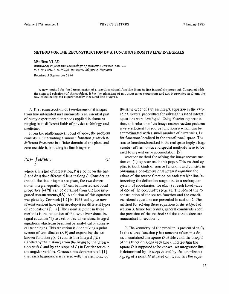
2. The geometry of the problem is presented in fig. 1: the source function g has nonzero values in a do-

main contained in a square D of side a and the integral of this function along each line L intersecting the square D is supposed to be known. An integration line is determined by, its slope m and by the coordinates x0, y. of a point M situated on it, and has the equa-

13

Volume 107A, number 1 PHYSICS LETTERS 7 January 1985

a

Fig. 1. The geometry of the problem.

tion:

Y=Yotm(X -x0). (2) The line integral of g&y) along the straight line L is

=(l tm2)‘+lxg(x,~o tm(x-x0)). (3)

This is the rectangular-coordinates formulation of eq. (1) and represents a two-dimensional equation for the function g(x,u). An equivalent one-dimensional inte- gral equation in which one of the variables of g is a parameter can be derived as follows. The first step is to sum up the line integrals of the function g divided by the factor (1 + m2)1/2 along all positive-slope, straight lines intersecting in a point M(x,, yo) exter-

nal to the square D. The result is a function F depend- ing on the coordinates x0, y. of the point M:

90/(x0-a)

F(xu> YO) = s jQI4, m)(l + m2)-l12drn . (4) 0

This function can be expressed as an integral in the range y <y. of the unknown function g multiplied by a factor independent of the coordinate y. In order to demonstrate this statement, expression (3) offlM,m) is substituted into (4) and a permutation of the two integrals is performed:

F(xo,Yo)~

a YolCco-a)

= dx s s dm g(x, YO + m(x - x0)) . (5) 0 0

The change of variable u = y. t m(x -x0) in the sec- ond integral leads to the desired result:

14

F(xo,yo) = j dx &u g(x. u)(xo -x)-l . (6) 0 0

Differentiating both sides of the last equation with respect toy0 one can see that the problem separates and an integral equation in the variable x for the func- tion g at a fixed value y. of y is obtained:

a

J dxg(x, Y&o -xl-’ = G(x,20) * (7) 0

The right-hand side term G(xO,yO) is determined by the line integrals flM, m) and is given by

rol(xo-a)

G(xo> yo) = s dm (1 t m2)-1:2 0

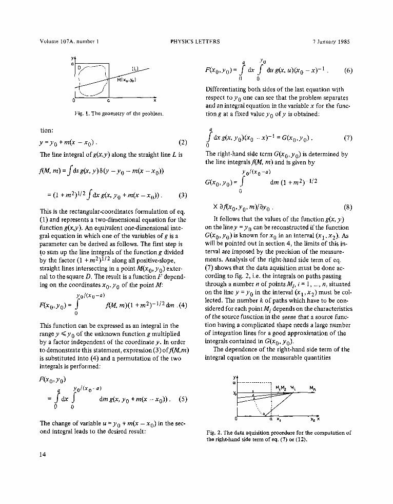
It follows that the values of the function g(x, y) on the liney = y. can be reconstructed if the function G(xo, yo) is known for x0 in an interval (XI, x2), As will be pointed out in section 4, the limits of this in- terval are imposed by the precision of the measure- ments. Analysis of the right-hand side term of eq.

(7) shows that the data aquisition must be done ac- cording to fig. 2, i.e. the integrals on paths passing through a number n of points Mi, i = 1, . . . . n, situated on the line y = y. in the interval (x 1, x2) must be col- lected. The number k of paths which have to be con- sidered for each point Mi depends on the characteristics of the source function in the sense that a source func- tion having a complicated shape needs a large number of integration lines for a good approximation of the integrals contained in G(xo, yo).

The dependence of the right-hand side term of the integral equation on the measurable quantities

Fig. 2. The data aquisition procedure for the computation of the right-hand side term of eq. (7) or (12).

Volume 107A. number 1 PHYSICS LETTERS 7 January 1985

flxo, Yo, m) can be simplified in the sense that the

derivative can be suppressed. This is done using the definition of the derivative with respect to Yo:

and observing that flxo, y. - h, m) can be replaced

by .f& + him yo, m) because they represent the integral of g along the same path. This yields

Mxo,Yo, W/dYo = --m-lW~xO,YO, mW0 , (10)

so that the function G(x,,Y,) becomes

vcl(xe-a)

G(XO,YO = s dm m-l(l + m2)-l12

0 x veo,yo, mYax . (11)

The limit of the integrand at m = 0 is given by

af(xO, y0, O)/ au0 and, in fact, it is independent of x0. The integration of both sides of eq. (7) with respect to x0 transforms it into the following equivalent equation:

(12)

u#J(xp)

&),Yo) = s dm m-l( 1 + m2)-1/2 0

X vTxl;yo, m) -f(~O,yO, m)l . (13)

3. The one-dimensional integral equation (7) or (12) for a section through the function g is a Fredholm type, first kind integral equation in the variable x Cyo is just a parameter). This kind of equations (and especially those having smooth, slowly varying kernels like (7) or (12)) are “ill-posed” problems in the sense of Hadamard,

i.e. their solutions are not stable with repect to small varia- tions of the known functions. This is a consequence of the fact that a large-amplitude variation 6g of the func- tion g is transformed by the integral operator into an arbitrarily small variation 6G of G if it is sufficiently fast oscillating and, conversely, a small error 6G of G can correspond to arbitrarily large variations 6g of the computed solution g. Special numerical methods which prevent such oscillations were developed in the last pe- riod [8-121.

We have used for eq. (7) or (12) a least-squares tech- nique [8,10] which consists in finding a least-squares approximation of the solution which also minimises a smoothing functional of the form

where the prime denotes derivative with respect to x and ql(x), q2(x) are continuous, positive functions and represent weighting factors. A good choice of these factors is

41(x)=42(x) = 1/(x2 + 1) , (15) because the kernel of eq. (7) or (12) is characterised by a small variation in the first half of the interval (0, a),

followed by a large growth in the second half. As a con- sequence of this feature, the random error accumulation tends to be more important in the interval (0, a/2) than in the interval (a/2, a). The use of the weighting factors

(15) having larger values in the first part of the interval determines a preferred attenuation of the noise in the first part of the interval.

In order to obtain a high precision discretisation of the integral in the equation, the cubic B-spline represen- tation of the unknown function g was used. The linear algebraic system obtained from the minimisation condi- tion was solved by means of an iterative technique pro- vided by the conjugate gradient method [lo]. This method gives very good results for such ill-conditioned systems because it is not dealing with matrix inversions, being based only on matrix multiplication operations, The subroutines for the computation of the right-hand side term of eq. (12) from the experimental values of the line integrals use a smoothing and interpolation method also based on the spline function representation.

4. The method for solving the image reconstruction

problem was numerically tested using given source functions g and computing the line integrals by means of (2). The subroutines for determining the right-hand side term of eq. (12) were analysed separately by com- paring the& result with a direct, high precision compu- tation of G(x,, yo) from the left-hand side integral of eq. (12). For each kind of function g, the number k of line integrals which provides a good approximation of G(xo, yo) can be found in thjs way. Having the values of the right-hand side term G(x,,,_v~), i = l,..., n, eq.

15

Volume 107A, number 1 PHYSICS LETTERS 7 January 1985

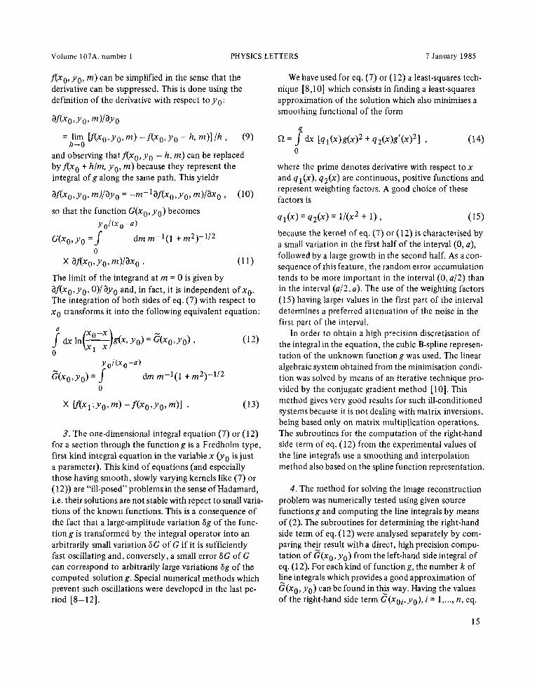
Fig. 3. The results obtained for the test function represented by the continuous line for different values of the parameters x1 and x2. The maximum relative errors in the right-hand side term of eq. (12) were determined to be: o: d G/G = 10e4%,xr = 1,5,X2 =2.;+:&G/G=10-2%,x1=1.2,x,=2.;x:&G/G=l%, xt = 1.05,x2 = 2.

(12) was solved by means of the stabilisation method and the computed solution was compared with the test function. Principally, the interval (xl, x2) of the varia- ble x0 is arbitrary but numerical experiments show that it depends on the level of errors in the right-hand side term of the equation in the sense that, for eachgiven in- terval, the solution can be obtained only if the level of errors is beyond some limit. This limit grows when x1 + a andx2 +=, the dependence onxl being stronger than that on x2. A test result is presentedin fig. 3. The maximum values of the random errors in G for which the test function (continuous line) can still be recon- structed are indicated for some values of the parameter x 1. There are no general analytical methods for deter- mining the dependence of the range of the variable x0 on the level of the experimental random errors but the numerical simulations described here can evaluate it, if a guess of the unknown function can be made.

It must be pointed out that this method can be used

for source functions which are characterised by a large maximum in a region D’ of the square D, making it pas-

sible to reconstruct details of the function out of this region from line integrals on paths which do not inter- sect D'. In Cormack’s method all the line integrals on paths situated at a distance r > r. from the origin are

involved in a value ofg at r = r. so that the small details of g are folded in the errors because line integrals of the large maximum are summed with line integrals of the small details. The particular mode of collecting the line integrals could also be of interest in radiological applica- tions making it possible to obtain the tomography of a part of a domain, protecting from radiations from some other part.

References

[l] A.M. Cormack, J. Appl. Phys. 34 (1963) 2722. [2] A.M. Cormack, J. Appl. Phys. 35 (1964) 2908. [3] N.R. Sauthoff and S. von Goeler, IEEE Trans. Plasma Sci.

PS-7 (1979) 141. [4] R.C. Chase and J.A. Stem, Med. Phys. 5 (1978) 497. [5] Z.H. Cho et al., IEEE Trans. Nucl. Sci. NS-22 (1975) 344. [ 61 P. Smeulders, Max Planck Institut fiir Plasmaphysik,

preprint IPP 2/252 (1983). [7] G.T. Herman, ed., Image reconstruction from projections,

Topics of applied physics 32 (Springer, Berlin, 1979). [ 81 A. Tichonov and V. Arsenine, Methodes de resolution de

problemes maI poses (MIR, Moscow, 1976). [9] J. Albrecht, Clausthal-ZeIlerfeld and L. Collatz, eds.,

Numerical treatment of integral equations, (Birkhiuser, Basel, 1980).

[lo] H.S. Hou and H.C. Andrews, IEEE Trans. Comput. C-26 (1977) 856.

[ll] St.W. Provencher, Comput. Phys. Commun.27 (1982) 213,229.

[ 121 M. Bertero, C. DeMol and G.A. Viano, Lecture notes in physics 85 (Springer, Berlin, 1978) p. 180.

16