Mesoscale eddies in the southern Gulf of California during summer:Characteristics and interaction with the wind stress

M. F. Lavín,1 Rubén Castro,2 Emilio Beier,1 and Victor M. Godínez1

Received 3 August 2012; revised 16 February 2013; accepted 18 February 2013; published 20 March 2013.

[1] The hydrodynamic characteristics of mesoscale eddies of the southern Gulf ofCalifornia are described from observations made in August 2004. Vertical profiles to~1000m were made with a conductivity-temperature-depth (CTD) probe with dissolvedoxygen and fluorescence sensors, and a lowered acoustic Doppler profiler. The foursampled eddies were aligned along the Gulf axis and had alternating sense of rotation. TheOkubo-Weiss parameter was used to calculate the eddy core radii, and it also revealed thatthe current field of almost all the sampled area was eddy dominated. The mean radii of theeddy cores varied between 32 and 36 km. Maximum surface velocities were 0.4–0.5m/s.The anticyclonic eddies were 500–700m deep, while the cyclones were 450–500m deep.The depression of the isolines associated with the anticyclonic eddies was ~100m at depthsbetween 200 and 400m; however, the thermocline/pycnocline, which spanned from ~20 to75m, was domed by ~10m. The cyclonic eddies lifted the isolines by ~70m at depthsabove 500m, but the isolines were flat above ~60m. This suggests that different dynamicsoperate in the layer above the strong and shallow pycnocline. In particular, the wind stresscurl can affect circulation and pycnocline topography and, therefore, the patterns thatappear in chlorophyll satellite images. In our case, the eddies were detectable in thoseimages because of the chlorophyll-enhanced streamers along their edges and, foranticyclones, probably because the chlorophyll maximum found at 40–50m depthwas domed following the pycnocline.

Citation: Lavı́n,M.F.,R.Castro, E. Beier, andV.M.Godı́nez (2013),Mesoscale eddies in the southernGulf ofCalifornia duringsummer: Characteristics and interaction with the wind stress, J. Geophys. Res. Oceans, 118, 1367–1381, doi:10.1002/jgrc.20132.

1. Introduction

[2] The surface dynamics and thermodynamics of the Gulfof California (GC) (Figure 1) have been extensively studiedin the seasonal time scale [Lavín and Marinone, 2003, andreferences therein]. While the seasonal circulation isimportant and well understood, satellite images and numeri-cal models of the Gulf suggest that mesoscale eddies withdiameters of ~70–120 km (GC width 120–160 km) arecommon in the southern Gulf; yet, they have not been directlystudied in detail.[3] The oldest direct observations of a mesoscale eddy in

the Southern Gulf of California (SGC) (Figure 1) were madein August 1978 [Emilsson and Alatorre, 1997], usingsurface drifters, a lowered Aanderaa current meter, and afew conductivity-temperature-depth (CTD) casts; a cyclonic

eddy of ~50 km radius and ~70m depth was found overFarallón basin (see basin names in Figure 1). The only laterhydrographic evidence of eddies in the SGC (by Fernández-Barajas et al. [1994] from February 1992 and by Figueroaet al. [2003] from March 1984) suggest a series ofgeostrophic eddies, 400–500m deep, with alternating senseof rotation along the SGC; however, their stations were verywide apart or were from single along-gulf lines of stations,so that details were missing or no information was providedon the lateral structure.[4] Satellite infrared and color images have shown that

mesoscale structures are common features of the surface layerof the SGC [Badán-Dangon et al., 1985; Pegau et al., 2002;Navarro-Olache et al., 2004; Lavín and Marinone, 2003].Using sea-viewing wide field-of-view sensor, ocean colorimages from early September 1999, Pegau et al. [2002]suggested that the surface circulation during late summer inthe SGC was dominated by eddies, with alternating sense ofrotation, with radii of ~35–50 km. The presence of an eddypair extending from Cabo Lobos (Figure 1) in three consecu-tive years suggested to these authors that the eddies weretopographically locked. However, this study was based solelyon satellite-derived chlorophyll pigment with no quantitativevalues, and there is no confirmation that the features theyobserved were actual deep eddies.[5] The generation of the SGC eddies was investigated

numerically by Zamudio et al. [2008] with a 3-D 1/12�

All supporting information may be found in the online version ofthis article.

1Centro de Investigación Científica y de Educación Superior deEnsenada, Ensenada, Mexico.

2Facultad de Ciencias Marinas, Universidad Autónoma de BajaCalifornia, Ensenada, Mexico.

Corresponding author: R. Castro, Facultad de Ciencias Marinas,Universidad Autónoma de Baja California, Carretera Tijuana-Ensenadakm 107, Ensenada, B. C. 22860, Mexico. (rcastro@uabc.edu.mx)

©2013. American Geophysical Union. All Rights Reserved.2169-9275/13/10.1002/jgrc.20132

1367

JOURNAL OF GEOPHYSICAL RESEARCH: OCEANS, VOL. 118, 1367–1381, doi:10.1002/jgrc.20132, 2013

nested interannual-forced regional Gulf of California hybridcoordinate ocean model, with local and/or remote forcing,that was nested in basin-scale and global models. Theyfound that remote forcing is essential for the generation ofeddies in the SGC. The simulations show that the interactionof the poleward Mexican Coastal Current with specifictopographic irregularities (capes at Topolobampo and CaboLobos, and the shelf ridge off the San Lorenzo River) couldgenerate eddies by inducing baroclinic instabilities and thatthis mechanism is strengthened by the arrival of coastal-trapped waves of equatorial origin. They also concludedthat local wind forcing was not essential for the generationof these eddies. In this model, the lifetime of the eddies is2–3months (August–October).

[6] The available evidence suggests that mesoscale eddiesare a very important (if not the most important) componentof the GC circulation during summer; yet, their physicalcharacteristics have not been described in detail. It is likelythat eddies have a role in the transport/retention of chemicalproperties and of planktonic organisms and in the redistribu-tion and mixing of properties at different levels of the watercolumn. Therefore, it is important to provide a quantitativedescription of relevant characteristics of the eddies (such asradii, depths, swirl velocities, Rossby numbers, vorticity,dynamic height anomalies, etc.) that can be used by numer-ical modelers and other observationalists. Tidal currents areweak (<0.05m/s) in the SGC [Marinone and Lavín, 2005]and are not considered here.[7] The objective of this study is to describe the hydro-

graphic and kinematic characteristics of the mesoscaleeddies of the Southern Gulf of California, based on highlydetailed direct observations [CTD and lowered acousticDoppler current profiler (LADCP)] made in August 2004.After describing data and methods in section 2, results(section 3) are presented of (a) the horizontal structure ofeddy currents and hydrography, (b) the vertical structure ofa representative anticyclone and cyclone, and (c) eddiesand chlorophyll images. The discussion (section 4) dealswith eddy dimensions and position, with the potential roleof the wind stress curl on near-surface dynamics and chloro-phyll images, with hydrographic structure, and with compar-ison of geostrophic velocity versus LADCP observations.

2. Data and Methods

[8] Hydrographic observations were made during cruiseNAME-2, carried out from 7 to 20 August 2004, on boardthe R/V Francisco de Ulloa, covering a large part of theSGC with a total of 196 oceanographic stations in 11across-gulf lines (Figure 1). The spacing between stationswas ~10 km in the across-gulf transects, and the along-gulfdistance between lines was between 30 and 40 km. Thissampling scheme was a compromise between fine across-gulf sampling and ample along-gulf coverage; the sectionscrossing near eddy centers provided good individual charac-terizations, while the other lines provided between-eddiesinformation that helped complete the description of the eddyfield. The width of the Gulf decreases from 180 km at linesA and B to 130 km at line F (Figure 1).[9] Temperature and conductivity profiles down to

1000m (or near the bottom if shallower) were measuredwith a factory-calibrated CTD (SeaBird SBE-911 plus), withprimary and secondary sensors and a sampling rate of 24Hz.Dissolved oxygen (DO, mL/L) and fluorescence sensors(SBE43 and SeaPoint, respectively) were also included.The fluorescence sensor had a range of 0–150mg/m3 ofchlorophyll a (abbreviated chl-a; mg/m3) and a 1� gain.The data were processed and averaged to 1 db as docu-mented by Castro et al. [2006]. Salinity was calculatedwith the Practical Salinity Scale (1978). Potential tempera-ture (θ, �C) and potential density anomaly (gθ, kg/m

3) werecalculated according to UNESCO [1991]. Geostrophicvelocity (VG, m/s) was computed using the deepest commondepth as reference level, which was ~1000m for most pairsof stations. Prior to geostrophic velocity calculation, thetemperature and salinity cross sections were objectively

E

Z

X

B

C

D

F

GH

I

A

Topolobampo

Cabo LobosGB

CB

FB

PB

Pacific Ocean

Cerralvo I.

La Paz BaySan Jose I.

Carmen I.

116°W

28°N

114°W26°N

24°N

112°W

|22°N

110°

W

108°

W

106°

W

30°N32°N

500

1000

1500

2000

2500

3000

3500

Depth (m)

USA

Mexico

Gul

f of C

alif

orni

a

Pacific Ocean

BA

JA C

AL

IFO

RN

IA P

EN

INSU

LA

Figure 1. Chart showing location of the hydrographicstations (•) during 7–20 August 2004. The names of the sectionsare included close to the mainland coast. The rough positions ofbasins are indicated as follows: GB=Guaymas basin, CB=Carmen basin, FB=Farallón basin, and PB=Pescadero basin.

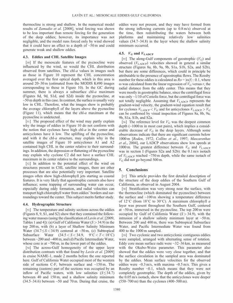
LAVÍN ET AL.: MESOSCALE EDDIES GULF CALIFORNIA

1368

mapped in order to remove internal waves and other small-scale variability. A standard objective mapping interpolationwas used, with a classical Gaussian correlation function withrelative errors of 0.1, with a 70 km horizontal length scaleand a 30m vertical scale. The chosen horizontal scale is abouttwice the baroclinic radius of deformation, which for ourregion is ~40 km [Chelton et al., 1998] (http://www-po.coas.oregonstate.edu/research/po/research/rossby_radius/index.html),thus ensuring that the smoothed sections resolve geostrophicflow. In addition, following Chereskin and Trunnell [1996],we computed the covariance of temperature and density datafrom the cruise for the 0–10 and 250–300m layers; a guesscorrelation of the covariance using a Gaussian functionresulted in length scales of ~70 km. Objective mappingwas also applied to the horizontal distributions, with scales0.3� of latitude by 0.3� of longitude.[10] Velocity profiles were measured with a broadband

Teledyne-RDI 300 kHz lowered acoustic Doppler currentprofiler (LADCP) attached to the CTD protection frame.The absolute velocity profiles were obtained with themethods described by Visbeck [2002]. The sampling bins

were 8m thick. Objective analysis was also applied to theLADCP velocity components with horizontal scale of70 km and 50m in the vertical. The covariance at 8–48 and248–304 layers was also computed for velocity components;the correlation length scale resulted ~30–40 km of the orderof the Rossby radius of deformation. We also used 70 km toreduce ageostrophic noise in the LADCP observations[Chereskin and Trunnell, 1996].[11] The horizontal distribution of LADCP velocities was

used to calculate the vertical component of relative vorticity

B ¼ @v

@v� @u

@y

and the Okubo-Weiss parameter W [Okubo, 1970;Weiss, 1991], which identifies regions where z dominatesover strain

W ¼ S2n þ S2s � B2

where Sn and Ss are the normal and shear components ofthe strain

0.2

0.2

0.2

0.2

0.2

0.2

0.2

0.2

0.2

0.2

0.3

0.3

0.3

0.3

0.3

0.4

0.4

0.4

0.40.5

Figure 2. Horizontal distribution of (a) average velocity (m/s) vectors from LADCP in the 8–48m layer(7–20 August 2004). Tracks and velocity vectors for drifters 50012 (blue) from 7 June to 19 August and50021 (red) from 20 July to 31 September are included. (b) Speed of currents from LADCP and, in red, thecontour W = 0. The following parameters were calculated with the velocity field. (c) The Okubo–Weissparameter, divided by the standard deviation of W in the area under observation (sw = 1.17� 10�10 s�2),with the thick black line marking W = 0 and the thin line marking W/sw = 0.2. (d) Relative vorticity(10�5 s�1) and, in red, the contour W= 0.

LAVÍN ET AL.: MESOSCALE EDDIES GULF CALIFORNIA

1369

Sn ¼ @u

@x� @v

@y; Ss ¼ @v

@xþ @u

@y:

[12] In areas where vorticity dominates the current field,W< 0, and in those where strain dominates, W> 0.When the flow field is partitioned with W, it is observed[Isern-Fontanet et al., 2004; Henson and Thomas, 2008]that eddies have a central area (the eddy core) where W isstrongly negative, surrounded by an area (the eddy ring orcirculation cell) where W> 0. The eddy core edge can bechosen as the connected curve where W = 0 or as the narrowclosed strip area where�0.2sw ≤W ≤ 0.2sw, where sw is thestandard deviation of W in the area under observation. Theouter eddy boundary is sometimes chosen as the line wherez = 0 [e.g., Kurian et al., 2011]. Beyond the eddy boundary,the background flow is usually characterized by small posi-tive and negative values of W (|W/sw| ≤ 0.2).[13] The Rossby number in polar coordinates is Ro = |

Centrifugal force/Coriolis force| = |V/fr|, where V is thetangential velocity, f is the Coriolis parameter, and r is radialdistance from the eddy center [e.g., Takahashi et al., 2007].Assuming that the eddy core rotates as a solid body, theswirl velocity and the angular frequency are related by

V=or, and o can be obtained from linear regression betweenV versus r for data points inside the eddy core. Then Ro= |o/f|.[14] Wind data with a horizontal resolution of 0.25� � 0.25�

and sampled every 6 h were obtained from the product called“Cross-Calibrated Multiplatform (CCMP) Ocean SurfaceWindVelocity Product forMeteorological andOceanographicApplications” [Atlas et al., 2011; ftp://podaac-ftp.jpl.nasa.gov/OceanWinds/ccmp/L3.0]. Wind stress and wind stress curlwere calculated from these data. Three-day mean satelliteimages (4� 4 km) of surface chlorophyll concentration fromtheMODIS satellites were obtained for 7, 9, 11, and 17August2004 (http://oceancolor.gsfc.nasa.gov/cgi/level3.pl). For thosedates, the MODIS K490 images were used to estimate thedepth of the first optical depth, as the inverse of the diffuseattenuation coefficient at 490 nm wavelength.[15] Surface currents were measured with two PacificGyre

(http://www.pacificgyre.com) SVP ARGOS drifters equippedwith holey socks centered at 15m. The drifters were deployedfrom the R/V Francisco de Ulloa during a cruise (NAME-1)made from 5 to 18 June 2004.The data were cleaned and inter-polated at 6 h intervals as described by Hansen and Poulain[1996]. The first drifter (No. 50021) sampled in the open Gulffrom 19 July to 31 August 2004. The other drifter (No. 50012)sampled from 7 June to 19 August 2004.

0.1

0.1

0.1

0.1

0.1

0.1 0.1

0.1

0.1

0.1

0.1

0.1

0.1

0.1

0.1

0.10.1

0.2

0.2 0.2

0.2

0.2

0.2

0.2

Figure 3. Same as Figure 2 but for the 248–298m LADCP velocity layer.

LAVÍN ET AL.: MESOSCALE EDDIES GULF CALIFORNIA

1370

3. Results

3.1. Eddy Currents: Horizontal Structure

[16] The horizontal distribution of drifter and LADCPsurface current vectors (8–48m vertically averaged LADCPdata) (Figure 2a) shows four eddies distributed along thesouthern Gulf, with alternating sense of rotation, namely(from the mouth to the head of the gulf): anticyclonic eddyA1, cyclonic eddy C1, anticyclonic eddy A2, and cycloniceddy C2. Mean velocity magnitudes around the eddies(Figure 2b) were ~0.3m/s, with maxima ~0.4–0.5m/s incertain spots, especially where eddies interacted. The eddieswere so close to each other that their respective current fieldscannot be told apart by looking at Figure 2a.[17] The surface distribution of W/sw (Figure 2c) calcu-

lated from the LADCP data shows that the main eddies wereslightly elongated in the approximate direction of the gulfaxis (NW-SE), except for A1, which was elongated in theN-S direction. The major and minor semiaxes for the eddycores (where W = 0) are as follows: A1, 32 and 39 km; C1,27 and 40 km; and A2, 27 and 38 km. There appearedanother weak eddy southeast of A1, not evident in Figure 2a,but its W/sw and speed were lower than for the other eddies.Outside the eddy cores, W/sw was positive with maximumW/sw= 1 (where, in this case, sw= 1.17� 10�10 s�2). Thisvalue of W/sw is slightly smaller than in typical areassurrounding eddy cores (1.5–2) [Isern-Fontanet et al., 2004].

Away from the eddies, |W| falls below 0.2sw in very fewplaces (especially in the SE), which means that there was verylittle background area or that almost the entire sampled areawas affected by the eddies. The surface relative vorticity field(Figure 2d), computed from the LADCP (8–48m layervelocity field), defined very clearly eddies A1, C1, and A2(not C2, because it was sampled by a single line of stations).The boundaries between eddies cannot be established withthe velocity field nor with the distribution of W, but we candefine them as the contour z= 0; the area between the contoursW=0 and z= 0 (Figure 2c) would be the “eddy ring” or the“circulation cell.” The core radii were not much smaller thanthose of the eddy rings, probably because the eddies were soclose to each other.[18] Eddy A1 (Figure 2) covered part of Pescadero basin.

Its mean core radius was 36 km, and its highest speeds(~0.5m/s) were at its eastern margin. Off the peninsula,speeds were between 0.2 and 0.3m/s. The red drifter(50021) showed a slow (~0.13m/s average) northwarddisplacement across the position of A1, from 7 to 25 June2004, which suggests that A1 was probably formed in July.In the surface layer (Figure 2d), A1 had the maximumnegative relative vorticity (�2� 10�5 s�1), while the meanvalue inside the W=0 contour was �1.38� 10�5 s�1.[19] Cyclonic eddy C1 (Figures 2a and 2b) was located

northeast of Bahía de La Paz, and it occupied much ofFarallón basin. Its mean swirl speed was ~0.30m/s along

Figure 4. Horizontal distribution at upper 10m: (a) temperature (�C), (b) salinity, (c) density anomaly(kg/m3), and (d) dissolved oxygen (mL/L) during the cruise, 7–20 August 2004.

LAVÍN ET AL.: MESOSCALE EDDIES GULF CALIFORNIA

1371

its edge (with a maximum over 0.40m/s in the SW side), andits mean core radius was ~33 km. The drifter data suggestthat eddy C1 was present at least since late June. The trajec-tory of the blue drifter between 26 and 29 June was towardthe east in section D, and then it veered north, probablyfollowing the southern and eastern edges of the eddy. From4 to 14 July, it completed a loop around C1 (~30 km radius)with a mean velocity of ~0.21m/s. From 19 to 26 July, itmade another smaller cyclonic loop inside C1 (~14 kmradius, 0.20m/s mean velocity). The red drifter, which on20 July was outside La Paz Bay, roughly followed the southernand eastern edges of the eddy until 28 July, at ~0.28m/s.C1 had a mean vorticity in the eddy core of 1.49� 10�5 s�1

and a maximum positive vorticity of ~2� 10�5 s�1.[20] Eddy A2 was located around ~26�N (Figure 2),

almost centered on Carmen basin. The highest speeds werefound in the southern edge (where it interacted with C1),where they ranged between 0.3 and 0.4m/s. The mean coreradius was ~33 km. The presence of A2 was also revealed bythe tracks of both drifters, which followed its westernand northern edges. The blue drifter showed speeds of~0.20m/s (from 29 July to 4 August), and the red drifter(50021) had an average speed of ~0.30m/s (from 28 Julyto 3 August). The vorticity of A2 was relatively lower thanthat of A1 (Figure 2d), with a mean value of �1.1� 10�5

s�1 in the eddy core and a maximum of ~�1.5� 10�5 s�1.

[21] Cyclonic eddy C2, located on Guaymas basin, wassampled with North-South section I (Figure 2a), which wasa last-minute change in the cruise plan when the presenceof this eddy became apparent in drifter tracks and satellitechlorophyll images. The radius of C2 was ~32 km, and themaximum (LADCP) velocities were ~0.4m/s. This eddywas well sampled by the drifters. The blue drifter loopedonce around C2 with speed ~0.27m/s, in a radius ~37 km,taking 12 days (7–19 August) to complete the loop. Thered drifter, after drifting toward the NW (0.5–0.40m/s; mean~0.20m/s) approximately parallel to the mainland coast,veered west off Cabo Lobos and made three loops aroundeddy C2 with ~30 km mean radius, between 7 Augustand 4 September, with mean speed ~0.33m/s (range:0.09–0.58m/s) and rotation period between 6 and 9 days.Other drifters (not shown) trapped in this eddy showedthat it lasted at least until October 2004.[22] In general, the pattern of currents in the 248–304m

layer did not change much relative to the surface layer,although their speed decreased with depth (Figures 3a and3b; note the change of scale relative to Figures 2a and 2b).The fastest currents (Figure 3b) were in the area of interac-tion between C1 and A1. The eddies had lower absolutevalues of W and vorticity (Figures 3c and 3d), but the coreswere larger and more elongated than at the surface. The W=0and z =0 contours were quite close.

Figure 5. Horizontal distribution at 300m: (a) temperature (�C), (b) salinity, (c) density anomaly (kg/m3),and (d) dissolved oxygen (mL/L) during the cruise, 7–20 August 2004.

LAVÍN ET AL.: MESOSCALE EDDIES GULF CALIFORNIA

1372

3.2. Horizontal Hydrographic Structure

[23] Figure 4 shows the horizontal distributions of poten-tial temperature (θ), salinity (S), potential density anomaly(gθ), and DO concentration, averaged over the 0–10m layer.The train of eddies described above based on current datawas not apparent in the surface hydrographic variables. Thisis due to the relative homogeneity of the properties of thesurface layer of the SGC. Surface temperature (Figure 4a)was lower close to the peninsula (~28�C –29�C) than thatoff the mainland coast (29.5�C–31�C). A nucleus with tem-perature lower than 30�C appeared around 24.5�N–109�W,but it does not seem to be associated to any cyclonic eddy.The salinity distribution showed an overall latitudinal gradi-ent increasing from south to north (Figure 4b); low values

(34.6–34.7) were observed at the center of the Gulf entrance(sections Z-X) and close to the mainland coast (34.7–34.8).The 35.0 isohaline apparently marked the boundary betweenGulf of California Water and Pacific waters and was shapedlike a tongue between sections C and A-X. The maximumvalues (35.3–35.4) were located in the northern part of theobserved region, between sections H and I. gθ showed a gradi-ent similar to that of θ but reversed (Figure 4c), with highvalues (~22 kg/m3) close to the peninsula and low values onthe mainland coast (21.3–21.4 kg/m3). The surface DOconcentration (Figure 4d) was homogeneous, at ~4.4mL/L,with an increase to 4.6mL/L off themainland in the gulf mouth.[24] In contrast to the lack of evidence of the eddies’

presence in the surface properties of Figure 4, the horizontaldistribution of hydrographic variables at 300m (Figure 5)was clearly influenced by the eddy train, being characterizedby well-defined cores with concentric circular isolines aroundrelative maxima or minima. Anticyclonic eddies A1 and A2

Figure 6. Depth of potential isopycnal anomaly surfaces:(a) 26.5 kg/m3 and (b) 27.2 kg/m3.

Figure 7. Dynamic height anomaly: (a) 100m relative to500m and (b) surface relative to 500m.

LAVÍN ET AL.: MESOSCALE EDDIES GULF CALIFORNIA

1373

were marked by cores that, relative to the surroundings,were warm (12�C and 12.5�C, respectively), salty (34.8and 34.85), and with relatively high DO content (0.5 and0.8mL/L). The core of cyclonic eddy C1 was relatively cold(10.5�C), less saline (34.7) and with a lower DO content(~0.25mL/L) than the surroundings; no concentric isolinesof DO were apparent because the values of this variable werevery low below the oxycline. The density anomaly contours(Figure 5c) were similar to those of temperature, with lower

values (26.45–26.4 kg/m3) in the core of anticyclonic eddiesand higher values (26.55 kg/m3) in cyclonic eddy C1.[25] The descriptions above are congruent with the lifting

of deep (deeper than ~300m) isolines in cyclones anddeepening in anticyclones. The magnitude of the verticaldistortion of the deep isolines is illustrated by the topogra-phy of the 26.5 and 27.2 kg/m3 isopycnal surfaces (Figure 6).The vertical distortions of the 26.5 kg/m3 surface (Figure 6a)had amplitude ~120m, with maximum depth (~350m) in

Figure 8. Vertical structure across-Gulf for section C: (a) geostrophic velocity (m/s) using the deepestcommon depth for two adjacent stations as a reference level, (b) velocity component perpendicular tothe section (VLADCP, m/s), (c) potential temperature (�C), (d) density anomaly (kg/m3) and fluorescence(mg/m3), (e) salinity, and (f) dissolved oxygen (mL/L). Positive (negative) values of velocities indicateinflow to (outflow from) the Gulf. In Figures 8c–8f, the horizontal line at 200m indicates the change invertical scale: the upper 200m are stretched, so that the structure of the upper layers can be appreciated.

LAVÍN ET AL.: MESOSCALE EDDIES GULF CALIFORNIA

1374

anticyclones A1 and A2 and minimum (~230m) in cycloneC1. The distortions were smaller (~50m) for the 27.2 kg/m3

isopycnal surface, with depths between 730 and 740m forA1 and A2 and 680m for C1. The center of eddies C1 andA2 seems to be shifted southward with depth (Figure 6b).[26] To obtain an idea of the scale of the surface distortion

associated to the eddies, we calculated the dynamic height(m) as geopotential anomaly/g and then estimated the anom-alies by dividing by the average over the sampled area. Thiswas done for the surface and for 100m (to avoid near-surface effects), relative to 500m. At 100m, (Figure 7a),the maximum elevation at A1 was ~4 cm, C1 had a depres-sion of �2 cm, and A2 had an elevation of 4 cm. The surfacedynamic height anomaly relative to 500m (Figure 7b) showsthat the shape of C1 was similar to that in Figure 7a but with

a maximum depression of 5–6 cm. Substantial changes ofshape are apparent for anticyclones A1 (anomaly ~5–6 cm)and A2 (anomaly ~2 cm), compared to those in Figure 7a;this reflects the effect of the pycnocline topography, whichis found above ~75m, and is probably strongly affected bythe wind, as will be discussed later.

3.3. Vertical Structure of Eddies

[27] Vertical sections across eddies were selected todescribe their circulation and hydrography (see sectionpositions in Figure 2): section C for anticyclonic eddy A1(Figure 8), section H for eddy A2 (see Figure S1 inthe Supporting Information), section F for cyclonic eddy C1(Figure 9), and section I for eddy C2 (Figure S2). Only oneanticyclone (A1) and one cyclone (C1) are described here;

Figure 9. Same as Figure 8 but section F.

LAVÍN ET AL.: MESOSCALE EDDIES GULF CALIFORNIA

1375

the graphs corresponding to A2 and C2 are found in theSupporting Information. Note the stretching of the verticalscale above 200m in Figures 8c–8f and 9c–9f to better showthe structure of the upper layers.3.3.1. Anticyclonic Eddy A1 (Section C)[28] The speed across section C (eddy A1) calculated by

geostrophic balance (VG, Figure 8a) and measured withLADCP (VLADCP, Figure 8b) show similar structures, withinflow on the peninsula side and outflow spanning thecentral and eastern parts of the section. The VG inflow(Figure 8a) was ~50 km wide and ~700m deep, with speedmaximum (0.2m/s) between 100 and 300m. The VG outflowwas ~65 km wide and ~700m deep; the 0.2m/s isotachreached ~300m and the 0.25m/s reached 200m, with themaximum (~0.35m/s) at the surface and at a core at~100m depth. The VLADCP inflow (Figure 8b) adjacent tothe peninsula was faster (maximum ~0.35m/s) than the VG

inflow (maximum ~0.25m/s); the core of maximum speedwas between 200 and 350m, while speeds ~0.10m/s werefound at ~600m. The VLADCP outflow was weaker than theVG outflow; maximum VLADCP outflow speeds (~0. 25m/s)were above 100m. On the mainland shelf, a shallow inflow(above 50m) was also observed, with VG speeds between0.10 and 0.15m/s.[29] The vertical sections of potential temperature (θ),

potential density anomaly (gθ), salinity, and DO across eddyA1 (Figures 8c–8f) show, below ~200m, a central depres-sion of the isolines. The depressions diminished with depthbut were noticeable down to ~700m. Almost no sidewayshift with depth was exhibited by the center of the depres-sion. The 11�C isotherm (Figure 8c) sank from ~290m overthe mainland slope to a depth of ~400m at its maximumdepth. The 26.5 kg/m3 isopycnal deepened from ~260m

over the slope to a depth of 350m at its maximum depth(Figure 8d). The depression of the 1.5–0.5mL/L DO isolines(Figure 8f) were located at a distance of 50 km from thepeninsula and positioned on the west side of the section;the 1mL/L isoline sank from ~140 to 240m, whereas the0.5mL/L isoline reached ~310m. The minimum oxygenzone (≤0.1mL/L) was distributed between 400 and 850m.[30] In the upper 150m of A1, isolines of temperature,

salinity, density, and DO were not concave but slightlyconvex (Figures 8c–8f), especially in the top 70m. Clear con-vexity was exhibited by the thermocline, that is, by isotherms18�C to 28�C. The pycnocline (25–22 kg/m3, Figure 9d) andthe oxycline (4.5–2.0mL/L, Figure 8f) also showed slightdoming. The near-surface dome shape of the pycnoclinecaused VG to diminish above ~75m, producing the VG inflowmaximum at 150–300m depth (Figure 8a).[31] The distribution of chlorophyll a (chl-a, color

Figure 8d) presented a maximum (0.6–0.9mg/m3) in thepycnocline and values <0.2mg/m3 in the 20m below thesurface. The maximum values of chl-a in the thermoclinewere at the edges of the section (Figure 8d).[32] Salinity above 200m depth (Figure 8e) was structured

in three layers: (1) a surface layer (<40m) with the highestsalinities (34.9–35.1); (2) a shallow relative minimum layerwith salinity 34.7–34.8 between ~40 and 100m depth [thislayer was thicker (~85m) and relatively fresher in the westernhalf of the section]; and (3) a subsurface layer of relativelyhigh salinity (34.9–35.0) between ~70 and 230m, with a35 km wide core of S=35.0 between 110 and 150m depth.Dissolved oxygen (Figure 8f) showed a homogeneous layer(4–4.5mL/L) between 0 and 40m and strong stratification(2.5–4mL/L) between ~40 and 70m (Figure 8d).3.3.2. Cyclonic Eddy C1 (Section F)[33] TheVG distribution across cyclonic eddyC1 (Figure 9a)

shows that it was ~550m deep, was centered on the section,and had maximum speed ~0.25m/s in the outflow and~0.30m/s in the inflow; both maxima were at or very closeto the surface. The inflow shows an extension toward themainland continental shelf (maximum VG ~0.45m/s). Thecyclonic flow pattern shown by VLADCP had a structure inthe inflow similar to that of VG but deeper (~650m), withmaximum velocities (~0.25m/s) between 0 and 300m. Theoutflow maximum velocities (~0.20m/s) occurred between0 and 100m.[34] The isotherms and isopycnals in section F (Figures 9c

and 9d) presented doming in the central part of the sectionfrom ~700m and up to ~60m. The maximum lifting ofisotherms (~75m) occurred between 150 and 350m (Figure 9a).In the upper 50m of the water column, the isotherms andisopycnals present a slight downward tilt toward the mainland.Chl-a (color, Figure 9d) was maximum (0.6–0.8mg/m3) onthe pycnocline at ~40m; there was a surface layer with<0.2mg/m3 of chl-a in most of the section, except in themainland side, where it exceeded this value.[35] The upper salinity distribution in section F was

arranged in three layers, like in eddies A1 and A2 (Figures 9eand S1e). The maximum salinities (34.9–35.2) occurred in a40m deep surface layer. There followed the ~20m thickshallow salinity minimum (<34.9), centered at 50m depth.The >34.9 salinity layer was domed and reached ~150mdepth in the center of the section. The DO isolines(Figure 9e) between 350 and 100m were domed. The depth

Figure 10. Three day average surface chlorophyll a image(mg/m3) centered on 9 August 2004. In order to show thatthe image features reflect the eddies, we overlaid the W= 0contour and the drifter trajectories.

LAVÍN ET AL.: MESOSCALE EDDIES GULF CALIFORNIA

1376

of the 1.0mL/L isoline ranged between 145 and 175m,and the minimum oxygen layer was found between 300and 800m.

3.4. Eddies and MODIS Chlorophyll Images

[36] The along-Gulf sea surface temperature homogeneityin the SGC (Figure 4a) precluded satellite detection of theeddies with that variable, but MODIS CHL images did showthem, in part due to the relatively high CHL filaments thatemerged from coastal points. This is shown in Figure 10,which shows the 3 day mean CHL image for 9 August. Toprove that the structures observed in the image correspondwith the eddies described above, the Okubo-Weiss parame-ter W= 0 contours and the drifter velocities are overlaidon the image.[37] The satellite CHL data at each CTD station were

highly correlated with the corresponding near-surface CTDchlorophyll a (Figure 11) when vertically averaged overthe top 20 and 30m, which are depths of the order of thefirst optical depth estimated from the corresponding

MODIS K490 image (not shown). Although the satelliteCHL values are slightly higher than those from the CTD,the main peaks and lows coincide very well; the correlationcoefficients were 0.85 and 0.82 for the 20 and 30maverages, respectively.[38] With the exception of the coastal band and an

offshore filament off the mainland at the entrance to the GC(Figure 10) with the maximum surface CHL (~1mg/m3),concentrations were low (0.1–0.25mg/m3), but contrasts weresufficient to reveal the eddies and filaments. These structureswere immersed in an overall surface CHL gradient increasingfrom ~0.1mg/m3 at the Gulf entrance to 0.25mg/m3

around the archipelago that contains the large islands ofTiburon and Angel de la Guarda, where tidal mixing is strong[Argote et al., 1995].[39] On 9 August (Figure 10), relatively high CLH

concentrations were observed over the north margins of C1and C2, where thin filaments of relative high CLH appearedto arc cyclonically from the mainland coast at ~25.7ºN(close to Topolobampo) and ~27ºN (close to Cabo Lobos).

Figure 11. Chlorophyll a concentrations (mg/m3) in the top layers of the southern Gulf of California inAugust 2004, along (from W to E) the lines of stations shown in Figure 12. Black line: three day averagesatellite data closest to the dates when the stations were made, from images centered on 7, 9, 11, and 17August; blue lines: average of the top 20m from the CTD fluorometer; red lines: average over the top 30mof the CTD fluorometer. The dots mark the position of the CTD stations.

LAVÍN ET AL.: MESOSCALE EDDIES GULF CALIFORNIA

1377

In anticyclones A1 and A2, relatively high CHL concentra-tions were present in the center of each eddy, which weremost evident in A1.

4. Discussion

4.1. Structure and Position

[40] The structure of the Southern Gulf of Californiamesoscale eddies is described here for the first time basedon detailed direct observations of currents and hydrographicproperties, made in August 2004. This is a much morethorough description than those made previously from directhydrographic observation [Fernández-Barajas et al., 1994;Figueroa et al., 2003], which did not have such detailedsampling. Four eddies were sampled, two anticyclones andtwo cyclones, arranged with alternating sense of rotation.Mean surface core radii were ~32–36 km (Figure 2 andTable 1); both anticyclones and cyclones had highsurface velocities, with mean speeds ~0.3m/s and maxima~0.4–0.5m/s. The depth of the eddies, given by the0.05m/s isotach, was 550–700m for anticyclones and400–500m for cyclones (Figures 8, 9, S1, and S2; Table 1).[41] Using the surface distributions of W=0 and z=0

(Figures 3c and 3d) to position the eddies relative to the ba-thymetry and coastal features (Figure 1), anticyclone A1covered part of Pescadero basin, centered slightly to the westside of the basin, while A2 was located roughly over Carmenbasin. Cyclone C1 occupied much of Farallón basin.Cyclonic eddy C2 was located south of Guaymas basinand north of Carmen basin.[42] The data of Fernández-Barajas et al. [1994] from a

single line of stations along the longitudinal axis of theSGC during February 1992 showed geostrophic velocitiesof alternating sign reaching ~1000m, suggesting thepresence of eddies similar to those reported here. However,their cyclonic eddy at Pescadero basin had a radius of~90–100 km, while the anticyclonic eddy between Carmenand Farallón basins was ~85 km in radius; both estimatesare much larger than ours. Their maximum surface speed(0.95m/s) was also much faster than in our observations,probably because they did not smooth the hydrographic dataprior to calculating geostrophic velocity. The sequenceof eddies described by Figueroa et al. [2003] hascharacteristics similar to ours, maximum speeds ~0.5m/sand ~500m deep.[43] The late summer eddies studied by Pegau et al. [2002]

from ocean color images of the SGC had radii ~35–50 km, andthey estimated maximum velocities ~0.32m/s, which issimilar to our measurements. In general, the locations ofthose eddies (anticyclones in Guaymas, Farallón, and south

Pescadero basins, and a cyclone in Carmen basin) are not inagreement with the ones reported here, which is notunexpected considering that Figueroa et al. [2003] foundno consistent patterns in the reported positions of mesoscaleeddies in the SGC.[44] Comparing our observations with the results of the

numerical model of Zamudio et al. [2008] for the dates ofthe survey (their Fig. 12e), the model showed an anticyclonecovering much of Pescadero basin but was approximatelytwo times larger than A1, which was located SW of thatbasin. The three remaining eddies were in roughly similarpositions but had senses of rotation inverse of thoseobserved directly. These discrepancies can be expected in anumerical model that did not include data assimilation.Compared with the observations, the model eddy radii(~33 km) were similar, the mean speed (>0.45m/s) wasslightly higher, and they were deeper (~1000m).[45] The origin of the SGC eddies is not fully understood,

although it has been proposed that they may be caused byinstabilities of the poleward Mexican Coastal Current (whichoutside the GC is ~400m deep) [Lavín et al., 2006], especiallyduring the passage of coastally trapped waves [Pegau et al.,2002; Zamudio et al., 2008].

4.2. Dynamics Above the Pycnocline

[46] One of the observed features of all the eddies reportedhere was that the isopycnals in the pycnocline (and otherisolines in that zone) did not have the same concavity asthe deeper ones. While the sense of rotation of theeddies was established by the concavity of the deeper(100–500/800m) isopycnals, domed for cyclones, anddepressed for anticyclones, the shallow pycnocline wasdomed in the anticyclones (Figures 8d and S1d) and flat inthe cyclones (Figures 9d and S2d). This caused the maxi-mum geostrophic velocity to tend to be under the pycnoclinefor anticyclones. The pycnocline in the SGC is very strongand shallow, covering from almost the surface to ~75mdepth (Figures 8, 9, S1, and S2). The effect of the topogra-phy of the strong and shallow pycnocline was also evidentwhen comparing the dynamic height (Figure 7) at 100mand the surface (both relative to 500m)[47] These results suggest that the dynamics of layers

above and in the pycnocline may be different from that ofthe layers below. A possible mechanism for producing theobserved pycnocline shape is the interaction of the windand the eddy surface current. Since the wind stress dependson the wind velocity relative to the ocean surface velocity,even a homogeneous wind can cause a wind stress curl whenblowing over eddies [Martin and Richards, 2001;McGillicuddy et al., 2007].

Table 1. Characteristics of Eddies in the Southern Gulf of California in the Summer of 2004, From CTD and LADCP Observationsa

EddySurface

Semiaxes [km] Depth [m]Range of Surface Speeds

at Maximum [m/s]Maximum SurfaceVorticity [10�5 s�1]

Mean SurfaceVorticity [10�5 s�1]

A1 32� 39 700–800 0.25–0.5 �2 �1.4 (�1.45f)C1 27� 40 400–500 0.3–0.45 2 1.5 (1.51f)A2 27� 38 550 0.3–0.4 �1.5 �1.1 (�1.09f)C2 32 450 (VG) 0.3–0.4

700 (VAD)

aThe surface radii are the minor and major radii of the zero-value closed curves of the Okubo-Weiss parameter, that is, the “eddy core.” The mean surfacevorticity is the average inside the eddy core.

LAVÍN ET AL.: MESOSCALE EDDIES GULF CALIFORNIA

1378

[48] This was investigated by calculating the wind stress(t) with the formula

t ¼ raCD W � Vj j W � Vð Þ

where ra is the air density, CD is the drag coefficient asdefined by Large and Pond [1981] and modified byTrenberth et al. [1990], W is the average of the CCMP dailywind during the period of observations and interpolated tothe cruise stations by objective analysis (Figure 12a), andV is the surface current velocity. The time scale of the sur-face velocity field is mainly imposed by the geostrophicdeep eddies, so that the 18 days used for averaging the windshould be appropriate for calculating the wind stress, includ-ing the effect of the surface current. The wind variabilityellipses (Figure 12a), which were constructed from the stan-dard deviation of the wind components during the 18 days,have smaller major semiaxes than the mean value, and theellipses are approximately oriented in the direction of theaverage wind vector (N-NW). The wind stress curl assumingno water surface motion (V= 0) (Figure 12b) shows positive

curl (upwelling) in the peninsular half and negative curl(downwelling) in the mainland half of the GC. Eddies A1and A2 were in the upwelling area and C1 in a downwellingarea. The distribution of wind stress curl taking V from theobserved LADCP surface currents (V=VLADCP) (Figure 12c)shows a similar overall pattern, but it has a more markedmesoscale structure than with V= 0 (Figure 12b), and someof that structure reflects the effect of the eddies. This isclearer in Figure 13d, which shows the difference betweenthe two wind stress curl distributions. The intense positivecurl over anticyclonic eddies A1 and A2 will produceupward Ekman pumping and, therefore, a domed thermo-cline, as observed in Figures 8b and S2b. The negative curlover cyclonic eddy C1 would tend to depress or flatten thethermocline, as shown in Figures 9b and S2b. Therefore,the mesoscale features of the pycnocline topography maybe affected by the wind.[49] Beyond the possible effect of the wind on these

particular eddies, this leads to a wider consideration of thewind as an important forcing agent for currents in the upperlayers of the SGC, at least during summer when the

Figure 12. (a) Average of daily CCMP wind velocity vectors (m/s) for 18 days covering the period ofobservations and interpolated to the station positions using objective analysis. The variability ellipses(in red, 1 in 3 shown) were calculated from the standard deviation of the wind velocity components; minoraxes are shown as a red line. Wind stress (N/m2) was calculated using the formula t= raCD|W�V|(W�V),where ra is the air density, CD is the drag coefficient, W is the wind velocity from CCMP, and V issurface current velocity from LADCP. (b) Wind stress curl (N/m3) with V= 0. (c) Wind stress curl withV=VLADCP (blue arrows). (d) Difference between the two wind stress curl distributions.

LAVÍN ET AL.: MESOSCALE EDDIES GULF CALIFORNIA

1379

thermocline is strong and shallow. In the numerical modelresults of Zamudio et al. [2008], wind forcing was shownto be less important than remote forcing for the generationof the deep eddies; however, its importance was notnegligible, and the model runs forced only by wind showedthat it could have an effect to a depth of ~50m and couldgenerate weak and shallow eddies.

4.3. Eddies and CHL Satellite Images

[50] If the mesoscale features of the pycnocline wereinfluenced by the wind, so would the CHL distributionobserved from satellites. The chl-a values in images suchas those in Figure 10 represent the CHL concentrationaveraged over the first optical depth, which in this area isaround 20–30m (estimated from the MODIS K490 imagescorresponding to those in Figure 10). In the GC duringsummer, there is always a subsurface chl-a maximum(Figures 8d, 9d, S1d, and S2d) inside the pycnocline, at~50m depth in this case. In contrast, the surface is usually verylow in CHL. Therefore, what the images show is probablythe average chlorophyll of the layers above the pycnocline(Figure 11), which means that the chl-a maximum at thepycnocline is undetected.[51] The proposed effect of the wind may partly explain

why the image of eddies in Figure 10 do not conform withthe notion that cyclones have high chl-a in the center andanticyclones have it low. The uplifting of the pycnocline,and with it the chl-a structure, may explain why in thesatellite images of Figure 10 anticyclones A1 and A2contained high CHL in the center relative to their surround-ings. In addition, the depression or flattening of the pycnoclinemay explain why cyclone C2 did not have a surface CHLmaximum in its center relative to the surroundings.[52] In addition to the potential effect of the wind on

structures present in CHL satellite images, there are otherprocesses that are also potentially very important. Satelliteimages often show high-chlorophyll jets starting as coastalfeatures. It is very likely that ageostrophic currents also haveinfluence; some trapping of surrounding water can occur,especially during eddy formation, and radial velocities cantransport high chlorophyll water from eddies’ borders and sur-roundings toward the center. This subject merits further study.

4.4. Hydrographic Structure

[53] The temperature and salinity sections across the eddies(Figures 8, 9, S1, and S2) show that they contained the follow-ing water masses (using the classification of Lavín et al. [2009,Tables 1 and 4]): (a) Gulf of California Water (S> 34.9) in thetop 200m, with (b) a layer of Shallow Salinity MinimumWater (34.7≤ S< 34.9) centered at ~50m, (c) SubtropicalSubsurface Water (34.5< S< 34.9, 9�C< T< 18�C)between ~200 and ~400m, and (d) Pacific IntermediateWater,whose core is at ~700m, in the lower part of the eddies.[54] The across-Gulf homogeneity of the upper layer

distribution contrasts with that found by Lavín et al. [2009]in cruise NAME-1, made 2 months before the one reportedhere. Gulf of California Water occupied most of the westernside of sections C-F, between surface and ~150m. Theremaining (eastern) part of the sections was occupied by aninflow of Pacific waters, with low salinities (S ≤ 34.7)between 40 and 150m, and a shallow salinity minimum(34.5–34.6) between ~50 and 70m. During that cruise, the

eddies were not present, and they may have formed fromthe strong inflowing currents (up to 0.8m/s) observed atthe time, then redistributing the waters between bothplatforms and maintaining relatively low salinitiesvalues (34.7–34.8) in the layer where the shallow salinityminimum occurred.

4.5. VG and VLADCP

[55] The along-Gulf components of geostrophic (VG) andobserved (VLADCP) velocities showed in general a similarstructure (Figures 8a, 8b, 9a, 9b, S1a, S1b, S2a, and S2b),but there are some differences, which could in principle beattributable to the presence of ageostrophic flows. The Rossbynumber for these eddies is calculated as Ro= |o/f|~ 0.1, whereo was calculated from the linear regression of VG versus r, theradial distance from the eddy center. This means that theywere mostly in geostrophic balance, since the centrifugal forcewas only ~1/10 of Coriolis force, but the centrifugal force wasnot totally negligible. Assuming that VLADCP represents thegradient-wind velocity, the gradient-wind equation result thatfor cyclones VLADCP<VG and for anticyclones VLADCP>VG

can be confirmed by visual inspection of Figures 8a, 8b, 9a,9b, S1a, S1b, and S2a.[56] The reference level for VG was the deepest common

depth (~1000m in most cast pairs), which implies a consid-erable decrease of VG in the deep layers. Although someobservations indicate that there are significant currents below1000m [Roden, 1972; Collins et al., 1997; Mascarenhaset al., 2004], our LADCP observations show low speeds at1000m. The greatest difference between VG and VLADCP

was in section I (Figures S2a and S2b): the 0.1m/s isotachof VLADCP reached ~750m depth, while the same isotach ofVG did not go beyond 500m.

5. Conclusions

[57] This article provides the first detailed description ofthe structure of the deep eddies of the Southern Gulf ofCalifornia, as observed in August 2004.[58] Stratification was very strong near the surface, with

the thermocline (which dominated the pycnocline) betweenthe surface and ~100m showing a temperature differenceof 12�C (from 18�C to 30�C). A maximum chlorophyll alayer was present throughout the Southern Gulf, centeredat ~50m, immersed in the pycnocline. The top 200m wereoccupied by Gulf of California Water (S> 34.9), with theintrusion of a shallow salinity minimum layer at ~50m.Between 200 and 400m, there was Subtropical SubsurfaceWater, and Pacific Intermediate Water was found from400 to the 1000m sampled.[59] Two cyclonic and two anticyclonic contiguous eddies

were sampled, arranged with alternating sense of rotation.Eddy core mean surface radii were ~32–36 km, as measuredwith the Okubo-Weiss parameter. This parameter alsoshowed that the eddies were very close together, and thatthe surface circulation in the sampled area was dominatedby the eddies. Mean surface velocities for the observededdies were ~0.3m/s, with maxima ~0.5m/s. This gives aRossby number ~0.1, which means that they were notcompletely geostrophic. The depth of the eddies, given bythe 0.05m/s isotach, show that the anticyclones were deeper(550–700m) than the cyclones (400–500m).

LAVÍN ET AL.: MESOSCALE EDDIES GULF CALIFORNIA

1380

[60] The sense of rotation of these eddies was imposed bythe shape of the isopycnals in depths 200–700m: incyclones, these isopycnals were uplifted by ~70m in theircenter, while those in anticyclones were depressed by~100m. By contrast, the pycnocline (0–100m depth)together with the chlorophyll a maximum layer was concaveover the anticyclones and flat over the cyclones. This mayhave caused the satellite CHL images to show high valuesinside anticyclones and low in one cyclone.[61] We propose that because of the shallowness of the

pycnocline, the wind stress curl can force those anomalies,possibly by interacting with the eddy surface velocity, andthat in general the wind can affect the topography of thepycnocline in the Southern Gulf of California, which couldexplain the reported presence of shallow (~70m deep)eddies in the region [Contreras-Catala et al., 2012]. It isnot advisable to draw conclusions involving the eddies’depth from satellite images. Although the surface velocitieshave the sense of rotation of the deep eddies, the surfacedynamics of the gulf seems to be dominated by the wind stressand wind stress curl, which could affect surface processes suchas primary production or the heat and salt balance.

[62] Acknowledgments. This is a product of project “The Role ofOceanic Processes on the Gulf of California SST Evolution during theNorth American Monsoon Experiment,” which was part of the NorthAmerican Monsoon Experiment (NOAA contract GC04-219, P. I. MichaelDouglas). This work was also supported by CONACyT (Mexico)projects D41881-F (P.I. MFL) and C01–25343 (P.I. RC), by UABCprojects (P-0324 and P-0352), and by CICESE. M.F.L. was at SIO-UCSDas recipient of a UCMEXUS-CONACYT sabbatical scholarship, hostedby the late Prof. P. Niiler, while working on this article. Thanks to MayraPazos and the Drifter Data Assembly Center (GDP/NOAA) for handlingdrifter data. Technical support provided by A. Amador, C. Cabrera, R.Camacho, J. García, and C. Flores. We thank the support of the skipperand crew of the B/O Francisco de Ulloa.

ReferencesArgote, M. L., A. Amador, M. F. Lavín, and J. R. Hunter (1995). Tidaldissipation and stratification in the Gulf of California, J. Geophys. Res.,100, 16103–16118.

Atlas R., N. R. Hoffman, J. Ardizzone, S. M. Leidner, J. C. Jusem, D. K.Smith, and D. Gombos (2011), A cross-calibrated multi-platform oceansurface wind velocity for meteorological and oceanographic applications,Bull. Am. Meteorol. Soc., 92(2), 157–174. doi:10.1175/2010BAMS2946.

Badán-Dangon A., C. J. Koblinsky, and T. Baumgartner (1985), Spring andsummer in the Gulf of California: Observations of surface thermalpatterns, Ocean. Acta, 8, 13–22.

Castro R., V. Godínez, M. F. Lavín, E. Beier, and C. Cabrera-Ramos (2006),Hydrography of the southern Gulf of California during name: CampaignNAME-02, August 7–20, 2004. Tech. Rep., CICESE, 46143, 1–222.

Chelton, D. B., R. A. deSzoeke, M. G. Schlax, K. El Naggar, and N. Siwertz(1998), Geographical variability of the first-baroclinic Rossy radius of de-formation. J. Phys. Oceanogr., 28, 433–460.

Chereskin, T. K., and M. Trunnell (1996), Correlation scales, objectivemapping, and absolute geostrophic flow in the California Current,J. Geophys. Res., 101, 22,619–22,629, doi:10.1029/96JC02004.

Collins, C. A., N. Garfield, A. S. Mascarenhas Jr., and M. G. Spearman(1997), Ocean currents across the entrance to the Gulf of California,J. Geophys. Res., 10, 20927–20936.

Contreras-Catala F., L. Sánchez-Velasco, M. F. Lavín, and V. M. Godínez(2012), Three-dimensional distribution of larval fish assemblages in ananticyclonic eddy in a semi-enclosed sea (Gulf of California), J. PlanktonRes., 10.1093/plankt/fbs024.

Emilsson, I., and M. A. Alatorre. (1997), Evidencias de un giro ciclónico demesoescala en la parte sur del Golfo de California. Contribuciones de la

Oceanografía a Física en México, Monografía No. 3, Unión GeofísicaMexicana, 173–182.

Fernández-Barajas M. F., M. A. Monreal-Gómez, and A. Molina-Cruz(1994), Thermohaline structure and geostrophic flow in the Gulf ofCalifornia, during 1992, Cienc. Mar., 20(2), 267–286.

Figueroa, M., S. G. Marinone, and M. F. Lavín (2003), Geostrophic gyres inthe southern Gulf of California, in Nonlinear Processes in Geophys. FluidDynamics, edited by O. U. Velasco Fuentes, J. Sheinbaum, and J. L.Ochoa de la Torre, pp. 237–255, Kluwer Acad., Dordrecht, Netherlands.

Hansen, D., and P. M. Poulain (1996), Quality control and interpolations ofWOCE-TOGA drifter data, J. Atmos. Oceanic Technol., 13, 900–909.

Henson, S. A., and A. C. Thomas (2008), A census of oceanic anticycloniceddies in the Gulf of Alaska, Deep Sea Res., Part I, 55, 163–176.

Isern-Fontanet, J., J. Font, E. Garcia-Ladona, M. Emelianov, C. Millot, andI. Taupier-Letage (2004), Spatial structure of anticyclonic eddies in theAlgerian Basin Mediterranean Sea) analyzed using the Okubo–Weissparameter, Deep Sea Res., Part II, 51 (25–26), 3009–3028.

Kurian J., F. Colas, X. Capet, J. C. McWilliams, and D. B. Chelton (2011),Eddy properties in the California Current System, J. Geophys. Res.,116, C08027, doi:10.1029/2010JC006895.

Large, W. G., and S. Pond (1981), Open ocean momentum flux measure-ments in moderate to strong winds, J. Phys. Oceanogr., 11, 324–336.

Lavín M. F. and S. G. Marinone (2003), An overview of the physicaloceanography of the Gulf of California, in Nonlinear Processes inGeophys. Fluid Dynamics, edited by O. U. Velasco Fuentes,J. Sheinbaum, and J. L. Ochoa de la Torre, pp. 173–204. Kluwer Acad.,Dordrecht, Netherlands.

Lavín, M. F., E. Beier, J. Gómez-Valdés, V. M. Godínez, and J. García(2006), On the summer poleward coastal current off SW México,Geophys. Res. Lett., 33 (L02601), doi:10.1029/2005GL024686

Lavín M. F., R. Castro, E. Beier, V. M. Godinez, A. Amador, and P. Guest(2009), SST, thermohaline structure and circulation in the southern Gulfof California in June 2004, during the North American Monsoon Experi-ment, J. Geophys. Res., 114, C02025, doi:10.1029/2008JC004896.

Marinone, S. G. and M. F. Lavín (2005), Tidal current ellipses in a 3Dbaroclinic numerical model of the Gulf of California, Estuarine CoastalShelf Sci., 64, 519e530. doi:10.1016/j.ecss.2005.03.009.

Martin A., and K. J. Richards (2001), Mechanisms for vertical nutrienttransport within a North Atlantic mesoscale eddy, Deep Sea Res., PartII, 48, 757–773.

Mascarenhas Jr., A. S., R. Castro, C. A. Collins, and R. Durazo (2004),Seasonal variation of geostrophic velocity and heat flux at the entranceto the Gulf of California, Mexico, J. Geophys. Res., 109 (C07008).

McGillicuddy Jr., D. J., et al. (2007), Eddy/wind interactions stimulateextraordinary mid-Ocean plankton blooms, Science, 316, 1021–1026.

Navarro-Olache, L. F., M. F. Lavín, L. G. Alvarez-Sánchez, and A. Zirino(2004), Internal structure of SST features in the central Gulf of California,Deep Sea Res., Part II, 51, 673–687.

Okubo, A. (1970), Horizontal dispersion of floatable particles in thevicinity of velocity singularities such as convergences, Deep SeaRes., 17, 445–454.

Pegau, E. S., E. Boss, and A. Martinez (2002), Ocean color observations ofeddies during the summer in the Gulf of California, Geophys. Res. Lett.,29(9), doi:10.1029/2001GL014076.

Roden, G. I. (1972), Thermohaline structure and baroclinic flow across theGulf of California entrance and the Revilla Gigedo Islands region,J. Phys. Oceanogr., 2, 177–183.

Takahashi, D., K. Kido, Y. Nishida, N. Kobayashi, N. Higaki, andH. Miyake (2007), Dynamical structure and wind-driven upwelling in asummertime anticyclonic eddy within Funka Bay, Hokkaido, Japan,Cont. Shelf Res., 27(14), 1928–1946. 10.1016/j.csr.2007.04.001

Trenberth, K. E., W. G. Large, and J. G. Olson (1990), The mean annualcycle in global ocean wind stress, J. Phys. Oceanogr. 20, 1742–1760.

UNESCO (1991), Processing of Oceanographic Station Data, Tech. Pap.Mar. Sci., 138 pp., Paris.

Visbeck, M. (2002), Deep velocity profiling using lowered acoustic Dopplercurrent profiler: Bottom track and inverse solutions, J. Atmos. OceanicTechnol., 19, 794, 807.

Weiss J. (1991), The dynamics of enstrophy transfer in two-dimensionalhydrodynamics, Physica D, 48, 273–294

Zamudio L., P. Hogan, and E. J. Metzger (2008), Summer generation of thesouthern Gulf of California eddy train, J. Geophys. Res., 113, C06020,doi:10.1029/2007JC004467.

LAVÍN ET AL.: MESOSCALE EDDIES GULF CALIFORNIA

1381