Elevated Mixing in the Periphery of Mesoscale Eddies in the South China Sea

QINGXUAN YANG AND WEI ZHAO

Physical Oceanography Laboratory/CIMST, Ocean University of China, and Qingdao National Laboratory for

Marine Science and Technology, Qingdao, China

XINFENG LIANG

College of Marine Science, University of South Florida, St. Petersburg, Florida

JIHAI DONG

Marine Science College, Nanjing University of Information Science and Technology, Nanjing, China

JIWEI TIAN

Physical Oceanography Laboratory/CIMST, Ocean University of China, and Qingdao National Laboratory for

Marine Science and Technology, Qingdao, China

(Manuscript received 16 November 2016, in final form 9 February 2017)

ABSTRACT

Direct microstructure observations across three warm mesoscale eddies were conducted in the northern

South China Sea during the field experiments in July 2007, December 2013, and January 2014, respectively,

along with finestructure measurements. An important finding was that turbulent mixing in the mixed layer

was considerably elevated in the periphery of each of these eddies, with a mixing level 5–7 times higher than

that in the eddy center. To explore themechanismbehind the highmixing level, this study carried out analyses

of the horizontal wavenumber spectrum of velocities and spectral fluxes of kinetic energy. Spectral slopes

showed a power law of k22 in the eddy periphery and of k23 in the eddy center, consistent with the result that

the kinetic energy of submesoscale motion in the eddy periphery was more greatly energized than that in the

center. Spectral fluxes of kinetic energy also revealed a forward energy cascade toward smaller scales at the

wavelength of kilometers in the eddy periphery. This study illustrated a possible route for energy cascading

from balanced mesoscale dynamics to unbalanced submesoscale behavior, which eventually furnished tur-

bulent mixing in the upper ocean.

1. Introduction

The South China Sea (SCS) is a large marginal sea

located west of the tropical Pacific Ocean. There is sig-

nificant, high-level turbulent mixing compared with its

neighboring Pacific Ocean; hence, the SCS has a re-

markable effect on modifications of water mass and cir-

culation both locally and remotely in the Pacific Ocean

(Tian et al. 2009; Zhao et al. 2014; Yang et al. 2016).Many

studies were carried out to explore the ocean processes

that are responsible for this intensifiedmixing in the SCS.

Various processes are known to provide energy for

mixing in the SCS from shallow shelf to deep water.

Convection caused by solar radiation is mainly re-

sponsible for diurnal variability of mixing in the mixed

layer (e.g., Yang et al. 2014b). There are many in-

ternal solitary waves in the northern SCS (e.g., Zhao

et al. 2004; Klymak et al. 2006; Lien et al. 2014), which

contribute to mixing in the shallow continental shelf

of the SCS. In the deep water, internal solitary waves

do not break; so, they do not directly provide energy

for mixing. When propagating westward to the shelf of

the SCS, these solitary waves become dissipative, ex-

hibit strong shear, and generate vigorous turbulence

due to shear instability (e.g., St. Laurent et al. 2011;

Xu et al. 2012). St. Laurent et al. (2011) reported that

the turbulent kinetic energy (TKE) dissipation rate

was elevated to 13 1024Wkg21 in the trailing edge ofCorresponding author e-mail: Jiwei Tian, tianjw@ouc.edu.cn

APRIL 2017 YANG ET AL . 895

DOI: 10.1175/JPO-D-16-0256.1

� 2017 American Meteorological Society. For information regarding reuse of this content and general copyright information, consult the AMS CopyrightPolicy (www.ametsoc.org/PUBSReuseLicenses).

Unauthenticated | Downloaded 11/12/21 07:05 PM UTC

an internal solitary wave captured by their direct mi-

croscale observations.

At depth, internal tides play a key role in furnishing

high-level mixing in the SCS (Jan et al. 2008; Tian et al.

2009). In the northern SCS, internal tide mostly comes

from the generation site of the Luzon Strait (Zhao

2014). The energy of these tides was estimated at

;10GW based on field experiments (Tian et al. 2009)

and numerical simulations (Niwa and Hibiya 2004; Jan

et al. 2007; Jan et al. 2008). In addition, lee waves, gen-

erated by the interaction between barotropic tidal cur-

rent (or geostrophic current) and unique complex

bathymetry, were considered to play an important role

in supporting high-level mixing in the deep water of the

SCS (Buijsman et al. 2012).

In contrast to the processes mentioned above, we know

much less about mesoscale eddies and their effects on

mixing, although mesoscale eddies are abundant in the

SCS (Wang et al. 2008). Yang et al. (2014a) examined

influences of both warm and cold eddies on mixing in the

SCS. They found that warm eddies generated a negative

relative vorticity and resulted in a lower effective Coriolis

frequency, which reinforced downward-propagating, near-

inertial waves and promoted the occurrence of strong

mixing. By comparison, cold eddies reduced the down-

ward propagation and thus inhibited strongmixing. Their

results were based on comparison of parameterized

diffusivity values, and the authors did not study the mech-

anisms at work. Using McLane Moored Profiler obser-

vations in the northern SCS, Sun et al. (2016) suggested

that the generation of near-bottom, near-inertial waves

through the interaction of mesoscale eddies and unique

bottom topography was a main cause for the intense

turbulent mixing in the region.

In the present study, we found mixing was consider-

ably elevated in the periphery of warmmesoscale eddies

based on measurements from three cruises in the SCS,

each capturing a warm eddy. We also investigated po-

tential mechanisms behind the high-level mixing. In the

text that follows, the field observations, including the

instruments used and their setups, are described in

section 2. Themain results are presented in section 3. A

detailed discussion and summary are given in section 4.

2. Field observations

Aimed at understanding the effects of mesoscale eddies

on turbulent mixing in the SCS, three cruises (Fig. 1) set

out in August 2007, December 2013, and January 2014,

respectively, after careful inspection of satellite images.

During 31 July and 5August 2007, 35 stations located west

of Luzon Island were sampled. The spacing of these

stations was planned to be half a degree; however,

measurements at a few stations were not obtained suc-

cessfully. During this period, a prominent warm eddy ex-

isted west of Luzon Island, which spanned 28 in both

meridional (168–188N) and zonal (1188–1208E) directions.This warm eddy remained in this area from 10 July to

10 September based on satellite images, with its location

and size almost unchanged. The maximum sea level

anomaly (SLA) of this warm eddy exceeded 30cm at its

center. There was also a weak warm eddy to the west of

this strongwarm eddy. The stations were designed only for

FIG. 1. Sea level anomaly in the South China Sea during three

field experiments. The data were produced by the SSALTO/

DUACS and distributed by the AVISO, with support from

the CNES. The black dots in each panel indicate station loca-

tions, where both finescale and microscale measurements were

carried out.

896 JOURNAL OF PHYS ICAL OCEANOGRAPHY VOLUME 47

Unauthenticated | Downloaded 11/12/21 07:05 PM UTC

studying the strongwarmeddy,which cut through the eddy

in both zonal and meridional directions.

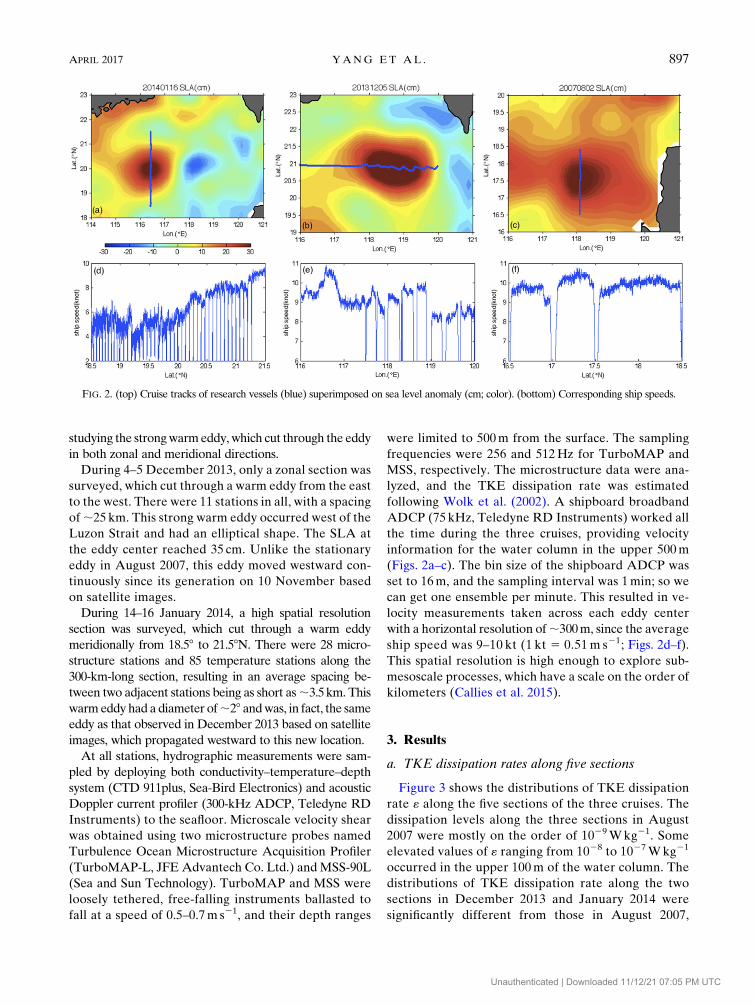
During 4–5 December 2013, only a zonal section was

surveyed, which cut through a warm eddy from the east

to the west. There were 11 stations in all, with a spacing

of;25 km. This strong warm eddy occurred west of the

Luzon Strait and had an elliptical shape. The SLA at

the eddy center reached 35 cm. Unlike the stationary

eddy in August 2007, this eddy moved westward con-

tinuously since its generation on 10 November based

on satellite images.

During 14–16 January 2014, a high spatial resolution

section was surveyed, which cut through a warm eddy

meridionally from 18.58 to 21.58N. There were 28 micro-

structure stations and 85 temperature stations along the

300-km-long section, resulting in an average spacing be-

tween two adjacent stations being as short as;3.5km. This

warmeddy had a diameter of;28 andwas, in fact, the same

eddy as that observed in December 2013 based on satellite

images, which propagated westward to this new location.

At all stations, hydrographic measurements were sam-

pled by deploying both conductivity–temperature–depth

system (CTD 911plus, Sea-Bird Electronics) and acoustic

Doppler current profiler (300-kHz ADCP, Teledyne RD

Instruments) to the seafloor. Microscale velocity shear

was obtained using two microstructure probes named

Turbulence Ocean Microstructure Acquisition Profiler

(TurboMAP-L, JFE Advantech Co. Ltd.) and MSS-90L

(Sea and Sun Technology). TurboMAP and MSS were

loosely tethered, free-falling instruments ballasted to

fall at a speed of 0.5–0.7m s21, and their depth ranges

were limited to 500m from the surface. The sampling

frequencies were 256 and 512Hz for TurboMAP and

MSS, respectively. The microstructure data were ana-

lyzed, and the TKE dissipation rate was estimated

following Wolk et al. (2002). A shipboard broadband

ADCP (75 kHz, Teledyne RD Instruments) worked all

the time during the three cruises, providing velocity

information for the water column in the upper 500m

(Figs. 2a–c). The bin size of the shipboard ADCP was

set to 16m, and the sampling interval was 1min; so we

can get one ensemble per minute. This resulted in ve-

locity measurements taken across each eddy center

with a horizontal resolution of;300m, since the average

ship speed was 9–10 kt (1 kt 5 0.51m s21; Figs. 2d–f).

This spatial resolution is high enough to explore sub-

mesoscale processes, which have a scale on the order of

kilometers (Callies et al. 2015).

3. Results

a. TKE dissipation rates along five sections

Figure 3 shows the distributions of TKE dissipation

rate « along the five sections of the three cruises. The

dissipation levels along the three sections in August

2007 were mostly on the order of 1029Wkg21. Some

elevated values of « ranging from 1028 to 1027Wkg21

occurred in the upper 100m of the water column. The

distributions of TKE dissipation rate along the two

sections in December 2013 and January 2014 were

significantly different from those in August 2007,

FIG. 2. (top) Cruise tracks of research vessels (blue) superimposed on sea level anomaly (cm; color). (bottom) Corresponding ship speeds.

APRIL 2017 YANG ET AL . 897

Unauthenticated | Downloaded 11/12/21 07:05 PM UTC

with higher dissipation values between 1027 and

1026W kg21, muchmore pronounced in the upper 200m.

The difference could come from two factors. The first

factor is latitudinal difference. The two sections sur-

veyed in December 2013 and January 2014 were lo-

cated north of 188N, and the three sections surveyed in

August 2007 were south of 188N. Turbulence in the

SCS generally becomes weaker from the north to the

south (Liu and Lozovatsky 2012; Yang et al. 2016),

since its energy source mainly comes from internal

tides, which are generated in the Luzon Strait and

propagate southwestward into the central SCS. The

energy flux of internal tides becomes weaker from the

north to the south along the propagating path. For

example, Zhao (2014) pointed out that the M2 internal

tide was hardly detected south of 168N.Our results here

show a consistent spatial pattern, which was about one

order weaker from north of 188N to south of 188N. The

second factor is seasonal variability, caused by seasonal

variations of wind and internal tide. Wind is generally

stronger in winter than in summer in the SCS and so is

internal tide. Liu et al. (2015) observed enhanced in-

ternal tides in winter in the northern SCS. Although

the observation periods in this study were short, we

FIG. 3. Spatial distributions of TKE dissipation rate (Wkg21; logarithmic scale) along the sections surveyed in

(a)–(c) August 2007 (18.58, 18.08, and 17.58N), (d) December 2013, and (e) January 2014.

898 JOURNAL OF PHYS ICAL OCEANOGRAPHY VOLUME 47

Unauthenticated | Downloaded 11/12/21 07:05 PM UTC

could infer that the turbulence in winter was more

active than that in summer in the SCS (Sun et al. 2016).

Based on the Osborn (1980) model, eddy diffusivity is

calculated by taking mixing efficiency as a constant.

Here, we use 0.2, as in some studies of frontal regions

(e.g., St. Laurent et al. 2012; Sheen et al. 2013). The

associated diffusivity values with these TKE dissipa-

tion rates ranged from 1024 to 1023m2 s21, consistent

with previous studies (e.g., Liu and Lozovatsky 2012;

Yang et al. 2014b).

b. TKE dissipation rate in the mixed layer

Here, we focus on spatial variation of TKE dissipa-

tion rate; specifically, we compare the rate in the eddy

center with that in the eddy periphery. Based on the

velocity data measured by the shipboard ADCP, we

defined the center and periphery for each eddy first. We

examined the velocity component perpendicular to the

section. For example, we examined the u component

for the meridional section in January 2014 and found

the velocity across the eddy increased from zero at

20.008N to maximum values of 21.0m s21 at 19.508Nand 0.9m s21 at 20.458N (Fig. 4a). For the eddy in De-

cember 2013, the y component of velocity increased

from zero at 118.508E to maximum values of21.5m s21

at 117.88E and 21.4m s21 at 119.308E (Fig. 4b). Al-

though the velocity across the eddy in August 2007 was

weak, its variation trend was the same as those in De-

cember 2013 and January 2014 (Fig. 4c). We defined

the eddy center as the area where the velocity increased

outward until it reached its maximum. So, the enclosed

SLA contour passing through the two locations with

maximum velocities was the outer edge of the eddy

center. We defined the range from the maximum ve-

locity to the outermost enclosed SLA contour as the

eddy periphery. These definitions are consistent with

the features in the cross-track gradient of potential

density based on high spatial resolution sampling (Fig. 4a).

Sharp potential density gradient corresponded to the

locations of velocity maxima well. This density gra-

dient was not examined for the eddies surveyed in

December 2013 and August 2007 because we did not

have as high-resolution measurements as those in

January 2014.

The center and periphery for the three eddies are

shown in Figs. 4d–f, respectively. With this definition,

there were 15 profiles in the eddy periphery, and 17

profiles in the eddy center. For each eddy, the dissi-

pation profiles were averaged over the eddy periphery

and the eddy center, respectively (Fig. 5). The results

show that the mean values of TKE dissipation rate

in the upper layer were obviously elevated in the

eddy periphery for all three eddies, being 5–7 times

larger than those in the eddy center. Thicknesses of

these layers with high TKE dissipation rate ranged

from 70 to 80m for these three eddies, which were

consistent with the mixed layer depths based on the

vertical profiles of temperature and potential density

(Fig. 6). Here, we defined the bottom of the surface

mixed layer using the difference from the surface den-

sity greater than 0.125 kgm23 (e.g., Rimac et al. 2016).

We conclude that the turbulent mixing in the mixed

layer was elevated in the periphery of each warm me-

soscale eddy surveyed.

FIG. 4. (a)–(c) Horizontal velocity component along the cruise track shown in Fig. 2 and (d)–(f) the defined eddy center and periphery.

Sea level anomaly (cm) is shown in color in the bottom panels, from left to right, the dates are January 2014, December 2013, and August

2007. The light blue curve in (a) is the horizontal gradient of potential density along the cruise track.

APRIL 2017 YANG ET AL . 899

Unauthenticated | Downloaded 11/12/21 07:05 PM UTC

4. Discussion and summary

a. Wind and buoyancy flux

It is important to understand what kind of dynamic

process in the mixed layer could drive such elevated

turbulent mixing in the periphery of these mesoscale

eddies. The two most obvious candidates are wind and

buoyancy flux, which are the basic driving force of

mixing in the mixed layer. Hence, we examined obser-

vation dates and times and wind and buoyancy flux for

dissipation profiles in the eddy center and periphery,

respectively (Table 1). Visually, nearly all profiles in the

eddy periphery were collected in the daytime, except for

one profile sampled at an early morning [0559 local time

(LT) on 15 January 2014]. In contrast, half of the profiles

FIG. 5. Mean dissipation profiles in the eddy periphery (black)

and in the eddy center (red) for the three warm eddies in

(a) August 2007, (b) December 2013, and (c) January 2014.

FIG. 6. Selected (a) temperature and (b) potential density pro-

files in the periphery of the three eddies observed in August 2007,

December 2013, and January 2014. The various colors indicate

profiles collected at different dates/times.

900 JOURNAL OF PHYS ICAL OCEANOGRAPHY VOLUME 47

Unauthenticated | Downloaded 11/12/21 07:05 PM UTC

in the eddy center were collected at night. The wind

during each observation period varied only slightly. To

quantify the contributions of wind and buoyancy flux to

the TKE dissipation rate in the mixed layer, we esti-

mated wind energy flux E10 and buoyancy flux J0b. Here,

E10 is given by

E105 r

aC

DU3

10 ,

where ra is air density (1.2 kgm23), drag coefficient

CD5 1.143 1023 (Large and Pond 1981), andU10 is the

wind speed at 10-m height above the sea surface. The

procedure for calculating J0b can be found in Shay and

Gregg (1986), which requires a total of 15 parameters.

Among them, seven parameters were constants, five

parameters were taken from the shipboard meteoro-

logical measurements, and the rest (three parameters)

were obtained from the daily ERA-Interim dataset, at a

time interval of 6 h. We assumed a fraction of 1%, as in

Oakey and Elliott (1982), for the wind energy flux that

entered the mixed layer to support turbulent dissipation.

Based on this assumption, the mean dissipation level

caused by bothwind and buoyancy flux during the survey

periods of the profiles shown in Table 1 was about

1.4 3 1027Wkg21. This value was comparable to the

mean TKE dissipation rate of these three eddies in the

eddy center of 2.13 1027Wkg21, but only about 16%of

the mean dissipation value of 8.7 3 1027Wkg21 in the

eddy periphery. This large difference indicates that other

process contributed to the active turbulence in the pe-

riphery of the three mesoscale eddies.

b. Submesoscale motion

Both numerical simulations and satellite observations

suggest that submesoscale motions are frequently cre-

ated from mesoscale eddies and can be detected clearly

in the eddy periphery (e.g., Capet et al. 2008a; Gaultier

et al. 2014). Submesoscale motion provides a dynamic

conduit for energy transfer toward microscale dissi-

pation and diapycnal mixing (McWilliams 2016). We

TABLE 1. Information on the profiles collected in the center and periphery for three eddies in January 2014, December 2013, and

August 2007.

Station Date Time (LT) Wind (m s21) Buoyancy flux (3 1027Wkg21)

January 2014 Center 01 15 Jan 2014 1817 9.1 2.3

Center 02 15 Jan 2014 2111 9.8 1.5

Center 03 16 Jan 2014 1211 8.8 0.0

Center 04 16 Jan 2014 0310 9.8 1.7

Center 05 16 Jan 2014 0430 9.4 1.9

Center 06 16 Jan 2014 0708 9.3 1.6

Center 07 16 Jan 2014 0918 9.0 1.1

Periphery 01 15 Jan 2014 0559 9.5 0.9

Periphery 02 15 Jan 2014 0843 10.5 0.7

Periphery 03 15 Jan 2014 1239 10.1 21.1

Periphery 04 15 Jan 2014 1527 9.4 20.9

Periphery 05 16 Jan 2014 1130 8.8 0.0

Periphery 06 16 Jan 2014 1331 8.0 20.7

Periphery 07 16 Jan 2014 1524 7.9 20.6

Periphery 08 16 Jan 2014 1719 7.9 20.1

December 2013 Center 01 4 Dec 2013 1615 7.3 20.7

Center 02 4 Dec 2013 2021 7.6 1.1

Center 03 5 Dec 2013 0252 7.6 1.0

Center 04 5 Dec 2013 0746 7.0 0.7

Periphery 01 4 Dec 2013 1001 6.8 21.4

Periphery 02 5 Dec 2013 1313 6.3 20.7

Periphery 03 5 Dec 2013 1456 6.4 20.8

Periphery 04 5 Dec 2013 1647 6.5 1.3

August 2007 Center 01 3 Aug 2007 0718 6.3 0.0

Center 02 3 Aug 2007 1602 6.3 20.7

Center 03 3 Aug 2007 2036 6.1 0.2

Center 04 5 Aug 2007 1122 6.5 0.0

Center 05 5 Aug 2007 1521 5.4 0.8

Center 06 7 Aug 2007 0120 6.1 0.9

Periphery 01 3 Aug 2007 1024 6.4 20.8

Periphery 02 7 Aug 2007 0715 5.5 1.0

Periphery 03 5 Aug 2007 0754 6.5 1.4

APRIL 2017 YANG ET AL . 901

Unauthenticated | Downloaded 11/12/21 07:05 PM UTC

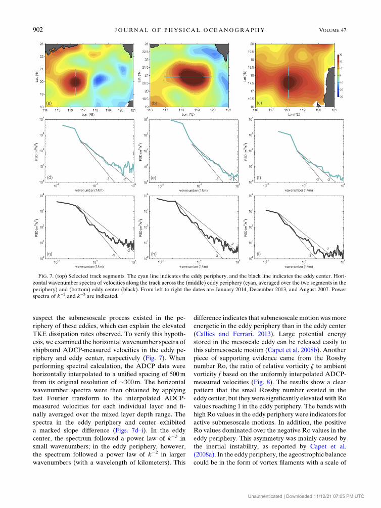
suspect the submesoscale process existed in the pe-

riphery of these eddies, which can explain the elevated

TKE dissipation rates observed. To verify this hypoth-

esis, we examined the horizontal wavenumber spectra of

shipboard ADCP-measured velocities in the eddy pe-

riphery and eddy center, respectively (Fig. 7). When

performing spectral calculation, the ADCP data were

horizontally interpolated to a unified spacing of 500m

from its original resolution of ;300m. The horizontal

wavenumber spectra were then obtained by applying

fast Fourier transform to the interpolated ADCP-

measured velocities for each individual layer and fi-

nally averaged over the mixed layer depth range. The

spectra in the eddy periphery and center exhibited

a marked slope difference (Figs. 7d–i). In the eddy

center, the spectrum followed a power law of k23 in

small wavenumbers; in the eddy periphery, however,

the spectrum followed a power law of k22 in larger

wavenumbers (with a wavelength of kilometers). This

difference indicates that submesoscale motion was more

energetic in the eddy periphery than in the eddy center

(Callies and Ferrari. 2013). Large potential energy

stored in the mesoscale eddy can be released easily to

this submesoscale motion (Capet et al. 2008b). Another

piece of supporting evidence came from the Rossby

number Ro, the ratio of relative vorticity z to ambient

vorticity f based on the uniformly interpolated ADCP-

measured velocities (Fig. 8). The results show a clear

pattern that the small Rossby number existed in the

eddy center, but they were significantly elevatedwithRo

values reaching 1 in the eddy periphery. The bands with

high Ro values in the eddy periphery were indicators for

active submesoscale motions. In addition, the positive

Ro values dominated over the negative Ro values in the

eddy periphery. This asymmetry was mainly caused by

the inertial instability, as reported by Capet et al.

(2008a). In the eddy periphery, the ageostrophic balance

could be in the form of vortex filaments with a scale of

FIG. 7. (top) Selected track segments. The cyan line indicates the eddy periphery, and the black line indicates the eddy center. Hori-

zontal wavenumber spectra of velocities along the track across the (middle) eddy periphery (cyan, averaged over the two segments in the

periphery) and (bottom) eddy center (black). From left to right the dates are January 2014, December 2013, and August 2007. Power

spectra of k22 and k23 are indicated.

902 JOURNAL OF PHYS ICAL OCEANOGRAPHY VOLUME 47

Unauthenticated | Downloaded 11/12/21 07:05 PM UTC

kilometers, which could be detected from remote sens-

ing images. A composite sea surface temperature map

over 3–5 December 2013 from the MODIS level-2

product revealed this kind of filaments around the

eddy periphery (Fig. 9).

We also investigated the kinetic energy distribution of

both mesoscale and submesoscale motions along the

transection using our cruise data. The mesoscale and

submesoscale velocities were obtained by applying

20-km low-pass and high-pass filters to the shipboard

ADCP-measured velocities, respectively. The kinetic

energy was defined as KE5 (1/2)Ð 02MLD

r(u2 1 y2) dz,

where MLD is mixed layer depth. The results suggest

that submesoscale motion was significant in the eddy

periphery but relatively weak in the eddy center. The

kinetic energy of submesoscale motion accounted for up

to 74% in the eddy periphery and was only about one-

quarter in the eddy center in January 2014 (Fig. 10).

Although the high-pass-filtered data may include the

FIG. 8. Variation of Rossby number with depth along the cruise track. The dates are

(a) January 2014, (b) December 2013, and (c) August 2007. The dashed lines in each panel

separate the eddy center and the periphery.

FIG. 9. Map of composite sea surface temperature with a hor-

izontal resolution of 1 km. The data are from the MODIS level-2

product and are averaged between 3 and 5 December 2013.

Filaments around the eddy periphery are indicated by two

black arrows.

APRIL 2017 YANG ET AL . 903

Unauthenticated | Downloaded 11/12/21 07:05 PM UTC

information of internal waves and tides, the energy

variation at the order of kilometers caused by these

waves and tides is likely not significant. Similar results

were obtained for the other two eddies. For the eddy

observed in January 2014, the submesoscale motion was

greatly energized in the northern part of the eddy pe-

riphery. This was likely related to the presence of

Dongsha Island there, since the island favors the gen-

eration of submesoscale motion (Zheng et al. 2008).

To identify the direction of energy cascade, we esti-

mated the spectral flux of kinetic energy P, which is

defined as the integral of the local horizontal advective

term in the kinetic energy equation from wavenumber k

to the largest wavenumber ks, corresponding to the grid

size:

P(k)5

ðksk

2Re[uh* � (u

h� c=

huh)](k) dk ,

where uh 5 (u, y) denotes the horizontal velocity vector

measured from the shipboard ADCP, and =h is the

horizontal gradient operator. The structure � represents

FIG. 10. Distributions of kinetic energy of submesoscale and mesoscale motions along the

section in (a) January 2014, (b) December 2013, and (c) August 2007. Kinetic energy is nor-

malized by its maximum value. The dashed lines in each panel separate the eddy center and the

periphery, and the percentage of kinetic energy in each area is also shown.

904 JOURNAL OF PHYS ICAL OCEANOGRAPHY VOLUME 47

Unauthenticated | Downloaded 11/12/21 07:05 PM UTC

the horizontal spectral transform, and ( )* stands for

complex conjugate, with Re( ) indicating the real

part. Computationally, [uh* � (uh � c=huh)] is estimated as

fft(u)*fft(udu/dx1 ydu/dy)1 fft(y)*fft(udy/dx1 ydy/dy),

where fft represents fast fourier transform. For a

meridional section observed in January 2014

or August 2007, [uh* � (uh � c=huh)] is simplified as

fft(u)*fft(ydu/dy)1 fft(y)*fft(ydy/dy). For a zonal sec-

tion observed in December 2013, [uh* � (uh � c=huh)] is

simplified as fft(u)*fft(udu/dx)1 fft(y)*fft(udy/dx).

The spectral flux was calculated individually for each

layer within the mixed layer, and depth-averaged flux

was used to examine the direction of flux transport.

From the definition of spectral flux of kinetic energy,

for a given wavenumber a positive (negative) flux value

indicates a forward (inverse) kinetic energy cascade.

The spectral fluxes of kinetic energy in the eddy center

and periphery for these three eddies are shown in

Fig. 11. The positive values around larger wavenumbers

(at wavelength of kilometers) occurred in the eddy

periphery, indicating a forward energy cascade toward

smaller scales. This suggests that submesoscale motions

in the eddy periphery could be a key factor leading to

the enhanced mixing. In contrast, the energy flux in the

eddy center was transferred backward toward large

scales. However, submesoscale motion cannot directly

provide energy for turbulent mixing because its char-

acteristic length is several orders larger than that for

turbulent dissipation to occur. Submesoscale motion

acts as a bridge, which decreases the scale gap between

mesoscale and microscale processes, and expedites the

occurrence of turbulent mixing.

c. Summary

To summarize, direct microstructure observations

across three warm mesoscale eddies were obtained in

the northern SCS during field experiments, along with

finestructure measurements. An important finding is

that the turbulent mixing in the mixed layer was con-

siderably elevated in the periphery of the three eddies,

where the mixing level was 5–7 times larger than that

in the eddy center. To explore the mechanism behind

the elevated mixing, we carried out analyses of the

horizontal wavenumber spectrum and spectral fluxes

of kinetic energy. The spectral slope showed a power

law of k22 in the eddy periphery and of k23 in the

center, which was consistent with the results that the

kinetic energy of submesoscale motion in the warm

eddy periphery was more greatly energized than that

in the eddy center. Spectral fluxes of kinetic energy

also revealed a forward energy cascade toward smaller

scales at wavelength of kilometers in the eddy pe-

riphery. These results illustrate a route for energy

cascading from balanced mesoscale dynamics to un-

balanced submesoscale behavior, which eventually

furnishes turbulent mixing. However, the eddies stud-

ied in this study were all warm ones. Generation of

submesoscale motion depends on mixed layer depth.

Warm (cold) eddies can deepen (shallow) the mixed

layer depth, which is beneficial (detrimental) for de-

veloping submesoscale motion (Callies et al. 2015).

Therefore, the submesoscale process is more likely to

FIG. 11. Spectral fluxes of kinetic energy in the eddy periphery

(cyan) and eddy center (black) for the three eddies observed in

(a) January 2014, (b) December 2013, and (c) August 2007.

APRIL 2017 YANG ET AL . 905

Unauthenticated | Downloaded 11/12/21 07:05 PM UTC

be generated when encountering a warm eddy than a

cold eddy. As a result, high-level mixing is expected to

occur in the periphery of a warm eddy. In the coming

days, systematic observations involving multiscale

processes are planned to examine the impacts of warm

and cold eddies on turbulent mixing in detail and to

reveal their associated energy cascade routes.

Acknowledgments. This work is jointly supported

by the Natural Science Foundation of China (Grant

41576009), the National Key Basic Research Program

of China (Grant 2014CB745003), State Key Laboratory

of Tropical Oceanography, South China Sea Institute

of Oceanology, Chinese Academy of Science (Project

LTO1601), the NSFC-Shandong Joint Fund for Ma-

rine Science Research Centers (Grant U1406401), the

Foundation for Innovative Research Groups of the

National Natural Science Foundation of China (Grant

41521091), Global Change and Air-Sea Interaction Project

(Grants GASI-IPOVAI-01-03, GASI-03-01-01-03, and

GASI-IPOVAI-01-02), and the National High Tech-

nology Research and Development Program of China

(Grants 2013AA09A501 and 2013AA09A502). The

altimeter products are available from AVISO (www.

aviso.oceanobs.com/), the ERAdata are available through

the ECMWF (http://apps.ecmwf.int/datasets/data/interim-

full-daily/levtype5sfc/), and the MODIS products are

available through the GSFC (https://modis.gsfc.nasa.gov/

data/).

REFERENCES

Buijsman, M., S. Legg, and J. Klymak, 2012: Double-ridge in-

ternal tide interference and its effect on dissipation in

Luzon Strait. J. Phys. Oceanogr., 42, 1337–1356, doi:10.1175/

JPO-D-11-0210.1.

Callies, J., and R. Ferrari, 2013: Interpreting energy and tracer

spectra of upper-ocean turbulence in the submesoscale range

(1–200 km). J. Phys. Oceanogr., 43, 2456–2474, doi:10.1175/

JPO-D-13-063.1.

——, ——, J. M. Klymak, and J. Gula, 2015: Seasonality in sub-

mesoscale turbulence. Nat. Commun., 6, 6862, doi:10.1038/

ncomms7862.

Capet, X., J. C. McWilliams, M. J. Molemaker, and A. F.

Shchepetkin, 2008a: Mesoscale to submesoscale transition in

the California Current System. Part I: Flow structure, eddy

flux, and observational tests. J. Phys. Oceanogr., 38, 29–43,

doi:10.1175/2007JPO3671.1.

——, ——, ——, and ——, 2008b: Mesoscale to submesoscale

transition in the California Current System. Part III: Energy

balance and flux. J. Phys. Oceanogr., 38, 2256–2269, doi:10.1175/

2008JPO3810.1.

Gaultier, L., B. Djath, J. Verron, J. M. Brankart, P. Brasseur, and

A. Melet, 2014: Inversion of submesoscale patterns from a

high-resolution Solomon Sea model: Feasibility assessment.

J. Geophys. Res. Oceans, 119, 4520–4541, doi:10.1002/

2013JC009660.

Jan, S., C.-S. Chern, J. Wang, and S.-Y. Chao, 2007: Generation of

diurnal K1 internal tide in the Luzon Strait and its influence on

surface tide in the South China Sea. J. Geophys. Res., 112,

C06019, doi:10.1029/2006JC004003.

——, R.-C. Lien, and C.-H. Ting, 2008: Numerical study of

baroclinic tides in Luzon Strait. J. Oceanogr., 64, 789–802,

doi:10.1007/s10872-008-0066-5.

Klymak, J., R. Pinkel, C.-T. Liu, A. Liu, and L. David, 2006: Pro-

totypical solitons in the South China Sea.Geophys. Res. Lett.,

33, L11607, doi:10.1029/2006GL025932.

Large, W., and S. Pond, 1981: Open ocean momentum flux

measurements in moderate to strong winds. J. Phys. Oce-

anogr., 11, 324–336, doi:10.1175/1520-0485(1981)011,0324:

OOMFMI.2.0.CO;2.

Lien, R.-C., F. Henyey, B.Ma, andY.Yang, 2014: Large-amplitude

internal solitary waves observed in the northern South China

Sea: Properties and energetics. J. Phys. Oceanogr., 44, 1095–

1115, doi:10.1175/JPO-D-13-088.1.

Liu, J., Y. He, D.Wang, T. Liu, and S. Cai, 2015: Observed enhanced

internal tides in winter near the Luzon Strait. J. Geophys. Res.

Oceans, 120, 6637–6652, doi:10.1002/2015JC011131.

Liu, Z., and I. Lozovatsky, 2012: Upper pycnocline turbulence in

the northern South China Sea. Chin. Sci. Bull., 57, 2302–2306,

doi:10.1007/s11434-012-5137-8.

McWilliams, J. C., 2016: Submesoscale currents in the ocean. Proc.

Roy. Soc., A472, 20160117, doi:10.1098/rspa.2016.0117.Niwa, Y., and T. Hibiya, 2004: Three-dimensional numerical sim-

ulation of M2 internal tides in the East China Sea. J. Geophys.

Res., 109, C04027, doi:10.1029/2003JC001923.

Oakey, N. S., and J. A. Elliott, 1982: Dissipation within the surface

mixed layer. J. Phys. Oceanogr., 12, 171–185, doi:10.1175/

1520-0485(1982)012,0171:DWTSML.2.0.CO;2.

Osborn, T. R., 1980: Estimates of the local rate of vertical diffusion

from dissipation measurements. J. Phys. Oceanogr., 10, 83–89,

doi:10.1175/1520-0485(1980)010,0083:EOTLRO.2.0.CO;2.

Rimac, A., J. Storch, and C. Eden, 2016: The total energy flux

leaving the ocean’s mixed layer. J. Phys. Oceanogr., 46, 1885–

1900, doi:10.1175/JPO-D-15-0115.1.

Shay, T., and M. Gregg, 1986: Convectively driven turbulent mix-

ing in the upper ocean. J. Phys. Oceanogr., 16, 1777–1798,

doi:10.1175/1520-0485(1986)016,1777:CDTMIT.2.0.CO;2.

Sheen, K. L., and Coauthors, 2013: Rates and mechanisms of tur-

bulent dissipation and mixing in the Southern Ocean: Results

from the Diapycnal and Isopycnal Mixing Experiment in the

Southern Ocean (DIMES). J. Geophys. Res. Oceans, 118,

2774–2792, doi:10.1002/jgrc.20217.

Laurent, L., H. Simmons, T. Tang, and Y. Wang, 2011: Turbulent

properties of internal waves in the South China Sea. Ocean-

ography, 24, 78–87, doi:10.5670/oceanog.2011.96.——,A. NaveiraGarabato, J. Ledwell, A. Thurnherr, J. Toole, and

A. Watson, 2012: Turbulence and diapycnal mixing in Drake

Passage. J. Phys. Oceanogr., 42, 2143–2152, doi:10.1175/

JPO-D-12-027.1.

Sun, H., Q. Yang, W. Zhao, X. Liang, and J. Tian, 2016: Temporal

variability of diapycnal mixing in the northern South China

Sea. J. Geophys. Res. Oceans, 121, 8840–8848, doi:10.1002/

2016JC012044.

Tian, J., Q. Yang, and W. Zhao, 2009: Enhanced diapycnal mixing

in the South China Sea. J. Phys. Oceanogr., 39, 3191–3203,

doi:10.1175/2009JPO3899.1.

Wang, G., D. Chen, and J. Su, 2008: Winter eddy genesis in the

eastern South China Sea due to orographic wind jets. J. Phys.

Oceanogr., 38, 726–732, doi:10.1175/2007JPO3868.1.

906 JOURNAL OF PHYS ICAL OCEANOGRAPHY VOLUME 47

Unauthenticated | Downloaded 11/12/21 07:05 PM UTC

Wolk, F., H. Yamazaki, L. Seuront, and R. G. Lueck, 2002: A new

free-fall profiler for measuring biophysical microstructure.

J. Atmos. Oceanic Technol., 19, 780–793, doi:10.1175/

1520-0426(2002)019,0780:ANFFPF.2.0.CO;2.

Xu, J., J. Xie, Z. Chen, S. Cai, and X. Long, 2012: Enhanced

mixing induced by internal solitary waves in the South

China Sea. Cont. Shelf Res., 49, 34–43, doi:10.1016/

j.csr.2012.09.010.

Yang, Q., L. Zhou, J. Tian, and W. Zhao, 2014a: The roles of

Kuroshio intrusion and mesoscale eddy in upper mixing in the

northern South China Sea. J. Coastal Res., 30, 192–198,

doi:10.2112/JCOASTRES-D-13-00012.1.

——, J. Tian, W. Zhao, X. Liang, and L. Zhou, 2014b: Obser-

vations of turbulence on the shelf and slope of northern

South China Sea. Deep-Sea Res. I, 87, 43–52, doi:10.1016/j.dsr.2014.02.006.

——, W. Zhao, X. Liang, and J. Tian, 2016: Three-dimensional

distribution of turbulent mixing in the South China Sea.

J. Phys.Oceanogr., 46, 769–788, doi:10.1175/JPO-D-14-0220.1.

Zhao, W., C. Zhou, J. Tian, Q. Yang, B. Wang, L. Xie, and T. Qu,

2014: Deep water circulation in the Luzon Strait. J. Geophys.

Res. Oceans, 119, 790–804, doi:10.1002/2013JC009587.

Zhao, Z., 2014: Internal tide radiation from the Luzon Strait.

J. Geophys. Res. Oceans, 119, 5434–5448, doi:10.1002/

2014JC010014.

——, V. Klemas, Q. Zheng, and X.-H. Yan, 2004: Remote sensing

evidence for baroclinic tide origin of internal solitary waves in

the northeastern South China Sea. Geophys. Res. Lett., 31,L06302, doi:10.1029/2003GL019077.

Zheng, Q., H. Lin, J. Meng, X. Hu, Y. T. Song, Y. Zhang, and C. Li,

2008: Sub-mesoscale ocean vortex trains in the Luzon Strait.

J. Geophys. Res., 113, C04032, doi:10.1029/2007JC004362.

APRIL 2017 YANG ET AL . 907

Unauthenticated | Downloaded 11/12/21 07:05 PM UTC