In the ACM SIGGRAPH 2004 conference proceedings

Mesh Editing with Poisson-Based Gradient Field Manipulation

Yizhou Yu† Kun Zhou‡ Dong Xu‡§ Xiaohan Shi ‡§ Hujun Bao§ Baining Guo‡ Heung-Yeung Shum‡

† University of Illinois at Urbana-Champaign ‡ Microsoft Research Asia § Zhejiang University

Abstract

In this paper, we introduce a novel approach to mesh editing withthe Poisson equation as the theoretical foundation. The most dis-tinctive feature of this approach is that it modifies the original meshgeometry implicitly through gradient field manipulation. Our ap-proach can produce desirable and pleasing results for both globaland local editing operations, such as deformation, object merg-ing, and smoothing. With the help from a few novel interactivetools, these operations can be performed conveniently with a smallamount of user interaction. Our technique has three key compo-nents, a basic mesh solver based on the Poisson equation, a gradientfield manipulation scheme using local transforms, and a generalizedboundary condition representation based on local frames. Experi-mental results indicate that our framework can outperform previousrelated mesh editing techniques.

CR Categories: I.3.5 [Computer Graphics]: Computational Ge-ometry and Object Modeling—Boundary representations

Keywords: Poisson Equation, Local Transform Propagation,Mesh Deformation, Object Merging, Mesh Filtering

1 Introduction

Mesh editing has long been an active research area in computergraphics. Most existing techniques, such as deformation, Booleanoperations, detail editing and transfer, manipulate vertex positionsexplicitly. The user needs to be extremely careful to avoid artifactsin the resulting mesh. In this paper, we introduce a new mesh edit-ing technique based on gradient field manipulation which implicitlymodifies vertex positions. This technique is capable of producingdesirable results with a small amount of user interaction.

The theoretical foundation of our technique is the Poisson equa-tion which is able to reconstruct a scalar function from a guidancevector field and a boundary condition. The Poisson equation canalso be viewed as an alternative formulation of a least-squares min-imization. With these appealing characteristics, editing a functioncan be achieved by modifying its gradient field and boundary con-dition, and a succeeding reconstruction using the Poisson equation.The motivation of this approach is twofold. First, the gradient is adifferential property that can be modified locally. Subsequent re-construction from the modified gradient can give rise to a globaleffect which would otherwise require a larger amount of user inter-action. Secondly, artifacts introduced during local editing can be

‡This work was done while Dong Xu and Xiaohan Shi were interns atMicrosoft Research Asia.

Figure 1: An unknown mythical creature. Left: mesh componentsfor merging and deformation (the arm), Right: final editing result.

removed during reconstruction because least-squares minimizationtends to distribute errors uniformly across the function.

Despite the frequent appearance of the Poisson equation in vari-ous computational frameworks [Stam 1999; Perez et al. 2003], ap-plying this equation to mesh editing is nontrivial. The unknown inthe Poisson equation is always a scalar function while a mesh can beconsidered as a vector function that has unique differential proper-ties, such as normals and curvature, with geometric interpretations.How can we apply the Poisson equation to mesh geometry? ThePoisson equation involves gradient fields and a boundary conditionwhich are mathematical concepts. It is not obvious how to modifythese two types of information to achieve desirable mesh editingeffects.

Our key contribution is a mesh processing engine based on gradi-ent field manipulation and boundary condition editing. The engineis equipped with novel techniques designed to overcome the afore-mentioned difficulties. First, we regard the mesh geometry (coordi-nates) as scalar functions defined on a mesh surface and introducethe Poisson equation as a basic mesh solver. Second, we design agradient editing scheme for these scalar functions using local trans-formations. Third, we propose generalized boundary conditions en-forced by propagating local frame changes. These techniques willbe elaborated in Section 3.

Our mesh processing engine has been successfully applied tomesh deformation, merging, as well as anisotropic smoothing.These operations have been integrated into a mesh editing systemwith a few novel interactive tools. Our system exhibits several de-sirable features. Both large-scale and detailed deformation can beachieved conveniently by locally manipulating a curve or vertex onthe mesh. Merging meshes with drastically different open bound-aries have been made easier. The shapes of the merged meshes areglobally adjusted to be more compatible with each other. Details ofthese applications will be introduced in Section 4.

1

In the ACM SIGGRAPH 2004 conference proceedings

2 Background and Related Work

The Poisson Equation. Originally emerging from Isaac New-ton’s law of gravitation [Tohline 1999], the Poisson equation withDirichlet boundary condition is formulated as

∇2f = ∇ · w, f |∂Ω = f∗|∂Ω, (1)

where f is an unknown scalar function, w is a guidance vector field,f∗ provides the desirable values on the boundary ∂Ω, ∇2 = ∂2

∂x2 +∂2

∂y2 + ∂2

∂z2 is the Laplacian operator, ∇ ·w = ∂wx∂x

+∂wy

∂y+ ∂wz

∂z

is the divergence of w = (wx, wy, wz).

Vector Field Decomposition. The Poisson equation is closely re-lated to Helmholtz-Hodge vector field decomposition [Abrahamet al. 1988] which uniquely exists for a smooth 3D vector field wdefined in a region Ω:

w = ∇φ + ∇× υ + h, (2)

where φ is a scalar potential field with ∇× (∇φ) = 0, υ is a vectorpotential field with ∇ · (∇ × υ) = 0, and h is a field that is bothdivergence and curl free. The uniqueness of this decompositionrequires proper boundary conditions. The scalar potential field φfrom this decomposition happens to be the solution of the followingleast-squares minimization

minφ

∫ ∫Ω

‖∇φ − w‖2dA, (3)

whose solution can also be obtained by solving a Poisson equation,∇2φ = ∇ · w.

Discrete Fields and Divergence. A prerequisite of solving thePoisson equation over a triangle mesh is to overcome its irregu-lar connectivity in comparison to a regular image or voxel grid.One recent approach to circumvent this difficulty is to approximatesmooth fields with discrete fields first and then redefine the diver-gence for the discrete fields [Polthier and Preuss 2000; Meyer et al.2002; Tong et al. 2003]. A discrete vector field on a triangle meshis defined to be a piecewise constant vector function whose domainis the set of points on the mesh surface. A constant vector is definedfor each triangle, and this vector is coplanar with the triangle. A dis-crete potential field on a triangle mesh is defined to be a piecewiselinear function, φ(x) =

∑iBi(x)φi, with Bi being the piecewise-

linear basis function valued 1 at vertex vi and 0 at all other vertices,and φi being the value of φ at vi. For a discrete vector field w on amesh, its divergence at vertex vi can be defined to be

(Divw)(vi) =∑

Tk∈N(i)

∇Bik · w|Tk| (4)

where N(i) is the set of triangles sharing the vertex vi, |Tk| is thearea of triangle Tk, and ∇Bik is the gradient vector of Bi withinTk. Note that this divergence is dependent on the geometry and1-ring structures of the underlying mesh.

Mesh deformation and editing. Mesh processing includes alarge variety of operations. We are going to focus on three areasmost relevant to this paper, mesh deformation, object merging andmesh detail editing.

Mesh deformation can be classified as lattice-based free-formdeformation (FFD) [Sederberg and Parry 1986; Coquillart 1990;MacCracken and Joy 1996], curve-based [Barr 1984; Chang andRockwood 1994; Lazarus et al. 1994; Singh and Fiume 1998], orpoint-based [Hsu et al. 1992; Bendels and Klein 2003]. One rep-resentative curve-based method is WIRE [Singh and Fiume 1998]

which directly attaches curves to mesh surfaces to achieve defor-mations. [Milliron et al. 2002] presents a general framework forgeometric warps and deformations. [Llamas et al. 2003; Bendelsand Klein 2003] demonstrate that the use of rotations in additionto translations can achieve certain deformations much more con-veniently. [Pauly et al. 2003] supports multiple shape editing op-erations on point-sampled geometry which is not the focus of thispaper.

Object modeling and deformations can be performed at variousresolutions to achieve both global control and local editing [Kobbeltet al. 1998; Guskov et al. 1999; Kobbelt et al. 2000]. In particu-lar, [Kobbelt et al. 1998] introduces a mesh deformation techniqueby solving a constrained minimization of the thin-plate energy ata desirable coarse resolution. The user specifies deformation con-straints through a handle polygon. Original mesh details are addedback to the resulting smooth mesh to produce a final solution. Thistechnique only gives the user limited control over the mesh shapethrough sparse constraints on the handle polygon. The rest of themesh geometry is uniquely determined by the minimization. Incontrast, the method in this paper can achieve better shape con-trol by specifying guidance vector fields as dense constraints overthe editable mesh region. It does not require a multiresolution meshrepresentation which is only used for acceleration.

Mesh deformation is closely related to shape interpolation andmorphing. [Alexa et al. 2000] introduces a shape interpolationtechnique for simplicial complexes. It considers the interiors ofthe given shapes and minimizes distortion in local volumes. It isnontrivial to generalize this technique to mesh deformation sincetriangle meshes are not simplicial complexes in three-dimensionalspaces. With additional constraints imposed on admissible localtransformations, [Sorkine et al. 2004] proposes such a generaliza-tion using Laplacian coordinates.

Boolean operations are often applied to obtain new models froma set of original ones [Biermann et al. 2001]. Continuity at inter-section curves can be improved by local blending or smoothing.[Museth et al. 2002] applied the level set method to such tasks.The method in [Levy 2003] can also perform merging by extrap-olating parameterizations. In this paper, we perform more generalobject merging without 2D parameterizations by connecting objectsat their open boundaries which may have very different shapes.

There have also been various techniques for mesh detail edit-ing. A signal processing approach was presented in [Taubin 1995].Methods [Taubin 2001; Desbrun et al. 2000; Meyer et al. 2002; Tas-dizen et al. 2002; Bajaj and Xu 2003; Yagou et al. 2003; Fleishmanet al. 2003; Jones et al. 2003] have been developed to remove noisewhile preserving important features by generalizing anisotropic dif-fusion [Perona and Malik 1990] onto meshes. Local details can besmoothed or sharpened by using curvature flows and the level setmethod [Museth et al. 2002].

3 A Framework for Poisson Mesh Editing

Given the definitions of discrete fields and their divergence intro-duced in Section 2, the discrete Poisson equation [Tong et al. 2003]can be expressed as

Div(∇φ) = Divw, (5)

which is actually a sparse linear system,

Af = b, (6)

that can be solved numerically using the conjugate gradient method.We still call (5) the Poisson equation for convenience. Note that theunknown in the discrete Poisson equation is still a scalar potentialfield. It would be straightforward to exploit (5) for surface proper-ties defined on a mesh, such as textures.

2

In the ACM SIGGRAPH 2004 conference proceedings

(a)

V1

x′∇

x∇

V2

V3

(X’1 ,Y’1 ,Z’1)

(b)

XZ

Y

(X’3 ,Y’3 ,Z’3)

(X’2 ,Y’2 ,Z’2)(X3 ,Y3 ,Z3)

(X1 ,Y1 ,Z1)

(X2 ,Y2 ,Z2)T

T

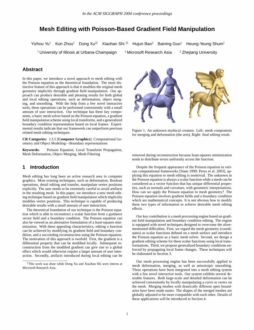
Figure 2: (a) A parameterization mesh, (b) a triangle (red) in theoriginal mesh and its locally transformed version (green). Eachof its coordinates is a scalar function on V1V2V3 in (a). In ad-dition, vertex (Xi, Yi, Zi) corresponds to Vi. ∇x (red) and ∇x′

(green) in (a) are the gradient vectors of the x-component of theoriginal and transformed triangles, respectively. They are coplanarwith V1V2V3.

How can we use the discrete Poisson equation to solve or modifythe mesh geometry itself? Let us describe the fundamentals of thisproblem as well as our solution to boundary condition editing.

3.1 A Basic Poisson Mesh Solver

To apply the discrete Poisson equation to mesh processing, weneed to consider the three coordinates of a target mesh as threescalar fields defined on a parameterization mesh 1. Since trian-gle meshes are piecewise linear models, such scalar fields are ac-tually piecewise linear, and satisfy the definition of discrete poten-tial fields. The target and parameterization meshes should have thesame topology (vertex connectivity), and their vertices should haveone-to-one correspondence.

The purpose of applying the Poisson equation is to solve an un-known target mesh with known topology but unknown geometry(vertex coordinates). To obtain the unknown vertex coordinates, thePoisson equation requires a discrete guidance vector field for eachof the three coordinates. Once a discrete guidance vector field isintroduced over the parameterization mesh, its divergence, definedin (4), at a vertex of the parameterization mesh can be computed.The vector b in (6) is obtained from the the collection of divergencevalues at all vertices. The coefficient matrix A in (6) is independentof the guidance field, and can be obtained using the parameteriza-tion mesh only. The resulting linear system is solved to obtain onespecific coordinate for all vertices simultaneously. This process isrepeated three times to obtain the 3D coordinates of all vertices.This whole process looks like ”mesh cloning”, and the guidancefields encode the desired properties of the target mesh.

In principle, different parameterization meshes give rise to dif-ferent target meshes. Due to the nature of the least-squares mini-mization in (3), the general rule is that guidance vectors associatedwith larger triangles in the parameterization mesh are better approx-imated than those associated with smaller triangles. The areas ofthe triangles serve as the weighting scheme. During mesh editing,the original mesh is given and the goal is to obtain an edited mesh.Therefore, it is most convenient to treat the original mesh as the pa-rameterization mesh and the edited one as the target mesh withoutany 2D parameterizations.

1The concept of a parameterization mesh has previously been used in[Taubin 1995; Karni and Gotsman 2000], however, not in the context ofthe Poisson equation. In addition, their parameterization meshes only havetopology while ours are real 3D meshes.

BC

BC’

F’

F

(a) (b)

(c) (d)

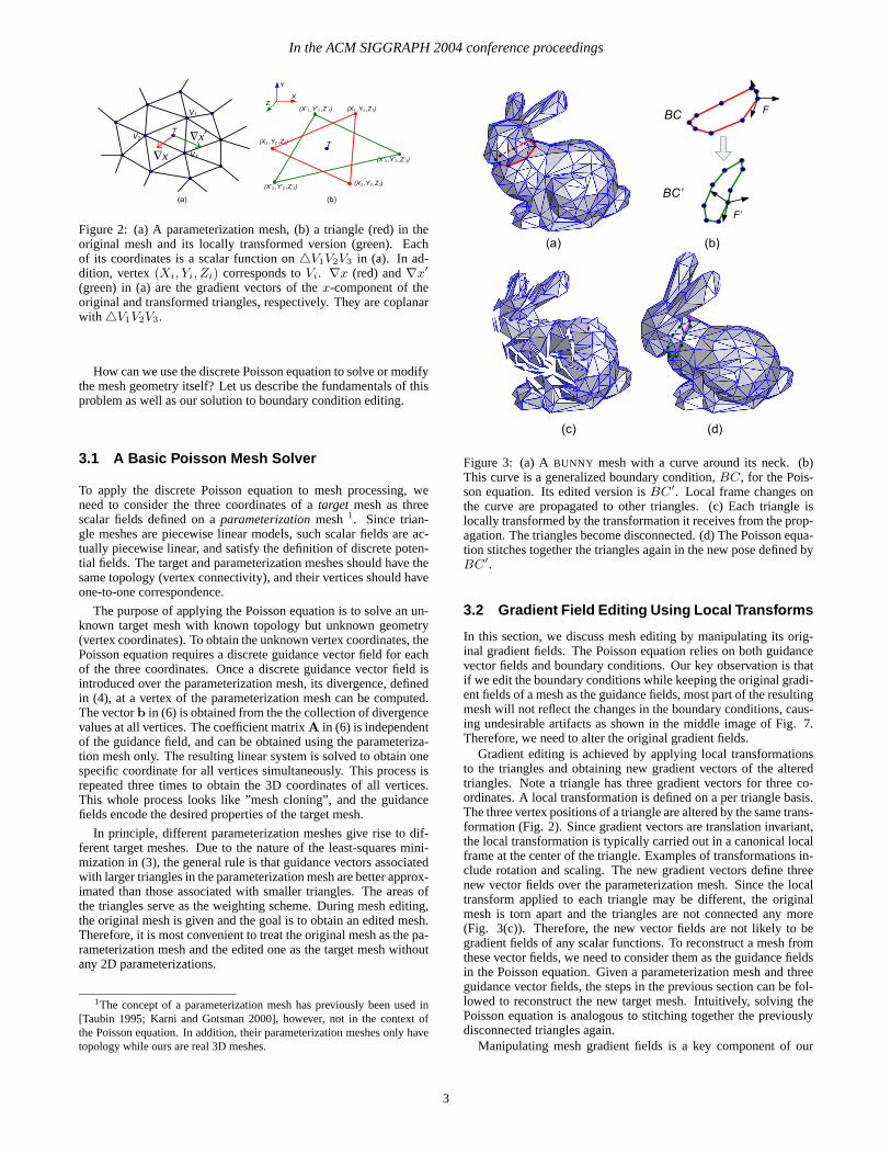
Figure 3: (a) A BUNNY mesh with a curve around its neck. (b)This curve is a generalized boundary condition, BC, for the Pois-son equation. Its edited version is BC′. Local frame changes onthe curve are propagated to other triangles. (c) Each triangle islocally transformed by the transformation it receives from the prop-agation. The triangles become disconnected. (d) The Poisson equa-tion stitches together the triangles again in the new pose defined byBC′.

3.2 Gradient Field Editing Using Local Transforms

In this section, we discuss mesh editing by manipulating its orig-inal gradient fields. The Poisson equation relies on both guidancevector fields and boundary conditions. Our key observation is thatif we edit the boundary conditions while keeping the original gradi-ent fields of a mesh as the guidance fields, most part of the resultingmesh will not reflect the changes in the boundary conditions, caus-ing undesirable artifacts as shown in the middle image of Fig. 7.Therefore, we need to alter the original gradient fields.

Gradient editing is achieved by applying local transformationsto the triangles and obtaining new gradient vectors of the alteredtriangles. Note a triangle has three gradient vectors for three co-ordinates. A local transformation is defined on a per triangle basis.The three vertex positions of a triangle are altered by the same trans-formation (Fig. 2). Since gradient vectors are translation invariant,the local transformation is typically carried out in a canonical localframe at the center of the triangle. Examples of transformations in-clude rotation and scaling. The new gradient vectors define threenew vector fields over the parameterization mesh. Since the localtransform applied to each triangle may be different, the originalmesh is torn apart and the triangles are not connected any more(Fig. 3(c)). Therefore, the new vector fields are not likely to begradient fields of any scalar functions. To reconstruct a mesh fromthese vector fields, we need to consider them as the guidance fieldsin the Poisson equation. Given a parameterization mesh and threeguidance vector fields, the steps in the previous section can be fol-lowed to reconstruct the new target mesh. Intuitively, solving thePoisson equation is analogous to stitching together the previouslydisconnected triangles again.

Manipulating mesh gradient fields is a key component of our

3

In the ACM SIGGRAPH 2004 conference proceedings

mesh editing system. This editing mode will be exploited in thefollowing section as well as Section 4.3. Note that it would betedious to interactively define a local transform for every triangleof a mesh. Automatic schemes to obtain such local transforms willbe discussed wherever gradient manipulation is needed.

3.3 Boundary Condition Editing

We would like to achieve local or global mesh editing by con-veniently manipulating a small number of local features such ascurves or vertices. In this section, we discuss how to satisfy suchediting requests. Details about user interaction will be discussed inSection 4. In terms of the Poisson equation, both a curve or a ver-tex anywhere on a mesh is a boundary condition in the sense thata unique solution to the Poisson equation exists because this equa-tion is translation invariant. There is still something more to meshesthan to scalar functions. Geometrically, a set of neighboring ver-tices on a mesh provides information such as normal orientation,curvature and scale in addition to the vertex positions themselves.Therefore, there is a need to generalize the concept of a boundarycondition for a mesh.

We formally define a generalized boundary condition of a meshas a combination of five components BC = (I, P, F, S, R) whereI is the index set of a set of connected vertices on the mesh, Pis the set of 3D vertex positions, F is a set of local frames whichdefine the local orientations of the vertices, S is the set of scalingfactors associated with the vertices, and R is a strength field. A ver-tex is constrained if it belongs to at least one boundary condition;otherwise, it is a free vertex. As usual, a local frame at a vertex isdefined by three orthogonal unit vectors one of which should be theunit normal. If a vertex belongs to a curve, its local frame shouldbe defined by the normal, the tangent and the binormal of the curve.The scaling factor at a vertex only reflects the scale change beforeand after an editing operation, and can be initialized to one at thebeginning. The strength field defines the influence of the boundarycondition at every free vertex. The influence (strength) is a functionof the minimal distance between the free vertex and the constrainedvertices in the boundary condition. All free vertices receiving anonzero strength define the influence region of the boundary condi-tion.

Once a boundary condition BC = (I, P, F, S, R) needs editing,we create a modified version BC′ = (I, P ′, F ′, S′, R) (Fig. 3(b)).A constrained vertex position vc ∈ P may have a different position,local frame and scale in BC′. The difference between the newand old local frames at vi can be uniquely determined by a singlerotation which is represented as a unit quaternion in practice. Thedifference in scale is represented as a ratio. Thus, each constrainedvertex in BC has its associated quaternion and ratio to representthe local frame and scale changes.

We propagate the local frame and scale changes from the con-strained vertices to all the free vertices in the influence region tocreate a smooth transition. When there is only one single bound-ary condition, BC0 = (I0, P0, F0, S0, R0), and its edited version,BC′

0, we first compute the geodesic distance from each free vertex,denoted by vf , in the original mesh to all the constrained verticesin BC0

2. Suppose vmin is the constrained vertex in BC0 that isclosest to vf . That is, vmin = arg minvc∈P0 dist(vf ,vc). Thesimplest scheme, called the Nearest scheme, directly assigns thequaternion and scale ratio at vmin to vf . In practice, smoother re-sults can be obtained by assigning to vf the weighted average ofthe quaternions and scale ratios at all constrained vertices in BC0.We designed three weighting schemes: Uniform, Linear, and Gaus-sian. In the Uniform scheme, the transforms from all constrained

2This is actually a distance transform that can be computed by the levelset method [Sethian 1999].

(c)(a) (b)

Figure 4: (a) Original model (2040 vertices and 4000 faces), (b)twisting by rotating the top rectangular boundary around the ver-tical axis of the PRISM (running time = 578 ms), (c) bending byrotating the top boundary around a horizontal axis in addition to atranslation (running time = 609 ms).

(c)(b)(a)

Figure 5: (a) Original model (1281 vertices and 2480 faces), (b)-(c)simultaneous normal rotation around their respective tangents usingcosine functions with two different phase angles as their strengthfields. The running time for (b) is 230ms and (c) 240ms.

vertices in BC0 are weighed equally. In the Linear scheme, thetransform from a constrained vertex, vc, in BC0 is weighed bythe inverse of dist(vf ,vc). In the Gaussian scheme, the transformfrom a constrained vertex, vc, in BC0 is weighed by the Gaus-

sian function exp(− (dist(vf ,vc)−dist(vf ,vmin))2

2σ2d

), where σd is a

user-specified parameter to indicate the width of the Gaussian. Inour experiments, the Linear and Gaussian weighting schemes typi-cally produce better results.

When there are multiple boundary conditions, BCi, i =1, ..., m, a free vertex vf receives a quaternion qi from each of theboundary conditions. We define a weight wi for each quaternion qi

using the strength of BCi at vf . The strength of a boundary con-dition in its influence region can be constant, linearly decreasing ora cosine wave function. The final quaternion assigned to vf is a

weighted average,

∑i

wiqi∑i

wi

3. The final scale ratio can be defined

similarly using the geometric mean.We proceed to define a local transform for each triangle in the

mesh. An average quaternion based on the three quaternions at thethree vertices represents the rotation component. The scale ratiorepresents the scaling factor. Both rotation and scaling can be in-tegrated into a single linear transform applied to the triangle as inSection 3.2 to obtain new guidance vectors. The new mesh geom-etry obtained using the solver in Section 3.1 best approximates theorientations and scales imposed by the modified generalized bound-ary conditions (Fig. 3(d)).

3Note that we frequently use (weighted) averages of quaternions.Since quaternions are not commutative, such a weighted average is im-plemented by a sequence of spherical-linear interpolations in a fixedorder. For example, w1q1+w2q2+w3q3

w1+w2+w3is actually interpreted as

w1+w2w1+w2+w3

(w1

w1+w2q1 + w2

w1+w2q2

)+ w3

w1+w2+w3q3.

4

In the ACM SIGGRAPH 2004 conference proceedings

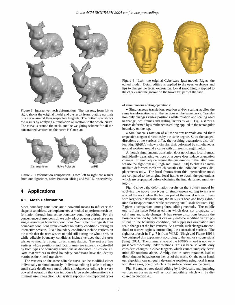
Figure 6: Interactive mesh deformation. The top row, from left toright, shows the original model and the result from rotating normalsof a curve around their respective tangents. The bottom row showsthe results by applying a translation or rotation to the whole curve.The curve is around the neck, and the weighting scheme for all theconstrained vertices on the curve is Gaussian.

WIRENaïve PoissonOur algorithm

Figure 7: Deformation comparison. From left to right are resultsfrom our algorithm, naive Poisson editing and WIRE, respectively.

4 Applications

4.1 Mesh Deformation

Since boundary conditions are a powerful means to influence theshape of an object, we implemented a method to perform mesh de-formation through interactive boundary condition editing. For theconvenience of user control, we only adopt open or closed curves orsingle vertices as boundary conditions. We further distinguish fixedboundary conditions from editable boundary conditions during aninteractive session. Fixed boundary conditions include vertices onthe mesh that the user wishes to hold still during the whole sessionwhile editable boundary conditions include vertices that the userwishes to modify through direct manipulation. The rest are freevertices whose positions and local frames are indirectly controlledby both types of boundary conditions as discussed in Section 3.3.Note that vertices in fixed boundary conditions have the identitymatrix as their local transform.

The vertices on the same editable curve can be modified eitherindividually or simultaneously. Individual editing is able to changesmall scale details on a mesh while simultaneous editing is a verypowerful operation that can introduce large scale deformations viaminimal user interaction. Our system supports two important types

Figure 8: Left: the original Cyberware Igea model; Right: theedited model. Detail editing is applied to the eyes, eyebrows andlips to change the facial expression. Local smoothing is applied tothe cheeks and the groove on the lower left part of the face.

of simultaneous editing operations:• Simultaneous translation, rotation and/or scaling applies the

same transformation to all the vertices on the same curve. Transla-tion only changes vertex positions while rotation and scaling needto change local frames and scaling factors as well. Fig. 4 shows aPRISM deformed by simultaneous editing applied to the rectangularboundary on the top.

• Simultaneous rotation of all the vertex normals around theirrespective tangent directions by the same degree. Since the tangentdirections at the vertices differ, the resulting quaternions also dif-fer. Fig. 5(b)&(c) show a circular disk deformed by simultaneousnormal rotation around a curve with different strength fields.

Although simultaneous translation does not change local frames,individually translating vertices on a curve does induce orientationchanges. To uniquely determine the quaternions in the latter case,we use the algorithm in [Singh and Fiume 1998] to obtain an inter-mediate deformed mesh which satisfies the individual vertex dis-placements only. The local frames from this intermediate meshare compared to the original local frames to obtain the quaternionswhich are propagated before obtaining the final deformed mesh us-ing (6).

Fig. 6 shows the deformation results on the BUNNY model byapplying the above two types of simultaneous editing to a curvearound the neck when the bottom part of the model is fixed. Evenwith large-scale deformations, the BUNNY’s head and body exhibitnice elastic appearances while preserving small-scale features. Fig.7 gives a comparison among three editing methods. The middleone is from naive Poisson editing which does not propagate lo-cal frame and scale changes. It has severe distortions because thePoisson equation by default can only enforce modified vertex po-sitions in the boundary condition, but suppresses orientation andscale changes at the free vertices. As a result, such changes are con-fined to narrow regions surrounding the constrained vertices. Therightmost result in Fig. 7 is from WIRE [Singh and Fiume 1998].We designed this experiment according to the author’s suggestions[Singh 2004]. The original shape of the BUNNY’s head is not well-preserved especially under rotations. This is because WIRE onlyconsiders changes in curve tangents which cannot uniquely deter-mine 3D rotations alone. Ambiguities in curve rotations lead todiscontinuous behaviors on the rest of the mesh. On the other hand,our algorithm can uniquely determine rotations using local frameswith three axes, one of which is the surface normal on the curve.

Fig. 8 demonstrates detail editing by individually manipulatingvertices on curves as well as local smoothing which will be dis-cussed in Section 4.3.

5

In the ACM SIGGRAPH 2004 conference proceedings

(c) (d)

(a) (b)

Figure 9: (a) the boundary on the WING (2000 faces) is projectedalong a user-defined direction to define the boundary on the HORSEmodel ( 100K faces), (b) the result from our projection scheme (run-ning time = 400 ms), (c) Boolean operation, (d) WIRE.

4.1.1 Acceleration for Interactive Deformation

The Poisson equation is a sparse linear system that can be efficientlysolved by the conjugate gradient method. However, according tothe timings shown in Fig. 4 and 5, when the number of vertices inthe mesh becomes large, it is impossible to achieve interactive ratesby solving the equation at the original resolution. Since interactiveperformance is critical for user-guided deformation, we introduce afew acceleration schemes particularly for this task.

If we look at the linear system in (6), matrix A is only dependenton the parameterization mesh and the original target mesh beforeediting while b is also dependent on the current guidance vectorfield. Therefore, A is fixed as long as we do not switch the parame-terization mesh while b changes constantly during interactive meshediting. Thus, we can precompute A−1 using LU decomposition,and only dynamically execute the back substitution step to obtainA−1b at every frame. Our experiments indicate that this schemealone can achieve a three to six fold speedup. Note that LU decom-position is less stable than conjugate gradient, and does not preservethe sparse structure of matrix A. The latter implies that storing theresult of LU decomposition requires more memory and reduces thelargest mesh size a machine can handle. This acceleration schemeis only used during interactive sessions, and the user can requestthe system to produce a final version of the deformed mesh usingconjugate gradient.

The second acceleration scheme exploits multiresolutionmeshes. We build a multiresolution mesh pyramid for large meshesusing the algorithm presented in [Guskov et al. 1999] and onlyperform Poisson mesh editing at the coarsest resolution. At ev-ery frame, the pyramid is collapsed to add high frequency detailsback onto the modified coarsest level to obtain a modified high res-olution mesh for display. The pyramid collapse operation can beperformed very efficiently. Therefore, this scheme is much moreefficient than directly solving the Poisson equation at the high-

Planar Projection

CylinderMapping

Merging

Figure 10: Object merging using mapping. Only the front facinghalf of the DRAGON model (18K faces) is mapped with its openboundary onto a plane which is then mapped onto the CYLINDER(60K faces). The running time is 5 seconds.

est resolution. Because the level of precision tolerance increaseswith the scale of deformation, we use multiresolution accelerationfor large-scale deformations like those shown in Fig. 6 where thefinest BUNNY model for display has 70K faces and its correspond-ing coarsest model only has 2000 faces.

At the coarsest level of the BUNNY model, our LU-based accel-eration took 29 milliseconds on an Intel Xeon 1.5GHz processorfor each editing operation while the non-accelerated version took105 milliseconds. With both acceleration schemes, our system onlytook around 100 milliseconds at the finest level where the non-accelerated version took multiple seconds. The size of the BUNNYmodel approaches the limit we can handle interactively (10fps) onthe machine we use.

In our system, small-scale editing is directly performed on thefinest level, but confined to a small surface region. With most of themesh vertices fixed, editing in a small region can still be performedin real-time as well. The result shown in Fig. 8 was obtained in thefinest level.

4.2 Mesh Merging and Assembly

Merging meshes to assemble a complete object is another impor-tant application of our framework. The partial meshes are mergedat their open (mesh) boundaries which truly serve as Poisson bound-ary conditions this time! Merging two meshes involves the follow-ing steps: i) obtain a mesh boundary on each mesh and the vertexcorrespondence between them; ii) compute or custom design thelocal frames along the two boundaries; iii) obtain an intermediateboundary, including both vertex positions and local frames, by ei-ther interpolating the original two using the vertex correspondenceor simply choosing one of the original two; iv) change the meshconnectivity along the boundaries of both meshes according to theintermediate boundary. iv) compare the local frames at the inter-mediate boundary with the local frames at the original two bound-aries to obtain two sets of quaternions; v) propagate the two sets ofquaternions towards the interior of both meshes, respectively; vi)set up the linear system in (6) for all the vertices from both meshesand solve it to obtain a merged mesh.

6

In the ACM SIGGRAPH 2004 conference proceedings

(c)

(a)

(b)

Figure 11: Object merging by interactively specifying sparse keyvertex correspondences between two boundaries. GARGOYLE has4000 faces, TEAPOT has 2000 faces, and the running time is 890ms.

Figure 12: Two mesh components are merged at their jaggedboundaries.

The vertex correspondence between boundaries is not automat-ically available in our method. We designed the following threeinteractive tools from which the user can choose. The first tool isquite restrictive but only needs little user interaction while the lastone is most powerful but requires a larger amount of interaction.

i) The boundary on the first mesh is projected onto the secondmesh to obtain the second boundary. The user only needs to inter-actively define a projection direction (Fig. 9(a)). Vertex correspon-dence is obtained by extending every vertex on the first boundaryinto a ray whose nearest vertex on the second mesh is then located.Fig. 9(b) shows a model merged using this tool.

ii) A planar parameterization of the boundary curve on the firstmesh is first obtained. Then this 2D boundary is mapped onto thesecond mesh using a mapping scheme, such as the cylindrical map-ping or more general parameterizations. A model merged using thistool is shown in Fig. 10.

iii) The user interactively defines sparse key vertex correspon-dences between the two boundaries and a dense correspondence isobtained through interpolation. Fig. 11 and 12 show two examplesgenerated using this scheme.

Using our method to perform mesh merging has the followingmajor advantages:

• It allows the two mesh boundaries to have very differentshapes, sizes and roughness. For example, in Fig. 9(a), becausethe boundary of the WING is projected along an oblique directiononto the HORSE surface which has undulations, the two boundarieshave different shapes and sizes. The two boundaries in Fig. 12 alsohave different shapes and are jagged.

• The propagation of local frame changes can globally adjustthe two meshes so their shapes become more compatible with eachother. This is demonstrated in Fig. 9(b), 11 and 12. Note that theexample in Fig. 11 would be difficult for parameterization-based

(d)(c)

(a) (b)

Figure 13: Denoising results. (a) Original model (150K vertices),(b) smoothed model of (a) after only one iteration with σf = 4.0and σg = 0.2π. (c) Noisy model (Gaussian noise), (d) smoothedmodel of (c) after three iterations with σf = 3.0 and σg = 0.2π.

merging [Levy 2003] since one of the components has genus greaterthan zero.

A comparison is given in Fig. 9 among three approaches. Fig.9(b) shows our merging result. Fig. 9(c) is from Boolean intersec-tion. To extract a closed intersection curve between the two partialmeshes, we had to lower the WING. As a result, the undulationson the HORSE model hide a large portion of it. The result fromWIRE [Singh and Fiume 1998] is shown in Fig. 9(d) where theWING exhibits the same type of distortions and discontinuities as indeformation.

An example with both deformation and merging is shown in Fig.1. Multiple components are merged and the ARM is deformed be-fore being merged.

Although Poisson mesh deformation and merging are powerfuland flexible, they do not guarantee G1 continuity between con-strained and free vertices. Fortunately, continuity at these placescan be significantly improved by Poisson normal smoothing, whichwill be introduced in the next section.

4.3 Mesh Smoothing and Denoising

The Poisson equation can be applied to perform mesh filtering oper-ations in addition to interactive editing. As an example, we demon-strate a mesh smoothing and denoising algorithm in this section.Our algorithm does feature-preserving mesh smoothing via nor-mals, which have previously been investigated [Taubin 2001; Tas-dizen et al. 2002; Yagou et al. 2003]. In practice, we conduct bilat-eral filtering on the normals instead of the vertex positions [Joneset al. 2003; Fleishman et al. 2003] to preserve sharp features. Us-ing normals to preserve features on a mesh is more intuitive sincenormals typically change abruptly at edges and creases. Actually[Jones et al. 2003] does perform normal smoothing as a prepro-cessing step. The bilateral filters in our method also have two pa-rameters σf and σg . σf controls the spatial weight which is alsoused in [Jones et al. 2003; Fleishman et al. 2003] while σg definesthe amount of normal variation allowed. Once smoothed normalshave been obtained, our algorithm shifts vertex positions using thePoisson equation to reflect the altered normals while [Jones et al.2003] performs a revised bilateral filtering on the vertices. Since

7

In the ACM SIGGRAPH 2004 conference proceedings

Figure 14: Smoothing merging boundary. Left: before smoothing,Right: after smoothing.

the normal of a triangle is a nonlinear function of its vertex posi-tions, reconstructing a mesh from predefined normals is a classicnonlinear optimization problem [Yagou et al. 2003] which is bothexpensive and prone to local suboptimal solutions.

Our engine facilitates a linear method to obtain vertex positionsfrom normals. Consider one triangle with its original normal ni.Suppose we have defined its new normal which is ni

′. To incorpo-rate this change, we define a local rotation matrix from the minimalrotation angle and its associated axis that can transform the originalnormal to the new one. This local rotation matrix serves as the localtransform that should be applied to the original triangle to obtain anew triangle and its new gradient vectors. We perform this stepover all triangles with altered normals to define new guidance fieldsas in Section 3.2. With these new guidance fields, the new vertexpositions of the mesh can be obtained as in Section 3.1.

This smoothing algorithm can be applied to a mesh either onceor with multiple iterations. The solution obtained can be eitherused directly or as the initialization for further nonlinear optimiza-tion. The use of this algorithm includes mesh denoising and meshsmoothing. In the latter case, we replace the bilateral filter with aregular Gaussian filter for normals because we do not wish to pre-serve small features and artifacts. Fig. 13 shows two examples offeature-preserving mesh denoising. Fig. 14 shows the effect of lo-cal smoothing at the merging boundary while Fig. 8 demonstratessmoothing in user-specified local regions.

5 Conclusions

In this paper, we have developed a basic framework along withinteractive tools for mesh editing. The core of the technique is aPoisson mesh solver which has a solid theoretical foundation. Thecomputations and implementations involved are very straightfor-ward. The interactive tools are intuitive, and do not require specialknowledge about the underlying theory. The product is a versa-tile mesh editing system that can be used for high-end applicationswhich require superior results.

In future, we would like to overcome the limitations of the frame-work presented in this paper. The Poisson equation can only guar-antee C0 continuity between constrained and free vertices althoughthe C0 effect is not obvious due to local transform propagation. Itis also possible to improve the performance of our user-guided de-formation by exploiting multi-grid methods.

Acknowledgments: We wish to thank Karan Singh (U.Toronto) for discussion on WIRE, Lin Shi (UIUC) for discussionon the Poisson equation, Yiying Tong (USC) for discussion onvector field decomposition, and the anonymous reviewers for theirvaluable comments. Thanks to Ran Zhou, Bo Zhang and SteveLin (MSRA) for their help in video production. Yizhou Yu wassupported by NSF (CCR-0132970). Hujun Bao was supported byNSFC (No. 60021201 and 60033010) and 973 Program of China(No. 2002CB312104).

ReferencesABRAHAM, R., MARSDEN, J., AND RATIU, T. 1988. Manifolds, Tensor Analysis,

and Applications, vol. 75. Springer. Applied Mathematical Sciences.ALEXA, M., COHEN-OR, D., AND LEVIN, D. 2000. As-rigid-as-possible shape

interpolation. In SIGGRAPH 2000 Conference Proceedings, 157–164.BAJAJ, C., AND XU, G. 2003. Anisotropic diffusion on surfaces and functions on

surfaces. ACM Trans. Graphics 22, 1, 4–32.BARR, A. 1984. Global and local deformations of solid primitives. Computer Graph-

ics(SIGGRAPH’84) 18, 3, 21–30.BENDELS, G., AND KLEIN, R. 2003. Mesh forging: Editing of 3d-meshes using

implicitly defined occluders. In Symposium on Geometry Processing.BIERMANN, H., KRISTJANSSON, D., AND ZORIN, D. 2001. Approximate boolean

operations on free-form solids. In Proceedings of SIGGRAPH, 185–194.CHANG, Y.-K., AND ROCKWOOD, A. 1994. A generalized de casteljau approach to

3d free-form deformation. In Proc. SIGGRAPH’94, 257–260.COQUILLART, S. 1990. Extended free-form deformation: A sculpturing tool for 3d

geometric modeling. Computer Graphics(SIGGRAPH’90) 24, 4, 187–196.DESBRUN, M., MEYER, M., SCHRODER, P., AND BARR, A. 2000. Anisotropic

feature-preserving denoising of height fields and bivariate data. In Proc. GraphicsInterface, 145–152.

FLEISHMAN, S., DRORI, I., AND COHEN-OR, D. 2003. Bilateral mesh denoising.ACM Trans. Graphics 22, 3, 950–953.

GUSKOV, I., SWELDENS, W., AND SCHRODER, P. 1999. Multiresolution signalprocessing for meshes. In Proc. SIGGRAPH’99, 325–334.

HSU, W., HUGHES, J., AND KAUFMAN, H. 1992. Direct manipulation of free-formdeformations. In Proc. SIGGRAPH’92, 177–184.

JONES, T., DURAND, F., AND DESBRUN, M. 2003. Non-iterative, feature-preservingmesh smoothing. ACM Trans. Graphics 22, 3, 943–949.

KARNI, Z., AND GOTSMAN, C. 2000. Spectral compression of mesh geometry. InProc. SIGGRAPH’00, 279–287.

KOBBELT, L., CAMPAGNA, S., VORSATZ, J., AND SEIDEL, H.-P. 1998. Interactivemulti-resolution modeling on arbitrary meshes. In Proc. SIGGRAPH’98, 105–114.

KOBBELT, L., BAREUTHER, T., AND SEIDEL, H.-P. 2000. Multiresolution shapedeformations for meshes with dynamic vertex connectivity. In Proc. Eurograph-ics’2000.

LAZARUS, F., COQUILLART, S., AND JANCENE, P. 1994. Axial deformations: Anintuitive deformation technique. Computer Aided Design 26, 8, 607–613.

LEVY, B. 2003. Dual domain extrapolation. ACM TOG 22, 3, 364–369.LLAMAS, I., KIM, B., GARGUS, J., ROSSIGNAC, J., AND SHAW, C. D. 2003.

Twister: A space-warp operator for the two-handed editing of 3d shapes. ACMTrans. Graphics 22, 3, 663–668.

MACCRACKEN, R., AND JOY, K. 1996. Free-form deformations with lattices ofarbitrary topology. In Proceedings of SIGGRAPH’96, 181–188.

MEYER, M., DESBRUN, M., SCHRODER, P., AND BARR, A. 2002. Discretedifferential-geometry operators for triangulated 2-manifolds. In Proc. VisMath.

MILLIRON, T., JENSEN, R., BARZEL, R., AND FINKELSTEIN, A. 2002. A frame-work for geometric warps and deformations. ACM Trans. Graphics 21, 1, 20–51.

MUSETH, K., BREEN, D., WHITAKER, R., AND BARR, A. 2002. Level set surfaceediting operators. ACM Transactions on Graphics 21, 3, 330–338.

PAULY, M., KEISER, R., KOBBELT, L., AND GROSS, M. 2003. Shape modeling withpoint-sampled geometry. ACM Trans. Graphics 22, 3, 641–650.

PEREZ, P., GANGNET, M., AND BLAKE, A. 2003. Poisson image editing. ACMTrans. on Graphics 22, 313–318.

PERONA, P., AND MALIK, J. 1990. Scale-space and edge detection using anisotropicdiffusion. IEEE Trans. Patt. Anal. Mach. Intell. 12, 7, 629–639.

POLTHIER, K., AND PREUSS, E. 2000. Variational approach to vector field decom-position. In Proc. Eurographics Workshop on Scientific Visualization.

SEDERBERG, T., AND PARRY, S. 1986. Free-form deformation of solid geometricmodels. Computer Graphics(SIGGRAPH’86) 20, 4, 151–160.

SETHIAN, J. 1999. Level Set Methods and Fast Marching Methods. CambridgeUniversity Press.

SINGH, K., AND FIUME, E. 1998. Wires: A geometric deformation technique. InProc. SIGGRAPH’98, 405–414.

SINGH, K., 2004. personal communication.SORKINE, O., COHEN-OR, D., LIPMAN, Y., ALEXA, M., ROSSL, C., AND SEIDEL,

H.-P. 2004. Laplacian surface editing. Tech. rep., March 2004.STAM, J. 1999. Stable fluids. In SIGGRAPH 99 Conference Proceedings, 121–128.TASDIZEN, T., WHITAKER, R., BURCHARD, P., AND OSHER, S. 2002. Geomet-

ric surface smoothing via anisotropic diffusion of normals. In Proceedings IEEEVisualization, 125–132.

TAUBIN, G. 1995. A signal processing approach to fair surface design. In Proc.SIGGRAPH’95, 351–358.

TAUBIN, G. 2001. Linear anisotropic mesh filtering. Tech. rep., IBM Research ReportRC2213.

TOHLINE, J., 1999. Origin of the poisson equation.http://www.phys.lsu.edu/astro/H Book.current/Context/PGE/poisson.origin.text.pdf.

TONG, Y., LOMBEYDA, S., HIRANI, A., AND DESBRUN, M. 2003. Discrete multi-scale vector field decomposition. ACM Trans. Graphics 22, 3, 445–452.

YAGOU, H., OHTAKE, Y., AND BELYAEV, A. 2003. Mesh denoising via iterativealpha-trimming and nonlinear diffusion of normals with automatic thresholding. InProc. Computer Graphics Intl.

8