Insurance Premium Prediction via Gradient

Tree-Boosted Tweedie Compound Poisson

Models

Yi Yang∗, Wei Qian†and Hui Zou‡

April 22, 2016

Abstract

The Tweedie GLM is a widely used method for predicting insurance premiums.

However, the structure of the logarithmic mean is restricted to a linear form in the

Tweedie GLM, which can be too rigid for many applications. As a better alternative,

we propose a gradient tree-boosting algorithm and apply it to Tweedie compound

Poisson models for pure premiums. We use a profile likelihood approach to estimate the

index and dispersion parameters. Our method is capable of fitting a flexible nonlinear

Tweedie model and capturing complex interactions among predictors. A simulation

study confirms the excellent prediction performance of our method. As an application,

we apply our method to an auto insurance claim data and show that the new method is

superior to the existing methods in the sense that it generates more accurate premium

predictions, thus helping solve the adverse selection issue. We have implemented our

method in a user-friendly R package that also includes a nice visualization tool for

interpreting the fitted model.

∗McGill University†Rochester Institute of Technology‡Corresponding author, zoux019@umn.edu, University of Minnesota

1

arX

iv:1

508.

0637

8v3

[st

at.M

E]

20

Apr

201

6

1 Introduction

One of the most important problems in insurance business is to set the premium for the

customers (policyholders). In a competitive market, it is advantageous for the insurer to

charge a fair premium according to the expected loss of the policyholder. In personal car

insurance, for instance, if an insurance company charges too much for old drivers and charges

too little for young drivers, then the old drivers will switch to its competitors, and the

remaining policies for the young drivers would be underpriced. This results in the adverse

selection issue (Dionne et al., 2001): the insurer loses profitable policies and is left with bad

risks, resulting in economic loss both ways.

To appropriately set the premiums for the insurer’s customers, one crucial task is to

predict the size of actual (currently unforeseeable) claims. In this paper, we will focus on

modeling claim loss, although other ingredients such as safety loadings, administrative costs,

cost of capital, and profit are also important factors for setting the premium. One difficulty

in modeling the claims is that the distribution is usually highly right-skewed, mixed with

a point mass at zero. Such type of data cannot be transformed to normality by power

transformation, and special treatment on zero claims is often required. As an example,

Figure 1 shows the histogram of an auto insurance claim data (Yip and Yau, 2005), in which

there are 6,290 policy records with zero claims and 4,006 policy records with positive losses.

The need for predictive models emerges from the fact that the expected loss is highly

dependent on the characteristics of an individual policy such as age and motor vehicle record

points of the policyholder, population density of the policyholder’s residential area, and age

and model of the vehicle. Traditional methods used generalized linear models (GLM; Nelder

and Wedderburn, 1972) for modeling the claim size (e.g. Renshaw, 1994; Haberman and

Renshaw, 1996). However, the authors of the above papers performed their analyses on a

subset of the policies, which have at least one claim. Alternative approaches have employed

Tobit models by treating zero outcomes as censored below some cutoff points (Van de Ven

and van Praag, 1981; Showers and Shotick, 1994), but these approaches rely on a normality

assumption of the latent response. Alternatively, Jørgensen and de Souza (1994) and Smyth

and Jørgensen (2002) used GLMs with a Tweedie distributed outcome to simultaneously

model frequency and severity of insurance claims. They assume Poisson arrival of claims and

gamma distributed amount for individual claims so that the size of the total claim amount

2

Total Insurance Claim Amount (in $1000) Per Policy Year

Frequen

cy

0 2 4 6 8 10 12

020

0040

0060

00

Figure 1: Histogram of the auto insurance claim data as analyzed in Yip and Yau (2005).It shows that there are 6290 policy records with zero total claims per policy year, while theremaining 4006 policy records have positive losses.

follows a Tweedie compound Poisson distribution. Due to its ability to simultaneously model

the zeros and the continuous positive outcomes, the Tweedie GLM has been a widely used

method in actuarial studies (Mildenhall, 1999; Murphy et al., 2000; Peters et al., 2008).

Despite of the popularity of the Tweedie GLM, a major limitation is that the structure of

the logarithmic mean is restricted to a linear form, which can be too rigid for real applications.

In auto insurance, for example, it is known that the risk does not monotonically decrease as

age increases (Anstey et al., 2005). Although nonlinearity may be modeled by adding splines

(Zhang, 2011), low-degree splines are often inadequate to capture the non-linearity in the

data, while high-degree splines often result in the over-fitting issue that produces unstable

estimates. Generalized additive models (GAM; Hastie and Tibshirani, 1990; Wood, 2006)

overcome the restrictive linear assumption of GLMs, and can model the continuous variables

by smooth functions estimated from data. The structure of the model, however, has to be

determined a priori. That is, one has to specify the main effects and interaction effects to be

used in the model. As a result, misspecification of non-ignorable effects is likely to adversely

affect prediction accuracy.

3

In this paper, we aim to model the insurance claim size by a nonparametric Tweedie com-

pound Poisson model, and propose a gradient tree-boosting algorithm (TDboost henceforth)

to fit this model. To our knowledge, before this work, there is no existing nonparametric

Tweedie method available. Additionally, we also implemented the proposed method as an

easy-to-use R package, which is publicly available.

Gradient boosting is one of the most successful machine learning algorithms for nonpara-

metric regression and classification. Boosting adaptively combines a large number of rela-

tively simple prediction models called base learners into an ensemble learner to achieve high

prediction performance. The seminal work on the boosting algorithm called AdaBoost (Fre-

und and Schapire, 1997) was originally proposed for classification problems. Later Breiman

(1998) and Breiman (1999) pointed out an important connection between the AdaBoost al-

gorithm and a functional gradient descent algorithm. Friedman et al. (2000) and Hastie et al.

(2009) developed a statistical view of boosting and proposed gradient boosting methods for

both classification and regression. There is a large body of literature on boosting. We refer

interested readers to Buhlmann and Hothorn (2007) for a comprehensive review of boosting

algorithms.

The TDboost model is motivated by the proven success of boosting in machine learning

for classification and regression problems (Friedman, 2001, 2002; Hastie et al., 2009). Its

advantages are threefold. First, the model structure of TDboost is learned from data and

not predetermined, thereby avoiding an explicit model specification. Non-linearities, discon-

tinuities, complex and higher order interactions are naturally incorporated into the model

to reduce the potential modeling bias and to produce high predictive performance, which

enables TDboost to serve as a benchmark model in scoring insurance policies, guiding pricing

practice, and facilitating marketing efforts. Feature selection is performed as an integral part

of the procedure. In addition, TDboost handles the predictor and response variables of any

type without the need for transformation, and it is highly robust to outliers. Missing values

in the predictors are managed almost without loss of information (Elith et al., 2008). All

these properties make TDboost a more attractive tool for insurance premium modeling. On

the other hand, we acknowledge that its results are not as straightforward as those from the

Tweedie GLM model. Nevertheless, TDboost does not have to be regarded as a black box.

It can provide interpretable results, by means of the partial dependence plots, and relative

importance of the predictors.

4

The remainder of this paper is organized as follows. We briefly review the gradient

boosting algorithm and the Tweedie compound Poisson model in Section 2 and Section 3,

respectively. We present the main methodological development with implementation details

in Section 4. In Section 5, we use simulation to show the high predictive accuracy of TDboost.

As an application, we apply TDboost to analyze an auto insurance claim data in Section 6.

2 Gradient Boosting

Gradient boosting (Friedman, 2001) is a recursive, nonparametric machine learning algo-

rithm that has been successfully used in many areas. It shows remarkable flexibility in

solving different loss functions. By combining a large number of base learners, it can handle

higher order interactions and produce highly complex functional forms. It provides high

prediction accuracy and often outperforms many competing methods, such as linear regres-

sion/classification, bagging (Breiman, 1996), splines and CART (Breiman et al., 1984).

To keep the paper self-contained, we briefly explain the general procedures for the gra-

dient boosting. Let x = (x1, . . . , xp)ᵀ be a p-dimensional column vector for the predictor

variables and y be the one-dimensional response variable. The goal is to estimate the opti-

mal prediction function F (·) that maps x to y by minimizing the expected value of a loss

function Ψ(·, ·) over the function class F :

F (·) = arg minF (·)∈F

Ey,x[Ψ(y, F (x))],

where Ψ is assumed to be differentiable with respect to F . Given the observed data

{yi,xi}ni=1, where xi = (xi1, . . . , xip)ᵀ, estimation of F (·) can be done by minimizing the

empirical risk function

minF (·)∈F

1

n

n∑i=1

Ψ(yi, F (xi)). (1)

For the gradient boosting, each candidate function F ∈ F is assumed to be an ensemble of

M base learners

F (x) = F [0] +M∑m=1

β[m]h(x; ξ[m]), (2)

where h(x; ξ[m]) usually belongs to a class of some simple functions of x called base learners

(e.g., regression/decision tree) with the parameter ξ[m] (m = 1, 2, · · · ,M). F [0] is a constant

5

scalar and β[m] is the expansion coefficient. Note that differing from the usual structure of

an additive model, there is no restriction on the number of predictors to be included in each

h(·), and consequently, high-order interactions can be easily considered using this setting.

A forward stagewise algorithm is adopted to approximate the minimizer of (1), which

builds up the components β[m]h(x; ξ[m]) (m = 1, 2, . . . ,M) sequentially through a gradient-

descent-like approach. At each iteration stage m (m = 1, 2, . . .), suppose that the current

estimate for F (·) is F [m−1](·). To update the estimate from F [m−1](·) to F [m](·), the gradient

boosting fits a negative gradient vector (as the working response) to the predictors using

a base learner h(x; ξ[m]). This fitted h(x; ξ[m]) can be viewed as an approximation of the

negative gradient. Subsequently, the expansion coefficient β[m] can then be determined by

a line search minimization with the empirical risk function, and the estimation of F (x) for

the next stage becomes

F [m](x) := F [m−1](x) + νβ[m]h(x; ξ[m]), (3)

where 0 < ν ≤ 1 is the shrinkage factor (Friedman, 2001) that controls the update step

size. A small ν imposes more shrinkage while ν = 1 gives complete negative gradient steps.

Friedman (2001) has found that the shrinkage factor reduces over-fitting and improves the

predictive accuracy.

3 Compound Poisson Distribution and Tweedie Model

In insurance premium prediction problems, the total claim amount for a covered risk usually

has a continuous distribution on positive values, except for the possibility of being exact zero

when the claim does not occur. One standard approach in actuarial science in modeling such

data is using Tweedie compound Poisson models, which we briefly introduce in this section.

Let N be a Poisson random variable denoted by Pois(λ), and let Zd’s (d = 0, 1, . . . , N)

be i.i.d. gamma random variables denoted by Gamma(α, γ) with mean αγ and variance αγ2.

Assume N is independent of Zd’s. Define a random variable Z by

Z =

0 if N = 0

Z1 + Z2 + · · ·+ ZN if N = 1, 2, . . .. (4)

6

Thus Z is the Poisson sum of independent Gamma random variables. In insurance appli-

cations, one can view Z as the total claim amount, N as the number of reported claims

and Zd’s as the insurance payment for the dth claim. The resulting distribution of Z is

referred to as the compound Poisson distribution (Jørgensen and de Souza, 1994; Smyth and

Jørgensen, 2002), which is known to be closely connected to exponential dispersion models

(EDM) (Jørgensen, 1987). Note that the distribution of Z has a probability mass at zero:

Pr(Z = 0) = exp(−λ). Then based on that Z conditional on N = j is Gamma(jα, γ), the

distribution function of Z can be written as

fZ(z|λ, α, γ) = Pr(N = 0)d0(z) +∞∑j=1

Pr(N = j)fZ|N=j(z)

= exp(−λ)d0(z) +∞∑j=1

λje−λ

j!

zjα−1e−z/γ

γjαΓ(jα),

where d0 is the Dirac delta function at zero and fZ|N=j is the conditional density of Z given

N = j. Smyth (1996) pointed out that the compound Poisson distribution belongs to a

special class of EDMs known as Tweedie models (Tweedie, 1984), which are defined by the

form

fZ(z|θ, φ) = a(z, φ) exp{zθ − κ(θ)

φ

}, (5)

where a(·) is a normalizing function, κ(·) is called the cumulant function, and both a(·)and κ(·) are known. The parameter θ is in R and the dispersion parameter φ is in R+.

For Tweedie models the mean E(Z) ≡ µ = κ(θ) and the variance Var(Z) = φκ(θ), where

κ(θ) and κ(θ) are the first and second derivatives of κ(θ), respectively. Tweedie models

have the power mean-variance relationship Var(Z) = φµρ for some index parameter ρ. Such

mean-variance relation gives

θ =

µ1−ρ

1−ρ , ρ 6= 1

log µ, ρ = 1, κ(θ) =

µ2−ρ

2−ρ , ρ 6= 2

log µ, ρ = 2. (6)

One can show that the compound Poisson distribution belongs to the class of Tweedie

models. Indeed, if we reparametrize (λ, α, γ) by

λ =1

φ

µ2−ρ

2− ρ, α =

2− ρρ− 1

, γ = φ(ρ− 1)µρ−1, (7)

7

the compound Poisson model will have the form of a Tweedie model with 1 < ρ < 2 and

µ > 0. As a result, for the rest of this paper, we only consider the model (4), and simply refer

to (4) as the Tweedie model (or Tweedie compound Poisson model), denoted by Tw(µ, φ, ρ),

where 1 < ρ < 2 and µ > 0.

It is straightforward to show that the log-likelihood of the Tweedie model is

log fZ(z|µ, φ, ρ) =1

φ

(zµ1−ρ

1− ρ− µ2−ρ

2− ρ

)+ log a(z, φ, ρ), (8)

where the normalizing function a(·) can be written as

a(z, φ, ρ) =

1z

∑∞t=1Wt(z, φ, ρ) = 1

z

∑∞t=1

ztα

(ρ−1)tαφt(1+α)(2−ρ)tt!Γ(tα)for z > 0

1 for z = 0,

and α = (2− ρ)/(ρ− 1) and∑∞

t=1Wt is an example of Wright’s generalized Bessel function

(Tweedie, 1984).

4 Our Proposal

In this section, we propose to integrate the Tweedie model to the tree-based gradient boosting

algorithm to predict insurance claim size. Specifically, our discussion focuses on modeling

the personal car insurance as an illustrating example (see Section 6 for a real data analysis),

since our modeling strategy is easily extended to other lines of non-life insurance business.

Given an auto insurance policy i, let Ni be the number of claims (known as the claim

frequency) and Zdi be the size of each claim observed for di = 1, . . . , Ni. Let wi be the policy

duration, that is, the length of time that the policy remains in force. Then Zi =∑Ni

di=1 Zdi

is the total claim amount. In the following, we are interested in modeling the ratio between

the total claim and the duration Yi = Zi/wi, a key quantity known as the pure premium

(Ohlsson and Johansson, 2010).

Following the settings of the compound Poisson model, we assume Ni is Poisson dis-

tributed, and its mean λiwi has a multiplicative relation with the duration wi, where λi is

a policy-specific parameter representing the expected claim frequency under unit duration.

Conditional on Ni, assume Zdi ’s (di = 1, . . . , Ni) are i.i.d. Gamma(α, γi), where γi is a

8

policy-specific parameter that determines claim severity, and α is a constant. Furthermore,

we assume that under unit duration (i.e., wi = 1), the mean-variance relation of a policy

satisfies V ar(Y ∗i ) = φ[E(Y ∗i )]ρ for all policies, where Y ∗i is the pure premium under unit du-

ration, φ is a constant, and ρ = (α+2)/(α+1). Then, it is known that Yi ∼ Tw(µi, φ/wi, ρ),

the details of which are provided in Appendix Part A.

Then, we consider a portfolio of policies {(yi,xi, wi)}ni=1 from n independent insurance

contracts, where for the ith contract, yi is the policy pure premium, xi is a vector of ex-

planatory variables that characterize the policyholder and the risk being insured (e.g. house,

vehicle), and wi is the duration. Assume that the expected pure premium µi is determined

by a predictor function F : Rp → R of xi:

log{µi} = log{E(Yi|xi)} = F (xi). (9)

In this paper, we do not impose a linear or other parametric form restriction on F (·). Given

the flexibility of F (·), we call such setting as the boosted Tweedie model (as opposed to the

Tweedie GLM). Given {(yi,xi, wi)}ni=1, the log-likelihood function can be written as

`(F (·), φ, ρ|{yi,xi, wi}ni=1) =n∑i=1

log fY (yi|µi, φ/wi, ρ),

=n∑i=1

wiφ

(yiµ1−ρi

1− ρ− µ2−ρ

i

2− ρ

)+ log a(yi, φ/wi, ρ). (10)

4.1 Estimating F (·) via TDboost

We estimate the predictor function F (·) by integrating the boosted Tweedie model into the

tree-based gradient boosting algorithm. To develop the idea, we assume that φ and ρ are

given for the time being. The joint estimation of F (·), φ and ρ will be studied in Section

4.2.

Given ρ and φ, we replace the general objective function in (1) by the negative log-

likelihood derived in (10), and target the minimizer function F ∗(·) over a class F of base

learner functions in the form of (2). That is, we intend to estimate

F ∗(x) = argminF∈F

{− `(F (·), φ, ρ|{yi,xi, wi}ni=1)

}= argmin

F∈F

n∑i=1

Ψ(yi, F (xi)|ρ), (11)

9

where

Ψ(yi, F (xi)|ρ) = wi

{− yi exp[(1− ρ)F (xi)]

1− ρ+

exp[(2− ρ)F (xi)]

2− ρ

}.

Note that in contrast to (11), the function class targeted by Tweedie GLM (Smyth, 1996) is

restricted to a collection of linear functions of x.

We propose to apply the forward stagewise algorithm described in Section 2 for solving

(11). The initial estimate of F ∗(·) is chosen as a constant function that minimizes the

negative log-likelihood:

F [0] = argminη

n∑i=1

Ψ(yi, η | ρ)

= log

(∑ni=1wiyi∑ni=1 wi

).

This corresponds to the best estimate of F without any covariates. Let F [m−1] be the current

estimate before the mth iteration. At the mth step, we fit a base learner h(x; ξ[m]) via

ξ[m]

= argminξ[m]

n∑i=1

[u[m]i − h(xi; ξ

[m])]2, (12)

where (u[m]1 , . . . , u

[m]n )ᵀ is the current negative gradient of Ψ(· | ρ), i.e.,

u[m]i = −∂Ψ(yi, F (xi) | ρ)

∂F (xi)

∣∣∣∣∣F (xi)=F [m−1](xi)

(13)

= wi{− yi exp[(1− ρ)F [m−1](xi)] + exp[(2− ρ)F [m−1](xi)]

}, (14)

and use an L-terminal node regression tree

h(x; ξ[m]) =L∑l=1

u[m]l I(x ∈ R[m]

l ) (15)

with parameters ξ[m] = {R[m]l , u

[m]l }Ll=1 as the base learner. To find R

[m]l and u

[m]l , we use a

fast top-down “best-fit” algorithm with a least squares splitting criterion (Friedman et al.,

2000) to find the splitting variables and corresponding split locations that determine the

fitted terminal regions {R[m]l }Ll=1. Note that estimating the R

[m]l entails estimating the u

[m]l

10

as the mean falling in each region:

u[m]l = mean

i:xi∈R[m]l

(u[m]i ) l = 1, . . . , L.

Once the base learner h(x; ξ[m]) has been estimated, the optimal value of the expansion

coefficient β[m] is determined by a line search

β[m] = argminβ

n∑i=1

Ψ(yi, F[m−1](xi) + βh(xi; ξ

[m]) | ρ) (16)

= argminβ

n∑i=1

Ψ(yi, F[m−1](xi) + β

L∑l=1

u[m]l I(xi ∈ R[m]

l ) | ρ).

The regression tree (15) predicts a constant value u[m]l within each region R

[m]l , so we can solve

(16) by a separate line search performed within each respective region R[m]l . The problem

(16) reduces to finding a best constant η[m]l to improve the current estimate in each region

R[m]l based on the following criterion:

η[m]l = argmin

η

∑i:xi∈R

[m]l

Ψ(yi, F[m−1](xi) + η | ρ), l = 1, . . . , L, (17)

where the solution is given by

η[m]l = log

{∑i:xi∈R

[m]lwiyi exp[(1− ρ)F [m−1](xi)]∑

i:xi∈R[m]lwi exp[(2− ρ)F [m−1](xi)]

}, l = 1, . . . , L. (18)

Having found the parameters {η[m]l }Ll=1, we then update the current estimate F [m−1](x)

in each corresponding region

F [m](x) = F [m−1](x) + νη[m]l I(x ∈ R[m]

l ), l = 1, . . . , L, (19)

where 0 < ν ≤ 1 is the shrinkage factor. Following (Friedman, 2001), we set ν = 0.005 in

our implementation. More discussions on the choice of tuning parameters are in Section 4.4.

In summary, the complete TDboost algorithm is shown in Algorithm 1. The boosting

step is repeated M times and we report F [M ](x) as the final estimate.

11

Algorithm 1 TDboost

1. Initialize F [0]

F [0] = log

(∑ni=1wiyi∑ni=1 wi

).

2. For m = 1, . . . ,M repeatedly do steps 2.(a)–2.(d)

2.(a) Compute the negative gradient (u[m]1 , . . . , u

[m]n )ᵀ

u[m]i = wi

{− yi exp[(1− ρ)F [m−1](xi)] + exp[(2− ρ)F [m−1](xi)]

}i = 1, . . . , n.

2.(b) Fit the negative gradient vector (u[m]1 , . . . , u

[m]n )ᵀ to (x1, . . . ,xn)ᵀ by an L-terminal

node regression tree, where xi = (xi1, . . . , xip)ᵀ for i = 1, . . . , n, giving us the

partitions {R[m]l }Ll=1.

2.(c) Compute the optimal terminal node predictions η[m]l for each region R

[m]l , l =

1, 2, . . . , L

η[m]l = log

{∑i:xi∈R

[m]lwiyi exp[(1− ρ)F [m−1](xi)]∑

i:xi∈R[m]lwi exp[(2− ρ)F [m−1](xi)]

}.

2.(d) Update F [m](x) for each region R[m]l , l = 1, 2, . . . , L

F [m](x) = F [m−1](x) + νη[m]l I(x ∈ R[m]

l ) l = 1, 2, . . . , L.

3. Report F [M ](x) as the final estimate.

12

4.2 Estimating (ρ, φ) via profile likelihood

Following Dunn and Smyth (2005), we use the profile likelihood to estimate the dispersion

φ and the index parameter ρ, which jointly determine the mean-variance relation V ar(Yi) =

φµρi /wi of the pure premium. We exploit the fact that in Tweedie models the estimation

of µ depends only on ρ: given a fixed ρ, the mean estimate µ∗(ρ) can be solved in (11)

without knowing φ. Then conditional on this ρ and the corresponding µ∗(ρ), we maximize

the log-likelihood function with respect to φ by

φ∗(ρ) = argmaxφ

{`(µ∗(ρ), φ, ρ)

}, (20)

which is a univariate optimization problem that can be solved using a combination of golden

section search and successive parabolic interpolation (Brent, 2013). In such a way, we have

determined the corresponding (µ∗(ρ), φ∗(ρ)) for each fixed ρ. Then we acquire the estimate of

ρ by maximizing the profile likelihood with respect to 50 equally spaced values {ρ1, . . . , ρ50}on (0, 1):

ρ∗ = argmaxρ∈{ρ1,...,ρ50}

{`(µ∗(ρ), φ∗(ρ), ρ)

}. (21)

Finally, we apply ρ∗ in (11) and (20) to obtain the corresponding estimates µ∗(ρ∗) and φ∗(ρ∗).

Some additional computational issues for evaluating the log-likelihood functions in (20) and

(21) are discussed in Appendix Part B.

4.3 Model interpretation

Compared to other nonparametric statistical learning methods such as neural networks and

kernel machines, our new estimator provides interpretable results. In this section, we discuss

some ways for model interpretation after fitting the boosted Tweedie model.

4.3.1 Marginal effects of predictors

The main effects and interaction effects of the variables in the boosted Tweedie model can

be extracted easily. In our estimate we can control the order of interactions by choosing the

tree size L (the number of terminal nodes) and the number p of predictors. A tree with L

terminal nodes produces a function approximation of p predictors with interaction order of

at most min(L− 1, p). For example, a stump (L = 2) produces an additive TDboost model

13

with only the main effects of the predictors, since it is a function based on a single splitting

variable in each tree. Setting L = 3 allows both main effects and second order interactions.

Following Friedman (2001) we use the so-called partial dependence plots to visualize the

main effects and interaction effects. Given the training data {yi,xi}ni=1, with a p-dimensional

input vector x = (x1, x2, . . . , xp)ᵀ, let zs be a subset of size s, such that zs = {z1, . . . , zs} ⊂

{x1, . . . , xp}. For example, to study the main effect of the variable j, we set the subset

zs = {zj}, and to study the second order interaction of variables i and j, we set zs = {zi, zj}.Let z\s be the complement set of zs, such that z\s ∪ zs = {x1, . . . , xp}. Let the prediction

F (zs|z\s) be a function of the subset zs conditioned on specific values of z\s. The partial

dependence of F (x) on zs then can be formulated as F (zs|z\s) averaged over the marginal

density of the complement subset z\s

Fs(zs) =

∫F (zs|z\s)p\s(z\s)dz\s, (22)

where p\s(z\s) =∫p(x)dzs is the marginal density of z\s. We estimate (22) by

Fs(zs) =1

n

n∑i=1

F (zs|z\s,i), (23)

where {z\s,i}ni=1 are evaluated at the training data. We then plot Fs(zs) against zs. We

have included the partial dependence plot function in our R package “TDboost”. We will

demonstrate this functionality in Section 6.

4.3.2 Variable importance

In many applications identifying relevant predictors of the model in the context of tree-

based ensemble methods is of interest. The TDboost model defines a variable importance

measure for each candidate predictor Xj in the set X = {X1, . . . , Xp} in terms of predic-

tion/explanation of the response Y . The major advantage of this variable selection pro-

cedure, as compared to univariate screening methods, is that the approach considers the

impact of each individual predictor as well as multivariate interactions among predictors

simultaneously.

We start by defining the variable importance (VI henceforth) measure in the context of

a single tree. First introduced by Breiman et al. (1984), the VI measure IXj(Tm) of the

14

variable Xj in a single tree Tm is defined as the total heterogeneity reduction of the response

variable Y produced by Xj, which can be estimated by adding up all the decreases in the

squared error reductions δl obtained in all L − 1 internal nodes when Xj is chosen as the

splitting variable. Denote v(Xj) = l the event that Xj is selected as the splitting variable in

the internal node l, and let Ijl = I(v(Xj) = l). Then

IXj(Tm) =L−1∑l=1

δlIjl, (24)

where δl is defined as the squared error difference between the constant fit and the two

sub-region fits (the sub-region fits are achieved by splitting the region associated with the

internal node l into the left and right regions). Friedman (2001) extended the VI measure

IXj for the boosting model with a combination of M regression trees, by averaging (24) over

{T1, . . . , TM}:

IXj =1

M

M∑m=1

IXj(Tm). (25)

Despite of the wide use of the VI measure, Breiman et al. (1984) and White and Liu (1994)

among others have pointed out that the VI measures (24) and (25) are biased: even if Xj is

a non-informative variable to Y (not correlated to Y ), Xj may still be selected as a splitting

variable, hence the VI measure of Xj is non-zero by Equation (25). Following Sandri and

Zuccolotto (2008) and Sandri and Zuccolotto (2010) to avoid the variable selection bias, in

this paper we compute an adjusted VI measure for each explanatory variable by permutating

each Xj, the computational details are provided in Appendix Part C.

4.4 Implementation

We have implemented our proposed method in an R package “TDboost”, which is publicly

available from the Comprehensive R Archive Network at http://cran.r-project.org/

web/packages/TDboost/index.html. Here, we discuss the choice of three meta parameters

in Algorithm 1: L (the size of the trees), ν (the shrinkage factor) and M (the number of

boosting steps).

To avoid over-fitting and improve out-of-sample predictions, the boosting procedure can

be regularized by limiting the number of boosting iterations M (early stopping; Zhang and

15

Yu, 2005) and the shrinkage factor ν. Empirical evidence (Friedman, 2001; Buhlmann and

Hothorn, 2007; Ridgeway, 2007) showed that the predictive accuracy is almost always better

with a smaller shrinkage factor at the cost of more computing time. However, smaller values

of ν usually requires a larger number of boosting iterations M and hence induces more

computing time (Friedman, 2001). We choose a “sufficiently small” ν = 0.005 throughout

and determine M by the data.

The value L should reflect the true interaction order in the underlying model, but we

almost never have such prior knowledge. Therefore we choose the optimal M and L using K-

fold cross validation, starting with a fixed value of L. The data are split into K roughly equal-

sized folds. Let an index function π(i) : {1, . . . , n} 7→ {1, . . . , K} indicate the fold to which

observation i is allocated. Each time, we remove the kth fold of the data (k = 1, 2, . . . , K),

and train the model using the remaining K − 1 folds. Denoting by F[M ]−k (x) the resulting

model, we compute the validation loss by predicting on each kth fold of the data removed:

CV(M,L) =1

n

n∑i=1

Ψ(yi, F[M ]−π(i)(xi;L) | ρ). (26)

We select the optimal M at which the minimum validation loss is reached

ML = argminM

CV(M,L).

If we need to select L too, then we repeat the whole process for several L (e.g. L = 2, 3, 4, 5)

and choose the one with the smallest minimum generalization error

L = argminL

CV(L, ML).

For a given ν, fitting trees with higher L leads to smaller M being required to reach the

minimum error.

5 Simulation Studies

In this section, we compare TDboost with the Tweedie GLM model (TGLM: Jørgensen

and de Souza, 1994) and the Tweedie GAM model in terms of the function estimation

performance. The Tweedie GAM model is proposed by Wood (2001), which is based on a

16

penalized regression spline approach with automatic smoothness selection. There is an R

package “MGCV” accompanying the work, available at http://cran.r-project.org/web/

packages/mgcv/index.html. In all numerical examples below using the TDboost model,

five-fold cross validation is adopted for selecting the optimal (M,L) pair, while the shrinkage

factor ν is set to its default value of 0.005.

5.1 Case I

In this simulation study, we demonstrate that TDboost is well suited to fit target functions

that are non-linear or involve complex interactions. We consider two true target functions:

• Model 1 (Discontinuous function): The target function is discontinuous as defined by

F (x) = 0.5I(x > 0.5). We assume x ∼ Unif(0, 1), and y ∼ Tw(µ, φ, ρ) with ρ = 1.5

and φ = 0.5.

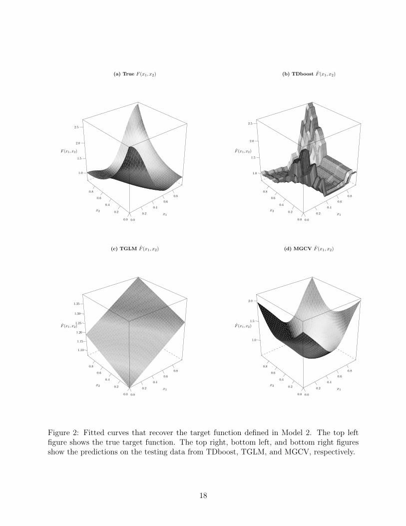
• Model 2 (Complex interaction): The target function has two hills and two valleys.

F (x1, x2) = e−5(1−x1)2+x22 + e−5x21+(1−x2)2 ,

which corresponds to a common scenario where the effect of one variable changes

depending on the effect of another. We assume x1, x2 ∼ Unif(0, 1), and y ∼ Tw(µ, φ, ρ)

with ρ = 1.5 and φ = 0.5.

We generate n = 1000 observations for training and n′ = 1000 for testing, and fit the

training data using TDboost, MGCV, and TGLM. Since the true target functions are known,

we consider the mean absolute deviation (MAD) as performance criteria,

MAD =1

n′

n′∑i=1

|F (xi)− F (xi)|,

where both the true predictor function F (xi) and the predicted function F (xi) are evaluated

on the test set. The resulting MADs on the testing data are reported in Table 1, which are

averaged over 100 independent replications. The fitted functions from Model 2 are plotted

in Figure 2. In both cases, we find that TDboost outperforms TGLM and MGCV in terms

of the ability to recover the true functions and gives the smallest prediction errors.

17

(a) True F (x1, x2)

0.0

0.2

0.4

0.6

0.8

0.0

0.2

0.4

0.6

0.8

1.0

1.5

2.0

2.5

x1

x2

F (x1, x2)

(b) TDboost F (x1, x2)

0.0

0.2

0.4

0.6

0.8

0.0

0.2

0.4

0.6

0.8

1.0

1.5

2.0

2.5

x1

x2

F (x1, x2)

(c) TGLM F (x1, x2)

0.0

0.2

0.4

0.6

0.8

0.0

0.2

0.4

0.6

0.8

1.10

1.15

1.20

1.25

1.30

1.35

x1

x2

F (x1, x2)

(d) MGCV F (x1, x2)

0.0

0.2

0.4

0.6

0.8

0.0

0.2

0.4

0.6

0.8

1.0

1.5

2.0

x1

x2

F (x1, x2)

Figure 2: Fitted curves that recover the target function defined in Model 2. The top leftfigure shows the true target function. The top right, bottom left, and bottom right figuresshow the predictions on the testing data from TDboost, TGLM, and MGCV, respectively.

18

Model TGLM MGCV TDboost

1 0.1102 (0.0006) 0.0752 (0.0016) 0.0595 (0.0021)2 0.3516 (0.0009) 0.2511 (0.0004) 0.1034 (0.0008)

Table 1: The averaged MADs and the corresponding standard errors based on 100 indepen-dent replications.

5.2 Case II

The idea is to see the performance of the TDboost estimator and MGCV estimator on a

variety of very complicated, randomly generated predictor functions, and study how the size

of the training set, distribution settings and other characteristics of problems affect final

performance of the two methods. We use the “random function generator” (RFG) model by

Friedman (2001) in our simulation. The true target function F is randomly generated as a

linear expansion of functions {gk}20k=1:

F (x) =20∑k=1

bkgk(zk). (27)

Here each coefficient bk is a uniform random variable from Unif[−1, 1]. Each gk(zk) is a

function of zk, where zk is defined as a pk-sized subset of the ten-dimensional variable x in

the form

zk = {xψk(j)}pkj=1, (28)

where each ψk is an independent permutation of the integers {1, . . . , p}. The size pk is ran-

domly selected by min(b2.5 + rkc , p), where rk is generated from an exponential distribution

with mean 2. Hence the expected order of interactions presented in each gk(zk) is between

four and five. Each function gk(zk) is a pk-dimensional Gaussian function:

gk(zk) = exp{− 1

2(zk − uk)

ᵀVk(zk − uk)}, (29)

where each mean vector uk is randomly generated from N(0, Ipk). The pk × pk covariance

matrix Vk is defined by

Vk = UkDkUᵀk, (30)

where Uk is a random orthonormal matrix, Dk = diag{dk[1], . . . , dk[pk]}, and the square

root of each diagonal element√dk[j] is a uniform random variable from Unif[0.1, 2.0]. We

19

generate data {yi,xi}ni=1 according to

yi ∼ Tw(µi, φ, ρ), xi ∼ N(0, Ip), i = 1, . . . , n, (31)

where µi = exp{F (xi)}.

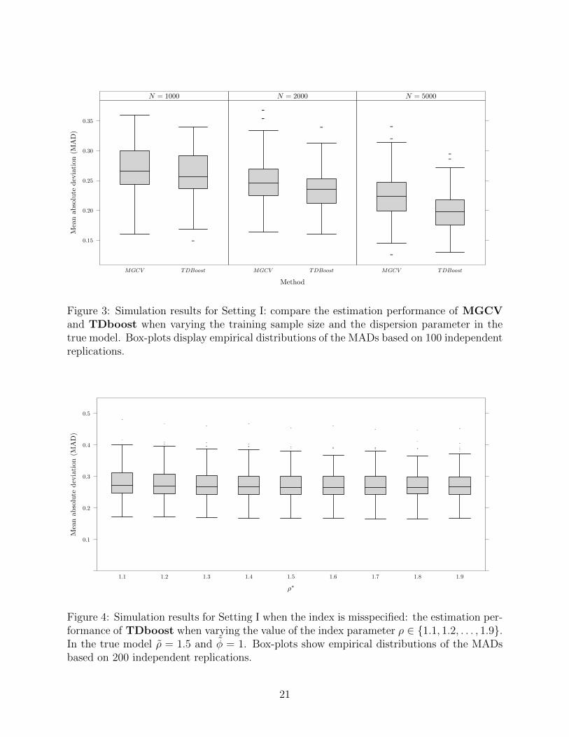
Setting I: when the index is known

Firstly, we study the situation that the true index parameter ρ is known when fitting models.

We generate data according to the RFG model with index parameter ρ = 1.5 and the

dispersion parameter φ = 1 in the true model. We set the number of predictors to be p = 10

and generate n ∈ {1000, 2000, 5000} observations as training sets, on which both MGCV

and TDboost are fitted with ρ specified to be the true value 1.5. An additional test set of

n′ = 5000 observations was generated for evaluating the performance of the final estimate.

Figure 3 shows simulation results for comparing the estimation performance of MGCV

and TDboost, when varying the training sample size. The empirical distributions of the

MADs shown as box-plots are based on 100 independent replications. We can see that in all

of the cases, TDboost outperforms MGCV in terms of prediction accuracy.

We also test estimation performance on µ when the index parameter ρ is misspecified,

that is, we use a guess value ρ differing from the true value ρ when fitting the TDboost model.

Because µ is statistically orthogonal to φ and ρ, meaning that the off-diagonal elements of

the Fisher information matrix are zero (Jørgensen, 1997), we expect µ will vary very slowly

as ρ changes. Indeed, using the previous simulation data with the true value ρ = 1.5 and

φ = 1, we fitted TDboost models with nine guess values of ρ ∈ {1.1, 1.2, . . . , 1.9}. The

resulting MADs are displayed in Figure 4, which shows the choice of the value ρ has almost

no significant effect on estimation accuracy of µ.

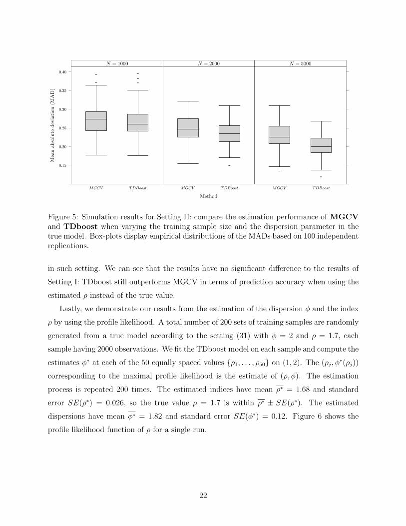
Setting II: using the estimated index

Next we study the situation that the true index parameter ρ is unknown, and we use the

estimated ρ obtained from the profile likelihood procedure discussed in Section 4.2 for fitting

the model. The same data generation scheme is adopted as in Setting I, except now both

MGCV and TDboost are fitted with ρ estimated by maximizing the profile likelihood. Figure

5 shows simulation results for comparing the estimation performance of MGCV and TDboost

20

Method

Meanabsolute

deviation(M

AD)

0.15

0.20

0.25

0.30

0.35

MGCV TDBoost

-

N = 1000

MGCV TDBoost

--

-

N = 2000

MGCV TDBoost

-

-

-

--

N = 5000

Figure 3: Simulation results for Setting I: compare the estimation performance of MGCVand TDboost when varying the training sample size and the dispersion parameter in thetrue model. Box-plots display empirical distributions of the MADs based on 100 independentreplications.

ρ∗

Meanab

solute

deviation

(MAD)

0.1

0.2

0.3

0.4

0.5

1.1 1.2 1.3 1.4 1.5 1.6 1.7 1.8 1.9

-

-

-

-

---

-

- --

-

- --

-

--

-

- --

-

- --

-

-

----

-

-

Figure 4: Simulation results for Setting I when the index is misspecified: the estimation per-formance of TDboost when varying the value of the index parameter ρ ∈ {1.1, 1.2, . . . , 1.9}.In the true model ρ = 1.5 and φ = 1. Box-plots show empirical distributions of the MADsbased on 200 independent replications.

21

Method

Meanabsolute

deviation(M

AD)

0.15

0.20

0.25

0.30

0.35

0.40

MGCV TDBoost

--

-

--

N = 1000

MGCV TDBoost

-

N = 2000

MGCV TDBoost

--

N = 5000

Figure 5: Simulation results for Setting II: compare the estimation performance of MGCVand TDboost when varying the training sample size and the dispersion parameter in thetrue model. Box-plots display empirical distributions of the MADs based on 100 independentreplications.

in such setting. We can see that the results have no significant difference to the results of

Setting I: TDboost still outperforms MGCV in terms of prediction accuracy when using the

estimated ρ instead of the true value.

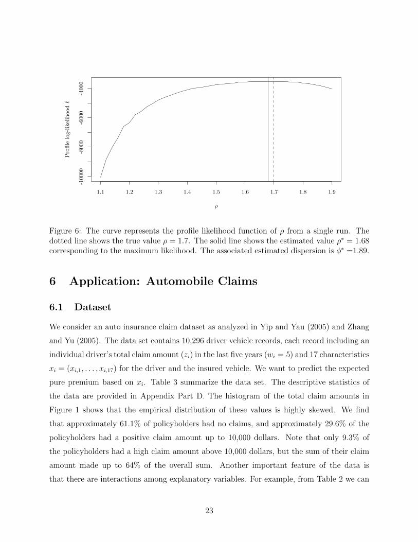
Lastly, we demonstrate our results from the estimation of the dispersion φ and the index

ρ by using the profile likelihood. A total number of 200 sets of training samples are randomly

generated from a true model according to the setting (31) with φ = 2 and ρ = 1.7, each

sample having 2000 observations. We fit the TDboost model on each sample and compute the

estimates φ∗ at each of the 50 equally spaced values {ρ1, . . . , ρ50} on (1, 2). The (ρj, φ∗(ρj))

corresponding to the maximal profile likelihood is the estimate of (ρ, φ). The estimation

process is repeated 200 times. The estimated indices have mean ρ∗ = 1.68 and standard

error SE(ρ∗) = 0.026, so the true value ρ = 1.7 is within ρ∗ ± SE(ρ∗). The estimated

dispersions have mean φ∗ = 1.82 and standard error SE(φ∗) = 0.12. Figure 6 shows the

profile likelihood function of ρ for a single run.

22

-10000

-800

0-6

000

-400

0

ρ

Pro

file

log-

like

lihood`

1.1 1.2 1.3 1.4 1.5 1.6 1.7 1.8 1.9

Figure 6: The curve represents the profile likelihood function of ρ from a single run. Thedotted line shows the true value ρ = 1.7. The solid line shows the estimated value ρ∗ = 1.68corresponding to the maximum likelihood. The associated estimated dispersion is φ∗ =1.89.

6 Application: Automobile Claims

6.1 Dataset

We consider an auto insurance claim dataset as analyzed in Yip and Yau (2005) and Zhang

and Yu (2005). The data set contains 10,296 driver vehicle records, each record including an

individual driver’s total claim amount (zi) in the last five years (wi = 5) and 17 characteristics

xi = (xi,1, . . . , xi,17) for the driver and the insured vehicle. We want to predict the expected

pure premium based on xi. Table 3 summarize the data set. The descriptive statistics of

the data are provided in Appendix Part D. The histogram of the total claim amounts in

Figure 1 shows that the empirical distribution of these values is highly skewed. We find

that approximately 61.1% of policyholders had no claims, and approximately 29.6% of the

policyholders had a positive claim amount up to 10,000 dollars. Note that only 9.3% of

the policyholders had a high claim amount above 10,000 dollars, but the sum of their claim

amount made up to 64% of the overall sum. Another important feature of the data is

that there are interactions among explanatory variables. For example, from Table 2 we can

23

AREA

Urban Rural

REVOKEDNo 3150.57 904.70Yes 14551.62 7624.36

Difference 11401.05 6719.66

Table 2: The averaged total claim amount for different categories of the policyholders.

ID Variable Type Description

1 AGE N Driver’s age

2 BLUEBOOK N Value of vehicle

3 HOMEKIDS N Number of children

4 KIDSDRIV N Number of driving children

5 MVR PTS N Motor vehicle record points

6 NPOLICY N Number of policies

7 RETAINED N Number of years as a customer

8 TRAVTIME N Distance to work

9 AREA C Home/work area: Rural, Urban

10 CAR USE C Vehicle use: Commercial, Private

11 CAR TYPE C Type of vehicle: Panel Truck, Pickup,Sedan, Sports Car, SUV, Van

12 GENDER C Driver’s gender: F, M

13 JOBCLASS C Unknown, Blue Collar, Clerical, Doctor,Home Maker, Lawyer, Manager, Professional, Student

14 MAX EDUC C Education level: High School or Below, Bachelors,High School, Masters, PhD

15 MARRIED C Married or not: Yes, No

16 REVOKED C Whether license revoked in past 7 years: Yes, No

Table 3: Explanatory variables in the claim history data set. Type N stands for numericalvariable, Type C stands for categorical variable.

see that the marginal effect of the variable REVOKED on the total claim amount is much

greater for the policyholders living in the urban area than those living in the rural area. The

importance of the interaction effects will be confirmed later in our data analysis.

6.2 Models

We separate the entire dataset into a training set and a testing set with equal size. Then

the TDboost model is fitted on the training set and tuned with five-fold cross validation.

24

For comparison, we also fit TGLM and MGCV, both of which are fitted using all the ex-

planatory variables. In MGCV, the numerical variables AGE, BLUEBOOK, HOMEKIDS,

KIDSDRIV, MVR PTS, NPOLICY, RETAINED and TRAVTIME are modeled by smooth

terms represented using penalized regression splines. We find the appropriate smoothness

for each applicable model term using Generalized Cross Validation (GCV) (Wahba, 1990).

For the TDboost model, it is not necessary to carry out data transformation, since the tree-

based boosting method can automatically handle different types of data. For other models,

we use logarithmic transformation on BLUEBOOK, i.e. log(BLUEBOOK), and scale all

the numerical variables except for HOMEKIDS, KIDSDRIV, MVR PTS and NPOLICY to

have mean 0 and standard deviation 1. We also create dummy variables for the categorical

variables with more than two levels (CAR TYPE, JOBCLASS and MAX EDUC). For all

models, we use the profile likelihood method to estimate the dispersion φ and the index ρ,

which are in turn used in fitting the final models.

6.3 Performance comparison

To examine the performance of TGLM, MGCV and TDboost, after fitting on the training set,

we predict the pure premium P (x) = µ(x) by applying each model on the independent held-

out testing set. However, attention must be paid when measuring the differences between

predicted premiums P (x) and real losses y on the testing data. The mean squared loss

or mean absolute loss is not appropriate here because the losses have high proportions of

zeros and are highly right skewed. Therefore an alternative statistical measure – the ordered

Lorenz curve and the associated Gini index – proposed by Frees et al. (2011) are used

for capturing the discrepancy between the premium and loss distributions. By calculating

the Gini index, the performance of different predictive models can be compared. Here we

only briefly explain the idea of the ordered Lorenz curve (Frees et al., 2011, 2013). Let

B(x) be the “base premium”, which is calculated using the existing premium prediction

model, and let P (x) be the “competing premium” calculated using an alternative premium

prediction model. In the ordered Lorenz curve, the distribution of losses and the distribution

of premiums are sorted based on the relative premium R(x) = P (x)/B(x). The ordered

premium distribution is

25

DP (s) =

∑ni=1B(xi)I(R(xi) ≤ s)∑n

i=1 B(xi),

and the ordered loss distribution is

DL(s) =

∑ni=1 yiI(R(xi) ≤ s)∑n

i=1 yi.

Two empirical distributions are based on the same sort order, which makes it possible to

compare the premium and loss distributions for the same policyholder group. The ordered

Lorenz curve is the graph of (DP (s), DL(s)). When the percentage of losses equals the

percentage of premiums for the insurer, the curve results in a 45-degree line, known as “the

line of equality”. Twice the area between the ordered Lorenz curve and the line of equality

measures the discrepancy between the premium and loss distributions, and is defined as the

Gini index. Curves below the line of equality indicate that, given knowledge of the relative

premium, an insurer could identify the profitable contracts, whose premiums are greater

than losses. Therefore, a larger Gini index (hence a larger area between the line of equality

and the curve below) would imply a more favorable model.

Following Frees et al. (2013), we successively specify the prediction from each model as

the base premium B(x) and use predictions from the remaining models as the competing

premium P (x) to compute the Gini indices. The entire procedure of the data splitting and

Gini index computation are repeated 20 times, and a matrix of the averaged Gini indices

and standard errors is reported in Table 4. To pick the “best” model, we use a “minimax”

strategy (Frees et al., 2013) to select the base premium model that are least vulnerable to

competing premium models; that is, we select the model that provides the smallest of the

maximal Gini indices, taken over competing premiums. We find that the maximal Gini index

is 15.528 when using B(x) = µTGLM(x) as the base premium, 12.979 when B(x) = µMGCV(x),

and 4.000 when B(x) = µTDboost(x). Therefore, TDboost has the smallest maximum Gini

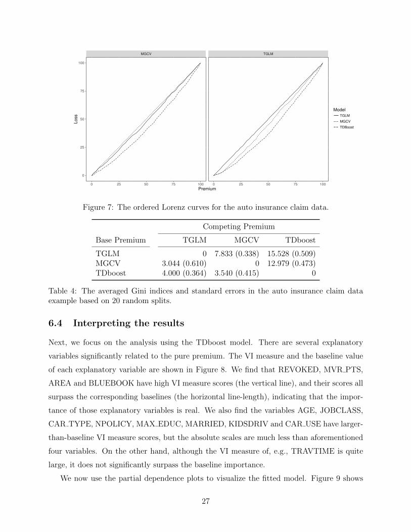
index at 4.000, hence is the least vulnerable to alternative scores. Figure 7 also shows that

when TGLM (or MGCV) is selected as the base premium, the area between the line of

equality and the ordered Lorenz curve is larger when choosing TDboost as the competing

premium, indicating again that the TDboost model represents the most favorable choice.

26

MGCV TGLM

0

25

50

75

100

0 25 50 75 100 0 25 50 75 100Premium

Loss

ModelTGLM

MGCV

TDBoost

Figure 7: The ordered Lorenz curves for the auto insurance claim data.

Competing Premium

Base Premium TGLM MGCV TDboost

TGLM 0 7.833 (0.338) 15.528 (0.509)MGCV 3.044 (0.610) 0 12.979 (0.473)TDboost 4.000 (0.364) 3.540 (0.415) 0

Table 4: The averaged Gini indices and standard errors in the auto insurance claim dataexample based on 20 random splits.

6.4 Interpreting the results

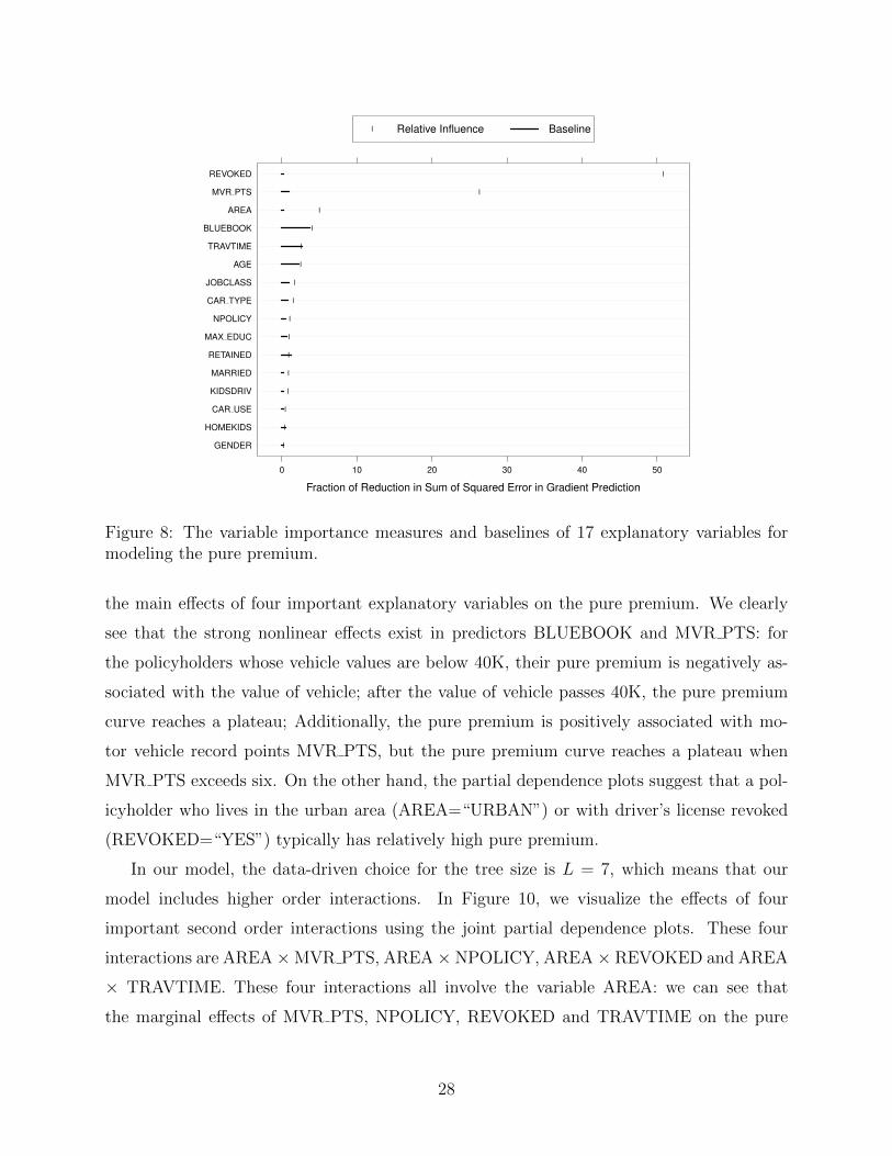
Next, we focus on the analysis using the TDboost model. There are several explanatory

variables significantly related to the pure premium. The VI measure and the baseline value

of each explanatory variable are shown in Figure 8. We find that REVOKED, MVR PTS,

AREA and BLUEBOOK have high VI measure scores (the vertical line), and their scores all

surpass the corresponding baselines (the horizontal line-length), indicating that the impor-

tance of those explanatory variables is real. We also find the variables AGE, JOBCLASS,

CAR TYPE, NPOLICY, MAX EDUC, MARRIED, KIDSDRIV and CAR USE have larger-

than-baseline VI measure scores, but the absolute scales are much less than aforementioned

four variables. On the other hand, although the VI measure of, e.g., TRAVTIME is quite

large, it does not significantly surpass the baseline importance.

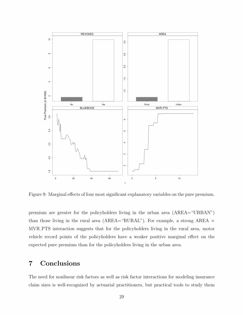
We now use the partial dependence plots to visualize the fitted model. Figure 9 shows

27

Fraction of Reduction in Sum of Squared Error in Gradient Prediction

GENDER

HOMEKIDS

CAR USE

KIDSDRIV

MARRIED

RETAINED

MAX EDUC

NPOLICY

CAR TYPE

JOBCLASS

AGE

TRAVTIME

BLUEBOOK

AREA

MVR PTS

REVOKED

0 10 20 30 40 50

l

l

l

l

l

l

l

l

l

l

l

l

l

l

l

l

l Relative Influence Baseline

Figure 8: The variable importance measures and baselines of 17 explanatory variables formodeling the pure premium.

the main effects of four important explanatory variables on the pure premium. We clearly

see that the strong nonlinear effects exist in predictors BLUEBOOK and MVR PTS: for

the policyholders whose vehicle values are below 40K, their pure premium is negatively as-

sociated with the value of vehicle; after the value of vehicle passes 40K, the pure premium

curve reaches a plateau; Additionally, the pure premium is positively associated with mo-

tor vehicle record points MVR PTS, but the pure premium curve reaches a plateau when

MVR PTS exceeds six. On the other hand, the partial dependence plots suggest that a pol-

icyholder who lives in the urban area (AREA=“URBAN”) or with driver’s license revoked

(REVOKED=“YES”) typically has relatively high pure premium.

In our model, the data-driven choice for the tree size is L = 7, which means that our

model includes higher order interactions. In Figure 10, we visualize the effects of four

important second order interactions using the joint partial dependence plots. These four

interactions are AREA×MVR PTS, AREA× NPOLICY, AREA× REVOKED and AREA

× TRAVTIME. These four interactions all involve the variable AREA: we can see that

the marginal effects of MVR PTS, NPOLICY, REVOKED and TRAVTIME on the pure

28

x

Pur

eP

rem

ium

(in$1

000)

1.8

2.0

2.2

2.4

2.6

0 20 40 60

BLUEBOOK

23

45

6

0 5 10

MVR PTS

24

68

10

No Yes

REVOKED

1.0

1.5

2.0

2.5

3.0

Rural Urban

AREA

Figure 9: Marginal effects of four most significant explanatory variables on the pure premium.

premium are greater for the policyholders living in the urban area (AREA=“URBAN”)

than those living in the rural area (AREA=“RURAL”). For example, a strong AREA ×MVR PTS interaction suggests that for the policyholders living in the rural area, motor

vehicle record points of the policyholders have a weaker positive marginal effect on the

expected pure premium than for the policyholders living in the urban area.

7 Conclusions

The need for nonlinear risk factors as well as risk factor interactions for modeling insurance

claim sizes is well-recognized by actuarial practitioners, but practical tools to study them

29

(a)

Rural

Urban

0

2

4

6

8

10

12

1

2

3

4

5

6

AREA

MVR PTS

µ(x)

(b)

Rural

Urban

2

4

6

8

0.5

1.0

1.5

2.0

2.5

AREA

NPOLICY

µ(x)

(c)

Rural

Urban

No

Yes

2

4

6

8

10

AREA

REVOKED

µ(x)

(d)

Rural

Urban

2040

6080

100120

140

0.5

1.0

1.5

2.0

2.5

3.0

AREA

TRAVTIME

µ(x)

Figure 10: Four strong pairwise interactions.

30

are very limited. In this paper, relying on neither the linear assumption nor a pre-specified

interaction structure, a flexible tree-based gradient boosting method is designed for the

Tweedie model. We implement the proposed method in a user-friendly R package “TDboost”

that can make accurate insurance premium predictions for complex data sets and serve as a

convenient tool for actuarial practitioners to investigate the nonlinear and interaction effects.

In the context of personal auto insurance, we implicitly use the policy duration as a volume

measure (or exposure), and demonstrate the favorable prediction performance of TDboost

for the pure premium. In cases that exposure measures other than duration are used, which is

common in commercial insurance, we can extend the TDboost method to the corresponding

claim size by simply replacing the duration with any chosen exposure measure.

TDboost can also be an important complement to the traditional GLM model in insurance

rating. Even under the strict circumstances that the regulators demand the final model to

have a GLM structure, our approach can still be quite helpful due to its ability to extract

additional information such as non-monotonicity/non-linearity and important interaction.

In Appendix Part E, we provide an additional real data analysis to demonstrate that our

method can provide insights into the structure of interaction terms. After integrating the

obtained information about the interaction terms into the original GLM model, we can much

enhance the overall accuracy of the insurance premium prediction while maintaining a GLM

model structure.

In addition, it is worth mentioning that the applications of the proposed method can

go beyond the insurance premium prediction and be of interest to researchers in many

other fields including ecology (Foster and Bravington, 2013), meteorology (Dunn, 2004)

and political science (Lauderdale, 2012). See, for example, Dunn and Smyth (2005) and

Qian et al. (2015) for descriptions of the broad Tweedie distribution applications. The

proposed method and the implementation tool allow researchers in these related fields to

venture outside the Tweedie GLM modeling framework, build new flexible models from

nonparametric perspectives, and use the model interpretation tools demonstrated in our real

data analysis to study their own problems of interests.

31

References

Anstey, K. J., Wood, J., Lord, S., and Walker, J. G. (2005), “Cognitive, sensory and physical

factors enabling driving safety in older adults,” Clinical psychology review, 25, 45–65.

Breiman, L. (1996), “Bagging predictors,” Machine learning, 24, 123–140.

— (1998), “Arcing classifier (with discussion and a rejoinder by the author),” The Annals

of Statistics, 26, 801–849.

— (1999), “Prediction games and arcing algorithms,” Neural Computation, 11, 1493–1517.

Breiman, L., Friedman, J., Olshen, R., Stone, C., Steinberg, D., and Colla, P. (1984),

“CART: Classification and regression trees,” Wadsworth.

Brent, R. P. (2013), Algorithms for minimization without derivatives, Courier Dover Publi-

cations.

Buhlmann, P. and Hothorn, T. (2007), “Boosting algorithms: Regularization, prediction and

model fitting,” Statistical Science, 22, 477–505.

Dionne, G., Gourieroux, C., and Vanasse, C. (2001), “Testing for evidence of adverse selection

in the automobile insurance market: A comment,” Journal of Political Economy, 109, 444–

453.

Dunn, P. K. (2004), “Occurrence and quantity of precipitation can be modelled simultane-

ously,” International Journal of Climatology, 24, 1231–1239.

Dunn, P. K. and Smyth, G. K. (2005), “Series evaluation of Tweedie exponential dispersion

model densities,” Statistics and Computing, 15, 267–280.

Elith, J., Leathwick, J. R., and Hastie, T. (2008), “A working guide to boosted regression

trees,” Journal of Animal Ecology, 77, 802–813.

Foster, S. D. and Bravington, M. V. (2013), “A Poisson–Gamma model for analysis of

ecological non-negative continuous data,” Environmental and ecological statistics, 20, 533–

552.

32

Frees, E. W., Meyers, G., and Cummings, A. D. (2011), “Summarizing insurance scores

using a Gini index,” Journal of the American Statistical Association, 106.

Frees, E. W. J., Meyers, G., and Cummings, A. D. (2013), “Insurance ratemaking and a

Gini index,” Journal of Risk and Insurance.

Freund, Y. and Schapire, R. (1997), “A decision-theoretic generalization of on-line learning

and an application to boosting,” Journal of Computer and System Sciences, 55, 119–139.

Friedman, J. (2001), “Greedy function approximation: A gradient boosting machine,” The

Annals of Statistics, 29, 1189–1232.

Friedman, J., Hastie, T., and Tibshirani, R. (2000), “Additive logistic regression: A statis-

tical view of boosting (With discussion and a rejoinder by the authors),” The Annals of

Statistics, 28, 337–407.

Friedman, J. H. (2002), “Stochastic gradient boosting,” Computational Statistics & Data

Analysis, 38, 367–378.

Haberman, S. and Renshaw, A. E. (1996), “Generalized linear models and actuarial science,”

Statistician, 45, 407–436.

Hastie, T., Tibshirani, R., and Friedman, J. (2009), The elements of statistical learning: Data

mining, inference, and prediction. Second Edition., Springer Series in Statistics, Springer.

Hastie, T. J. and Tibshirani, R. J. (1990), Generalized additive models, vol. 43, CRC Press.

Jørgensen, B. (1987), “Exponential dispersion models,” Journal of the Royal Statistical So-

ciety. Series B (Methodological), 127–162.

— (1997), The theory of dispersion models, vol. 76, CRC Press.

Jørgensen, B. and de Souza, M. C. (1994), “Fitting Tweedie’s compound Poisson model to

insurance claims data,” Scandinavian Actuarial Journal, 1994, 69–93.

Lauderdale, B. E. (2012), “Compound Poisson–Gamma regression models for dollar out-

comes that are sometimes zero,” Political Analysis, 20, 387–399.

33

Mildenhall, S. J. (1999), “A systematic relationship between minimum bias and generalized

linear models,” in Proceedings of the Casualty Actuarial Society, vol. 86, pp. 393–487.

Murphy, K. P., Brockman, M. J., and Lee, P. K. (2000), “Using generalized linear models

to build dynamic pricing systems,” in Casualty Actuarial Society Forum, Winter, pp.

107–139.

Nelder, J. and Wedderburn, R. (1972), “Generalized Linear Models,” Journal of the Royal

Statistical Society. Series A (General), 135, 370–384.

Ohlsson, E. and Johansson, B. (2010), Non-life insurance pricing with generalized linear

models, Springer.

Peters, G. W., Shevchenko, P. V., and Wuthrich, M. V. (2008), “Model risk in claims

reserving within Tweedie’s compound Poisson models,” ASTIN Bulletin, to appear.

Qian, W., Yang, Y., and Zou, H. (2015), “Tweedie’s compound Poisson model with grouped

elastic net,” Journal of Computational and Graphical Statistics, preprint.

Renshaw, A. E. (1994), “Modelling the claims process in the presence of covariates,” ASTIN

Bulletin, 24, 265–285.

Ridgeway, G. (2007), “Generalized Boosted Regression Models,” R package manual.

Sandri, M. and Zuccolotto, P. (2008), “A bias correction algorithm for the Gini variable im-

portance measure in classification trees,” Journal of Computational and Graphical Statis-

tics, 17.

— (2010), “Analysis and correction of bias in Total Decrease in Node Impurity measures for

tree-based algorithms,” Statistics and Computing, 20, 393–407.

Showers, V. E. and Shotick, J. A. (1994), “The effects of household characteristics on demand

for insurance: A tobit analysis,” Journal of Risk and Insurance, 492–502.

Smyth, G. and Jørgensen, B. (2002), “Fitting Tweedie’s compound Poisson model to insur-

ance claims data: Dispersion modelling,” ASTIN Bulletin, 32, 143–157.

34

Smyth, G. K. (1996), “Regression analysis of quantity data with exact zeros,” in Proceedings

of the second Australia–Japan workshop on stochastic models in engineering, technology

and management, Citeseer, pp. 572–580.

Tweedie, M. (1984), “An index which distinguishes between some important exponential

families,” in Statistics: Applications and New Directions: Proc. Indian Statistical Institute

Golden Jubilee International Conference, pp. 579–604.

Van de Ven, W. and van Praag, B. M. (1981), “Risk aversion and deductibles in private health

insurance: Application of an adjusted tobit model to family health care expenditures,”

Health, economics, and health economics, 125–48.

Wahba, G. (1990), Spline models for observational data, vol. 59, SIAM.

White, A. P. and Liu, W. Z. (1994), “Technical note: Bias in information-based measures in

decision tree induction,” Machine Learning, 15, 321–329.

Wood, S. (2001), “mgcv: GAMs and generalized ridge regression for R,” R News, 1, 20–25.

— (2006), Generalized additive models: An introduction with R, CRC press.

Yip, K. C. and Yau, K. K. (2005), “On modeling claim frequency data in general insurance

with extra zeros,” Insurance: Mathematics and Economics, 36, 153–163.

Zhang, T. and Yu, B. (2005), “Boosting with early stopping: Convergence and consistency,”

The Annals of Statistics, 1538–1579.

Zhang, W. (2011), “cplm: Monte Carlo EM algorithms and Bayesian methods for fitting

Tweedie compound Poisson linear models,” R package, http://cran.r-project.org/

web/packages/cplm/index.html.

35