Laboratoire de Mathématiques, UMR CNRS 5127

Université de Savoie, 73376 Le Bourget du Lac, France

Mémoire présenté à l'Université de Savoie

en vue d'obtenir une Habilitation à Diriger des Recherches

présenté par Belkacem SAID-HOUARI

Spécialité Mathématiques appliquées

Soutenue le 10 Décembre 2009 devant le jury composé de :

• Didier Bresch, Université de Savoie, Examinateur

• Nicolas Burq, Université Paris-Sud 11 et Institut Universitaire de France, Rapporteur

• Arnaud Münch, Université Blaise Pascal, Clermont-Ferrand, Examinateur

• Mokthar Kirane, Université de la Rochelle, Rapporteur

• Reinhard Racke, Université de Constance, Allemagne, Rapporteur

Etude de quelques problèmes d'évolution non linéaires de type

hyperbolique : existence, unicité et comportement asymptotique.

Table des matières

I Curriculum Vitæ 1

II Synthèse des activités de recherche 9

1 Introduction 111.1 Semi-linear wave equations . . . . . . . . . . . . . . . . . . . . . . . . . . . . . . . . . . 111.2 The wave equations with dynamic boundary conditions . . . . . . . . . . . . . . . . . . 171.3 Nonclassical thermoelasticity . . . . . . . . . . . . . . . . . . . . . . . . . . . . . . . . 181.4 Timoshenko systems . . . . . . . . . . . . . . . . . . . . . . . . . . . . . . . . . . . . . 20

2 Semi-linear wave equations 242.1 Viscoelastic wave equation . . . . . . . . . . . . . . . . . . . . . . . . . . . . . . . . . . 242.2 System of nonlinear wave equations . . . . . . . . . . . . . . . . . . . . . . . . . . . . . 262.3 Boussinesq equation . . . . . . . . . . . . . . . . . . . . . . . . . . . . . . . . . . . . . 292.4 Kirchho-type wave equation . . . . . . . . . . . . . . . . . . . . . . . . . . . . . . . . 322.5 The wave equations with fractional damping . . . . . . . . . . . . . . . . . . . . . . . . 33

3 The wave equations with dynamic boundary conditions 363.1 Local existence . . . . . . . . . . . . . . . . . . . . . . . . . . . . . . . . . . . . . . . . 383.2 Asymptotic stability . . . . . . . . . . . . . . . . . . . . . . . . . . . . . . . . . . . . . 413.3 Exponential growth . . . . . . . . . . . . . . . . . . . . . . . . . . . . . . . . . . . . . . 443.4 Blow up . . . . . . . . . . . . . . . . . . . . . . . . . . . . . . . . . . . . . . . . . . . . 45

4 Nonclassical thermoelasticity 464.1 Thermoelasticity of second sound . . . . . . . . . . . . . . . . . . . . . . . . . . . . . . 464.2 Thermoelasticity of type III . . . . . . . . . . . . . . . . . . . . . . . . . . . . . . . . . 524.3 Transmission problem in thermoelasticity of type III . . . . . . . . . . . . . . . . . . . 56

5 Timoshenko-type systems 605.1 Timoshenko-type systems in thermoelasticity of second sound . . . . . . . . . . . . . . 605.2 Timoshenko-type system in thermoelasticity of type III . . . . . . . . . . . . . . . . . . 705.3 Timoshenko-type system with history in thermoelasticity of type III . . . . . . . . . . 72

Acknowledgement

• First of all, I am very grateful to Dr. Nasser Eddine Tatar, because he was my rst advisor inthis area of research since 2001, when I was student in Master "Magester" at Annaba University(Algeria).• Huge thanks to my PhD advisor : Prof. Salim Messaoudi, for his guidance, encouragement andcontinuous support through my research. I am very grateful to him.• I especially thank Prof. Mokhtar Kirane for all his help not only for me but for many Algerianstudents and laboratories. Also, I would like to thank him for having accepted to be member of thejury.• I would like to thank deeply my collaborator at Savoie University : Dr. Stéphane Gerbi, forproviding me ideas of what to include in this thesis and for having been so kind to revise this thesiswith great care. This work would be incomplete and incorrect without his help.

Besides my advisors, I would like to thank the rest of my thesis committee.• My sincere thanks to the other two reviewers : Prof. Nicolas Burq (Université Paris-Sud 11 etInstitut Universitaire de France) and Prof. Reinhard Racke (University of Konstanz, Germany)for their careful reading of the material presented in this thesis.• I also wish to thank Prof. Didier Bresch (Université de Savoie) and Prof. Arnaud Münch(Université Blaise Pascal, Clermont-Ferrand) for their acceptance to be part of the jury.• I would also like to thank Dr. Abdellah Chalabi for his helps and suggestions during my stay atToulouse as Post-Doc student.• I am especially indebted to the members of Lab of Math of Savoie University for their support overthe year.• I must thank the members of the Mathematic department of Annaba University (Algeria) includingthe collogues, stas and students.• I owe my loving thanks to my wife Nadia for being incredibly understanding and supportive.• Finally, this work is dedicated to my dear parents, for their love and encouragement during the pastyears.

Belkacem.

Première partie

Curriculum Vitæ

1

Etat civil

Belkacem SAID-HOUARINé le 25 février 1978, à Arib, AlgérieNationalité AlgérienneMarié, sans enfants.

Adresse personnelle

84 Rue Balzac, Apt 1473000 ChambéryFrance

Adresse professionnelle

1. Laboratoire de Mathématiques,Université de Savoie,73376 Le Bourget du LacFranceTél : (+33) 04 79 75 85 85

2. Laboratoire de Mathématiques Appliquées,Université Badji Mokhtar,B.P. 12 Annaba 23000Algériee-mail : saidhouarib@yahoo.fr

Situations professionnelles

• 2009 : Qualié à la fonction de Maître de Conférences en section 26.• 2009- : Post Doctorant au Laboratoire de Mathématiques Université de Savoie.Bourse Région Rhône Alpes de 12 mois à partir de Avril 2009.• 2008-2009 : Post Doctorant à l'Institut de Mathématiques de Toulouse, MIP.Bourse ERASMUS-MUNDUS de 10 mois à partir de Juin 2008.• 2002-2008 : Maitre assistant à l'Université de Annaba, au Université de Skikda et au centre Uni-versitaire de Souk-Ahras, Algérie.

Formation

• 2002-2005 : Thése de Doctorat, Université de Annaba (Algérie). Mention très honorable.Thermoelasticitè non classique , soutenue le 29 Novembre 2005 à l'Université de Annaba.Jury : S. A. Messaoudi (King Fahd University of Petroleum and Minerals, Arabie Saoudite, rap-porteur), F. Rebbani (Université d'Annaba, Présidente), A. Aibeche (Université de Setif, Algérie),M. Denche (Université de Constantine, Algérie), B. Khodja (Université d'Annaba), S. Mazouzi (Uni-versité d'Annaba).• 2000-2002 : Thèse de Magister, mention Bien, à l'Université d'Annaba, sous la direction deN.E. Tatar : Etude de l'iteraction entre un terme dissipatif et un terme source dans un problèmehyperbolique.• 1996-2000 : DES en Mathématiques, option Analyse fonctionelle, Université de Blida (Algérie).

3

Activitè de recherche

Thémes de recherche

• Comportement qualitatif des équations des ondes amorties et conditions aux limites dynamiques,• Système de thermoélasticité non classique,• Théorie du contrôle des Equations aux Dérivées Partielles,• Lois de conservation.

Publications

• 16 articles parus ou à paraître dans des revues internationales avec comité de lecture• 8 articles soumis à des revues internationales avec comité de lecture• 4 articles en préparation• 3 publications dans les actes de congrès internationaux à comité de lecture

Encadrements de thèses

• Co-encadrement (80 %) avec Hocine Sissaoui (Professeur, Université d'Annaba) de la thèse de Ma-gister de Khaled Zennir : Comportement asymptotique de quelques problemes de visco-élasticité.,Soutenance Février 2009.• Co-encadrement (80 %) avec Hocine Sissaoui (Professeur, Université d'Annaba) de la thèse de Doc-torat de Ouchenane Djamel : Comportements asymptotiques de quelques problèmes des milieuxporeux, Début : Octobre 2008.

Divers et invitations à l'étranger

• Referee pour Survey in Mathematics and its Applications, European Journal of Mechanics - A/Solids, Acta Mathematica Sinica, Nonlinear Analysis, Journal of Mathemtical Physics.• Octobre 2008 : Invitation d'un mois au Laboratoire de Mathématiques de l'Université de Savoie,contact : Stéphane Gerbi.• Mai 2008 : Invitation d'un mois au Laboratoire de Mathématiques de l'Université de Savoie, contact :Stéphane Gerbi.• Janvier 2008 : Invitation de 10 jours Laboratoire de Mathématiques de l'Université de Savoie,contact : Stéphane Gerbi.

Activité d'enseignement

Cours, travaux dirigés

Université de Annaba, (Algérie) (2007-)• Travaux dirigés de Licence de Mathématiques : Analyse réelle, Algèbre générale, et Algèbre linéaire.• Travaux dirigés de Licence d'Économie : Analyse réelle, Algèbre générale et Algèbre linéaire.

Université de Annaba, (Algérie) (2001-2003)

4

• Travaux dirigés de Licence de Sciences exactes, L1 : Algèbre générale et Algèbre linéaire.• Travaux dirigés de Licence de Sciences économiques, L1 : Mathématiques générales.

Université de Skikda, (Algérie)(2002-2007)

• Cours et Travaux dirigés de DES de Mathématiques, 4ème année : Analyse fonctionelle.• Cours et Travaux dirigés de DES de Mathématiques, 4ème année : Équations diérentielles ordi-naires.• Cours et Travaux dirigés de DES de Mathématiques, 3ème année : Mesure et Intégration.• Travaux dirigés de DES de Mathématiques, 1ère année : Algèbre générale et Algèbre linéaire.Centre Universitaire de Souk-Ahras, (Algérie)(2004-2006)

• Cours et Travaux dirigés de DES de Mathématiques, 4ème année : Analyse fonctionelle.• Cours et Travaux dirigés de DES de Mathématiques, 4ème année : Équations diérentielles ordi-naires.• Cours et Travaux dirigés de DES de Mathématiques, 2ème année : Topologie.• Cours et Travaux dirigés de DES de Mathématiques, 1ère année : Algèbre générale et Algèbrelinéaire.

Publications scientifiques détaillées

Articles publiés ou à paraître dans des revues internationales à comité de lecture

[1] B. Said-Houari, Blow-up of positive initial-energy solutions of system of nonlinear wave equationswith damping and source terms, Dierential and Integral Equations, 23, No. 1-2 (2010), pp 79-92.

[2] S. A. Messaoudi, B. Said-Houari, Global nonexistence of positive initial-energy solutions of asystem of nonlinear viscoelastic wave equations with damping and source terms, à paraître dansJournal of Mathematical Analysis and Applications, (2009), épreuve disponible à l'adressehttp://dx.doi.org/10.1016/j.jmaa.2009.10.050.

[3] S. Gerbi, B. Said-Houari , Asymptotic stability and blow up for a semilinear damped wave equationwith dynamic boundary conditions, à paraître dans Dierential and Integral Equations, (2009).

[4] S. A. Messaoudi, B. Said-Houari, Uniform decay in a Timoshenko-type system with past history,J. Math. Anal. Appl., No. 360, (2009), pp. 459-475.

[5] S. A. Messaoudi, B. Said-Houari, Energy decay in transmission problem in thermoelasticity oftype III, IMA Journal of Applied Mathematics, 74, No. 3, (2009), pp 344-360.

[6] B. Said-Houari, Convergence to strong nonlinear diusion waves for solutions to p-system withdamping, Journal of Dierential Equations, 247, No. 3, (2009), pp. 917-930.

[7] S. A. Messaoudi, Michael Pokojovy and B. Said-Houari, Nonlinear damped Timoshenko-type sys-tems with second sound- Global existence and exponential stability, Math. Meth. Appl. Sci. 32,Issue 5, (2009), pp. 505-534.

[8] S. A. Messaoudi, B. Said-Houari Energy decay in a Timoshenko-type system with history in ther-moelasticity of type III, Advances in Dierential Equations. Vol. 14, No. 3-4, (2009), pp. 375-400.

[9] S. Gerbi , B. Said-Houari, Local existence and exponential growth for a semilinear damped waveequation with dynamic boundary conditions, Advances in Dierential Equations, Vol. 13, No.11-12, (2008), pp. 1051-1074.

[10] S. A. Messaoudi, B. Said-Houari, Energy decay in a Timoshenko-type system of thermoelasticityof type III, J. Math. Anal. Appl, 348, Issue 1, (2008), pp. 1225-1237.

5

[11] S. A. Messaoudi, B. Said-Houari, N.E Tatar Global existence and asymptotic behavior for a frac-tional dierential equation., Appl. Math. Comput. 188 (2007), No. 2, pp. 1955-1962.

[12] S. A. Messaoudi, B. Said-Houari, A blow-up result for a higher-order nonlinear Kirchho-typehyperbolic equation., Appl. Math. Lett. 20 (2007), No. 8, pp. 866-871.

[13] S. A. Messaoudi, B. Said-Houari, A global nonexistence result for the nonlinearly damped multi-dimensional Boussinesq equation., Arab. J. Sci. Eng. Sect. A Sci. 31 (2006), No. 1, pp. 57-68.

[14] S. A. Messaoudi, B. Said-Houari, Exponential stability in one-dimensional non-linear thermoe-lasticity with second sound., Math. Methods Appl. Sci. 28 (2005), No. 2, pp. 205-232.

[15] S. A. Messaoudi, B. Said-Houari, Global non-existence of solutions of a class of wave equationswith non-linear damping and source terms., Math. Methods Appl. Sci. 27 (2004), No. 14, pp.1687-1696.

[16] S. A. Messaoudi, B. Said-Houari, Blowup of solutions with positive energy in nonlinear thermoe-lasticity with second sound., J. Appl. Math. (2004), No. 3, pp. 201-211.

Articles soumis

[soum1] B. Said-Houari, Energy decay in thermoelasticity with second sound, (2008).

[soum2] S. A. Messaoudi, B. Said-Houari, Energy decay in a Timoshenko-type system with history inthermoelasticity of second sound, (2008).

[soum3] S. Gerbi, B. Said-Houari, Exponential decay for solutions to semilinear damped wave equation,(2009).

[soum4] S. A. Messaoudi, B. Said-Houari, Exponential stability in nonlinear one dimensional thermoelas-ticity of type III, (2009).

[soum5] B. Said-Houari, Existence and decay of solutions of a nonlinear system of wave equations, (2009).

[soum6] B. Said-Houari, Exponential growth of positive initial-energy solutions of a system of nonlinearviscoelastic wave equations with damping and source terms, (2009).

[soum7] B. Said-Houari, Stability result of the Timoshenko system with time-varying delay term in theinternal feedbacks, (2009).

[soum8] B. Said-Houari, Y. Laskri, Stability result of the Timoshenko system with a delay term in theinternal feedback, (2009).

Articles en préparation

[prep1] S. Gerbi, B. Said-Houari, Asymptotic behavior of the wave equation with dynamic boundary condi-tions and a damping with time delay, (2009).

[prep2] S. Gerbi , B. Said-Houari, Blow-up of the wave equation with a nonlinear dissipation of cubicconvolution in RN , (2009).

[prep3] B. Said-Houari, A blow up with positive initial energy of solutions of a class of wave equationswith nonlinear damping and source terms, (2009).

[prep4] B. Said-Houari, S.A. Messaoudi, B. Guesmia, Existence and general decay of solutions of a non-linear system of viscoelastic equations, (2009).

6

Rapports non publiés, thèse.

[1] S. A. Messaoudi, B. Said-Houari, Boundary stabilization of a system of thermoelasticity type III,The fourth UAE Math Day, April 27, 2006, Sharjah, UAE.

[2] S. A. Messaoudi, B. Said-Houari, A decay result in a system of thermo-elasticity type III, Pro-ceedings of the UAE Math-Day, Nova Publishing Company, New York. 2005.

[3] B. Said-Houari, Nonclassical thermoelasticity, thèse de Doctorat, Université de Annaba (Algérie),2005.

[4] B. Said-Houari, Etude de l'iteraction entre un terme dissipative et un terme source dans unproblème hyperbolique, thèse de Magistère, Université de Annaba (Algérie), 2002.

[5] B. Said-Houari, N. E. Tatar Etude de l'interaction entre un terme dissipative et un terme sourcedans un problème hyperbolique, (RAMA 3 Mai 2002, Algérie),

Conférences dans des séminaires et congrès

• Séminaire au LATP, Université de Marseille, 6 Octobre 2009.

• Colloque international : Aspects géométriques des équations aux dérivées partielles, CIRM,Luminy, 2 au 6 mars 2009.

• Colloque international : Contrôle et Problèmes Inverses pour les EDP : Aspects Théoriques etNumériques, CIRM, Luminy, 16 au 20 février 2009.

• Colloque international sur les équations aux dérivées partielles et leurs applications, Algérie,(2007).

• 2èmes Journées d'Equations Diérentielles et leurs Applications, Algérie, (2006).

• Journées sur les équations diérentielles et leurs applications, Algérie, (2002).

• RAMA 3 (3ème Rencontre Algérienne de Mathématiques Appliquées), Algérie, (2002).

• Plusieurs séminaires en Algérie et en France.

7

Deuxième partie

Synthèse des activités de recherche

9

1 Introduction

The study of the asymptotic behavior of solutions of nonlinear evolution equations, particularly thosegoverning gas dynamics, quantum theory and thermoelasticity, has been an important area for theinteraction between the partial dierential equations and physics.A wide class of problems of great importance in physics and engineering are formulated in terms ofnonlinear evolution equations. A general form of such equations is written as

∂u

∂t= Au+ F (u)

where the nonlinear operator A, its domain D(A) (the space of functions on which it acts) and thefunction F are all specied by the nature of the problem.For example, if A = ∆, we obtain the heat equation, whereas the wave equation is obtained whenU = (u, ut) and A is the matrix

A =

(0 I∆ 0

).

For the Schrödinger equation, A = i(∆ + V ) where V (x) is a potential function.The study of hyperbolic problems has interested many mathematicians during the past decades. Al-though a lot of challenging problems have already been solved, there are still many open questionseven in the case of the simplest model.

My research interests are divided into ve main parts : Semi-linear wave equations, The wave equations with dynamic boundary conditions, Nonclassical thermoelasticity, Timoshenko systems, Conservation laws.

In the references cited all along this introduction, the bold ones are part of my publications.

1.1 Semi-linear wave equations

The nonlinear wave equations may come from the modelizaton continuous media such as vibratingstrings, elasticity and uid ows.For example the one dimensional wave equation

utt = uxx

was introduced and analyzed by d'Alembert as a model of the vibrating string.Also, two and three dimensional wave equations

utt = ∆u

was studied by Bernoulli as a model of acoustic waves.

11

I have been interested in this type of problems since my Master thesis [118]. In that thesis, withDr. Tatar (KFUPM), I worked on some hyperbolic equations. I studied the interaction between thedissipative term of the form g(ut) and a source term f(u) in various type of wave equations. I lookedto the problem of existence of classical as well as weak solutions by using the Galekin approximationscombined with the xed point theorem. I also studied the qualitative behavior of the solutions : decayrate and the blow up in nite time.I continued the study of this kind of problems in my Ph.D. thesis [68, 69], with Prof. Messaoudi(KFUPM), I established many results concerning the asymptotic behavior and the blow up of solutionsof dierent semi-linear wave equation.Our work improved earlier results. For this reason, these results have been published in internationaljournals such as : Mathematical Methods in Applied Sciences, The Arabian Journal of Engineering and Sciences, Journal of Applied Mathematics, Journal of Applied Math Letters, Journal of Applied Mathematics and Computations, Journal of Mathematical Analysis and Applications, Advances in Dierential Equations, Journal of Dierential Equations, Dierential and Integral equations.

Viscoelastic wave equation

The characterization of situations where blow up actually occurs is one of the most important questionsin the theory of nonlinear equation of evolution. We considered in [68] the following initial boundaryvalue problem

utt −∆ut − div(|∇u|α−2∇u

)− div

(|∇ut|β−2∇ut

)+a |ut|m−2 ut = b |u|p−2 u, x ∈ Ω, t > 0 (1.1)

with the following initial and boundary conditions

u (x, 0) = u0 (x) , ut (x, 0) = u1 (x) , x ∈ Ω,

u (x, t) = 0, x ∈ ∂Ω, t > 0 (1.2)

where a, b > 0, α, β, m, p > 2, and Ω is a bounded domain of RN (N ≥ 1), with a smooth boundary∂Ω.Equation (1.1) appears in the model of the nonlinear viscoelasticity (See [144] and reference therein).It can also be considered as a system governing the longitudinal motion of a viscoelastic congurationobeying a nonlinear Voigt model.In the absence of viscosity and strong damping, equation (1.1) becomes

utt − div(|∇u|α−2∇u

)+ a |ut|m−2 ut = b |u|p−2 u, x ∈ Ω, t > 0. (1.3)

12

For b = 0, it is well known that the damping term a |ut|m−2 ut assures global existence and decay ofthe solution energy for any arbitrary initial data in the energy space (see [39], [51]).For a = 0, the source term b |u|p−2 u causes nite time blow up of solutions with negative initialenergy if p > α (see [10] and [46]). The interaction between the damping and the source terms wasrst considered by Levine [57, 58] in the linear damping case (α = m = 2). He showed that solutionswith negative initial energy blow up in nite time. The basic idea in [57, 58] is to construct a positivefunctional L(t) of the solution and show that for some γ > 0, the function L−γ(t) is a positive concavefunction of t. In order to nd such γ, it is sucient to verify that :

d2L−γ(t)

dt2= −γL−γ−2(t)

[LL

′′ − (1 + γ)L′2

(t)]≤ 0 , ∀t ≥ 0 .

This is equivalent to prove that L(t) satises the dierential inequality

LL′′ − (1 + γ)L

′2(t) ≥ 0 , ∀t ≥ 0.

Georgiev and Todorova in their famous paper [29], extended Levine's result to the nonlinear dampingcase (m > 2). In their work, the authors considered (1.3) with α = 2 and introduced a method dierentthan the one known as the concavity method. They determined suitable relations between m and p,for which there is global existence or alternatively nite time blow up. Precisely, they showed thatsolutions continue to exist globally in time if m ≥ p and blow up in nite time if p > m and theinitial energy is suciently negative. This result was later generalized to an abstract setting and tounbounded domains by Levine and Serrin [55] and Levine, Park, and Serrin [54]. In these papers,the authors showed that no solution with negative energy can be extended on [0, ∞) if p > m andproved several non continuation theorems. This generalization allowed them also to apply their resultto quasilinear situations (α > 2). Vitillaro [140] combined the arguments in [29] and [55] to extendthese results to certain situations where the damping is nonlinear and the solution has positive initialenergy. Similar results have also been established by Todorova [134] for dierent Cauchy problems.In [144], Yang studied (1.1)-(1.2) and proved a blow up result under the condition p > maxα,m,α > β, and the initial energy is suciently negative. In fact this condition made clear that there existsa certain relation between the blow-up time and |Ω|. We should note here that (1.1) corresponds toequation (5) of [144] but the same conclusions hold for equation (1) of the same paper, under suitableconditions, stated in theorem 2.3 of [144].In [68] we proved (with S. Messaoudi) that any solution of (1.1)-(1.2), with negative initial energy(large initial data), blows up in nite time if p > maxα,m, α > β. Therefore, our result improvesthe one of [144]. Our technique of proof follows closely the argument of [29]. This method based on theconstruction of a perturbed functional energy L(t) and show that L (t) satises a dierential inequalityof the form

L′(t) ≥ ξLq (t) , q > 1.

This, of course, will lead to a blow up in nite time provided that L(0) > 0.I pushed this result in [116] to certain solutions with positive initial energy by using the potential wellmethod introduced by Payne and Satinger [93] and adapted by Vitillaro [140].

13

System of nonlinear wave equations

Concerning the system of wave equations, Milla Miranda and Medeiros [87] considered the followingsystem

utt −∆u+ u− |v|ρ+2|u|ρu = f1(x)vtt −∆v + v − |u|ρ+2|v|ρv = f2(x),

(1.4)

in Ω × (0, T ). By using the method of potential well, the authors determined the existence of weaksolutions of system (1.4). Some special cases of system (1.4) arise in quantum eld theory which describethe motion of charged mesons in an electromagnetic eld. See [123].Recently, in [2], Agre and Rammaha studied the following system of the wave equations

utt −∆u+ |ut|m−1ut = f1(u, v)vtt −∆v + |vt|r−1ut = f2(u, v),

(1.5)

in Ω×(0, T ) with initial condition and boundary conditions of Dirichlet type and the nonlinear functionsf1(u, v) and f2(u, v) satisfying appropriate conditions. They proved under some restrictions on theparameters and the initial data several results on local existence and global existence of a weak solution.They also showed that any weak solution with negative initial energy blows up in nite time. To provethis later result the authors used the same techniques as in [29].In [119] we consider the same problem treated by Agre and Rammaha [2], and we improve the blowup result obtained in [2], for a large class of initial data in which our initial energy can take positivevalues. The main tool of the proof is a technique introduced by Georgiev and Todorova [29] combinedwith a potential well method of Payne and Sattinger [93] developed by Vitillaro [140].

Boussinesq equation

The Boussinesq equation

utt + αuxxxx − uxx = β(u2)xx, x ∈ R, t > 0 (1.6)

where α, β > 0, was rst derived by Boussinesq [14] in 1872 and since then many mathematicians havestudied it and used it to model real world problems such as the propagation of long waves on shallowwater and oscillations of nonlinear elastic beams.Varlamov [136] considered a damped equation of the form

utt − 2butxx + αuxxxx − uxx = β(u2)xx, x ∈ (0, π), t > 0, (1.7)

for small initial data and constructed, for the case α > b2, the solution in the form of Fourier series.He also showed that, on [0, T ), T <∞, the solution of (1.7) is obtained by letting b go to zero. In 2001,Varlamov [137] improved his earlier result by considering the three-dimensional version of (1.7) in theunit ball and used the eigenfunctions of the Laplace operator to construct solutions. He examinedthe problem, for homogeneous boundary conditions and small initial data and obtained global mildsolutions in appropriate Sobolev spaces. He also addressed the issue of the uniqueness and the long-timebehavior of the solution. Lai and Wu [52] considered the following more generalized equation

utt − auttxx − 2butxx + cuxxxx − uxx = −p2u+ β(u2)xx, x ∈ R, t > 0, (1.8)

14

where a, b, c > 0, p 6= 0 and β is a real number. They used the Fourier transform and the perturbationtheory to establish the well-posedness of global solutions to small initial data for the Cauchy problem.The same technique have been applied by Lai et al [53] to establish a global existence and an exponentialdecay result for an initial-boundary value problem related to (1.8).For the nonexistence, we mention the result of Levine and Sleeman [56], in which the authors consideredan initial boundary value problem related to the equation

utt = 3uxxxx + uxx − 12(u2)xx

(1.9)

and showed that, under appropriate conditions for the initial data, no positive weak or classical solutioncan exist for all time. Bayrack and Can [11] studied the behavior of a one-dimensional riser vibratingdue to eects of waves and current involving linear dissipation. Precisely, they looked into the followingproblem

utt + αut + 2βuxxxx − 2 [(ax+ b)ux]x + β3

(u3x

)xxx

−[(ax+ b)u3

x

]x− β

(u2xxux

)x

= f (u) , (x, t) ∈ (0, 1)× (0, T )

u (x, 0) = u0 (x) , ut (x, 0) = u1 (x) , x ∈ (0, 1)u (0, t) = u (1, t) = 0, uxx (0, t) = uxx (1, t) = 0, t ∈ (0, T ) .

(1.10)

and proved that, under suitable conditions on f and the initial data, all solutions of (1.10) blow up innite time in the L2 space. To establish their result, the authors used the standard concavity methoddue to [58]. Gmira and Guedda [33] extended the result of [11] to the multi-dimensional version of theproblem (1.10). So they considered utt + ρ (x)ut + β42u− div (g (x)∇u) + Γ4

(|∇u|24u

)−div

(h (x) |∇u|p−2∇u

)− Γdiv

((4u)2∇u

)= f (u)

(1.11)

and established a nonexistence result, under suitable conditions on u0, u1 and f, by using the modiedconcavity method introduced in [46]. The use of the latter method by Gmira and Guedda allowed themto remove the condition of cooperative initial data

(∫Ω u0u1dx > 0

)imposed by Bayrack and Can [11].

However, some conditions can be further weakened.In our work [69], we studied the following nonlinearly damped problem

utt + ρ (x) |ut|m−2 ut + β42u− div (g (x)∇u) + Γ4(|∇u|24u

)−div

(h (x) |∇u|p−2∇u

)− Γdiv

((4u)2∇u

)= |u|l−2 u, x ∈ Ω, t > 0

u (x, 0) = u0 (x) , ut (x, 0) = u1 (x) , x ∈ Ω,

u (x, t) = ∂u∂η (x, t) = 0, x ∈ ∂Ω, t > 0,

(1.12)

where Ω ⊂ RN , N ≥ 1, is a bounded domain with suciently smooth boundary, η is the unit outernormal on ∂Ω, ρ ≥ 0, is a smooth bounded function given on Ω, g, h ∈ C1

(Ω,R+

), p, l, m ≥ 1, and

β and Γ are nonnegative constants. In addition to allowing the damping to be nonlinear, we establisheda blow up result under weaker conditions than those required in [33] on the initial data as well as theconstants p, l, and m. To achieve our goal, we exploited the method of Georgiev and Todorova [29]with the necessary modication imposed by the nature of our problem.

15

Kirchho-type wave equation

In [70], we investigated the following higher-order Kirchho-type wave equation

utt +(∫

Ω |Dmu|2 dx

)q(−∆)m u+ ut |ut|r = |u|p u, x ∈ Ω, t > 0.

u (x, t) = 0, ∂iu∂νi

= 0, i = 1, 2, ...,m− 1, x ∈ ∂Ω, t > 0.

u (x, 0) = u0 (x) , ut (x, 0) = u1 (x) .

(1.13)

For q > 0, m = 1, (1.13) reduces to a nonlinear Kirchho-type problem of the form

utt −(∫

Ω|Dmu|2 dx

)q∆u+ ut |ut|r = |u|p u

u(x, t) = 0, x ∈ ∂Ω, t > 0.

u(x, 0) = u0(x), ut(x, 0) = u1(x). (1.14)

Many authors have discussed this problem and several results concerning global existence and blow-uphave been established ; see in this regard [89, 13] and the references therein. We mention in particularthe work of Ono [90] in which he showed that solutions with initial energy blow up in nite time if

p > max (2q, r) where(p < 2

N−4 , N > 4)and p > 0 if N ≤ 4.

Recently, Galaktionov and Pohozaev [27] considered the Cauchy problem of (1.13), in the absenceof the dissipation, as one of many applications to a blow-up of solutions for an abstract hyperbolicproblem. Li [59] has discussed (1.13), in its generality, and showed, using the concavity method, thatfor p > max (r, 2q) solutions with negative energy blow up in nite time. However these solutions areglobal in time if r ≥ p.In our paper [70] we showed that a development of the ideas used by Vitillaro [140], allowed us toimprove the work in [59]. In other words, we proved in [70] that there exists T ∗ such that the solutionof (1.13) ceases to exist for t ≥ T ∗. Our result improved the one in [59] and allowed a large class ofinitial data.

The wave equations with fractional damping

In the damped wave equation, the damping term plays a decisive role to stabilize the self-oscillationsinduced by the wave equation. For this reason, a great consideration has been addressed to the kindof the damping mechanism.An important example of such a damping mechanism is the fractional damping, in which the dampingterm involves fractional derivatives. Nowadays, we can nd several applications and models involvingfractional derivatives such as : probability, physics, chemical physics, nance, optic, biology, viscoelas-ticity,...In [86], we investigated (with S. Messaoudi and N.E. Tatar) a fractional dierential equation, wherea nonlinear source is eective in the whole domain. Precisely, we consider the following nonlinear(nonlocal) wave equation

utt − uxx −∫ 1

0k(t− s)utxxds = a|u|p−2u, t ≥ 0, x ∈ (0, 1) (1.15)

with boundary conditions

u(0, t) = u(1, t) = 0 (1.16)

16

and initial data

u(x, 0) = u0(x), ut(x, 0) = u1(x), x ∈ (0, 1). (1.17)

In the case k = kα,β = t−αe−βt

Γ(1−α) , the constitutive relation between the stress σ(x, t) and the strain ε(x, t)is of the form

σ(x, t) = ε(x, t) + ∂α,βt ε(x, t),

(∂α,βt represents the fractional derivative in the sense of Caputo modied by an exponential function,see [98]). This problem arises in viscoelasticity where materials (as polymers) have memory. Similarproblems to (1.15)-(1.17) with a = 0 have been studied in [36], [97] and [50]. In [50], Kirane and Tatarproved an exponential growth result for the solutions of the problem (1.15)-(1.17) with a 6= 0 and thestrong singular kernel k(t) = t−α

Γ(1−α) and the weak fractional dissipation, that is with −ut instead ofutxx. This result was then extended by Tatar [129] for a larger class of initial data. In [131] and [3]M.R. Alaimia and N.E. Tatar, proved some nite time blow up results. The above equation, withoutthe nonlinear source term, has been investigated in [130]. Using the multiplier technique, Tatar in [130]was able to constract an appropriate Lyapunov functional and prove an exponential decay result forthe classical energy.Concerning the well-posedness we refer the reader to the work by Matignon et al. [67]. We note thatthe method used in [67] relies on Galerkin's approximations and LaSalle's invariance principle afterreplacing the hereditary equation by a non-hereditary system of two equations.It is important to realize that the presence of a nonlinear source term in the right-hand side of (1.15)will inuence considerably the behavior of the solutions. In fact, it is known that in the case of theundamped wave equation, this kind of source forces solutions to blow up in nite time and in case ofa damping of order one, it will compete with the damping term as it tends to destabilize the system.In our work [86] we established that the potential well method introduced and developed by Payneand Sattinger [93] is ecient in our case. Combining this method with some estimations in [130], wedetermined an invariant set. This insures global existence. Moreover, we proved an exponential decayresult for solutions of the problem provided that the initial data are taken in the invariant set.

1.2 The wave equations with dynamic boundary conditions

It is well known, in the study of the evolution equations, that there are very specic kinds of boundaryconditions usually associated with each of these equations.Thus, by the end of the last year, I studied (with S. Gerbi, Université de Savoie, France) the semi-linearwave equation with dynamical boundary conditions [31, 30]. This type of boundary conditions hasbeen established and studied by many authors [115, 139, 138, 25].We considered the following problem

utt −∆u− α∆ut = |u|p−2u, x ∈ Ω, t > 0

u(x, t) = 0, x ∈ Γ0, t > 0

utt(x, t) = −a[∂u

∂ν(x, t) +

α∂ut∂ν

(x, t) + r|ut|m−2ut(x, t)

]x ∈ Γ1, t > 0

u(x, 0) = u0(x), ut(x, 0) = u1(x) x ∈ Ω .

(1.18)

where u = u(x, t) , t ≥ 0 , x ∈ Ω , ∆ denotes the Laplacian operator with respect to the x variable,Ω is a regular and bounded domain of RN , (N ≥ 1), ∂Ω = Γ0 ∪ Γ1, mes(Γ0) > 0, denotes the

17

unit outer normal derivative, m ≥ 2 , a , α and r are positive constants, p > 2 and u0 , u1 are givenfunctions. From the mathematical point of view, these problems do not neglect acceleration terms on theboundary. Such type of boundary conditions are usually called dynamic boundary conditions. They arenot only important from the theoretical point of view but also arise in several physical applications.For instance in one space dimension, the problem (1.18) can modelize the dynamic evolution of aviscoelastic rod that is xed at one end and has a tip mass attached to its free end. The dynamicboundary conditions represents the Newton's law for the attached mass, (see [15, 8, 19] for moredetails). In the two dimension space, as showed in [115] and in the references therein, these boundaryconditions arise when we consider the transverse motion of a exible membrane Ω whose boundary maybe aected by the vibrations only in a region. Also some dynamic boundary conditions as in problem(1.18) appear when we assume that Ω is an exterior domain of R3 in which homogeneous uid is atrest except for sound waves. Each point of the boundary is subjected to small normal displacementsinto the obstacle (see [12] for more details). This type of dynamic boundary conditions are known asacoustic boundary conditions.In [31], we proved the local existence and uniqueness of the solution of the problem (1.18). We usea technique close to the one used by Georgiev and Todorova in [29] and Vitillaro in [141, 142] : aFaedo-Galerkin approximation coupled with the xed point theorem.Concerning the asymptotic behavior of these problems we have proved the following : when the initial data are large enough and m > 2, then the energy solution is unbounded. In fact,it has been proved that the Lp-norm of the solutions grows as an exponential function [31],

we proved that in the absence of a nonlinear boundary damping, i.e. in the case where m = 2, thesolution blows up in nite time [30],

we showed that if the initial data are in the stable set, the solution continues to live there forever.In addition, we proved that the presence of the strong damping forces the solution to go to zerouniformly and with an exponential decay rate. To obtain our results, we combine the potential wellmethod with the energy method [30].

1.3 Nonclassical thermoelasticity

The classical model of thermoelasticity is based on Fourier's law, i.e. the heat ux is proportional to thegradient of temperature. Over the past two decades, there have been a lot of work on local existence,global existence, well-posedeness, and asymptotic behavior of solutions to some initial-boundary valueproblems as well as to Cauchy problems in both one-dimensional and multi-dimensional thermoelasti-city.Recently, it has been established that the classical heat conduction (Fourier's law) does not describethe phenomenon of heat propagation correctly. As a result, this theory predicts an innite speed of heatpropagation. That is any thermal disturbance at one point has an instantaneous eect elsewhere in thebody. Experiments showed that heat conduction in some dielectric crystals at low temperatures is freeof this paradox and disturbances, which are almost entirely thermal, propagate in a nite speed. Thisphenomenon in dielectric crystals is called second sound. To overcome this physical paradox, manytheories have emerged such as thermoelasticity of second sound and thermoelasticity of type III, inwhich the heat ux obeys the Cattaneo's law and Green and Naghdi theory respectively.

18

Thermoelasticity with second sound

One theory suggests that we should replace Fourier' s law

q + kθx = 0.

by the so-called Cattaneo' s lawτqt + q + kθx = 0 .

Result concerning existence, blow up, and asymptotic behavior of smooth, as well as weak solutions inthermoelasticity with second sound have been established over the past two decades. See [128, 104, 17]and references therein.In [82], we studied (with S. Messaoudi), the following problem

utt − a (ux, θ, q)uxx + b (ux, θ, q) θx = α1 (ux, θ) qqx

θt + g (ux, θ, q) qx + d (ux, θ, q)utx = α2 (ux, θ) qqt (1.19)

τ (ux, θ) qt + q + k (ux, θ) θx = 0

in bounded domain and established global existence results for small initial data. Also we proved theexponential decay result for classical solutions by the energy method. This work improved many earlierresults such as the one of Tarabek presented in [128] and the recent paper of Racke [104].Our research in this eld continued by the work [81] in which we investigated the following problem

utt − µ∆u− (µ+ λ)∇divu+ β∇θ = |u|p−2u

θt + γdivq + δdivut = 0 (1.20)

τqt + q + κ∇θ = 0,

in (0, T )× Ω, with the following initial

u(., 0) = u0, ut(., 0) = u1, θ(., 0) = θ0, q(., 0) = q0,

(1.21)

and boundary conditions

u = θ = 0, x ∈ ∂Ω , t ≥ 0, (1.22)

for p > 2 and extended the blow up result of [75] to situations, where the energy can be positive. Sincethe system (1.20)-(1.22) is hyperbolic, we used in our proof some techniques of the wave equationswith the necessary modications imposed by the nature of our problem.In the same direction [117], and for constant coecients in (1.19), I improved once again the result in[104], by taking a less regularity on the initial data. Also the situation of past history was considered.In each case a careful analysis has been necessary.

Thermoelasticity of type III

Also in attempt to overcome the paradox of innite speed, Green and Naghdi [34, 35] introduced,by the end of the last century, three types of thermoelastic theories based on an entropy equality

19

instead of the usual entropy inequality. In each of these theories, the heat ux is given by a dierentconstitutive assumption. As a result, three theories are obtained and were called thermoelasticity typeI, type II, and type III respectively. This development is made in a rational way in order to obtaina fully consistent theory, which will incorporate thermal pulse transmission in a very logical mannerand elevate the unphysical innite speed of heat propagation induced by the classical theory of heatconduction. When the theory of type I is linearized, the parabolic equation of the heat conductionarises. Whereas the theory of type II does not admit dissipation of energy and it is known as thermoe-lasticity without dissipation. In fact, it is a limiting case of thermoelasticity of type III (see [34, 35] formore details).To understand these new theories and their applications, several mathematical and physical contri-butions have been made ; see for example [102, 99, 100, 101, 17]. In particular, we must mention thesurvey paper of Chandrasekharaiah [17] in which the author has focussed his attention on the workdone during the last 10 or 12 years. He reviewed the theory of thermoelasticity with thermal relaxa-tion and the temperature rate depend thermoelasticity. He also described the thermoelasticity withoutdissipation and claried its properties. By the end of his paper, he made a brief discussion to the newtheories, including what is called dual-phase-large eects.In [79], we considered (with S. Messaoudi) the following problem

utt − αuxx + βθx = 0,θtt − δθxx + γuttx − κθtxx = 0 (1.23)

in [0,∞)×(0, 1), where α = α (ux, θ) , β = β (ux, θ) , δ = δ (ux, θ) , γ = γ (ux, θ) , κ = κ (ux, θ) , subjectto the initial and boundary conditions

u (0, .) = u0, ut (0, .) = u1, θ (0, .) = θ0, θt (0, .) = θ1

u (t, 0) = u (t, 1) = θ (t, 0) = θ (t, 1)

respectively, and showed the exponential decay for classical solutions with small initial data.Our method of proof followed very carefully the method used in [82], in which a problem of ther-moelasticity of second sound has been considered.Compared with the existing results in the literature, [145, 102] and others, this is the rst attempt totreat a nonlinear problem of thermoelasticity of type III, (to the best of my knowledge).Similar result has been also obtained in [77] for linear problem with internal damping.Also, in [85], we consider a one-dimensional linear thermoelastic transmission problem, where the heatconduction is described by Green and Naghdi's theories. By using the energy method, we prove thatthe thermal eect is strong enough to produce an exponential stability of the solution, no matter howsmall the action domain is.

1.4 Timoshenko systems

The study of Timoshenko systems started in 1921 in the work of Timoshenko [133] in which he gavethe following system of coupled hyperbolic equations

ρutt = (K(ux − ϕ))x, in (0, L)× (0,+∞)Iρϕtt = (EIϕx)x +K(ux − ϕ), in (0, L)× (0,+∞),

(1.24)

where t denotes the time variable, x is the space variable along the beam of length L, in its equilibriumconguration, u is the transverse displacement of the beam and ϕ is the rotation angle of the lament

20

of the beam. The coecients ρ, Iρ, E, I and K are respectively the density (the mass per unit length),the polar moment of inertia of a cross section, Young's modulus of elasticity, the moment of inertia of across section, and the shear modulus. In the aim to nd the minimal dissipation such that the solution ofthe coupled system (1.24) decays uniformly to zero, as time goes to innity, several authors introduceddierent types of dissipative mechanisms to stabilize system (1.24). For example, two frictional lineardampings ut, ϕt acting on the rst and the second equations respectively have been used in [106]. Alsomany authors proved that the presence of only one damping (frictional damping ut, localized frictionaldamping α(x)ut, of memory type

∫ t0 g(t − s)ϕxx(s)ds) acting in the domain or on a some part of it,

suces to stabilize the system. Frictional damping with an indened sign has also considered lately in[113].Kim and Renardy [48] considered (1.24) together with two boundary controls of the form

Kϕ(L, t)−K∂u

∂x(L, t) = α

∂u

∂t(L, t), ∀t ≥ 0

EI∂ϕ

∂x(L, t) = −β∂ϕ

∂t(L, t), ∀t ≥ 0

and used the multiplier techniques to establish an exponential decay result for the natural energy of(1.24). They also provided numerical estimates to the eigenvalues of the operator associated with system(1.24). An analogous result was also established by Feng et al. [26], where the stabilization of vibrationsin a Timoshenko system was studied. Raposo et al [106] studied (1.24) with homogeneous Dirichletboundary conditions and two linear frictional dampings. Precisely, they looked into the following system

ρ1utt −K(ux − ϕ)x + ut = 0, in (0, L)× (0,+∞)ρ2ϕtt − bϕxx +K(ux − ϕ) + ϕt = 0, in (0, L)× (0,+∞)u(0, L) = u(L, t) = ϕ(0, t) = ϕ(L, t) = 0, ∀t > 0

(1.25)

and proved that the energy associated with (1.25) decays exponentially. Soufyane and Wehbe [127]showed that it is possible to stabilize uniformly (1.24) by using a unique locally distributed feedback.So, they considered

ρutt = (K(ux − ϕ))x, in (0, L)× (0,+∞)Iρϕtt = (EIϕx)x +K(ux − ϕ)− bϕt, in (0, L)× (0,+∞)u(0, t) = u(L, t) = ϕ(0, t) = ϕ(L, t) = 0, ∀t > 0,

(1.26)

where b is a positive and continuous function, which satises

b(x) ≥ b0 > 0, ∀ x ∈ [a0, a1] ⊂ [0, L].

In fact, they proved that the uniform stability of (1.26) holds if and only if the wave speeds are equal(Kρ = EI

Iρ

), otherwise only the asymptotic stability has been proved. This result improves earlier one

by Soufyane [126], where an exponential decay of the solution energy of (1.24) together, with twolocally distributed feedbacks, had been proved. Xu and Yung [143] studied a system of Timoshenkobeams with pointwise feedback controls, sought information about the eigenvalues and eigenfunctionsof the system, and used this information to examine the stability of the system. Ammar-Khodja et al.[4] considered a linear Timoshenko-type system with memory eect with nite history. i.e. they studieda system of the form

ρ1ϕtt −K(ϕx + ψ)x = 0

ρ2ψtt − bψxx +∫ t

0 g(t− s)ψxx(s)ds+K(ϕx + ψ) = 0(1.27)

21

in (0, L) × (0,+∞), together with homogeneous boundary conditions. They used the multiplier tech-

niques and proved that the system is uniformly stable if and only if the wave speeds are equal(Kρ1

= bρ2

)and g decays uniformly. Precisely, they proved an exponential decay if g decays in an exponential rateand polynomially if g decays in a polynomial rate. They also required some extra technical conditionson both g′ and g′′ to obtain their result. The feedback of memory type has also been used by De LimaSantos [120]. He considered a Timoshenko system and showed that the presence of two feedback ofmemory type at a portion of the boundary stabilizes the system uniformly. He also obtained the rateof decay of the energy, which is exactly the rate of decay of the relaxation functions.Recently, Rivera and Racke [112] studied the following system

ρ1ϕtt −K(ϕx + ψ)x = 0ρ2ψtt − bψxx +K(ϕx + ψ) + a(x)ψt = 0

(1.28)

in (0,∞)× (0, L), where the function a(x) possibly changing sign. They proved that the system (1.28)is still exponentially stable provided that a =

∫ L0 a(x)dx > 0, and ‖a− a‖L2 < ε, for ε small enough

and the wave speeds are equal.Rivera and Fernández Sare [114] considered a damping mechanisms of a memory type with past historyacting only in one equation. More precisely they looked to the following problem

ρ1ϕtt −K(ϕx + ψ)x = 0ρ2ψtt − bψxx +

∫∞0 g(t)ψxx(t− s, .)ds+K(ϕx + ψ) = 0

, (1.29)

and showed that the dissipation given by the history term is strong enough to stabilize the systemexponentially if and only if the wave speeds are equal. They also, proved that the solution decayspolynomially for the case of dierent wave speeds and regular initial data.For Timoshenko systems in classical thermoelasticity, Rivera and Racke [111] considered

ρ1ϕtt − σ(ϕx, ψ)x = 0ρ2ψtt − bψxx + k (ϕx + ψ) + γθx = 0ρ3θt − kθxx + γψtx = 0

(1.30)

in (0,∞) × (0, L), where ϕ,ψ, and θ are functions of (x, t) which model the transverse displacementof the beam, the rotation angle of the lament, and the dierence temperature respectively. Underappropriate conditions of σ, ρi, b, k, γ, they proved several exponential decay results for the linearizedsystem and non exponential stability result for the case of dierent wave speeds.We recall here that the heat ux given by Cattaneo's law is weaker than the one given by Fourier'slaw, for this reason, the removal of the paradox of innite propagation speed inherent in Fourier's lawby changing to the Cattaneo's law distroys some times the exponential stability property, (see [121]).Consequently, in order to stabilize such systems, some dissipative mechanisms must be added to thesystem.My contributions in this eld are :

• We considered in [76] (with S. Messaoudi and M. Pokojovy) the following Timoshenko system inthermoelasticity of second sound

ρ1ϕtt − σ(ϕx, ψ)x + µϕt = 0ρ2ψtt − bψxx + k (ϕx + ψ) + γθx = 0ρ3θt + γqx + δψtx = 0τ0qt + q + κθx = 0

(1.31)

22

in (0,∞) × (0, L), where ϕ = ϕ(t, x) is the displacement vector, ψ = ψ(t, x) is the rotationangle of the lament, θ = θ(t, x) is the temperature dierent, q = q(t, x) is the heat ux vec-tor, ρ1, ρ2, ρ3, b, k, γ, δ, κ, µ, τ0 are positive constants. The nonlinear function σ is assumed to besuciently smooth and satisfy

σϕx(0, 0) = σψ(0, 0) = k

andσϕxϕx(0, 0) = σϕxψ = (0, 0) = σψψ(0, 0) = 0.

Several exponential decay results for both linear and nonlinear cases have been established withoutthe assumption of equal wave speeds.

• We investigated (with S. Messaoudi) [83] the Timoshenko type system of thermoelasticity of typeIII of the form

ρ1ϕtt −K(ϕx + ψ)x = 0ρ2ψtt − bψxx +K(ϕx + ψ) + βθx = 0ρ3θtt − δθxx + γψtxx − kθtxx = 0

(1.32)

in (0,∞)× (0, 1), and proved an exponential decay similar to the one in [111].

• We treated (with S. Messaoudi) [84] the following Timoshenko type system in thermoelasticity oftype III with past history

ρ1ϕtt −K(ϕx + ψ)x = 0ρ2ψtt − bψxx +

∫∞0 g(s)ψ(x, t− s)ds+K(ϕx + ψ) + βθx = 0

ρ3θtt − δθxx + γψtxx − kθtxx = 0(1.33)

in (0,∞)× (0, 1), subject to initial and boundary conditions, and we proved uniform decay results.Precisely, we showed that, for ρ1

K = ρ2

b , the rst energy decays exponentially (resp. polynomially) ifg decays exponentially (resp. polynomially). In the case of dierent wave speeds, we proved that thedecay is of polynomial type provided that the initial data are more regular. System (1.33) modelsthe transverse vibration of a thick beam, taking in account the heat conduction given by Green andNaghdi's theory.• We considered (with S. Messaoudi) [78] the following system

ρ1ϕtt − k(ϕx + ψ)x + µϕt = 0ρ2ψtt − bψxx +

∫∞0 g(s)ψ(x, t− s)ds+ k (ϕx + ψ) + γθx = 0

ρ3θt + γqx + δψtx = 0τ0qt + q + κθx = 0

. (1.34)

System (1.34) models the transverse vibration of beam subject to the heat conduction given byCattaneo's law instead of the usual Fourier's one. As I noted above, the dissipative eects of heatconduction induced by Cattaneo's law are usually weaker than those induced by Fourier's law. Thisjusties the presence of the extra damping term in the rst equation of (1.34). In fact if µ = 0,Fernandez Sare and Racke [121] have proved recently that (1.34) is no longer exponentially stableeven in the case of equal propagation speed

(ρ1

k = ρ2

b

). We proved in [78] that the presence of the

frictional damping µϕt in the rst equation of (1.34) drived the system to stability, independentlyof the wave speeds, in an exponential rate if g decays exponentially and in a polynomial rate if gdecays polynomially.

23

• Rivera and Fernández Sare [114], considered the following Timoshenko-type system

ρ1ϕtt −K(ϕx + ψ)x = 0ρ2ψtt − bψxx +

∫∞0 g(t)ψxx(t− s, .)ds+K(ϕx + ψ) = 0

(1.35)

where g is a positive dierentiable exponentially decaying function. They established an exponentialdecay result in the case of equal wave-speed propagation and a polynomial decay result in the case ofnon equal wave-speed propagation. In [80], we studied (with S. Messaoudi) the same system (1.35),for g decaying polynomially, and proved polynomial stability results for the equal and non equalwave-speed propagation. Our results are established under conditions on the relaxation functionweaker than those in [114].

2 Semi-linear wave equations

In this section, we will study several classes of the wave equations. These types of problems are notinteresting only from the mathematical point of view, but arise in many practical problems such asengineering, mechanical applications an physics. In all problems studied in this section, we will look forthe well-posedness (local existence), and once this result is overhand, we will investigate the asymptoticbehavior of such problems. In order to achieve our goal we will use many tools and combine manyapproaches such as : the Galerkin approximations, the contraction mapping theorem, the compactnessargument, the energy method, the Georgiev-Todorova approach and Levine's method.

2.1 Viscoelastic wave equation

In this subsection, we are concerned with the following initial boundary value problemutt −∆ut − div

(|∇u|α−2∇u

)− div

(|∇ut|β−2∇ut

)+a |ut|m−2 ut = b |u|p−2 u, x ∈ Ω, t > 0u (x, 0) = u0 (x) , ut (x, 0) = u1 (x) , x ∈ Ω

u (x, t) = 0, x ∈ ∂Ω, t > 0

. (2.1)

where a, b > 0, α, β, m, p > 2, and Ω is a bounded domain of RN (N ≥ 1), with a smooth boundary∂Ω.Equation (2.1) appears in the models of nonlinear viscoelasticity. ( See [7], [9], and [144]). It also canbe considered as a system governing the longitudinal motion of a viscoelastic conguration obeying anonlinear Voight model. ( See [144] and [47]).In the absence of viscosity and strong damping, equation (2.1) becomes

utt − div(|∇u|α−2∇u

)+ a |ut|m−2 ut = b |u|p−2 u, x ∈ Ω, t > 0. (2.2)

For b = 0, it is well known that the damping term assures global existence and decay of the solutionenergy for arbitrary initial data (see [39], [51]). For a = 0, then the source term causes nite time blowup of solutions with negative initial energy if p > α (see [10] and [46]).The interaction between the damping and the source terms was rst considered by Levine [57] and [58]in the linear damping case (α = m = 2). He showed that solutions with negative initial energy blowup in nite time. Georgiev and Todorova [29] extended Levine's result to the nonlinear damping case

24

(m > 2). In their work, the authors considered (2.2) with α = 2 and introduced a method dierentthan the one known as the concavity method. They determined suitable relations between m and p,for which there is global existence or alternatively nite time blow up. Precisely, they showed thatsolutions with negative energy continue to exist globally in time if m ≥ p and blow up in nite timeif p > m and the initial energy is suciently negative. This result was later generalized to an abstractsetting and to unbounded domains by Levine and Serrin [55] and Levine, Park, and Serrin [54]. Inthese papers, the authors showed that no solution with negative energy can be extended on [0, ∞) ifp > m and proved several noncontinuation theorems. This generalization allowed them also to applytheir result to quasilinear situations (α > 2), of which the problem in [29] is a particular case. Vitillaro[140] combined the arguments in [29] and [54] to extend these results to situations where the dampingis nonlinear and the solution has positive initial energy. Similar results have also been established byTodorova [134] for dierent Cauchy problems.

2.1.1 Blow up for negative initial energy

In [144], Yang studied (2.1) and proved a blow up result under the condition p > maxα,m, α > β, andthe initial energy is suciently negative (see condition ii, theorem 2.1 of [144]). In fact this conditionmade it clear that there exists a certain relation between the blow-up time and |Ω| ( see remark 2 of[144]). We should note here that (2.1) corresponds to equation (5) of [144] but the same conclusionshold for equation (1) of the same paper, under suitable conditions, stated in theorem 2.3 of [144].In this work we show that any solution of (2.1), with negative initial energy, blows up in nite time ifp > maxα,m, α > β. Therefore our result improves the one of [144]. Our technique of proof followsclosely the argument of [72] with the modications needed for our problem.In order to state and prove our result, we introduce the following function space

Z = L∞(

[0, T );W 1,α0 (Ω)

)∩W 1,∞ ([0, T );L2(Ω)

)∩W 1,β

([0, T );W 1,β

0 (Ω))∩W 1,m ([0, T );Lm(Ω)) ,

for T > 0 and the energy functional

E (t) =1

2

∫Ωu2tdx+

1

α

∫Ω|∇u|α dx− b

p

∫Ω|u|p dx. (2.3)

Theorem 2.1 Assume that α, β,m, p ≥ 2 such that β < α, and maxm,α < p < rα, where rα is theSobolev critical exponent of W 1,α

0 (Ω). Assume further that

E (0) < 0. (2.4)

Then the solution of (2.1) blows up in nite time.

Remark 2.1 We remind that rα = nα/(n− α) if n > α, rα > α if n = α, and rα =∞ if n < α .

Remark 2.2 If we consider

utt −∆ut − div (σ(∇u)∇u)− div (β(∇u)∇ut)+f(ut) = g(u), x ∈ Ω, t > 0

with the initial and boundary conditions of (2.1) we can establish a similar blow up result under thegrowth conditions of theorem 2.3 of [144] on f, g, σ and β.

25

2.1.2 Blow up for positive initial energy

In Theorem 2.1, we improved Zhijian's result for the problem (2.1) and showed that the blow up takesplace for negative initial energy only regardless of the size of the domain Ω. In this subsection, weimprove our result in Theorem 2.1 to certain situations where the initial energy can be positive.Suppose that 2 < α < p and let B be the best constant of the imbedding W 1,α

0 (Ω) → Lp(Ω) (for 2 ≤p ≤ rα), where rα is dened in Remark 2.1, we set

ζ1 = B−p/(p−α), E1 =

(1

α− 1

p

)ζα1 , (2.5)

Lemma 2.1 Suppose that α ≤ p ≤ rα. Let u be solution of (2.1). Assume that E (0) < E1 and‖∇u0‖α > ζ1. Then there exists a constant ζ2 > ζ1 such that

‖∇u (., t)‖α ≥ ζ2, ∀t ∈ [0, T ). (2.6)

and‖u‖p ≥ Bζ2, ∀t ∈ [0, T ). (2.7)

Our main result reads as follows.

Theorem 2.2 Assume that m,β ≥ 2, α, p > 2 such that β < α, and maxm,α < p < rα, where rαis the Sobolev critical exponent of W 1,α

0 (Ω). Assume further that

E (0) < E1, ‖∇u0‖α > ζ1. (2.8)

Then the solution u ∈ Z of (2.1) blows up in nite time.

2.2 System of nonlinear wave equations

It is well known that a single wave equation of the following form

utt −∆u+ a |ut|m−2 ut = b |u|p−2 u, x ∈ Ω, t > 0, (2.9)

where Ω is a bounded domain of RN and a and b are positive constants, together with initial andboundary conditions of Dirichlet type has been extensively studied and results concerning existence,blow up and asymptotic behavior of smooth, as well as weak solutions have been established by severalauthors over the past three decades. See in this regards [28, 144, 140, 81, 57, 58, 44, 43, 23] andreferences therein.Concerning the system of wave equations, Milla Miranda and Medeiros [87] considered the followingsystem

utt −∆u+ u− |v|ρ+2|u|ρu = f1(x)vtt −∆v + v − |u|ρ+2|v|ρv = f2(x),

(2.10)

in Ω × (0, T ). By using the method of potential well, the authors determined the existence of weaksolutions of system (2.10). Some special cases of system (2.10) arise in quantum eld theory whichdescribe the motion of charged mesons in an electromagnetic eld. See [123].In [2], Agre and Rammaha studied the following system of the wave equations

utt −∆u+ |ut|m−1ut = f1(u, v)vtt −∆v + |vt|r−1ut = f2(u, v),

(2.11)

26

in Ω×(0, T ) with initial and boundary conditions of Dirichlet type and the nonlinear functions f1(u, v)and f2(u, v) satisfying appropriate conditions. They proved under some restrictions on the parametersand the initial data several results on local existence, global existence of a weak solution. They alsoshowed that any weak solution with negative initial energy blows up in nite time. To prove this laterresult the authors used the same techniques as in [29].In [119] we consider the same problem treated by Agre and Rammaha [2], and we improve the blowup result obtained in [2], for a large class of initial data in which our initial energy can take positivevalues. The main tool of the proof is a technique introduced by Georgiev and Todorova [29] combinedwith a potential well method of Payne and Sattinger [93] developed by Vitillaro [140].

2.2.1 Global nonexistence

In this part, we consider the following initial-boundary value problem :utt −∆u+ |ut|m−1ut = f1(u, v),vtt −∆v + |vt|r−1ut = f2(u, v),

(2.12)

where u = u (t, x) , v = v (t, x) , x ∈ Ω, ∆ denotes the Laplacian operator with respect to the xvariable, Ω is a bounded domain of RN (N ≥ 1) with smooth boundary ∂Ω.Problem (2.12) may be completed by the following initial and boundary conditions

(u(0), v(0)) = (u0, v0), (ut(0), vt(0)) = (u1, v1), x ∈ Ω (2.13)

u(x) = v(x) = 0, x ∈ ∂Ω. (2.14)

Concerning the functions f1(u, v) and f2(u, v) we assume that :

f1(u, v) = [a|u+ v|2(ρ+1)(u+ v) + b|u|ρu|v|(ρ+2)]

f2(u, v) = [a|u+ v|2(ρ+1)(u+ v) + b|u|(ρ+2)|v|ρv](2.15)

and

uf1(u, v) + vf2(u, v) = 2(ρ+ 2)F (u, v),∀(u, v) ∈ R (2.16)

where F (u, v) = 12(ρ+2) [a|u+ v|2(ρ+2) + 2b|uv|ρ+2].

We suppose that there exist two positive constants c0 and c1 such that

c0

2(ρ+ 2)(|u|2(ρ+2) + |v|2(ρ+2)) ≤ F (u, v) ≤ c1

2(ρ+ 2)(|u|2(ρ+2) + |v|2(ρ+2)). (2.17)

In this work, we deal with the weak solution of the problem (2.12)-(2.14), consequently, we cut thesame denition as in [2].

Denition 2.1 A pair of functions (u, v) is said to be a weak solution of (2.12)-(2.14) on [0, T ] if u, v ∈Cw([0, T ], H1

0 (Ω)), ut, vt ∈ Cw([0, T ], L2(Ω)), ut ∈ Lm+1(Ω×(0, T )), vt ∈ Lr+1(Ω×(0, T )), (u(0), v(0)) =(u0, v0) ∈ H1

0 (Ω)×H10 (Ω), (ut(0), vt(0)) = (u1, v1) ∈ L2(Ω)× L2(Ω), and (u, v) satises∫

Ωu′(t)φ−

∫Ωu1φ+

∫ t

0

∫Ω∇u∇φdτdx+

∫ t

0

∫Ω|u′ |m−1u

′φdτdx =

∫ t

0

∫Ωf1(u(τ), v(τ))φdτdx, (2.18)

∫Ωv′(t)ψ−

∫Ωv1ψ+

∫ t

0

∫Ω∇v∇φdτdx+

∫ t

0

∫Ω|v′ |r−1v

′ψdτdx =

∫ t

0

∫Ωf2(u(τ), v(τ))ψdτdx. (2.19)

for all test functions φ ∈ H10 (Ω) ∩ Lm+1(Ω), ψ ∈ H1

0 (Ω) ∩ Lr+1(Ω) and for almost all t ∈ [0, T ].

27

For the sake of completeness, we state here the local existence result of [2].

Theorem 2.3 Assume that the assumption (2.15)-(2.16) hold. Suppose further that m, r ≥ 1, ρ > 0 ifN = 1, 2, ρ = 0, if N = 3. Then for any initial data u0, v0 ∈ H1

0 (Ω) and u1, v1 ∈ L2(Ω), there existsa unique local weak solution (u, v) of (2.12)-(2.14) dened in [0, T0] for some T0 > 0. In addition thesolution satises the following energy identity

E(t) +

∫ t

0(‖ut(s)‖m+1

m+1 + ‖vt(s)‖r+1r+1)ds = E(0), (2.20)

where

E(t) =1

2(‖ut‖22 + ‖vt‖22 + ‖∇u‖22 + ‖∇v‖22)−

∫ΩF (u, v)dx. (2.21)

Now by assuming that our initial data are large enough, we state a global nonexistence result of system(2.12)-(2.14). Our result restates [2], Theorem 1.6, for a wider class of initial data.In order to state our result and for the sake of simplicity we set a = b = 1. Let us now introduce theconstants :

B = η1/2(ρ+2), α1 = B−(ρ+2)/(ρ+1), E1 =

(1

2− 1

2(ρ+ 2)

)α2

1, (2.22)

where η is the optimal constant in (2.23).

Theorem 2.4 Suppose that −1 < ρ if N = 1, 2 and −1 < ρ ≤ (4 − N)/(N − 2) if N ≥ 3. Assumefurther that 2(ρ+2) > max(m+1, r+1). Then any solution of (2.12)-(2.14) with initial data satisfying

(‖∇u0‖22 + ‖∇v0‖22)1/2 > α1.

andE (0) < E1,

cannot exist for all time.

Remark 2.3 The advantage of our Theorem 2.4, is in the fact that we can not apply Theorem 2 in[140], since our restriction on the initial data

(‖∇u0‖22 + ‖∇v0‖22)1/2 > α1.

in Theorem 2.4, is more weaker than the conditions

‖u0‖2(ρ+2) + ‖v0‖2(ρ+2) > α1,

if we apply Theorem 2 of [25]. By the way, by setting

D = [H10 (Ω)]2, W = [L2(ρ+2)(Ω)]2 V = [L2(Ω)]2

andA(u, v) = (−∆u,−∆v), F (u, v) = (f1(u, v), f2(u, v)), P = Identity

in [140], then Theorem 2.4 completely contains Theorem 2 in the reference [140].

28

The basic tool in our proof of Theorem 2.4 is the following two lemmas.

Lemma 2.2 Assume that −1 < ρ ≤ (4−N)/(N − 2) if N ≥ 3. Then there exists η > 0 such that forany (u, v) ∈ H1

0 (Ω)×H10 (Ω) the inequality

‖u+ v‖2(ρ+2)2(ρ+2) + 2‖uv‖ρ+2

ρ+2 ≤ η(‖∇u‖22 + ‖∇v‖22)ρ+2 (2.23)

holds.

The following Lemma will play an essential role in the proof of our main result, and it is similar to aLemma used rstly by Vitillaro [140], in order to study some classes of single wave equations.

Lemma 2.3 Let (u, v) be a solution of (2.12)-(2.14). Suppose that −1 < ρ if N = 1, 2 and −1 < ρ ≤(4−N)/(N − 2) if N ≥ 3. Assume further that E (0) < E1

and(‖∇u0‖22 + ‖∇v0‖22)1/2 > α1. (2.24)

Then there exists a constant α2 > α1 such that

(‖∇u(t)‖22 + ‖∇v(t)‖22)1/2 > α2 (2.25)

and[‖u+ v‖2(ρ+2)

2(ρ+2) + 2‖uv‖ρ+2ρ+2]1/(2(ρ+2)) ≥ Bα2, ∀t ∈ [0, T ) . (2.26)

Remark 2.4 For N = 1, 2, 3 and according to Theorem 2.3, the solution (u, v) is smooth enough thenit blows up in nite time. In fact, the norm of the solution in the energy space H = H1

0 (Ω)× L2(Ω)×H1

0 (Ω)× L2(Ω) dened by

‖(u, ut, v, vt)‖2H = ‖∇u‖22 + ‖ut‖22 + ‖∇v‖22 + ‖vt‖22

blows up in nite time.

Remark 2.5 It is clear that the more general degenerate systemutt −∆u+ |u|k|ut|m−1ut = f1(u, v), x ∈ Ω, t > 0vtt −∆v + |u|k|vt|r−1ut = f2(u, v), x ∈ Ω, t > 0u(0), v(0)) = (u0, v0), (ut(0), vt(0)) = (u1, v1), x ∈ Ωu(x) = v(x) = 0, x ∈ ∂Ω.

(2.27)

could be analyzed with the same method, for suitable conditions on the parameters k,m, p, r.

2.3 Boussinesq equation

The Boussinesq equation

utt + αuxxxx − uxx = β(u2)xx, x ∈ R, t > 0 (2.28)

where α, β > 0, was rst derived by Boussinesq [14] in 1872 and since then so many mathematicianshave studied it and used it to model real world problems such as the propagation of long waves

29

on shallow water and oscillations of nonlinear elastic beams. Varlamov [136] considered the dampedequation of the form

utt − 2butxx + αuxxxx − uxx = β(u2)xx, x ∈ (0, π), t > 0, (2.29)

for small initial data and constructed, for the case α > b2, the solution in the form of Fourier series. Healso showed that, on [0, T ), T <∞, the solution of (2.28) is obtained by letting b go to zero. In 2001,Varlamov [137] improved his earlier result by considering the three-dimensional version of (2.29) inthe unit ball and used the eigenfunctions of the Laplace operator to construct solutions. He examinedthe problem, for homogeneous boundary conditions and small initial data and obtained global mildsolutions in appropriate Sobolev spaces. He also addressed the issue of the uniqueness and the long-timebehavior of the solution. Lai and Wu [52] considered the following more generalized equation

utt − auttxx − 2butxx + cuxxxx − uxx = −p2u+ β(u2)xx, x ∈ R, t > 0, (2.30)

where a, b, c > 0, p 6= 0 and β is a real number. They used the Fourier transform and the perturbationtheory to establish the well-posedness of global solutions to small initial data for the Cauchy problem.The same techniques have been applied by Lai et al [53] to establish a global existence and an exponentdecay results for an initial-boundary value problem related to (2.30).For the nonexistence, we mention the result of Levine and Sleeman [56], in which the authors consideredan initial boundary value problem related to the equation

utt = 3uxxxx + uxx − 12(u2)xx

(2.31)

and showed that, under appropriate conditions for the initial data, no positive weak or classical solutioncan exist for all time. Recently Bayrack and Can [11] studied the behavior of a one-dimensional riservibrating due to eects of waves and current involving linear dissipation. Precisely, they looked intothe following problem

utt + αut + 2βuxxxx − 2 [(ax+ b)ux]x + β3

(u3x

)xxx

−[(ax+ b)u3

x

]x− β

(u2xxux

)x

= f (u) , (x, t) ∈ (0, 1)× (0, T )

u (x, 0) = u0 (x) , ut (x, 0) = u1 (x) , x ∈ (0, 1)u (0, t) = u (1, t) = 0, uxx (0, t) = uxx (1, t) = 0, t ∈ (0, T ) .

(2.32)

and proved that, under suitable conditions on f and the initial data, all solutions of (2.32) blow up innite time in the L2 space. To establish their result, the authors used the standard concavity methoddue to Levine [57, 58]. Gmira and Guedda [33] extended the result of [11] to the multi-dimensionalversion of the problem (2.32). So they considered utt + ρ (x)ut + β42u− div (g (x)∇u) + Γ4

(|∇u|24u

)−div

(h (x) |∇u|p−2∇u

)− Γdiv

((4u)2∇u

)= f (u)

(2.33)

and established a nonexistence result, under suitable conditions on u0, u1, f, by using the modiedconcavity method introduced in [46]. The use of the latter method by Gmira and Guedda allowed themto remove the condition of cooperative initial data

(∫Ω u0u1dx > 0

)imposed by Bayrack and Can [11].

However, some conditions can be further weakened.In this subsection, we are concerned with the following nonlinearly damped problem

30

utt + ρ (x) |ut|m−2 ut + β42u− div (g (x)∇u) + Γ4

(|∇u|24u

)−div

(h (x) |∇u|p−2∇u

)− Γdiv

((4u)2∇u

)= |u|l−2 u, x ∈ Ω, t > 0

u (x, 0) = u0 (x) , ut (x, 0) = u1 (x) , x ∈ Ω,

u (x, t) = ∂u∂η (x, t) = 0, x ∈ ∂Ω, t > 0,

(2.34)

where Ω ⊂ RN , N ≥ 1, is a bounded domain with suciently smooth boundary, η is the unit outernormal on ∂Ω, ρ ≥ 0, is a smooth bounded function given on Ω, g, h ∈ C1

(Ω,R+

), p, l, m ≥ 1, and

β and Γ are nonnegative constants. In addition to allowing the damping to be nonlinear, we establisha blow up result under weaker conditions, than those required in [33], on the initial data as well as theconstants p, l, and m. To achieve our goal we exploit the method of Georgiev and Todorova [29] (seealso [72]).

2.3.1 Blow up-nonlinear damping

We aim here to show that under some restriction on the initial data, the corresponding solution ofproblem (2.34) blows up in nite time. For that purpose, we use some dierential inequalities and anidea from [29].

In order to state our result, we introduce the energy functional

E (t) =1

2

∫Ωu2tdx+

β

2

∫Ω

(4u)2 dx+1

2

∫Ωg |∇u|2 dx (2.35)

+Γ

2

∫Ω

(4u)2 |∇u|2 dx+1

p

∫Ωh |∇u|p − 1

l

∫Ω|u|l dx .

Our main result reads as follows

Theorem 2.5 Assume that m, p ≥ 1 and l > max4,m, p. Assume further that

E (0) < 0. (2.36)

Then any classical solution of (2.34) blows up in nite time.

Remark 2.6 In [33], the authors require that l > 2(4+γ) > p, γ > 0, which is obviously stronger thanour requirements on both l and p. ( See (2.4) of [33]). Moreover in [33], l may depend on ||ρ||∞ sinceγ does ( See (2.6) of [33] again).

Remark 2.7 The result can be established for weak solution by means of density.

2.3.2 The linear damping case

The next result improves the one given in Remark 3.3 of [33]. In fact we will show that the blow upfor solutions of (2.34), when the damping is linear (m = 2), takes places if

∫Ω u0u1dx > −1

2

∫Ω ρu

20dx

instead of∫

Ω u0u1dx > 0.

Theorem 2.6 Assume that p ≥ 1 and l > max4, p. Assume further that

E (0) ≤ 0,

∫Ωu0u1dx > −

1

2

∫Ωρu2

0dx. (2.37)

Then the solution of (2.34), for m = 2, blows up in nite time.

31

Remark 2.8 The above result remains valid if |u|l−2u if replaced by f(u) provided that

uf(u)−KF (u) ≥ δ|u|l, δ > 0 F (u) =

∫ u

0f(s)ds

Again this is a weaker requirement than (2.4) of [33].

Remark 2.9 We do not require that u1 6= 0 as in Theorem 2.6 of [33].

2.4 Kirchho-type wave equation

In this subsection, we investigated the following higher-order Kirchho-type wave equation

utt +(∫

Ω |Dmu|2 dx

)q(−∆)m u+ ut |ut|r = |u|p u, x ∈ Ω, t > 0.

u (x, t) = 0, ∂iu∂νi

= 0, i = 1, 2, ...,m− 1, x ∈ ∂Ω, t > 0.

u (x, 0) = u0 (x) , ut (x, 0) = u1 (x) .

(2.38)

For q > 0,m = 1, (2.38) reduces to a nonlinear Kirchho-type problem of the form

utt −(∫

Ω|Dmu|2 dx

)q∆u+ ut |ut|r = |u|p u

u(x, t) = 0, x ∈ ∂Ω, t > 0.

u(x, 0) = u0(x), ut(x, 0) = u1(x). (2.39)

Many authors have discussed this problem and several results concerning global existence and blow-uphave been established ; see in this regard [89, 13] and the references therein. We mention in particularthe work of Ono [90] in which he showed that solutions with negative initial energy blow up in nite

time if p > max 2q, r(p < 2

N−4 , N > 4)and p > 0 if N ≤ 4.

Recently, Galaktinov and Pohozaev [27] considered the Cauchy problem of (2.38), in the absenceof the dissipation, as one of many applications to a blow-up of solutions for an abstract hyperbolicproblem. Li [59] has discussed (2.38), in its generality, and showed, using the concavity method, thatfor p > max (r, 2q) solutions with negative energy blow up in nite time. However these solutions areglobal in time if r ≥ p.Here, we showed that a development of the ideas used by Vitillaro [140], allowed us to improve thework in [59]. In other words, we proved in [70] that there exists T ∗ such that the solution of (2.38)ceases to exist for t ≥ T ∗. Our result improved the one in [59] and allowed a large class of initial data.

2.4.1 Blow up

In order to state and prove our result we introduce the following :Let B1 be the best constant of the inequality ‖u‖p+2 ≤ B1 ‖Dmu‖2 and B2 = (q + 1)B1. We set

α1 = B−(p+2)/(p−2q)2 , E1 =

(1

2 (q + 1)− 1

p+ 2

)α

2(q+1)1 , (2.40)

and

E(t) =1

2‖ut‖22 +

1

2 (q + 1)‖Dmu‖2(q+1)

2 − 1

p+ 2‖u‖p+2

p+2 . (2.41)

32

Lemma 2.4 Let u be a solution of (2.38). Assume that E (0) < E1 and

‖Dmu0‖2 > B−(p+2)/(p−2q)2 .

Then there exists a constant α2 > B−(p+2)/(p−2q)2 such that

‖Dmu‖2 ≥ α2 (2.42)

and‖u‖p+2 ≥ B2α2, ∀t ∈ [0, T ) . (2.43)

Our main result reads as follows :

Theorem 2.7 Suppose that

0 < p ≤ 2

N − 2m, N ≥ 2m, p > 0 for N ≤ 2m. (2.44)

Then any solution of (2.38) with initial data satisfying

‖Dmu0‖2 > B−(p+2)/(p−2q)2

andE (0) < E1,

blows up in nite time.

2.5 The wave equations with fractional damping

In the damped wave equation, the damping term plays a decisive role to stabilize the self-oscillationsinduced by the wave equation. For this reason, a great consideration has been addressed to the kindof the damping mechanism.An important example of such a damping mechanism is the fractional damping, in which the dampingterm involves fractional derivatives. Nowadays, we can nd several applications and models involvingfractional derivatives such as : probability, physics, chemical physics, nance, optic, biology, viscoelas-ticity,...In this section, we investigated a fractional dierential equation, where a nonlinear source is eectivein the whole domain. Precisely, we consider the following nonlinear (nonlocal) wave equation

utt − uxx −∫ 1

0k(t− s)utxxds = a|u|p−2u, t ≥ 0, x ∈ (0, 1) (2.45)

with boundary conditions

u(0, t) = u(1, t) = 0 (2.46)

and initial data

u(x, 0) = u0(x), ut(x, 0) = u1(x), x ∈ (0, 1). (2.47)

33

In the case k = kα,β = t−αe−βt

Γ(1−α) , the constitutive relation between the stress σ(x, t) and the strain ε(x, t)is of the form

σ(x, t) = ε(x, t) + ∂α,βt ε(x, t),

(∂α,βt represents the fractional derivative in the sense of Caputo modied by an exponential function,see [98]). This problem arises in viscoelasticity where materials (as polymers) have memory. Similarproblems to (2.45)-(2.47) with a = 0 have been studied in [36], [97] and [50]. In [50], Kirane and Tatarproved an exponential growth result for the solutions of the problem (2.45)-(2.47) with a 6= 0 and thestrong singular kernel k(t) = t−α

Γ(1−α) and the weak fractional dissipation, that is with −ut instead ofutxx. This result was then extended by Tatar [129] for a larger class of initial data. In [131] and [3]M.R. Alaimia and N.E. Tatar, proved some nite time blow up results. The above equation, withoutthe nonlinear source term, has been investigated in [130]. Using the multiplier technique, Tatar in [130]was able to constract an appropriate Lyapunov functional and prove an exponential decay result forthe classical energy.Concerning the well-posedness we refer the reader to the work by Matignon et al. [67]. We note thatthe method used in [67] relies on Galerkin's approximations and LaSalle's invariance principle afterreplacing the hereditary equation by a non-hereditary system of two equations.It is important to realize that the presence of a nonlinear source term in the right-hand side of (2.45)will inuence considerably the behavior of the solutions. In fact, it is known that in the case of theundamped wave equation, this kind of source forces solutions to blow up in nite time and in case ofa damping of order one, it will compete with the damping term as it tends to destabilize the system.In our work [86] we established that the potential well method introduced and developed by Payneand Sattinger [93] is ecient in our case. Combining this method with some estimations in [130], wedetermined an invariant set. This insures global existence. Moreover, we proved an exponential decayresult for solutions of the problem provided that the initial data are taken in the invariant set.

2.5.1 Global existence and exponential decay

In this subsection, we consider problem (2.45)-(2.47), where kα,β(t) = t−αe−βt

Γ(1−α) , 0 < α < 1, β > 0, a > 0.Without loss of generality we will take a = 1. For the exponent p we suppose that p > 2 if N = 1, 2 or2 < p ≤ 2N/(N − 2) if N ≥ 3.

Denition 2.2 We say that a function k ∈ L1loc[0,+∞) is positive denite if∫ t

0w(s)

∫ s

0k(s− z)w(z)dzds ≥ 0, t ≥ 0

for every w ∈ C[0,+∞).

Denition 2.3 A function k(t) is said strongly positive denite if there exists a positive constant csuch that the mapping t 7→ k(t)− ce−t is positive denite.

Remark 2.10 In general it is not easy to check directly the conditions in Denitions 2.2 and 2.3. Weknow, however, from Nohel and Shea [88] (see also [130], Lemma 3) that a twice dierentiable functionk 6= 0 satisfying (−1)nk(n)(t) ≥ 0 for all t ≥ 0 and n = 0, 1, 2 is strongly positive denite. Therefore,kα,β is clearly strongly positive denite.

34

In order to state our main result we consider the following

I (t) = I (u (t)) = ‖ux‖22 − a ‖u‖pp ,

J (t) = J (u (t)) =1

2‖ux‖22 −

a

p‖u‖pp , (2.48)

and

E (u (t)) = E (t) = J (t) +1

2‖ut‖22 . (2.49)

Lemma 2.5 (Young's inequality) Let f ∈ Lp(R) and g ∈ Lq(R) with 1 ≤ p, q ≤ ∞ and 1r = 1

p+ 1q−1 ≥

0. Then f ∗ g ∈ Lr(R) and‖f ∗ g‖Lr ≤ ‖f‖Lp ‖g‖Lq .

Lemma 2.6 Given u0 ∈ H10 0, 1) and u1 ∈ L2(0, 1) such that

I(u0) > 0, β = Cp∗

(2p

p− 2E (0)

) p−22

< 1 (2.50)

where C∗ is the best constant in the Poincaré inequality, we have I(u(t, .)) > 0 for all t ∈ [0, T ).

The next Lemma is proved in [130]. As mentioned there, it is a consequence of some Lemmas in [42].

Lemma 2.7 For the kernel t−αe−γt with 0 < α < 1 and γ ≥ 0, there exists a constant M > 0 suchthat

1∫0

w2(x, t)dx+t∫

0

1∫0

w2(x, s)dxds

≤M1∫0

w2(x, 0)dx+MQ(w, t, tα−2) +M lim infh→01h2Q(∆hw, t, t

α−2)

Our rst main result states that the solutions exist for all time t ≥ 0 provided that we start in theinvariant set dened in Lemma 2.6.

Theorem 2.8 Suppose that u0 ∈ H10 (0, 1) and u1 ∈ L2 (0, 1) satisfy (2.50) then the solution of the

problem (2.45)-(2.47) is global in time.

Next we state the exponential decay result.

Theorem 2.9 Suppose that u0 ∈ H10 (0, 1) and u1 ∈ L2 (0, 1) satisfy (2.50). Then the solution of the

problem (2.45)-(2.47) decays exponentially to 0 for suciently large values of β. More precisely, thereexist two positive constants C and η independent of t, such that

‖ux‖22 + ‖ut‖22 ≤ Ce−ηt, t > 0.

The proof of the above theorem relies on the construction of a Lyapunov functional by performing asuitable modication of the energy.

35

3 The wave equations with dynamic boundary conditions

In this section, we consider the wave equation with a new boundary conditions called usually dynamicboundary conditions rst, we will prove the local existence and uniqueness of the solution. To achieveour goal, we will use the Galerkin approximations method combined with the contraction mappingtheorem. The critical point here is the analyze of the nonlinear boundary conditions of dynamic type.Second, the global existence and asymptotic stability of solutions starting in a stable set are proved.Finally, the exponential growth and blow up for solutions of the problem with linear dynamic boundaryconditions with initial data in the unstable set are also obtained.We consider the following semilinear damped wave equation with dynamic boundary conditions :

utt −∆u− α∆ut = |u|p−2u, x ∈ Ω, t > 0

u(x, t) = 0, x ∈ Γ0, t > 0

utt(x, t) = −a[∂u

∂ν(x, t) +

α∂ut∂ν

(x, t) + r|ut|m−2ut(x, t)

]x ∈ Γ1, t > 0

u(x, 0) = u0(x), ut(x, 0) = u1(x) x ∈ Ω ,

(3.1)

where u = u(x, t) , t ≥ 0 , x ∈ Ω , ∆ denotes the Laplacian operator with respect to the x variable, Ω

is a regular and bounded domain of RN , (N ≥ 1), ∂Ω = Γ0 ∪ Γ1, mes(Γ0) > 0, Γ0 ∩ Γ1 = and∂

∂νdenotes the unit outer normal derivative, m ≥ 2 , a , α and r are positive constants, p > 2 and u0 , u1

are given functions.From the mathematical point of view, these problems do not neglect acceleration terms on the boun-dary. Such type of boundary conditions are usually called dynamic boundary conditions. They are notonly important from the theoretical point of view but also arise in several physical applications. Forinstance in one space dimension, the problem (3.1) can modelize the dynamic evolution of a viscoelas-tic rod that is xed at one end and has a tip mass attached to its free end. The dynamic boundaryconditions represents the Newton's law for the attached mass, (see [8, 19] for more details). In thetwo dimension space, as showed in [115] and in the references therein, these boundary conditions arisewhen we consider the transverse motion of a exible membrane Ω whose boundary may be aected bythe vibrations only in a region. Also some dynamic boundary conditions as in problem (3.1) appearwhen we assume that Ω is an exterior domain of R3 in which homogeneous uid is at rest except forsound waves. Each point of the boundary is subjected to small normal displacements into the obstacle(see [12] for more details). This type of dynamic boundary conditions are known as acoustic boundaryconditions.In one space dimension, in the case where r 6= 0 and m = 2, Pellicer and Solà-Morales [95] consideredthe one dimensional problem as an alternative model for the classical spring-mass damper system, andby using the dominant eigenvalues method, they proved that for small values of the parameter a thepartial dierential equations in the problem (3.1) has the classical second order dierential equation

m1u′′(t) + d1u

′(t) + k1u(t) = 0,

as a limit where the parameterm1 , d1 and k1 are determined from the values of the spring-mass dampersystem. Thus, the asymptotic stability of the model has been determined as a consequence of this limit.But they did not obtain any rate of convergence. This result was followed by recent works [94, 96]. Inparticular in [96], the authors considered a one dimentional nonlocal nonlinear strongly damped wave

36

equation with dynamical boundary conditions. In other word, they looked to the following problem :utt − uxx − αutxx + εf

(u(1, t), ut(1,t)√

ε

)= 0,

u(0, t) = 0,

utt(1, t) = −ε [ux + αutx + rut] (1, t)− εf(u(1, t), ut(1,t)√

ε

),

(3.2)

with x ∈ (0, 1), t > 0, r, α > 0 and ε ≥ 0. The above system models a spring-mass-damper system,

where the term εf(u(1, t), ut(1,t)√

ε

)represents a control acceleration at x = 1. By using the invariant

manifold theory, the authors proved that for small values of the parameter ε, the solutions of (3.2) areattracted to a two dimentional invariant manifold. See [96], for further details.We recall that the presence of the strong damping term −∆ut in the problem (3.1) makes the problemdierent from that considered in [29] and widely studied in the litterature [140, 134, 28, 135] forinstance. For this reason less results were known for the wave equation with a strong damping andmany problems remained unsolved. Especially the blow-up of solutions in the presence of a strongdamping and a nonlinear boundary damping at the same time is still an open problem. In [32], thepresent authors showed that the solution of (3.1) is unbounded and grows up exponentially when timegoes to innity if the initial data are large enough.Recently, Gazzola and Squassina [28] studied the global solution and the nite time blow-up for adamped semilinear wave equations with Dirichlet boundary conditions by a careful study of the sta-tionnary solutions and their stability using the Nehari manifold and a mountain pass energy level ofthe initial condition.The main diculty of the problem considered is related to the non ordinary boundary conditionsdened on Γ1. Very little attention has been paid to this type of boundary conditions. We mentiononly a few particular results in the one dimensional space and for a linear damping i.e. (m = 2)[38, 95, 22, 49].Recently, Vazquez and Vitillaro studied the heat equation and the wave equation with dynamic boun-dary conditions [139, 138].A related problem to (3.1) is the following :

utt −∆u+ g(ut) = f in Ω× (0, T )

∂u

∂ν+K(u)utt + h(ut) = 0, on ∂Ω× (0, T )

u(x, 0) = u0(x) in Ω

ut(x, 0) = u1(x) in Ω

where the boundary term h(ut) = |ut|ρut arises when one studies ows of gaz in a channel withporous walls. The term utt on the boundary appears from the internal forces, and the nonlinearityK(u)utt on the boundary represents the internal forces when the density of the medium depends onthe displacement. This problem has been studied in [22]. By using the Faedo-Galerkin approximationsand a compactness argument they proved the global existence and the exponential decay of the solutionof the problem.We recall some results related to the interaction of an elastic medium with rigid mass. By using theclassical semigroup theory, Littman and Markus [60] established a uniqueness result for a particularEuler-Bernoulli beam rigid body structure. They also proved the asymptotic stability of the structure

37

by using the feedback boundary damping. In [61] the authors considered the Euler-Bernoulli beamequation which describes the dynamics of clamped elastic beam in which one segment of the beam ismade with viscoelastic material and the other of elastic material. By combining the frequency domainmethod with the multiplier technique, they proved the exponential decay for the transversal motionbut not for the longitudinal motion of the model, when the Kelvin-Voigt damping is distributed onlyon a subinterval of the domain. In relation with this point, see also the work by Chen et al. [18] concer-ning the Euler-Bernoulli beam equation with the global or local Kelvin-Voigt damping. Also models ofvibrating strings with local viscoelasticity and Boltzmann damping, instead of the Kelvin-Voigt one,were considered in [62] and an exponential energy decay rate was established. Recently, Grobbelaar-Van Dalsen [37] considered an extensible thermo-elastic beam which is hanged at one end with rigidbody attached to its free end, i.e. one dimensional hybrid thermoelastic structure, and showed thatthe method used in [89] is still valid to establish an uniform stabilization of the system. Concerningthe controllability of the hybrid system we refer to the work by Castro and Zuazua [16], in which theyconsidered exible beams connected by point mass and the model takes account of the rotational inertia.

Here we consider problem (3.1), rst, we will prove in the next subsection, the local existence anduniqueness of a solution. To achieve our goal, we will use the Galerkin approximations method combinedwith the contraction mapping theorem. The critical point here is the analyze of the nonlinear boundaryconditions of dynamic type. Also, under some restrictions on the initial data, we will prove that ourobtained solution grows exponentially to innity.In the subsection 3, the global existence and asymptotic stability of solutions starting in a stable setare given. Finally, the exponential growth and blow up for solutions of the problem with linear dynamicboundary conditions with initial data in the unstable set are also obtained in subsection 4.

3.1 Local existence

In this subsection we will introduce the local existence and the uniqueness of the solution of the problem(3.1). We have adapted the ideas used by Georgiev and Todorova in [29], which consists in construc-ting approximations by the Faedo-Galerkin procedure in order to use the contraction mapping theorem.

We present here some material that we shall use in order to present the local existence of the solutionof problem (3.1). We denote

H1Γ0

(Ω) =u ∈ H1(Ω)/ uΓ0 = 0

.

By (., .) we denote the scalar product in L2(Ω) i.e. (u, v)(t) =

∫Ωu(x, t)v(x, t)dx. Also we mean by

‖.‖q the Lq(Ω) norm for 1 ≤ q ≤ ∞, and by ‖.‖q,Γ1 the Lq(Γ1) norm.Let T > 0 be a real number and X a Banach space endowed with norm ‖.‖X . Lp(0, T ;X), 1 ≤ p <∞denotes the space of functions f which are Lp over (0, T ) with values in X, which are measurable and‖f‖X ∈ Lp (0, T ). This space is a Banach space endowed with the norm

‖f‖Lp(0,T ;X) =

(∫ T

0‖f‖pXdt

)1/p

.

L∞ (0, T ;X) denotes the space of functions f : ]0, T [→ X which are measurable and ‖f‖X ∈ L∞ (0, T ).This space is a Banach space endowed with the norm :

‖f‖L∞(0,T ;X) = ess sup0<t<T

‖f‖X .

38

We recall that if X and Y are two Banach spaces such that X → Y (continuous embedding), then

Lp (0, T ;X) → Lp (0, T ;Y ) , 1 ≤ p ≤ ∞.

We will also use the embedding (see [1, Therorem 5.8]).

H1Γ0

(Ω) → Lq(Γ1), 2 ≤ q ≤ q where q =

2(N − 1)

N − 2, if N ≥ 3

+∞ , if N = 1, 2. (3.3)

Let us denote V = H1Γ0

(Ω) ∩ Lm(Γ1).Here, we could not use directly the existence result of Georgiev and Todorova [29] nor the resultsof Vitillaro [141, 142] because of the presence of the strong linear damping −∆ut and the dynamicboundary conditions on Γ1. Therefore, we have the next local existence theorem.

Theorem 3.1 Let 2 ≤ p ≤ q and max

(2,

q

q + 1− p

)≤ m ≤ q.

Then given u0 ∈ H1Γ0

(Ω) and u1 ∈ L2(Ω), there exists T > 0 and a unique solution u of the problem(3.1) on (0, T ) such that

u ∈ C(

[ 0, T ], H1Γ0

(Ω))∩C1

([ 0, T ], L2(Ω)

),

ut ∈ L2(

0, T ;H1Γ0

(Ω))∩Lm

((0, T )× Γ1

).

We proved this theorem by using the Faedo-Galerkin approximations and the well-known contractionmapping theorem. In order to understand the construction of the mapping, we briey recall how webuilt the function for which a xed point exists. For this sake, we considered rst a related problem.For u ∈ C

([ 0, T ], H1

Γ0(Ω))∩C1

([ 0, T ], L2(Ω)

)given, let us consider the following problem :

vtt −∆v − α∆vt = |u|p−2u, x ∈ Ω, t > 0

v(x, t) = 0, x ∈ Γ0, t > 0

vtt(x, t) = −[∂v

∂ν(x, t) +

α∂vt∂ν

(x, t) + r|vt|m−2vt(x, t)

]x ∈ Γ1, t > 0

v(x, 0) = u0(x), vt(x, 0) = u1(x) x ∈ Ω .

(3.4)

We stated the following existence result :

Lemma 3.1 Let 2 ≤ p ≤ q and max

(2,

q

q + 1− p

)≤ m ≤ q. Then given u0 ∈ H1

Γ0(Ω) , u1 ∈ L2(Ω)

there exists T > 0 and a unique solution v of the problem (3.4) on (0, T ) such that

v ∈ C(

[ 0, T ], H1Γ0

(Ω))∩C1

([ 0, T ], L2(Ω)

),

vt ∈ L2(

0, T ;H1Γ0

(Ω))∩Lm

((0, T )× Γ1

)and satises the energy identity :

1

2

[‖∇v‖22 + ‖vt‖22 + ‖vt‖22,Γ1

]ts

+ α

∫ t

s‖∇vt(τ)‖22dτ + r

∫ t

s‖vt(τ)‖mm,Γ1

dτ

=

∫ t

s

∫Ω|u(τ)|p−2u(τ)vt(τ)dτdx

for 0 ≤ s ≤ t ≤ T .

39

In order to prove Lemma 3.1, we rst studied for any T > 0 and for f ∈ H1(0, T ;L2(Ω)) the followingproblem :

vtt −∆v − α∆vt = f(x, t), x ∈ Ω, t > 0

v(x, t) = 0, x ∈ Γ0, t > 0

vtt(x, t) = −[∂v

∂ν(x, t) +

α∂vt∂ν

(x, t) + r|vt|m−2vt(x, t)

]x ∈ Γ1, t > 0

v(x, 0) = u0(x), vt(x, 0) = u1(x) x ∈ Ω .

(3.5)

At this point, we had to precise exactly what type of solutions of the problem (3.5) we expected.

Denition 3.1 A function v(x, t) such that

v ∈ L∞(0, T ;H1

Γ0(Ω)),

vt ∈ L2(0, T ;H1

Γ0(Ω))∩ Lm ((0, T )× Γ1) ,

vt ∈ L∞(0, T ;H1

Γ0(Ω))∩ L∞

(0, T ;L2(Γ1)

),

vtt ∈ L∞(0, T ;L2(Ω)

)∩ L∞

(0, T ;L2(Γ1)

),

v(x, 0) = u0(x) ,

vt(x, 0) = u1(x) ,

is a generalized solution to the problem (3.5) if for any function ω ∈ H1Γ0

(Ω)∩Lm(Γ1) and ϕ ∈ C1(0, T )with ϕ(T ) = 0, we have the following identity :∫ T

0(f, w)(t)ϕ(t) dt =

∫ T

0

[(vtt, w)(t) + (∇v,∇w)(t) + α(∇vt,∇w)(t)

]ϕ(t) dt

+

∫ T

0ϕ(t)

∫Γ1

[vtt(t) + r|vt(t)|m−2vt(t)

]w dσ dt.

Lemma 3.2 Let 2 ≤ p ≤ q and 2 ≤ m ≤ q.Let u0 ∈ H2(Ω) ∩ V , u1 ∈ H2(Ω) and f ∈ H1(0, T ;L2(Ω)), then for any T > 0, there exists a uniquegeneralized solution (in the sense of denition 3.1), v(t, x) of problem (3.5).

To prove the above lemma, we used the Faedo-Galerkin method, which consists in constructing ap-proximations of the solution, then we obtain a priori estimates necessary to guarantee the convergenceof these approximations. It appears some diculties in order to derive a second order estimate of vtt(0).To get rid of them, and inspired by the ideas of Doronin and Larkin in [22], we introduced the followingchange of variables :

v(t, x) = v(t, x)− φ(t, x) with φ(t, x) = u0(x) + t u1(x).

Consequently, we have the following problem with the unknown v(t, x) and null initial conditions :

vtt −∆v − α∆vt = f(x, t) + ∆φ+ α∆φt, x ∈ Ω, t > 0

v(x, t) = 0, x ∈ Γ0, t > 0

vtt(x, t) = −[ ∂(v + φ)

∂ν(x, t) +

α∂(vt + φt)

∂ν(x, t)

]−(r|(vt + φt)|m−2(vt + φt)(x, t)

)x ∈ Γ1, t > 0

v(x, 0) = 0, vt(x, 0) = 0 x ∈ Ω .

(3.6)

40

Now we constructed approximations of the solution v by the Faedo-Galerkin method as follows.For every n ≥ 1, let Wn = spanω1, . . . , ωn, where ωj(x)1≤j≤n is a basis in the space V . By usingthe Grahm-Schmidt orthogonalization process we can take ω =

(ω1, . . . , ωn

)to be orthonormal 1 in

L2(Ω) ∩ L2(Γ1).We dene the approximations :

vn(t) =n∑j=1

gjn(t)wj (3.7)

where vn(t) are solutions to the nite dimensional Cauchy problem (written in normal form since ω isan orthonormal basis) :∫

Ωvttn(t)wj dx+

∫Ω∇(vn + φ

)∇wj + α

∫Ω∇(vn + φ

)t∇wj dx

+

∫Γ1

(vttn(t) + r|(vn + φ)t|m−2(vn + φ)t

)wj dσ =

∫Ωfwj dx .

gjn(0) = g′jn(0) = 0, j = 1, . . . , n

(3.8)

According to the Caratheodory theorem, the problem (3.8) has a unique solution (gjn(t))j=1,n ∈H3(0, tn) dened on [0, tn).After having derived two a priori estimates, we showed that : rstly that ∀n ∈ N ,, tn = T , secondly that these approximations converge to a solution of the problem (3.6).At this point, the proofs of lemma 3.1 and lemma 3.2 follow the works of Vitillaro [141, 142]. Finallythe theorem 3.1 is proved using the contraction mapping theorem in a suitable Banach space. Thecomplete proof has been carefully written in the article [31].

3.2 Asymptotic stability

In this subsection we state the global existence and exponential decay of the solution of problem (3.1).Let us recall that the solution u of (3.1) belongs to the space :

YT =

v ∈ C

([ 0, T ], H1

Γ0(Ω))∩C1

([ 0, T ], L2(Ω)

),

vt ∈ L2(

0, T ;H1Γ0

(Ω))∩Lm

((0, T )× Γ1

)endowed with the norm :

‖u‖2YT = max0≤t≤T

[‖vt‖22 + ‖∇v‖22

]+‖vt‖2

Lm(

(0,T )×Γ1

) +

∫ T

0‖∇vt(s)‖22 ds .

Denition 3.2 Let 2 ≤ p ≤ q, max

(2,

q

q + 1− p

)≤ m ≤ q, u0 ∈ H1

Γ0(Ω) and u1 ∈ L2(Ω). We

denote u the solution of (3.1). We dene :

Tmax = supT > 0 , u = u(t) exists on [0, T ]

1. Unfortunately, the presence of the nonlinear boundary conditions excludes us to use the spatial basis of eigenfunc-

tions of −∆ in H1Γ0

(Ω) as done in [28]

41

Since the solution u ∈ YT (the solution is enough regular), let us recall that if Tmax <∞, then

limt→Tmaxt<Tmax

‖∇u‖2 + ‖ut‖2 = +∞ .

If Tmax <∞, we say that the solution of (3.1) blows up and that Tmax is the blow up time.If Tmax =∞, we say that the solution of (3.1) is global.

In order to study the blow up phenomenon or the global existence of the solution of (3.1), we denethe following functions :

I(t) = I(u(t)) = ‖∇u‖22 − ‖u‖pp, (3.9)

J(t) = J(u(t)) =1

2‖∇u‖22 −

1

p‖u‖pp, (3.10)

and

E(u(t)) = E(t) = J(t) +1

2‖ut‖22 +

1

2‖ut‖22,Γ1

. (3.11)

Let us remark that multiplying (3.1) by ut, integrating over Ω and using integration by parts weobtain :

dE(t)

dt= −α‖∇ut‖22 − r‖ut‖mm,Γ1

≤ 0, ∀t ≥ 0. (3.12)

Thus the function E is decreasing along the trajectories. As in [93], the potential well depth is denedas :

d = infu∈H1

Γ0(Ω)\0

maxλ≥0

J(λu). (3.13)

We can now dene the so called Nehari manifold as follows :

N =u ∈ H1

Γ0(Ω)\0; I(t) = 0

.

N separates the two unbounded sets :

N+ =u ∈ H1

Γ0(Ω); I(t) > 0

∪ 0 and N− =

u ∈ H1

Γ0(Ω); I(t) < 0

.

The stable set W and unstable set U are dened respectively as :

W =u ∈ H1

Γ0(Ω); J(t) ≤ d

∩N+ and U =

u ∈ H1

Γ0(Ω); J(t) ≤ d

∩N−.

It is readily seen that the potential depth d is also characterized by

d = minu∈N

J (u) .

As it was remarked by Gazzola and Squassina in [28], this alternative characterization of d shows that

β = dist(0,N ) = minu∈N‖∇u‖2 =

√2dp

p− 2> 0 . (3.14)

Lemma 3.3, was devoted to the invariance of the set N+ : if the initial data u0 is in the set N+ and ifthe initial energy E(0) is not large (we will precise exactly how large may be the initial energy), thenu(t) stays in N+ forever.

42

For this purpose, as in [28, 140], we denote by C∗ the best constant in the Poincaré-Sobolev embeddingH1

Γ0(Ω) → Lp(Ω) dened by :

C−1∗ = inf

‖∇u‖2 : u ∈ H1

Γ0(Ω), ‖u‖p = 1

. (3.15)

Let us denote the Sobolev critical exponent :

p =

2N

N − 2, if N ≥ 3

+∞ , if N = 1, 2.

Let us remark (as in [28, 140]) that if p < p the embedding is compact and the inmum in (3.15) (aswell as in (3.13)) is attained. In such case (see, e.g. [93, Section 3]), any mountain pass solution of thestationary problem is a minimizer for (3.15) and C∗ is related to its energy :

d =p− 2

2pC−2p/(p−2)∗ . (3.16)

Let us remark also that in the theorem 3.1, we have supposed that p < q where q is dened by (3.3).As q < p, we may use the above characterisation of the potential well depth d.

Remark 3.1 [93] For every solution of (3.1), given by Theorem 3.1, only one of the following assump-tion holds :

i) if there exists some t0 ≥ 0 such that u(t0) ∈ W and E(t0) < d, then ∀t ≥ t0 , u(t) ∈ W and E(t) <d.

ii) if there exists some t0 ≥ 0 such that u(t0) ∈ U and E(t0) < d, then ∀t ≥ t0 , u(t) ∈ U and E(t) <d.

iii) ∀t ≥ 0 , E(t) ≥ d .

We can now proceed in the global existence result investigation. For this sake, let us state two lemmas.

Lemma 3.3 Assume 2 ≤ p ≤ q and max

(2,

q

q + 1− p

)≤ m ≤ q. Let u0 ∈ N+ and u1 ∈ L2(Ω).

Moreover, assume that E(0) < d. Then u(t, .) ∈ N+ for each t ∈ [0, T ).

Remark 3.2 Let us remark, that if there exists t0 ∈ [0, T ) such that

E(t0) < d

the same result stays true. It is the reason why we choose t0 = 0.Moreover , one can easily see that, from (3.16), the condition E(0) < d is equivalent to the inequality :

Cp∗

(2p

p− 2E(0)

) p−22

< 1 . (3.17)

Lemma 3.4 Assume 2 ≤ p ≤ q and max

(2,

q

q + 1− p

)≤ m ≤ q. Let u0 ∈ N+ and u1 ∈ L2(Ω).

Moreover, assume that E(0) < d. Then the solution of the problem (3.1) is global in time.

43

We can now state the asymptotic behavior of the solution of (3.1).

Theorem 3.2 Assume 2 ≤ p ≤ q and max

(2,

q

q + 1− p

)≤ m ≤ q. Let u0 ∈ N+ and u1 ∈ L2(Ω).

Moreover, assume that E(0) < d. Then there exist two positive constants C and ξ independent of tsuch that :

0 < E(t) ≤ Ce−ξt, ∀ t ≥ 0.

Remark 3.3 Let us remark that these inequalities imply that there exist positive constants K and ζindependent of t such that :

‖∇u(t)‖22 + ‖ut(t)‖22 ≤ Ke−ζt, ∀ t ≥ 0.

Thus this result improves the decay rate of Gazzola and Squassina [28, Theorem 3.8], in which theauthors showed only the polynomial decay. Here we show that we can always nd initial data satisfyingu0 ∈ N+ and u1 ∈ L2(Ω) which verify the inequality (3.17), such that the solution can decay fasterthan 1/t, in fact with an exponential rate, even in the case m > 2. Also, the same situation happensin absence of strong damping (α = 0) and m = 2.

3.3 Exponential growth

In this subsection we consider the problem (3.1) and we will prove that when the initial data are largeenough (in the energy point of view), the energy grows exponentially and thus so the Lp norm.In order to state and prove the result, we introduce the following notations. Let B be the best constantof the embedding H1

0 (Ω) → Lp(Ω) dened by :

B−1 = inf‖∇u‖2 : u ∈ H1

0 (Ω), ‖u‖p = 1

.

We also dene the energy functional :

E(u(t)) = E(t) =1

2‖∇u‖22 −

1

p‖u‖pp +

1

2‖ut‖22 +

1

2‖ut‖22,Γ1

. (3.18)

Finally we dene the following constant which will play an important role in the proof of our result :

α1 = B−p/(p−2) , and d = (1

2− 1

p)α2

1. (3.19)

In order to obtain the exponential growth of the energy, we will use the following lemma (see Vitillaro[140], for the proof) :

Lemma 3.5 Let u be a classical solution of (3.1). Assume that

E(0) < d and ‖∇u0‖2 > α1.

Then there exists a constant α2 > α1 such that

‖∇u(., t)‖2 ≥ α2, ∀t ≥ 0, (3.20)

and‖u‖p ≥ Bα2, ∀t ≥ 0. (3.21)

44

Let us now state our new result.

Theorem 3.3 Assume that m ≤ p where 2 < p ≤ 2N/(N − 2) if N ≥ 3, and 2 < p <∞ if N = 1, 2.Suppose that

E(0) < d and ‖∇u0‖2 > α1.

Then any classical solution of (3.1) growths exponentially in the Lp norm.

Remark 3.4 Our result on the asymptotic stability completes the above result on the exponential growth

since when u0 ∈ N+, we have : ‖∇u0‖2 ≤ C−p/p−2∗ .

Indeed, since d is the mountain pass level of the function J , we have J(u0) ≤ d. This writes :p− 2

2p‖∇u0‖22 +

1

pI(0) ≤ d

Since u0 ∈ N+, we have :p− 2

2p‖∇u0‖22 ≤ d .

Using identity (3.16), we get nally ‖∇u0‖2 ≤ C−p/p−2∗ .

Remark 3.5 We recall here that the condition∫Ωu0(x)u1(x)dx ≥ 0

appearing in [28] is unnecessary for our result on the exponential growth.

3.4 Blow up

In this subsection we consider the problem (3.1) in the linear boundary damping case (i.e. m = 2) andif u0 ∈ U and E(0) ≤ d then any solution of (3.1) blows up in nite time. Our result reads as follows :

Theorem 3.4 Assume 2 ≤ p ≤ q and m = 2. Let u be the solution of (3.1) on [0, Tmax). ThenTmax <∞ if and only if there exists t ∈ [0, Tmax) such that

u(t) ∈ U and E(t) ≤ d . (3.22)

The basic idea to prove Theorem 3.4 is to construct a positive functional L(t) of the solution and showthat for some γ > 0, the function L−γ(t) is a positive concave function of t. In order to nd such γ,it's suces to verify that :

d2L−γ(t)

dt2= −γL−γ−2(t)

[LL

′′ − (1 + γ)L′2

(t)]≤ 0 , ∀t ≥ 0 .

This is equivalent to prove that L(t) satises the dierential inequality

LL′′ − (1 + γ)L

′2(t) ≥ 0 , ∀t ≥ 0.

This method comes from the works of Levine [57, 58].Our function here is dened as

L(t) = ‖u(t)‖22 + ‖u(t)‖22,Γ1+ α

∫ t

0‖∇u (s) ‖22ds+ r

∫ t

0‖u (s) ‖22,Γ1

ds

+(T − t)[α‖∇u0‖22 + r‖u0‖22,Γ1

], ∀t ∈ [0, T ) .

45

Remark 3.6 The term f(u) = |u|p−2u is clearly responsible for the blow up situation. It is often calledthe blow up term. Consequently when f(u) = 0, or f(u) = −|u|p−2u any solution with arbitrary initialdata is global in time and the result of Theorem 3.4 holds without condition (3.17).

Remark 3.7 It's early well known ([57, 58]) that this blow up result appears for solutions with largeinitial data i.e. E(0) < 0. We note here that if E(0) < 0, then the blow up conditions (3.22) hold.

4 Nonclassical thermoelasticity

In classical thermoelasticity, the heat ux is given by Fourier's law. As a result, this theory predicts aninnite speed of heat propagation ; that is any thermal disturbance at one point has an instantaneouseect elsewhere in the body. Experiments showed that heat conduction in some dielectric crystals atlow temperatures is free of this paradox and disturbances, which are almost entirely thermal, propagatein a nite speed. This phenomenon in dielectric crystals is called second sound. Consequently, it hasbeen established recently, that the classical heat conduction (Fourier's law) does not describe thephenomenon of heat propagation correctly.This phenomenon in dielectric crystals is called second sound. To overcome this physical paradox,many theories have emerged such as thermoelasticity of second sound and thermoelasticity of type III,in which the heat ux obeys the Cattaneo's law and Green and Naghdi theory respectively.We will investigate these theories with more details.

4.1 Thermoelasticity of second sound

In this subsection we shall give a short summary in the derivation of the nonlinear one-dimensionalthermoelasticity with second sound and we shall recall some early results in this eld.

For a one-dimensional homogeneous body occupying, in its reference conguration, an interval I =(0, 1) the laws of balance of momentum, balance of energy, and growth of entropy have the forms

ρutt = σx + b (4.1)

et + qx = σεt + r (4.2)

ut ≥r

θ−(qθ

)x

(4.3)

where the displacement u, the strain ε = ux, the stress σ, the dierence absolute temperature θ, theheat ux q, the internal energy e, the body force b, and the external heat supply r are all functions of(x, t) (t ≥ 0, x ∈ I = (0, 1)) .Moreover the strain and the dierence temperature are required to satisfy

ε > −1 θ > 0.

We then dene the free energy byψ = e− θη. (4.4)

For thermoelasticity with second sound, the constitutive relations are

ψ = ψˆ (ux, θ, q) , η = ηˆ (ux, θ, q)

σ = σˆ (ux, θ, q) , e = eˆ (ux, θ, q) (4.5)

46

and the heat conduction is given by Cattaneo's law instead of Fourier's law

τ (ux, θ) qt + q = −k (ux, θ) θx (4.6)

where ψˆ, ηˆ, σˆ, eˆ, τ , and k are smooth functions. We note here that τ is the thermal relaxation timeand κ is the thermal conductivity.Using the second law of thermodynamics (See [128] and references therein), one can show that

ψˆ (ε, θ, q) = ψ0 (ε, θ) +1

2χ (ε, θ) q2

χ (ε, θ) =τ (ε, θ)

θk (ε, θ). (4.7)

σˆ (ε, θ, q) = ψˆε (ε, θ, q)

ηˆ (ε, θ, q) = −ψˆθ (ε, θ, q) .

It then follows from (4.5) and (4.7) that

eˆ (ε, θ, q) = ψˆ (ε, θ, q)− θψˆθ (ε, θ, q) , (4.8)

which gives, in turn,

eˆθ = −θψˆ

θθ,σˆ − eˆ

ε

σˆθ

= θ.

In the absence of the body force b and the external heat supply r, assuming that the material densityρ equal to one, and taking in consideration (4.7)-(4.8), equations (4.1)-(4.3), together with Cattaneo'slaw (4.6) take the form

utt − a (ux, θ, q)uxx + b (ux, θ, q) θx = α1 (ux, θ) qqx (4.9)

θt + g (ux, θ, q) qx + d (ux, θ, q)utx = α2 (ux, θ) qqt (4.10)

τ (ux, θ) qt + q + k (ux, θ) θx = 0, (4.11)

where

a = σˆε , b = −σˆ

θ , α1 = χε,

g =−1

θψˆθθ

, d =σˆθ

ψˆθθ

, α2 =χ− θχθθψˆ

θθ

.

Result concerning existence, blow up, and asymptotic behavior of smooth, as well as weak solutions inthermoelasticity with second sound have been established over the past two decades.Tarabek [128] treated problems related to (4.9)-(4.11) in both bounded and unbounded situationsand established global existence results for small initial data. He also showed that these classicalsolutions tend to equilibrium as t tends to innity ; however, no rate of decay has been discussed. Inhis work, Tarabek used the usual energy argument and exploited some relations from the second lawof thermodynamics 2 to overcome the diculty arising from the lack of Poincaré's inequality in theunbounded domains.

2. Relations from thermodynamics have been also used by Hrusa & Tarabek [41] to prove a global existence for theCauchy problem to a classical thermoelasticity system and then by Hrusa & Messaoudi [40] to establish a blow up resultfor a thermoelastic system.

47

Concerning asymptotic behavior, Racke [104] discussed lately (4.9)-(4.11) and established exponentialdecay results for several linear and nonlinear initial boundary value problems. In particular he studiedthe system (4.9)-(4.11), for a rigidly clamped medium with temperature hold constant on the boundary.i.e

u (t, 0) = u (t, 1) = 0, θ (t, 0) = θ (t, 1) =−θ, t ≥ 0

and showed that, for small enough initial data and for α1 = α2 = 0, classical solutions decay exponen-tially to the equilibrium state. It is interesting to observe that taking α1 = α2 = 0 makes χ (ε, θ) = c0θ,and consequently τ = c0θk by virtue of (4.7). Although the dissipative eects of heat conduction in-duced by Cattaneo's law are usually weaker than those induced by Fourier's law, a global existence aswell as exponential decay results for small initial data have been established. For a discussion in thisdirection, see Reference [104].For the multi-dimensional case (N = 2, 3) Racke [105] established an existence result for the followingN -dimensional problem

utt − µ∆u− (µ+ λ)∇divu+ β∇θ = 0θt + γdivq + δdivut = 0

τqt + q + κ∇θ = 0, x ∈ Ω, t > 0u(., 0) = u0, ut(., 0) = u1, θ(., 0) = θ0, q(., 0) = q0, x ∈ Ω

u = θ = 0, x ∈ ∂Ω , t ≥ 0,

(4.12)

where Ω is a bounded domain of RN , with a smooth boundary ∂Ω, u = u(x, t), q = q(x, t) ∈ RN ,and µ, λ, β, γ, δ, τ, κ are positive constants, where µ, λ are Lame moduli and τ is the relaxation time,a small parameter compared to the others. In particular if τ = 0, (4.12) reduces to the system ofclassical thermoelasticity, in which the heat ux is given by Fourier's law instead of Cattaneo's law. Healso proved, under the conditions rotu = rotq = 0, an exponential decay result for (4.12). This resultapplies automatically to the radially symmetric solution, since it is only a special case.In the following subsection we consider (4.9)-(4.11), for a rigidly clamped medium with temperaturehold constant at the boundary, and show that a similar argument to the one in [104] is still valid toprove the exponential decay for classical solutions with small initial data.

4.1.1 Asymptotic stability

We consider the problem

utt − auxx + bθx = α1qqx (4.13)

θt + gqx + dutx = α2qqt (4.14)

τqt + q + kθx = 0 (4.15)

u (0, .) = u0, ut (0, .) = u1, θ (0, .) = θ0, q (0, .) = q0 (4.16)

u (t, 0) = u (t, 1) = θ (t, 0) = θ (t, 1) = 0, (4.17)

where

a = a (ux, θ, q) , b = b (ux, θ, q) ,

g = g (ux, θ, q) , d = d (ux, θ, q) ,

τ = τ (ux, θ) , k = k (ux, θ) ,

α1 = α1 (ux, θ) , α2 = α2 (ux, θ) .

48

We assume that there exists positive constants β > 0 such that

β ≤ a (ux, θ, q) , β ≤ g (ux, θ, q) , (4.18)

β ≤ k (ux, θ) , β ≤ τ (ux, θ)

d (ux, θ, q) 6= 0, b (ux, θ, q) 6= 0. (4.19)

In order to make this section self contained we state a local existence result. The proof can be establishedby a classical energy argument [125]. For this purpose we set

u2 = a (u0x, θ0, q0)u0xx − b (u0x, θ0, q0) θ0x + α1 (u0x, θ0) q0q0x

θ1 = −g (u0x, θ0, q0) q0x − d (u0x, θ0, q0)u1x + α2 (u0x, θ0) q0q1

q1 =−1

τ (u0x, θ0)q0 −

k (u0x, θ0)

τ (u0x, θ0)θ0x.

Theorem 4.1 Assume that the coecients a, b, α1, g, d, α2, τ, k are C3 functions satisfying (4.18) and(4.19). Then for any initial data

u0 ∈ H3 (I) ∩H10 (I) , u1, θ0 ∈ H2 (I) ∩H1

0 (I) , q0 ∈ H2 (I)

u2 ∈ H10 (I) , θ1 ∈ H1

0 (I) , θ0 > 0

problem (4.13)-(4.15) has a unique local solution (u, θ, q) , on a maximal time interval [0, T ) , satisfying

u ∈2∩m=0

Cm([0, T ) , H3−m (I) ∩H1

0 (I)), ∂3

t u ∈ C([0, T ) , L2 (I)

)θ ∈

1∩m=0

Cm([0, T ) , H2−m (I) ∩H1

0 (I)), ∂2

t θ ∈ C([0, T ) , L2 (I)

)q ∈

1∩m=0

Cm([0, T ) , H2−m (I) ∩H1

0 (I)), ∂2

t q ∈ C([0, T ) , L2 (I)

).

To state our main result, we denote by

Λ (t) =

∫ 1

0(u2ttt + u2

xxx + u2ttx + u2

xxt + u2tt + u2

xx + u2tx + u2

t + u2x

+θ2tt + θ2

xx + θ2xt + θ2

t + θ2x + θ2 + q2

tt + q2xx + q2

xt + q2x

+q2t + q2)dx, (4.20)

andE (t) = E1 (t) + E2 (t) + E3 (t) , (4.21)

where

E1 (t) =1

2

∫ 1

0

[κdu2

t + κdau2x + κbθ2 + bgτq2

](t, x) dx = E1 (t, u, θ, q) (4.22)

and

E2 (t) = E1 (t, ut, θt, qt) ,

E3 (t) = E1 (t, utt, θtt, qtt) ,

49

Theorem 4.2 Assume that a, b, α1, g, d, α2, τ, are C2 functions satisfying (4.18) and (4.19). Then

there exists a small positive constant δ such that if

Λ0 = ‖u0‖2H3 + ‖u1‖2H2 + ‖θ0‖2H2 + ‖q0‖2H2 < δ (4.23)

the solution of (4.13)-(4.15) decays exponentially as t→ +∞.

The proof of Theorem 4.2 relies on the result in [104] and a trick to deal with some nonlinear tersm.

Remark 4.1 The smallness conditions (4.23) are sucient in the proof of our result as well as inmost of the previous works. It might be possible to remove them. But this is still unknown.

Remark 4.2 The decay result still holds if (4.18) and (4.19) are satised only in a neighborhood ofthe equilibrium state and the functions are taken in C3. In this case a slight modication in the proof,as in Reference [74], is needed.

Remark 4.3 The proof of Theorem 4.2, (see [82]), shows that the initial data can be taken in aneighborhood of the equilibrium state (0, 0, 0), in which the solution remains for over. Therefore theresult is also valid for a, b, g, d, τ, k, α1, α2 in C3 instead in C3

b .

4.1.2 Blow up of solutions

This subsection is concerned with a blow up result for certain solutions with positive initial energy.Our technique of proof is based on a method used by Vitillaro [140] with the necessary modicationimposed by the nature of our problem.In [75] Messaoudi considered the multi-dimensional nonlinear thermoelasticity with second sound, andinvestigated the situation where a nonlinear source term is competing with the damping caused by theheat conduction and established a local existence result. He also showed that solutions with negativeenergy blow up in nite time. His work extended an earlier one in [71, 73] to thermoelasticity withsecond sound.In our studies we are concerned with the nonlinear problem

utt − µ∆u− (µ+ λ)∇divu+ β∇θ = |u|p−2uθt + γdivq + δdivut = 0

τqt + q + κ∇θ = 0, x ∈ Ω, t > 0u(., 0) = u0, ut(., 0) = u1, θ(., 0) = θ0, q(., 0) = q0, x ∈ Ω

u = θ = 0, x ∈ ∂Ω , t ≥ 0,

(4.24)

for p > 2. This is a similar problem to (4.12) with a nonlinear source term competing with the dampingfactor. We will extend the blow up result of [75] to situations, where the energy can be positive. Ourtechnique of proof follows carefully the techniques of Vitillaro [140] with the necessary modicationsimposed by the nature of our problem.

In the sake of completeness, we state here the local existence of [75]. For this purpose, we introducethe following functional spaces

Π : =[H1

0 (Ω) ∩H2(Ω)]N × [H1

0 (Ω)]N ×H1

0 (Ω)×D

D : = q ∈[L2(Ω)

]N/divq ∈ L2(Ω)

H : =[H1

0 (Ω)]N × [L2(Ω)

]N × L2(Ω)×[L2(Ω)

]N50

Theorem 4.3 Assume that

2 < p ≤ 2(N − 3)

N − 4, if N ≥ 5

2 < p, if N ≤ 4

holds. Then given any (u0, u1, θ0, q0) ∈ Π, there exists a positive number T small enough such thatproblem (4.24) has a unique strong solution satisfying

(u, ut, θ, q) ∈ C1([0, T ); Π) ∩ C([0, T );H). (4.25)

In order to state our result we introduce the following :Let B1 be the best constant of the Sobolev embedding

[H1

0 (Ω)]N

→ [Lp (Ω)]N and B2 = B1/µ. Weset

α1 = B−p/(p−2)2 , E1 =

(1

2− 1

p

)α2

1, (4.26)

and

E(t) =1

2‖ut‖22 +

µ

2‖∇u‖22 +

λ+ µ

2‖divu‖22 +

β

2δ‖θ‖22

+γβτ

2δk‖q‖22 −

1

p‖u‖pp . (4.27)

Lemma 4.1 Let (u, θ, q) be solution of (4.24). Assume that E (0) < E1 and[µ ‖∇u0‖22 + (λ+ µ) ‖divu0‖22 +

β

δ‖θ0‖22 +

γβτ

δk‖q0‖22

]1/2

> B−p/(p−22 .

Then there exists a constant α2 > B−p/(p−2)2 such that[

µ ‖∇u‖22 + (λ+ µ) ‖divu‖22 +β

δ‖θ‖22 +

γβτ

δk‖q‖22

]1/2

≥ α2 (4.28)

and‖u‖p ≥ B2α2, ∀t ∈ [0, T ) . (4.29)

The proof of the above lemma, can be done by using a similar argument of [140]. See [81].Our main result reads as follows.

Theorem 4.4 Suppose that

2 < p ≤ 2N

N − 2, N ≥ 3

andβτδ

κγ< 8. (4.30)

Then any solution of (4.24) with initial data satisfying[µ ‖∇u0‖22 + (λ+ µ) ‖divu0‖22 +

β

δ‖θ0‖22 +

γβτ

δk‖q0‖22

]> B

−2p/(p−2)2

51

andE (0) < E1,

blows up in nite time.

The method of the proof of Theorem 4.4 based on the construction of perturbed functional energy L(t)and show that L (t) satises a dierential inequality of the form

L′(t) ≥ ξLq (t) , q > 1.

This, of course, will lead to a blow up in nite time provided that L(0) > 0. This method was introdu-ced rst by Georgiev and Todorova [29] for the wave equation. But still a useful tool for these problems.

Remark 4.4 The condition (4.30) is physically reasonable due to the very small value of τ . Forinstance in [104], for the isotropic silicon and a medium temperature of 300K we have

β ≈ 391.62

[m2

s2K

], τ ≈ 10−12[[s], δ ≈ 163.82[K],

γ ≈ 5.99× 10−7

[ms2K

kg

], κ ≈ 148

[W

mK

]consequently we get

βτδ

κγ≈ 72.367× 10−7 < 8

4.2 Thermoelasticity of type III

By the end of the last century, Green and Naghdi [35, 34] introduced three types of thermoelastictheories based on an entropy equality instead of the usual entropy inequality. In each of these theories,the heat ux is given by dierent constitutive assumption. As a results, three theories are obtainedand were called thermoelasticity type I, type II, and type III respectively. This theory is developedin a rational way in order to obtain a fully consistent theory, which will incorporate thermal pulsetransmission in a very logical manner and elevate the unphysical innite speed of heat propagationinduced by the classical theory of heat conduction. When the theory of type I is linearized the parabolicequation of the heat conduction arises. Whereas the theory of type II does not admit dissipationof energy and it is known as thermoelasticity without dissipation. In fact, it is a limiting case ofthermoelasticity type III. See in this regard [17, 99, 100] for more details. To understand these newtheories and their application, several mathematical and physical contributions have been made ; seefor example [102, 145]. In particular, we must mention the survey paper of Chandrasekharaiah [17] inwhich the author has focussed attention on the work done during the last 10 or 12 years. He reviewed thetheory of thermoelasticity with thermal relaxation and the temperature rate depend thermoelasticity.He also described the thermoelasticity without dissipation and claried its properties. By the end ofhis paper, he made a brief discussion to the new theories, including what is called dual-phase-largeeects.We recall here that the type III thermoelasticity characterized by the following constitutive equationsfor the heat ux

q = −κ∗τx − κθx

52

whre θ denotes the temperature, τ is the thermal displacement which satises τt = θ, and κ∗, κ arepositives constants.Zhang and Zuazua [145] have recently analyzed the long time behavior of the solution of the system

utt − µ4u− (µ+ λ)∇(divu) + β∇θ = 0 (4.31)

θtt −∆θ + divutt −∆θt = 0 (4.32)

in (0,+∞)× (0, 1), with the following initial conditions

u(0, .) = u0, ut(0, .) = u1, θ(0, .) = θ0, , θt(0, .) = θ1 (4.33)

and boundary conditions of the form

u(x, t) = θ(x, t) = 0, x ∈ ∂Ω (4.34)

and they concluded the following :For most domains, the energy of the system does not decay uniformly. Under suitable conditions onthe domain, which might described in therms of Geometric Optics, the energy of the system decaysexponentially. For most domains in two space dimension, the energy of smooth solutions decays in apolynomial rate.In [102] Quintanilla and Racke consider system similar to (4.31)-(4.34) and used the spectral analysismethod and the energy method to obtain the exponential stability in one dimension for dierentboundary conditions ; (Direchlet-Direchlet or Direchlet-Neuman). They also proved a decay of energyresult in the radially symmetric situations, in multi- dimensional case (N = 2, 3). This recent resultsof theirs are similar to some extent to the results obtained for systems of thermoelasticity with secondsound [104, 105]. We also recall the contribution of Quintanilla [101], in which he proved that solutionsof thermoelasticity of type III converge to solutions of the classical thermoelasticity as well as tothe solution of thermoelasticity without energy dissipation and Quintanilla [100], in which the authorestablished a structural stability result on the coupling coecients and continuous dependence on theexternal data in thermoelasticity type III.In this paper we consider the problem

utt − αuxx + βθx = 0,θtt − δθxx + γuttx − κθtxx = 0,

(4.35)

in [0,∞)×(0, 1), where α = α (ux, θ) , β = β (ux, θ) , δ = δ (ux, θ) , γ = γ (ux, θ) , κ = κ (ux, θ) , subjectto the initial and boundary conditions

u (0, .) = u0, ut (0, .) = u1, θ (0, .) = θ0, θt (0, .) = θ1

u (t, 0) = u (t, 1) = θ (t, 0) = θ (t, 1)

respectively, and show the exponential decay for classical solutions with small initial data.Our method of proof follows very carefully the method used in [82], in which a thermoelasticity ofsecond sound has been considered.This section is organized as follows ; in subsection 2, we present some notations and materials neededfor our work. Also we state a local existence theorem, and an exponential decay result. Let's considerthe problem

utt − αuxx + βθx = 0, (4.36)

θtt − δθxx + γuttx − κθtxx = 0, (4.37)

53

in [0,∞)× (0, 1), subjected to the following initial conditions

u (0, .) = u0, ut (0, .) = u1, θ (0, .) = θ0, θt (0, .) = θ1 (4.38)

and we consider a boundary conditions of Dirichlet-Dirichlet type. i.e.

u (t, 0) = u (t, 1) = θ (t, 0) = θ (t, 1) = 0. (4.39)

We suppose that the coecients are not constants. More precisely, α = α (ux, θ) , β = β (ux, θ) ,δ = δ (ux, θ) , γ = γ (ux, θ) , κ = κ (ux, θ) .We assume that there exist positive constants cαl, cαr, cβl, cβr, cδl, cδr, cγl, cγr, cκl, cκr, such that

cαl ≤ α (ux, θ) ≤ cαr, cβl ≤ β (ux, θ) ≤ cβr, cδl ≤ δ (ux, θ) ≤ cδr,cγl ≤ γ (ux, θ) ≤ cγr, cκl ≤ κ (ux, θ) ≤ cκr

(4.40)

We suppose further that β and γ are bounded functions such that

β (ux, θ) 6= 0, γ (ux, θ) 6= 0. (4.41)

We denote by

σ(t) = sup0≤x≤1

(|θ|+ |θx|+ |θt|+ |θtt|+ |θtx|

|v|+ |vt|+ |vx|+ |vtt|+ |vtx|+ |vxx|

). (4.42)

In order to exhibit the dissipative nature of system (4.36)-(4.39), we introduce the new variable v(t, x) =ut(t, x), ∀(t, x) ∈ (0,+∞)× (0, 1). See [102] for instance. So problem (4.36)-(4.39) takes the form

vtt − αvxx + βθtx = αtuxx − βtθx (4.43)

θtt − δθxx + γvtx − κθtxx = 0, (4.44)

with initial conditions

v(., 0) = u1, vt(., 0) = α (u0xx)− βθ0x, θ(., 0) = θ0, x ∈ (0, 1) (4.45)

and boundary conditions

v(t, 0) = v(t, 1) = θ(t, 0) = θ(t, 1) = 0, t ≥ 0. (4.46)

The energies of rst order, second order and third order are dened restrictively by :

E1 (t) = E1 (t, v, θ) =1

2

∫ 1

0

(γv2

t + αγv2x + βθ2

t + δβθ2x

), (4.47)

E2 (t) = E1 (t, vt, θt)

E3 (t) = E1 (t, vtt, θtt) . (4.48)

For the sake of completeness, we state in this section a local existence result of the solution similar tothe one in [104].

54

Theorem 4.5 Assume that the coecients are C3 functions satisfying (4.40) and (4.41). Then forany initial data

v0, θ0 ∈ H3(0, 1) ∩H10 (0, 1), v1, θ1 ∈ H2(0, 1) ∩H1

0 (0, 1)

problem (4.43)-(4.46) has a unique local solution (v, θ), on a maximal time interval [0, T ), satisfying

v, θ ∈ ∩2m=0

(Cm

([0, T ), H3−m(0, 1) ∩H1

0 (0, 1))), vttt, θttt ∈ C

([0, T ), L2(0, 1)

).

Remark 4.5 We can prove Theorem 4.5, by the Faedo-Galerkin method used in [122] and we canobtain an a priori estimates suces for the convergence of the approximations. Such a priori estimatescan be used also to continue a local solution globally in time.

We denote by

Λ(t) =

∫ 1

0(v2ttt + v2

xxx + v2ttx + v2

xxt + v2tt + v2

xx + v2tx + v2

t + v2x

+θ2ttt + θ2

ttx + θ2xxt + θ2

tt + θ2xx + θ2

tx + θ2t + θ2

x)dx . (4.49)

Remark 4.6 By the Sobolev embedding inequalities we have

σ (t) ≤ C√

Λ (t), ∀t ≥ 0. (4.50)

Our main result reads as follows :

Theorem 4.6 Assume that α, β, δ, γ, κ are C3 functions satisfying (4.40) and (4.41). Then there existsa small positive constant η such that if

Λ0 = ‖u0‖2H3 + ‖u1‖2H2 + ‖θ0‖2H3 + ‖θ1‖2H2 < η , (4.51)

the energy term

H (t) = (E1(t) + E2 (t) + E3 (t)) +

∫ 1

0θ2xxdx

decays exponentially as t→ +∞.

The proof of Theorem 4.6 is based on the result of our paper [82] with the necessary modicationsimposed by the nature of our problem.

Remark 4.7 Our result holds for homogeneous one-dimensional body that occupies an interval B ina (xed) reference conguration. Of course, normalization to (0, 1) of the interval B can be achievedby scaling.

Remark 4.8 The decay result still holds if (4.40) and (4.41) are only satised in a neighborhood ofthe equilibrium state. In this case a slight modication in the proof, as in [74] is needed.

Remark 4.9 the result of Theorem 2.2 also holds for the following boundary conditions

u(t, 0) = u(t, 1) = θx(t, 0) = θx(t, 1) = 0,

only a change of variable must be needed in order to obtain the Poinncaré inequality for θ. See [102].

55

4.3 Transmission problem in thermoelasticity of type III

In this subsection we consider a one-dimensional linear thermoelastic transmission problem, where theheat conduction is described by Green and Naghdi's theories. By using the energy method, we provethat the thermal eect is strong enough to produce an exponential stability of the solution, no matterhow small the action domain is.

The issue of stability of solutions of wave, elastic, and thermoelastic equations has attracted a great dealof attention in the last three decades. To stabilize the oscillations in the solutions of wave equations,dierent types of dissipation mechanisms have been introduced to work either on the domain, partof it, or at a portion of the boundary. In this paper we consider a material which has non-classicalthermoelastic properties over one part while the other part is indierent to the change of temperature.That is, we have material with localized thermoelastic eect. The resulting mathematical model is calledtransmission problem. Several authors have studied this type of problems and dierent stabilizationresults have been established. The earliest result was established by Dautray and Lions in [21]. Intheir work, the authors discussed the linear transmission problem for hyperbolic equations and provedexistence and regularity of solutions. Marzocchi et al. [65] investigated a one-dimensional semilineartransmission problem in classical thermoelasticity and showed that a combination of the rst, second,and third energies of the solution decays exponentially to zero, no matter how small the dampingsubdomain is. In [66] Marzocchi et al. studied a multi-dimensional linear thermoelastic transmissionproblem. An existence and regularity result has been proved. When the solution is supposed to bespherically symmetric, the authors established an exponential decay result similar to [65]. Rivera andOquendo [110] studied a transmission problem for thermoelastic plates. They used the semigroup theoryto prove an existence and uniqueness result. Moreover, under some geometric conditions on the domain,they obtained an exponential decay result. A similar result has also been established to a transmissionproblem associated with a thermoelastic beam by Rivera and Oquendo [108] Andrade and Fatori [5]treated a nonlinear transmission problem for the wave equation with boundary dissipation of memorytype and established a global existence result. They also proved the uniform decay of the solutionto equilibrium state. A similar result has also been established by Andrade, Fatori, and Rivera [6] .Oquendo [91] considered problems in elasticity with nonlinear and internal dampings and establisheduniform decay results under some geometric conditions on the domain.Concerning the viscoelastic problem Munoz Rivera and Oquendo [107] considered the transmissionproblem of viscoelastic waves and showed that for materials consisting of elastic and viscoelastic com-ponents, the dissipation produced by the viscoelastic part is enough to stabilize strong, as well asweak, solutions. Later in [109], they extended their well-posedness and exponential decay results to atransmission problem of viscoelastic beams. For more literature regarding this subject, the reader isreferred to [24] ,[63] and [92].

In the present section, we are concerned with a one-dimensional linear transmission problem of ther-moelasticity type III, where the heat conduction is described by Green and Naghdi's theories [17],[34, 35]. By using the energy method, we prove that the thermal eect is strong enough to drive thesolution to the equilibrium state in an exponential rate, no matter how small the action subdomain is.

56

4.3.1 Existence and Decay of solutions

Given 0 < L1 < L2 < L3. Let Ω = ]0, L1[ ∪ ]L2, L3[ . We consider the system

utt − auxx + βθx = 0, (x, t) ∈ Ω× ]0,∞[vtt − bvxx = 0, (x, t) ∈ ]L1, L2[× ]0,∞[θtt − δθxx + βuttx − κθtxx = 0, (x, t) ∈ Ω× ]0,∞[

(4.52)

where a, κ, β, b and δ are positive constants. This system is supplemented with the following boundaryand transmission conditions

u (0, t) = u (L3, t) = θ (0, t) = θ (L3, t) = 0,u (Li, t) = v (Li, t)θx (L1, t) = θx (L2, t) = 0, aux (Li, t)− βθ (Li, t) = bvx (Li, t) , i = 1, 2.

(4.53)

and initial conditions

u (x, 0) = u0 (x) , ut (x, 0) = u1 (x) , x ∈ Ωv (x, 0) = v0 (x) , vt (x, 0) = v1 (x) , x ∈ ]L1, L2[θ (x, 0) = θ0 (x) , x ∈ Ω

(4.54)

In order to demonstrate the dissipative nature of problem (4.52)-(4.54), we introduce the new variablesw = ut, and z = vt. Thus, we obtain

wtt − awxx + βθtx = 0, (x, t) ∈ Ω× ]0,∞[ztt − bzxx = 0, (x, t) ∈ ]L1, L2[× ]0,∞[θtt − δθxx + βwtx − κθtxx = 0, (x, t) ∈ Ω× ]0,∞[

(4.55)

Consequently, the boundary conditions (4.53) become

w (0, t) = w (L3, t) = θ (0, t) = θ (L3, t) = 0,w (Li, t) = z (Li, t)θtx (L1, t) = θtx (L2, t) = 0, awx (Li, t)− βθt (Li, t) = bzx (Li, t) , i = 1, 2.

(4.56)

and the initial conditions (4.54) take the form

w (x, 0) = u1 (x) , wt (x, 0) = au′′0 (x)− βθ′0, x ∈ Ω

z (x, 0) = v1 (x) , zt (x, 0) = bv′′0 (x) , x ∈ ]L1, L2[ (4.57)

θ (x, 0) = θ0 (x) , x ∈ Ω .

The energies of rst, second and third order associated with system (4.55)-(4.57) are dened as follows

E1 (t) = E1 (t, w, z, θ) =1

2

∫Ω

[|wt|2 + a |wx|2 + |θt|2 + δ |θx|2

]dx

+1

2

∫ L2

L1

[|zt|2 + b |zx|2

]dx, (4.58)

E2 (t) = E1 (t, wt, zt, θt) , (4.59)

and

E3 (t) =a

2

∫Ω

[|wtx|2 + a |wxx|2 + |θtx|2 + δ |θxx|2

]dx+

b

2

∫ L2

L1

[|ztx|2 + b |zxx|2

]dx, (4.60)

57

respectively.Before we state our main result, we give a local existence result. For this purpose, we introduce thefollowing spaces

H1L (Ω) =

ϕ ∈ H1 (Ω) / ϕ (0) = ϕ(L3) = 0

V =

(w, z) ∈ H1

L (Ω)×H1 (]L1, L2[) / w (Li) = z(Li) = 0, i = 1, 2.

Similarly to Marzocchi et al. [65], we dene what we mean by a weak solution to problem (4.55)-(4.57).

Denition 4.1 We call (w, z, θ) a weak solution to (4.55)-(4.57) if

(w, z) ∈ L∞ ([0, T ] ;V ) , (wt, zt) ∈ L∞([0, T ] ;L2 (Ω)× L2 (]L1, L2[)

)θ ∈ L∞

([0, T ] ;H1

L (Ω)), θt ∈ L2

([0, T ] ;H1

L (Ω))

and satises the following identities∫ T

0

∫Ω

(wφtt + awxφx − βθφx) dxdt+

∫ T

0

∫ L2

L1

(zψtt + bzxψx) dxdt

=

∫Ωw1φ (0) dx−

∫Ωw0φt (0) dx+

∫ L2

L1

z1ψ (0) dx−∫ L2

L1

z01ψt (0) dx,

and ∫ T

0

∫Ω

(χttθ + δχxθx + κθtxχx − βwxχt) dxdt

=

∫Ωθ1χ (0) dx+ β

∫Ωw0xχ (0) dx

for all (φ, ψ) ∈ C2 ([0, T ] ;V ) and χ ∈ C2([0, T ] ;H1

L (Ω))and such that

φ (T ) = φt (T ) = ψ (T ) = ψt (T ) = χ (T ) = χt (T ) = 0.

The existence of such a solution to system (4.55)-(4.57) reads as follows

Theorem 4.7 Let (w0, z0, θ0) ∈ V × H1L (Ω) and assume that (w1, z1, θ1) ∈ L2 (Ω) × L2 (]L1, L2[) ×

L2 (Ω) be given. Then problem (4.55)-(4.57) has a unique weak solution

(w, z, θ) ∈ C([0, T ] ;V ×H1

L (Ω))∩ C1

([0, T ] ;L2 (Ω)× L2 (]L1, L2[)× L2 (Ω)

)θt ∈ L2

([0, T ] ;H1

L (Ω)).

If, in addition, (w0, z0, θ0) ∈((H2 (Ω)×H2 (]L1, L2[)

)∩ V

)×(H2 (Ω) ∩H1

L (Ω)), (w1, z1, θ1) ∈ V ×

H1L (Ω) and satisfy the compatibility conditions

aw′0 (Li)− βθ1 (Li) = bz

′0 (Li) , i = 1, 2,

then the solution satises

(w, z, θ) ∈ C([0, T ] ;

(H2 (Ω)×H2 (]L1, L2[)×H2 (Ω)

)∩ V ×H1

L (Ω))

∩C1([0, T ] ;V ×H1

L (Ω))

∩C2([0, T ] ;L2 (Ω)× L2 (]L1, L2[)× L2(Ω)

)θtt ∈ L2

([0, T ] ;H1

L (Ω))

In this case, it is called a strong solution.

58

Remark 4.10 This theorem can be proved using the Faedo-Galerkin method exactly in the same wayas in Marzocchi et al. [65] or by applying the linear semigroup theory. We omit the proof for its length.We also point out that in our case the a priori estimates of the rst order are enough to pass to thelimit since our problem does contain nonlinear terms as in [65].

Remark 4.11 Similar to Remark 3.1 [65], it is easy to prove, using the Faedo-Galerkin method, thatif the initial data satisfy

(w0, z0, θ0) ∈((H3 (Ω)×H3 (]L1, L2[)

)∩ V

)×(H3 (Ω) ∩H1

L (Ω))

(w1, z1, θ1) ∈((H2 (Ω)×H2 (]L1, L2[)

)∩ V

)×(H2 (Ω) ∩H1

L (Ω))

(w2, z2, θ2) ∈ V ×H1L (Ω)

and the above compatibility conditions, where

w2 = aw′′0 − βθ

′1, z2 = bz

′′0

θ2 = δθ′′0 − βw

′1 + κθ

′′1

then the solution satises

(w, z, θ) ∈ ∩2j=0C

j([0, T ] ;

(H3−j (Ω)×H3−j (]L1, L2[)×H3−j (Ω)

)∩ V ×H1

L (Ω))

∩C3([0, T ] ;L2 (Ω)× L2 (]L1, L2[)× L2(Ω)

)θttt ∈ L2

([0, T ] ;H1

L (Ω))

in this case, we call it a regular solution.

Remark 4.12 Due to the linearity and the dissipative nature of problem (4.55)-(4.57), the solution isglobal.

Now, we state our decay result.

Theorem 4.8 Suppose that (w, z, θ) is a regular solution of (4.55)-(4.57). Then the energy

E (t) = E1 (t) + E2 (t) + E3 (t)

decays exponentially as time tends to innity. That is, there exist two strictly positive constants C andξ, independent of the initial data, such that

E (t) ≤ Ce−ξt, ∀t > 0. (4.61)

To derive the exponential decay (or stability) of the solution (or enerrgy) in Theorem 4.8, it is enoughto construct a functional L(t), equivalent to the energy, satisfying

dL(t)

dt≤ −αL(t), ∀t > 0

where α is a positive constant. See [85] for further details.

Remark 4.13 The decay result (4.61) can also be obtained, as in [145], by making the change ofvariable

φ(x, t) =

∫ t

0θ(x, s)ds+ σ(x)

where σ ∈ H1L (Ω) is a solution to

σ′′(x) = θ1(x)− κθ′′0(x)− βu′1(x), x ∈ Ω

σ(0) = 0, σ(L3) = 0.

59

5 Timoshenko-type systems

In this section, we consider nonlinear thermoelastic systems of Timoshenko type in a one-dimensionalbounded domain. We will show that the dissipation given by the heat conduction through Green andNaghdi theory is strong enough to stabilize the system exponentially. Whereas, the heat conductiongiven by Cattaneo's law can not produce an exponential decay. The schedule of this section is as follows :in the rst section, we investigate the Cattaneo law of heat conduction. Section two is devoted to theheat conduction given by Green and Naghdi theory. In the last section we consider the Timoshenkosystem in thermoelasticity of type III and a past history acting in one equation. In all these cases thedecay rate of solution is obtained.

5.1 Timoshenko-type systems in thermoelasticity of second sound

In this section, we consider nonlinear thermoelastic systems of Timoshenko type in a one-dimensionalbounded domain. The system has two dissipative mechanisms being present in the equation for trans-verse displacement and rotation angle frictional damping and a dissipation through hyperbolic heatconduction modeled by Cattaneo's law, respectively. The global existence of small, smooth solutionsand the exponential stability in linear and nonlinear cases are established.In [133], a simple model describing the transverse vibration of a beam was developed. This is given bya system of two coupled hyperbolic equations of the form

ρutt = (K(ux − ϕ))x in (0,∞)× (0, L), (5.1)

Iρϕtt = (EIϕx)x +K(ux − ϕ) in (0,∞)× (0, L),

where t denotes the time variable and x the space variable along a beam of length L in its equilibriumconguration. The unknown functions u and ϕ depending on (t, x) ∈ (0,∞)× (0, L) model the trans-verse displacement of the beam and the rotation angle of its lament, respectively. The coecients ρ,Iρ, E, I and K represent the density (i.e. the mass per unit length), the polar momentum of inertiaof a cross section, Young's modulus of elasticity, the momentum of inertia of a cross section, and theshear modulus, respectively.Kim and Renardy considered (5.1) in [48] together with two boundary controls of the form

Kϕ(t, L)−Kux(t, L) = αut(t, L) in (0,∞),

EIϕx(t, L) = −βϕt(t, L) in (0,∞)

and used the multiplier techniques to establish an exponential decay result for the natural energy of(5.1). They also provided some numerical estimates to the eigenvalues of the operator associated withthe system (5.1). An analogous result was also established by Feng et al. in [26], where a stabilizationof vibrations in a Timoshenko system was studied. Rapose et al studied in [106] the following system

ρ1utt −K(ux − ϕ)x + ut = 0 in (0,∞)× (0, L),

ρ2 − bϕxx +K(ux − ϕ) + ϕt = 0 in (0,∞)× (0, L), (5.2)

u(t, 0) = u(t, L) = ϕ(t, 0) = ϕ(t, L) = 0 in (0,∞).

and proved that the energy associated with (5.2) decays exponentially. This result is similar to thatone by Taylor [132], but as they mentioned, the originality of their work lies in the method based onthe semigroup theory developed by Liu and Zheng [64].

60

Soufyane and Wehbe considered in [127] the system

ρutt = (K(ux − ϕ))x in (0,∞)× (0, L),

Iρϕtt = (EIϕx)x +K(ux − ϕ)− bϕt in (0,∞)× (0, L), (5.3)

u(t, 0) = u(t, L) = ϕ(t, 0) = ϕ(t, L) = 0 in (0,∞),

where b is a positive continuous function satisfying

b(x) ≥ b0 > 0 in [a0, a1] ⊂ [0, L].

In fact, they proved that the uniform stability of (5.3) holds if and only if the wave speeds are equal,i.e.

K

ρ=EI

Iρ,

otherwise, only the asymptotic stability has been proved. This result improves previous ones by Sou-fyane [126] and Shi and Feng [124] who proved an exponential decay of the solution of (5.1) togetherwith two locally distributed feedbacks.Recently, Rivera and Racke [113] obtained a similar result in a work where the damping functionb = b(x) is allowed to change its sign. Also, Rivera and Racke [112] treated a nonlinear Timoshenko-type system of the form

ρ1ϕtt − σ1(ϕx, ψ)x = 0,

ρ2ψtt − χ(ψx)x + σ2(ϕx, ψ) + dψt = 0

in a one-dimensional bounded domain. The dissipation is produced here through a frictional dampingwhich is only present in the equation for the rotation angle. The authors gave an alternative prooffor a necessary and sucient condition for exponential stability in the linear case and then proveda polynomial stability in general. Moreover, they investigated the global existence of small smoothsolutions and exponential stability in the nonlinear case.Xu and Yung [143] studied a system of Timoshenko beams with pointwise feedback controls, lookedfor the information about the eigenvalues and eigenfunctions of the system, and used this informationto examine the stability of the system.Ammar-Khodja et al. [4] considered a linear Timoshenko-type system with a memory term of the form

ρ1ϕtt −K(ϕx + ψ)x = 0, (5.4)

ρ2ψtt − bψxx +

∫ t

0g(t− s)ψxx(s)ds+K(ϕx + ψ) = 0

in (0,∞)× (0, L), together with homogeneous boundary conditions. They applied the multiplier tech-niques and proved that the system is uniformly stable if and only if the wave speeds are equal, i.e.Kρ1

= bρ2, and g decays uniformly. Precisely, they proved an exponential decay if g decays exponentially

and polynomial decay if g decays polynomially. They also required some technical conditions on bothg′ and g′′ to obtain their result. The feedback of memory type has also been studied by Santos [120].He considered a Timoshenko system and showed that the presence of two feedbacks of memory typeat a subset of the boundary stabilizes the system uniformly. He also obtained the energy decay ratewhich is exactly the decay rate of the relaxation functions.

61

Shi and Feng [124] investigated a nonuniform Timoshenko beam and showed that the vibration of thebeam decays exponentially under some locally distributed controls. To achieve their goal, the authorsused the frequency multiplier method.For Timoshenko systems of classical thermoelasticity, Rivera and Racke [111] considered, in (0,∞) ×(0, L), the following system

ρ1ϕtt − σ(ϕx, ψx)x = 0,

ρ1ψtt − bψxx + k(ϕx + ψ) + γθx = 0, (5.5)

ρ3θt − κθxx + γψtx = 0,

where the functions ϕ, ψ, and ϑ depend on (t, x) and model the transverse displacement of the beam,the rotation angle of the lament, and the temperature dierence, respectively. Under appropriateconditions on σ, ρi, b, k, γ they proved several exponential decay results for the linearized system andnon-exponential stability result for the case of dierent wave speeds.In the above system, the heat ux is given by the Fourier's law. As a result, we obtain a physicaldiscrepancy of innite heat propagation speed. That is, any thermal disturbance at a single point hasan instantaneous eect everywhere in the medium. Experiments showed that heat conduction in somedielectric crystals at low temperatures is free of this paradox. Moreover, the disturbances being almostentirely thermal, propagate at a nite speed. This phenomenon in dielectric crystals is called secondsound.To overcome this physical paradox, many theories have been developed. One of which suggests thatwe should replace the Fourier's law

q + κθx = 0

by so called Cattaneo's lawτqt + q + κθx = 0.

Few results concerning existence, blow-up, and asymptotic behavior of smooth as well as weak solutionsin thermoelasticity with second sound have been established over the past two decades.In the present work, we are concerned with

ρ1ϕtt − σ(ϕx, ψ)x + µϕt = 0, (t, x) ∈ (0,∞)× (0, L),

ρ2ψtt − bψxx + k(ϕx + ψ) + βϑx = 0, (t, x) ∈ (0,∞)× (0, L),

ρ3θt + γqx + δψtx = 0, (t, x) ∈ (0,∞)× (0, L), (5.6)

τ0qt + q + κθx = 0, (t, x) ∈ (0,∞)× (0, L),

where ϕ = ϕ(t, x) is the displacement vector, ψ = ψ(t, x) is the rotation angle of the lament, θ = θ(t, x)is the temperature dierence, q = q(t, x) is the heat ux vector, ρ1, ρ2, ρ3, b, k, γ, δ, κ, µ, τ0 are positiveconstants. The nonlinear function σ is assumed to be suciently smooth and satisfy

σϕx(0, 0) = σψ(0, 0) = k

andσϕxϕx(0, 0) = σϕxψ(0, 0) = σψψ = 0.

This system models the transverse vibration of a beam subject to the heat conduction given by Cat-taneo's law instead of the usual Fourier's one. We should note here that dissipative eects of heatconduction induced by Cattaneo's law are usually weaker than those induced by Fourier's law. This

62

justies the presence of the extra damping term in the rst equation of (5.6). In fact if µ = 0, FernándezSare and Racke [121] have proved recently that (5.6) is no longer exponentially stable even in the caseof equal propagation speed (ρ1/ρ2 = k/b). Moreover, they showed that this unexpected phenomenon(the loss of exponential stability) takes place even in the presence of a viscoelastic damping in thesecond equation of (5.6). If µ > 0, but β = 0, one can also prove with the aid of semigroup theory(cf. [111], Section 4) that the system is not exponential stable independent of the relation betweencoecients. Our aim is to show that the presence of frictional damping µϕt in the rst equation of(5.6) will drive the system to stability in an exponential rate independent of the wave speeds in linearand nonlinear cases.

5.1.1 Linear exponential stability : ϕ = ψ = q = 0

For the sake of technical convenience, by scaling the system (5.6), we transform it to an equivalentform

ρ1ϕtt − σ(ϕx, ψ)x + µϕt = 0, ,

ρ2ψtt − bψxx + k(ϕx + ψ) + γθx = 0, ,

ρ3θt + κqx + γψtx = 0, (5.7)

τ0qt + δq + κθx = 0,

where (t, x) ∈ (0,∞)× (0, L). With some other constants and the nonlinear function σ still satisfying(possibly for a new k)

σϕx(0, 0) = σψ(0, 0) = k (5.8)

andσϕxϕx(0, 0) = σϕxψ(0, 0) = σψψ = 0. (5.9)

In this section, we consider the linearization of (5.7) given by

ρ1ϕtt − k(ϕx + ψ)x + µϕt = 0,

ρ2ψtt − bψxx + k(ϕx + ψ) + γθx = 0,

ρ3θt + κqx + γψtx = 0, (5.10)

τ0qt + δq + κθx = 0,

in (0,∞)× (0, L), completed by the following boundary and initial conditions

ϕ(t, 0) = ϕ(t, L) = ψ(t, 0) = ψ(t, L) = q(t, 0) = q(t, L) = 0 in (0,∞), (5.11)

ϕ(0, ·) = ϕ0, ϕt(0, ·) = ϕ1, ψ(0, ·) = ψ0, ψt(0, ·) = ψ1,

θ(0, ·) = θ0, q(0, ·) = q0. (5.12)

We present a brief discussion of the well-posedness, and the semigroup formulation of (5.10)-(5.12).For this purpose, we set V := (ϕ,ϕt, ψ, ψt, θ, q)

′ and observe that V satisesVt = AVV (0) = V0

, (5.13)

63

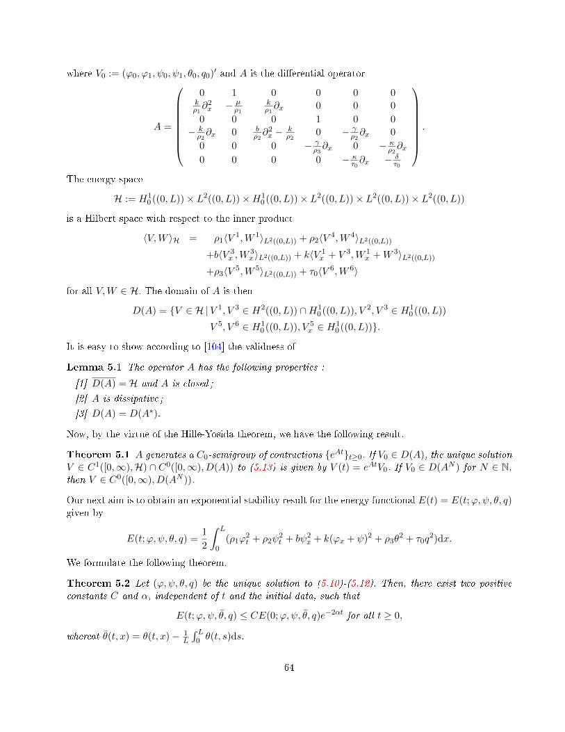
where V0 := (ϕ0, ϕ1, ψ0, ψ1, θ0, q0)′ and A is the dierential operator

A =

0 1 0 0 0 0kρ1∂2x − µ

ρ1

kρ1∂x 0 0 0

0 0 0 1 0 0

− kρ2∂x 0 b

ρ2∂2x − k

ρ20 − γ

ρ2∂x 0

0 0 0 − γρ3∂x 0 − κ

ρ2∂x

0 0 0 0 − κτ0∂x − δ

τ0

.

The energy space

H := H10 ((0, L))× L2((0, L))×H1

0 ((0, L))× L2((0, L))× L2((0, L))× L2((0, L))

is a Hilbert space with respect to the inner product

〈V,W 〉H = ρ1〈V 1,W 1〉L2((0,L)) + ρ2〈V 4,W 4〉L2((0,L))

+b〈V 3x ,W

3x 〉L2((0,L)) + k〈V 1

x + V 3,W 1x +W 3〉L2((0,L))

+ρ3〈V 5,W 5〉L2((0,L)) + τ0〈V 6,W 6〉

for all V,W ∈ H. The domain of A is then

D(A) = V ∈ H |V 1, V 3 ∈ H2((0, L)) ∩H10 ((0, L)), V 2, V 3 ∈ H1

0 ((0, L))

V 5, V 6 ∈ H10 ((0, L)), V 5

x ∈ H10 ((0, L)).

It is easy to show according to [104] the validness of

Lemma 5.1 The operator A has the following properties :

[1] D(A) = H and A is closed ;

[2] A is dissipative ;

[3] D(A) = D(A∗).

Now, by the virtue of the Hille-Yosida theorem, we have the following result.

Theorem 5.1 A generates a C0-semigroup of contractions eAtt≥0. If V0 ∈ D(A), the unique solutionV ∈ C1([0,∞),H) ∩ C0([0,∞), D(A)) to (5.13) is given by V (t) = eAtV0. If V0 ∈ D(AN ) for N ∈ N,then V ∈ C0([0,∞), D(AN )).

Our next aim is to obtain an exponential stability result for the energy functional E(t) = E(t;ϕ,ψ, θ, q)given by

E(t;ϕ,ψ, θ, q) =1

2

∫ L

0(ρ1ϕ

2t + ρ2ψ

2t + bψ2

x + k(ϕx + ψ)2 + ρ3θ2 + τ0q

2)dx.

We formulate the following theorem.

Theorem 5.2 Let (ϕ,ψ, θ, q) be the unique solution to (5.10)-(5.12). Then, there exist two positiveconstants C and α, independent of t and the initial data, such that

E(t;ϕ,ψ, θ, q) ≤ CE(0;ϕ,ψ, θ, q)e−2αt for all t ≥ 0,

whereat θ(t, x) = θ(t, x)− 1L

∫ L0 θ(t, s)ds.

64

5.1.2 Linear exponential stability : ϕx = ψ = q = 0

The second set of boundary conditions we are going to study here is

ϕx(t, 0) = ϕx(t, L) = ψ(t, 0) = ψ(t, L) = q(t, 0) = q(t, L) = 0 in (0,∞). (5.14)

Here, we consider the initial boundary value problem (5.10), (5.12) and (5.14). We will present asemigroup formulation of this problem, show the exponential stability of the associated semigroupand make estimates on higher energies. This will enable us to prove global existence and exponentialstability also in nonlinear settings.Let

L2∗((0, L)) =

u ∈ L2((0, L))

∣∣ ∫ L

0u(x)dx = 0

,

H1∗ ((0, L)) =

u ∈ H1((0, L))

∣∣ ∫ L

0u(x)dx = 0

.

We introduce a Hilbert space

H := H1∗ ((0, L))× L2

∗((0, L))×H10 ((0, L))× L2((0, L))× L2

∗((0, L))× L2((0, L))

equipped with the inner product

〈V,W 〉H = ρ1〈V 1,W 1〉L2((0,L)) + ρ2〈V 4,W 4〉L2((0,L))

+b〈V 3x ,W

3x 〉L2((0,L)) + k〈V 1

x + V 3,W 1x +W 3〉L2((0,L))

+ρ3〈V 5,W 5〉L2((0,L)) + τ0〈V 6,W 6〉.

Let the operator A be formally dened as in section 5.1.1 with the domain

D(A) = V ∈ H |V 1 ∈ H2((0, L)), V 1x ∈ H1

0 ((0, L)), V 2 ∈ H1∗ ((0, L)),

V 3 ∈ H2((0, L)), V 4 ∈ H10 ((0, L)),

V 5 ∈ H1∗ ((0, L)), V 6 ∈ H1

0 ((0, L)).

Setting V := (ϕ,ϕt, ψ, ψt, θ, q)′, we observe that V satises

Vt = AVV (0) = V0

, (5.15)

where V0 := (ϕ0, ϕ1, ψ0, ψ1, θ0, q0)′

By assuring that A satises the conditions of the Hille-Yosida theorem, we can easily get

Theorem 5.3 A generates a C0-semigroup of contractions eAtt≥0. If V0 ∈ D(A), the the uniquesolution V ∈ C1([0,∞),H) ∩ C0([0,∞), D(A)) to (5.15) is given by V (t) = eAtV0. If V0 ∈ D(AN ) forN ∈ N, then V ∈ C0([0,∞), D(AN )).

Observing for the energy E(t) of the unique solution (ϕ,ψ, θ, q) that

E(t) =1

2‖V ‖2H

holds independent of t, we obtain the exponential stability of the associated semigroup eAtt≥0.

65

Theorem 5.4 The semigroup eAtt≥0 associated with A is exponential stable, i.e.

∃c1 > 0 ∀t ≥ 0 ∀V0 ∈ H : ‖eAtV0‖H ≤ c1e−αt‖V0‖H. (5.16)

Similar to [111], we observe that if V0 ∈ D(A), we can estimate AV (t) in the same way as V (t) isestimated in (5.16), implying in its turn using the structure of A that (V 1

x , V2x , V

3x , V

4x , V

5x , V

6x ) can be

estimated in the norm of H, hence, one can estimate ((ϕx)x, (ϕt)x, (ψx)x, (ψt)x, θx, qx)′ in L2((0, L))6.We dene for s ∈ N the Hilbert space

Hs := (Hs ×Hs−1 ×Hs ×Hs−1 ×Hs−1 ×Hs−1)((0, L))

with natural norm Sobolev norm for its component. Using the consideration above, we can thereforeestimate

‖V (t)‖Hs ≤ cs‖V0‖Hse−αt. (5.17)

cs denotes here a positive constant, being independent of V0 and t.

5.1.3 Nonlinear exponential stability

In this subsection, we study the nonlinear system

ρ1ϕtt − σ(ϕx, ψ)x + µϕt = 0,

ρ2ψtt − bψxx + k(ϕx + ψ) + γθx = 0,

ρ3θt + κqx + γψtx = 0, (5.18)

τ0qt + δq + κθx = 0,

in (0,∞)× (0, L), completed by the boundary

ϕ(t, 0) = ϕ(t, L) = ψ(t, 0) = ψ(t, L) = q(t, 0) = q(t, L) = 0 in (0,∞), (5.19)

and the initial conditions

ϕ(0, ·) = ϕ0, ϕt(0, ·) = ϕ1, ψ(0, ·) = ψ0, ψt(0, ·) = ψ1,

θ(0, ·) = θ0, q(0, ·) = q0. (5.20)

As before, the constants ρ1, ρ2, ρ3, b, k, γ, δ, κ, µ, τ0 are assumed to be positive. The nonlinear functionσ is assumed to be suciently smooth and to satisfy

σϕx(0, 0) = σψ(0, 0) = k (5.21)

andσϕxϕx(0, 0) = σϕxψ(0, 0) = σψψ = 0. (5.22)

To obtain a local well-posedness result, we have rst to consider a corresponding non-homogeneouslinear system

ρ1ϕtt − σ(t, x)ϕxx − σ(t, x)ψx + µϕt = 0,

ρ2ψtt − bψxx + k(ϕx + ψ) + γθx = 0,

ρ3θt + κqx + γψtx = 0, (5.23)

τ0qt + δq + κθx = 0,

in (0,∞)× (0, L), together with the boundary conditions (5.19) and initial conditions (5.20).The solvability of this system is established in the following theorem.

66

Theorem 5.5 We assume for some T > 0 that

σ, σ ∈ C1([0, T ]× [0, L]),

σtt, σtx, σxx, σtt, σtx, σxx ∈ L∞([0, T ], L2((0, L))).

Let σ ≥ s > 0. The initial data may satisfy

ϕ0,x ∈ H2((0, L)) ∩H10 ((0, L)), ϕ1,x ∈ H1

0 ((0, L)),

ψ0 ∈ H3((0, L)) ∩H10 ((0, L)), ψ1 ∈ H2((0, L)) ∩H1

0 ((0, L)),

θ0 ∈ H2((0, L)), q0 ∈ H2((0, L)) ∩H10 ((0, L)).

Under the above conditions, the initial boundary problem (5.23), (5.19) and (5.20), possess a uniqueclassical solution (ϕ,ψ, θ, q) such that

ϕ,ψ ∈ C2([0, T ]× [0, L]), θ, q ∈ C1([0, T ]× [0, L]),

∂αϕ, ∂αψ ∈ L∞([0, T ], L2((0, L))), 1 ≤ |α| ≤ 3,

∂αθ, ∂αq ∈ L∞([0, T ], L2((0, L))), 0 ≤ |α| ≤ 2

with ∂α = ∂α1t ∂α2

x for α = (α1, α2) ∈ N20.

Having proved the local linear existence theorem, we can obtain a local existence also in the nonlinearsituation.

Theorem 5.6 Consider the initial boundary value problem (5.18)-(5.20). Let σ = σ(r, s) ∈ C3(R×R)satisfy

0 < r0 ≤ σr ≤ r1 <∞ (r0, r1 > 0), (5.24)

0 ≤ |σs| ≤ s0 <∞ (s0 > 0). (5.25)

Let the initial data comply with

ϕ0,x ∈ H2((0, L)) ∩H10 ((0, L)), ϕ1,x ∈ H1

0 ((0, L)),

ψ0 ∈ H3((0, L)) ∩H10 ((0, L)), ψ1 ∈ H2((0, L)) ∩H1

0 ((0, L)),

θ0 ∈ H2((0, L)), q0 ∈ H2((0, L)) ∩H10 ((0, L)).

The problem (5.18)-(5.20) has then a unique classical solution (ϕ,ψ, θ, q) with

ϕ,ψ ∈ C2([0, T )× [0, L]),

θ, q ∈ C1([0, T )× [0, L]),

dened on a maximal existence interval [0, T ), T ≤ ∞ such that for all t0 ∈ [0, T )

∂αϕ, ∂αψ ∈ L∞([0, t0], L2((0, L))), 1 ≤ |α| ≤ 3,

∂αθ, ∂αq ∈ L∞([0, t0], L2((0, L))), 0 ≤ |α| ≤ 2

holds.

67

To be able to handle the nonlinear problem globally, we need a local existence theorem with higherregularity. This one can be proved in the same way as Theorem 5.6.

Theorem 5.7 Consider the initial boundary value problem (5.18)(5.20). Let σ = σ(r, s) ∈ C4(R×R)satisfy

0 < r0 ≤ σr ≤ r1 <∞ (r0, r1 > 0),

0 ≤ |σs| ≤ s0 <∞ (s0 > 0).

Let the assumptions of Theorem 5.6 be satised. Moreover, let us assume

ϕ0,xxxx, ψ0,xxxx, ϕ1,xxx, ψ1,xxx, θ0,xxx, q0,xxx ∈ L2((0, L))

and

∂2t ϕ(0, ·), ∂2

t ψ(0, ·) ∈ H2((0, L)), ∂2t ϕx(0, ·), ∂2

t ψ(0, ·) ∈ H10 ((0, L))

∂tθ(0, ·), ∂tq(0, ·) ∈ H2((0, L)), ∂tq(0, ·) ∈ H10 ((0, L)).

Then, (5.18)-(5.20) possesses a unique classical solution (ϕ,ψ, θ, q) satisfying

ϕ,ψ ∈ C3([0, T )× [0, L]),

θ, q ∈ C2([0, T )× [0, L]),

being dened in a maximal existence interval [0, T ), T ≤ ∞ such that for all t0 ∈ [0, T )

∂αϕ, ∂αψ ∈ L∞([0, t0], L2((0, L))), 1 ≤ |α| ≤ 4,

∂αθ, ∂αq ∈ L∞([0, t0], L2((0, L))), 0 ≤ |α| ≤ 3

holds. Moreover, this interval coincides with that one from Theorem 5.6.

Remark 5.1 Our conjecture is that in analogy to thermoelastic equations one can prove a more generalexistence theorem by getting bigger regularity of the solution under the same regularity assumptions asin Theorem 5.6 for initial data (cf. [45]).This technique dates back to Kato and is based on a general notion of a CD-system coming from thesemigroup theory.

For the proof of global solvability and exponential stability, we rewrite the problem (5.18)(5.20) intoa nonlinear evolution problem.Letting V = (ϕ,ϕt, ψ, ψt, θ, q) and dening a linear dierential operator A : D(A) ⊂ H → H in thesame manner as in section 5.1.2, we obtain

Vt = AV + F (V, Vx)V (0) = V0

(5.26)

with a nonlinear mapping F being dened by

F (V, Vx) = (0, σϕx(ϕx, ψ)ϕxx − kϕxx + σψ(ϕx, ψ)ψx, 0, 0, 0, 0)′

= (0, σϕx(V 1x , V

3)V 1xx − kV 1

xx + σψ(V 1x , V

3)V 3x − kV 3

x , 0, 0, 0, 0)′.

68

Taking into account that F (V, Vx)(t, ·) ∈ D(A) for V ∈ H3, it follows from the Duhamel's principlethat

V (t) = etAV0 +

∫ t

0e(t−τ)AF (V, Vx)(τ)dr. (5.27)

The existence of a global solution as well as its exponential decay can be proved as in [111] using asimilar technique as for nonlinear Cauchy problems in [103].We assume that the initial data are small in the H2-norm, i.e.

‖V0‖H2 < δ.

Moreover, let us assume the boundness of V0 in the H3-norm, i.e. let

‖V0‖H3 < ν

hold for a ν > 1.Due to the smoothness of the solution, there exist two intervals [0, T 0] and [0, T 1] such that

‖V (t)‖H2 ≤ δ, ∀t ∈ [0, T 0],

‖V (t)‖H3 ≤ ν, ∀t ∈ [0, T 1].

Let d > 1 be a constant to be xed later on. We dene two positive numbers T 1M and T 0

M as the biggestinterval length such that the local solution satises

‖V (t)‖H2 ≤ 2c1δ, ∀t ∈ [0, T 0M ]

and

‖V (t)‖H3 ≤ dν, ∀t ∈ [0, T 1M ],

respectively, fullling ∥∥etAV0

∥∥H2≤ c1‖V ‖H2

for the constant c1 > 0 dened as in (5.17).Under these conditions, we obtain the following estimate for high energy.

Lemma 5.2 There exist positive constants c2, c3 independent of V0 and T such that the local solutionfrom Theorem 5.7 satises for t ∈ [0, T 1

M ] the inequality

‖V (t)‖2H3≤ c2‖V0‖2H3e

c3√dν

∫ t0 ‖V (τ)‖1/2H2

Hτ.

Now, we formulate the theorem on global existence and exponential stability.

Theorem 5.8 Let the assumptions of Theorem 5.7 be fullled. Moreover, let∫ L

0ϕ0(x)dx =

∫ L

0ϕ1(x)dx =

∫ L

0θ(x)dx.

69

Let ν > 1 be arbitrary but xed. We can then nd a δ > 0 such that if ‖V0‖H2 < δ and ‖V1‖H3 < νhold there exists a unique global solution (ϕ,ψ, θ, q) to (5.18)(5.20) satisfying

ϕ,ψ ∈ C3([0,∞)× [0, L]),

θ, q ∈ C2([0,∞)× [0, L]).

There exists besides a constant C0(V0) > 0 such that for all t ≥ 0

‖V (t)‖H2 ≤ C0e−αt

with α > 0 from Theorem 5.4 is valid.

5.2 Timoshenko-type system in thermoelasticity of type III

By the end of the last century, Green and Naghdi [34, 35] introduced three types of thermoelastictheories based on an entropy equality instead of the usual entropy inequality. In each of these theories,the heat ux is given by a dierent constitutive assumption. As a results, three theories are obtainedand were called thermoelasticity types I, type II and type III respectively.This theory is developed in a rational way in order to obtain a fully consistent explanation, which willincorporate thermal pulse transmission in a very logical manner and elevate the unphysical innitespeed of heat propagation induced by the classical theory of heat conduction. When the theory of typeI is linearized the parabolic equation of the heat conduction arises. Whereas the theory of type II donot admit dissipation of energy and it is known as thermoelasticity without dissipation. It is a limitingcase of thermoelasticity type III.In this section, we consider a one-dimensional linear thermoelastic system of Timoshenko type, wherethe heat conduction is given by Green and Naghdi theories. We prove the exponential stability by usingthe energy method.Namely, we consider the following system

ρ1ϕtt −K (ϕx + ψ)x = 0 in (0,∞)× (0, 1) ,ρ2ψtt − bψxx +K (ϕx + ψ) + βθx = 0 in (0,∞)× (0, 1) ,ρ3θtt − δθxx + γψttx − kθtxx = 0 in (0,∞)× (0, 1)ϕ (., 0) = ϕ0, ϕt (., 0) = ϕ1, ψ (t., 0) = ψ0, ψ1 (., 0) = ψ1,θ (., 0) = θ0, θt (., 0) = θ1

ϕ (0, t) = ϕ (1, t) = ψ (0, t) = ψ (1, t) = θ (0, t) = θ (1, t) .

(5.28)

and prove an exponential decay similar to the one in [111]. This system models the transverse vibrationof a thick beam, taking in account the heat conduction given by Green and Naghdi' s theory

5.2.1 Exponential decay

In this subsection, we state and prove our main decay result. In order to exhibit the dissipative natureof system (5.28) we introduce the new variables φ = ϕt and Ψ = ψt. So, problem (5.28) takes the form

ρ1φtt −K (φx + Ψ)x = 0 in (0,∞)× (0, 1)ρ2Ψtt − bΨxx +K (φx + Ψ) + βθtx = 0 in (0,∞)× (0, 1)ρ3θtt − δθxx + γΨtx − kθtxx = 0 in (0,∞)× (0, 1)φ (., 0) = φ0, φt (., 0) = φ1, Ψ (., 0) = Ψ0, Ψt (., 0) = Ψ1

θ (., 0) = θ0, θt (., 0) = θ1

φ (0, t) = φ (1, t) = Ψ (0, t) = Ψ (1, t) = θx (0, t) = θx (1, t) = 0.

(5.29)

70

In order to be able to use Poincaré's inequality for θ, let

θ (x, t) = θ (x, t)− t∫ 1

0θ1 (x) dx−

∫ 1

0θ0 (x) dx .

Then by the third equation in (5.29) we have∫ 1

0θ (x, t) dx = 0, ∀t ≥ 0. (5.30)

In this case, Poincaré's inequality is applicable for θ and on the other hand it is easy to check that(φ,Ψ, θ

)satises the same equations and boundary conditions in (5.29).

Remark 5.2 We can also do this by the same way as in [145] by putting : φ = ϕ,Ψ = ψ, and

Θ(x, t) =

∫ t

0θ (x, s) ds+ χ (x) ,

where χ (x) ∈ H10 (0, 1) solves

χxx = ρ3θ1 − kθ0xx + γψ1x, in (0, 1)χ = 0, x = 0, 1

.

In the sequel we will work with θ but for convenience, we write θ instead of θ. Therefore, the associatedenergy is given by

E (t) =γ

2

∫ 1

0

(ρ1φ

2t + ρ2Ψ2

t +K |φx + Ψ|2 + bΨ2x

)dx+

β

2

∫ 1

0

(ρ3θ

2t + δθ2

x

)dx. (5.31)

Theorem 5.9 Suppose thatρ1

K=ρ2

b(5.32)

andφ0,Ψ0, θ0 ∈ H1

0 (0, 1) , φ1,Ψ1, θ1 ∈ L2 (0, 1) .

Then the energy E (t) decays exponentially as time tends to innity ; that is, there exist two positiveconstants C and ξ independent of the initial data, such that

E (t) ≤ CE (0) e−ξt, ∀t > 0. (5.33)

In [83], we proved Theorem 5.9, by combined several ideas on Timoshenko systems and on thermoelas-ticity of type III. With these combinations, we were able to build an appropriate Lyapunov functionaland proved an exponential decay result.

71

5.3 Timoshenko-type system with history in thermoelasticity of type III

In this section, we consider a one-dimensional linear thermoelastic system of Timoshenko type withpast history acting only in one equation. We consider the model where the heat conduction is givenby Green and Naghdi's theories and prove exponential and polynomial stability results for the equaland non equal wave-speed propagation. Our results are established under conditions on the relaxationfunction weaker than those in [114], in which the authors considered Timoshenko type system withpast history acting only in one equation. More precisely they looked into the following problem

ρ1ϕtt −K(ϕx + ψ)x = 0ρ2ψtt − bψxx +

∫∞0 g(t)ψxx(t− s, .)ds+K(ϕx + ψ) = 0

(5.34)

and showed that the dissipation given by the history term is strong enough to stabilize the systemexponentially if and only if the wave speeds are equal. They also proved that the solution decayspolynomially for the case of dierent wave speeds.In the present work we study the following system

ρ1ϕtt −K (ϕx + ψ)x = 0ρ2ψtt − bψxx +

∫∞0 g (s)ψxx (x, t− s) ds+K (ϕx + ψ) + βθx = 0

ρ3θtt − δθxx + γψttx − kθtxx = 0(5.35)

in (0, 1)× (0,∞), subject to the initial and boundary conditions

ϕ (., 0) = ϕ0, ϕt (., 0) = ϕ1, ψ (t., 0) = ψ0, ψ1 (., 0) = ψ1,

θ (., 0) = θ0, θt (., 0) = θ1 (5.36)

ϕ (0, t) = ϕ (1, t) = ψ (0, t) = ψ (1, t) = θx (0, t) = θx (1, t) = 0 (5.37)

and prove uniform decay results. Precisely, we will show that, forρ1

K=ρ2

b,

the rst energy decays exponentially (resp. polynomially) if g decays exponentially (resp. polynomially).In the case of dierent wave speeds, we show that the decay is of polynomial type. This system modelsthe transverse vibration of a thick beam, taking in account the heat conduction given by Green andNaghdi' s theory.Following the idea of Dafermos [20], we introduce

ηt (x, s) = ψ (x, t)− ψ (x, t− s) , s ≥ 0; (5.38)

consequently we obtain the following initial and boundary conditions

ηt (x, 0) = 0, ∀t ≥ 0 (5.39)

ηt (0, s) = ηt (1, s) = 0, ∀s, t ≥ 0 (5.40)

η0 (x, s) = η0 (s) , ∀s ≥ 0. (5.41)

Clearly, (5.38) givesηtt (x, s) + ηts (x, s) = ψt (x, t) . (5.42)

We also assume that g is a dierentiable function satisfying

g(t) > 0, b = b−∫ ∞

0g (s) ds > 0, g′(t) ≤ −k0g

p(t) (5.43)

for a positive constant k0 and 1 ≤ p < 3/2.

72

Remark 5.3 Under condition (5.43), it is easy to verify that

G0 =

∫ ∞0

g1/2 (s) ds <∞, Gp =

∫ ∞0

g2−p (s) ds <∞, 1 ≤ p < 3/2.

5.3.1 Uniform decay : ρ1

K = ρ2

b

In this subsection, we state and prove our main decay result. In order to exhibit the dissipative natureof system (5.35) we introduce the new variables φ = ϕt , Ψ = ψt, and ηt = ηtt. Thus (5.35)-(5.42) yield

ρ1φtt −K (φx + Ψ)x = 0,

ρ2Ψtt − bΨxx −∫∞

0 g (s) ηtxx (x, s) ds+K (φx + Ψ) + βθtx = 0ρ3θtt − δθxx + γΨtx − kθtxx = 0ηtt + ηts −Ψt = 0

(5.44)

where x ∈ (0, 1) , t ≥ 0 and s ≥ 0. We also obtain the following boundary and initial conditions

φ (., 0) = φ0, φt (., 0) = φ1, Ψ (t., 0) = Ψ0, Ψ1 (., 0) = Ψ1

θ (., 0) = θ0, θt (., 0) = θ1 (5.45)

φ (0, t) = φ (1, t) = Ψ (0, t) = Ψ (1, t) = θx (0, t) = θx (1, t) = 0 (5.46)

ηt (x, 0) = 0, ∀t ≥ 0

ηt (0, s) = ηt (1, s) = 0, ∀s, t ≥ 0 (5.47)

η0 (x, s) = η0 (s) , ∀s ≥ 0.

In order to use the Poincaré inequality for θ, we introduce

θ = θ (x, t)− t∫ 1

0θ1 (x) dx−

∫ 1

0θ0 (x) dx

Then by the third equation in (5.44) we easily verify that∫ 1

0θ (x, t) dx = 0

for all t ≥ 0, in this case the Poincaré inequality is applicable for θ. On the other hand(φ,Ψ, θ, ηt

)satises the same partial dierential equations (5.44) and boundary conditions (5.45)-(5.47). In thesequel we shall work with θ but we write θ for simplicity. Then the associated rst-order energy is

E (t) = = E1(φ,Ψ, θ, ηt) (5.48)

=γ

2

∫ 1

0

(ρ1φ

2t + ρ2Ψ2

t +K |φx + Ψ|2 + bΨ2x

)dx

+β

2

∫ 1

0

(ρ3θ

2t + δθ2

x

)dx+

γ

2

∫ 1

0

∫ ∞0

g (s)∣∣ηtx (s)

∣∣2 dsdx.Our stability result reads as follows.

73

Theorem 5.10 Suppose thatρ1

K=ρ2

b(5.49)

and letφ0,Ψ0, θ0 ∈ H1

0 (0, 1) , ηt0 ∈ L2g

(R+, H1

0 (0, 1)), φ1,Ψ1, θ1 ∈ L2 (0, 1) .

Then there exist two positive constants C and ξ such that

E (t) ≤ Ce−ξt, p = 1 (5.50)

E (t) ≤ C

(t+ 1)1/(p−1)p > 1 (5.51)

5.3.2 Polynomial decay : ρ1

K 6=ρ2

b

In this subsection, we show that in the case of dierent wave-speed propagation (ρ1

K 6=ρ2

b ), the solutionenergy E(t) decays in a polynomial rate even if the relaxation function g decays exponentially providedthat the initial data are regular enough. Let's dene the second-order energy by

E2 (t) = E1(φt,Ψt, θt, ηtt), (5.52)

where E1 is given in (5.48).

Theorem 5.11 Suppose thatρ1

K6= ρ2

b(5.53)

and let

φ0,Ψ0, θ0 ∈ H2 (0, 1) ∩H10 (0, 1) , ηt0 ∈ L2

g

(R+, H2 (0, 1) ∩H1

0 (0, 1)),

φ1,Ψ1, θ1 ∈ H10 (0, 1) . (5.54)

Then there exists a positive constants C, such that

E (t) ≤ C

t1/pp ≥ 1. (5.55)

Remark 5.4 Note that our result is proved without any condition on g′′and g

′′′unlike what was

assumed in [4]. We only need g to be dierentiable and satisfying (5.43).

74

Références

[1] R. A. Adams. Sobolev spaces. Academic Press, New York,, 25, 1975.

[2] K. Agre and M. A. Rammaha. Systems of nonlinear wave equations with damping and sourceterms. Di. Integral Equations, 19(11) :12351270, 2007.

[3] M.R. Alaimia and N. Tatar. Blow up for the wave equation with a fractional damping. J. Appl.Anal., 11(1) :133144, 2005.

[4] F. Amar-Khodja, A. Benabdallah, J. E. Munoz Rivera, and R. Racke. Energy decay for Timo-shenko systems of memory type. J. Di. Equations, 194(1) :82115, 2003.

[5] D. Andrade and L. H. Fatori. The nonlinear transmission problem with memory. Journal ofThermal Stress, 221 :106118, 2004.

[6] D. Andrade, L. H. Fatori, and J. E. Munoz Rivera. Nonlinear transmission problem with adissipative boundary condition of memory type. Electron. J. Di. Equs., 53 :116, 2006.

[7] G. Andrews. On the existence of solutions to the equation utt − uxxt = s(ux)x. J. Di. Eqns.,35 :200231, 1980.

[8] K. T. Andrews, K. L. Kuttler, and M. Shillor. Second order evolution equations with dynamicboundary conditions. J. Math. Anal. Appl., 197(3) :781795, 1996.

[9] D. D. Ang and A. P. N. Dinh. Strong solutionsof quasilinearwave equation with nonlineardamping. SIAM J. Math. Anal., 19 :337347, 1988.

[10] J. Ball. Remarks on blow up and nonexistence theorems for nonlinear evolutions equations.Quart. J. Math. Oxford., 28(2) :473486, 1977.

[11] V. Bayrak and M. Can. Global nonexistence and numerical instabilities of the vibrations of ariser. Math. Comput. Appl., 2(1) :4552, 1997.

[12] J. T. Beale. Spectral properties of an acoustic boundary condition. Indiana Univ. Math. J.,25(9) :895917, 1976.

[13] A. Benaissa and S.A. Messaoudi. Blow up of solutions of a nonlinear wave equation. J. Appl.Math., 2(2) :105108, 2002.

[14] J. Boussinesq. Théorie des ondes et des remous qui se propagent le long d'un canal rectangulairehorizontal, en communiquant au liquide contenu dans ce canal des vitesses sensiblement pareillesde la surface au fond. J. Math. Pure Appl., 38(17) :55 108, 1872.

[15] B. M. Budak, A. A. Samarskii, and A. N. Tikhonov. A collection of problems on mathematicalphysics. Translated by A. R. M. Robson. The Macmillan Co., New York, 1964.

[16] C. Castro and E. Zuazua. Boundary controllability of a hybrid system consisting in two exiblebeams connected by a point mass. SIAM J. Control Optimization, 36(5) :15761595, 1998.

[17] D. S. Chandrasekharaiah. Hyperbolic thermoelasticity : a review of recent literature. Appl. Mech.Rev., 51 :705729, 1998.

[18] S. Chen, K. Liu, and Z. Liu. Spectrum and stability for elastic systems with global or localkelvin-voigt damping. SIAM J. Appl. Math., 59(2) :651668, 1999.

[19] F. Conrad and Ö. Morgül. On the stabilization of a exible beam with a tip mass. SIAM J.Control Optim., 36(6) :19621986 (electronic), 1998.

[20] C. M. Dafermos. Asymptotic stability in viscoelasticity. Arch. Rational Mech. Anal., 37 :297308,1970.

75

[21] R. Dautray and J. L. Lions. Analyse mathématiques et calcul numérique pour les sciences et lestechniques. volume 18, pages 325338. Masson, Paris, 1984.

[22] G.G. Doronin and N. A. Larkin. Global solvability for the quasilinear damped wave equation withnonlinear second-order boundary conditions. Nonlinear Anal., Theory Methods Appl., 8 :11191134, 2002.

[23] J. Esquivel-Avila. Qualitative analysis of a nonlinear wave equation. Discrete. Contin. Dyn.Syst., 10 :787804, 2004.

[24] L. H. Fatori, E. Lueders, and J. E. Munoz Rivera. Transmission problem for hyperbolic ther-moelastic systems. J. Thermal Stresses, 26(7) :739763, 2003.

[25] A. Favini, C. G. Gal, G. Ruiz Goldstein, J.A. Goldstein, and S. Romanelli. The non-autonomouswave equation with general Wentzell boundary conditions. Proc. Roy. Soc. Edinburgh Sect. A,135(2) :317329, 2005.

[26] D-X. Feng, D-H. Shi, and W. Zhang. Boundary feedback stabilization of Timoshenko beam withboundary dissipation. Sci. China. Ser., 41(5) :483490, 1998.

[27] V.A. Galaktinov and S.I. Pohozaev. Blow up and critical exponents for nonlinear hyperbolicequations. Nonlinear Anal., 53 :155182, 2003.

[28] F. Gazzola and M. Squassina. Global solutions and nite time blow up for damped semolinearwave equations. Ann. I. H. Poincaré, 23 :185207, 2006.

[29] V. Georgiev and G. Todorova. Existence of a solution of the wave equation with nonlineardamping and source term. J. Di. Eq., 109 :295308, 1994.

[30] S. Gerbi and B. Said-Houari. Asymptotic stability and blow up a semilinear damped waveequation with dynamic boundary conditions. Submitted.

[31] S. Gerbi and B. Said-Houari. Local existence and exponential growth for a semilinear dampedwave equation with dynamic boundary conditions. Advances in Dierential Equations, 13(11-12) :10511074, 2008.

[32] S. Gerbi and B. Said-Houari. Local existence and exponential growth for a semilinear dampedwave equation with dynamic boundary conditions. Advances in Dierential Equations, 13(11-12) :10511074, 2008.

[33] A. Gmira and M. Guedda. A note on the global nonexistence of solutions to vibrations of a riser.Arab. J. Sci. Eng. Sect. A Sci., 27(2) :197206, 2002.

[34] A. E. Green and P. M. Naghdi. A re-examination of the basic postulates of thermomechanics.Proc. Royal Society London. A., 432 :171194, 1991.

[35] A. E. Green and P. M. Naghdi. On undamped heat waves in an elastic solid. J. Thermal Stresses,15 :253264, 1992.

[36] G. Gripenberg, S. O. Londen, and J. Pruss. On a fractional partial dierential equation withdominating linear part. Math. Meth. Appl. Sci., 20(20) :14271448, 1997.

[37] M. Grobbelaar-Van Dalsen. Uniform stabilization of a one-dimensional hybrid thermo-elasticstructure. Math. Methods Appl. Sci., 26(14) :12231240, 2003.

[38] M. Grobbelaar-Van Dalsen and A. Van Der Merwe. Boundary stabilization for the extensiblebeam with attached load. Math. Models Methods Appl. Sci., 9(3) :379394, 1999.

[39] A. Haraux and Zuazua E. Decay estimates for some semilinear damped hyperbolic problems.Arch. Rational Mech. Anal., 150 :191206, 1988.

76

[40] W. J. Hrusa and S. A. Messaoudi. On formation of singularities on one-dimensional nonlinearthermoelasticity. Arch. Rational Mech. Anal., 111 :135151, 1990.

[41] W. J. Hrusa and M. A. Tarabek. On smooth solutions of the cauchy problem in one-dimensionalnonlinear thermoelasticity. Quart. Appl. Math., 47 :631644, 1989.

[42] W.J. Hrusa and J.A. Nohel. The cauchy problem in one-dimensional nonlinear viscoelasticity. J.Di. Eqs., 59 :388412, 1985.

[43] R. Ikehata. Some remarks on the wave equations with nonlinear damping and source terms.Nonlinear. Anal., 27 :11651175, 1996.

[44] R. Ikehata and T. Suzuki. Stable and unstable sets for evolution equations of parabolic andhyperbolic type. Hiroshima Math. J., 26 :475491, 1996.

[45] S. Jiang and R. Racke. Evolution equations in thermoelasticity. monographs and surveys in pureand applied mathematics. volume 112 of Chapman and Hall. CRC Press : Boca Raton, FL, 2000.

[46] V. K. Kalantarov and O. A. Ladyzhenskaya. The occurence of collapse for quasilinear equationsof parabolic and hyperbolic type. J. Soviet. Math., 10 :5370, 1978.

[47] S. Kawashima and Y. Shibata. Global existence and exponential stability of small solutions tononlinear viscoelasticity. Comm. Math. Physics., 148 :1892008, 1992.

[48] J.U. Kim and Y. Renardy. Boundary control of the Timoshenko beam. SIAM J. Control. Optim.,25(6) :14171429, 1987.

[49] M. Kirane. Blow-up for some equations with semilinear dynamical boundary conditions of para-bolic and hyperbolic type. Hokkaido Math. J., 21(2) :221229, 1992.

[50] M. Kirane and N.E. Tatar. Exponential growth for a fractionally damped wave equation. Zeit.Anal. Anw. (J. Anal. Appl.), 22(1) :167177, 2003.

[51] M. Kopackova. Remarks on bounded solutions of a semilinear dissipative hyperbolic equation.Comment. Math. Univ. Carolin., 30(4) :713719, 1989.

[52] S. Lai and Y. H. Wu. The asymptotic solution of the Cauchy problem for a generalized Boussinesqequation. Discrete and Continuous Dynamical Systems Series B, 3(3) :401408, 2003.

[53] S. Lai and Y. H. Wu. The global solution of an initial boundary value problem for the dampedBoussinesq equation. Comm. Pure. Appl. Anal., 3(2) :319328, 2004.

[54] H. A. Levine, S. R. Park, and J. Serrin. Global existence and global nonexistence of solutions ofthe Cauchy problem for a nonlinearly damped wave equation. J. Math. Anal. Appl., 228(1) :181205, 1998.

[55] H. A. Levine and J. Serrin. Global nonexistence theorems for quasilinear evolution equationswith dissipation. Arch. Rational Mech. Anal., 137(4) :341361, 1997.

[56] H. A. Levine and B. D Sleeman. A note on the non-existence of global solutions of initialboundary value problems for the boussinesq equation utt = 3uxxxx + uxx − 12(u2)xx. J. Math.Anal. Appl., 107 :206210, 1985.

[57] H.A. Levine. Instability and nonexistence of global solutions to nonlinear wave equations of theform. Trans. Amer. Math. Soc., 192 :121, 1974.

[58] H.A. Levine. Some additional remarks on the nonexistence of global solutions to nonlinear waveequations. SIAM J. Math. Anal., 5 :138146, 1974.

[59] F. Li. Global existence and blow-up of solutions for a higher-order Kirchho-type equation withnonlinear dissipation. Appl. Math. Lett., 17 :14091414, 2004.

77

[60] W. Littman and L. Markus. Stabilization of a hybrid system of elasticity by feedback boundarydamping. Ann. Mat. Pura Appl., IV. Ser. , 152 :281330, 1988.

[61] K. Liu and Z. Liu. Exponential decay of energy of the Euler-Bernoulli beam with locally distri-buted Kelvin-Voigt damping. SIAM J. Control Optimization, 36(3) :10861098, 1998.

[62] K. Liu and Z. Liu. Exponential decay of energy of vibrating strings with local viscoelasticity. Z.Angew. Math. Phys., 53(2) :265280, 2002.

[63] W. Liu and G. Williams. The exponential stability of the problem of transmission of the waveequation. Bull. Austral. Math. Soc., 57(2) :305327, 1998.

[64] Z. Liu and S. Zheng. Semigroups Associated with Dissipative Systems. Chapman and Hall. CRCPress : Boca Raton,FL, 1999.

[65] A. Marzocchi, J. E. Munoz Rivera, and M. G. Naso. Asymptotic behavior and exponentialstability for a transmission problem in thermoelasticity. Math. Meth. Appl. Sci., 25 :955980,2002.

[66] A. Marzocchi, J. E. Munoz Rivera, and M. G. Naso. Transmission problem in thermoelasticitywith symmetry. IMA Journal of Appl. Math., 63(1) :2346, 2002.

[67] D. Matignon, J. Audounet, and G. Montseny. Energy decay for wave equations with damping offractional order. Proc. Fourth International Conference on Mathematical and Numerical Aspectsof Wave Propagation Phenomena, INRIA-SIAM, Golden, CO, pages 638640, 1999.

[68] S. Messaoudi and B. Said-Houari. Global non-existence of solutions of a class of wave equationswith non-linear damping and source terms. Math. Methods Appl. Sci., 27 :16871696, 2004.

[69] S. Messaoudi and B. Said-Houari. A global nonexistence result for the nonlinearly dampedmulti-dimensional boussinesq equation. Arab. J. Sci. Eng. Sect. A Sci., 1 :5768, 2006.

[70] S. Messaoudi and B. Said-Houari. A blow-up result for a higher-order nonlinear Kirchho-typehyperbolic equation. Appl. Math. Lett., 20(8) :866871, 2007.

[71] S. A. Messaoudi. On weak solutions of semilinear thermoelastic equations. Rev. MaghrebineMath., 1(1) :3140, 1992.

[72] S. A. Messaoudi. Blow up in a nonlinearly damped wave equation. Mathematische Nachrichten.,231 :17, 2001.

[73] S. A. Messaoudi. A blowup result in a multidimensional semilinear thermoelastic system. Elec-tron. J.Dierential Equations, 30 :19, 2001.

[74] S. A. Messaoudi. Decay of solutions of a nonlinear hyperbolic system describing heat propagationby second sound. Applicable Analysis, 81 :201209, 2002.

[75] S. A. Messaoudi. Local existence and blow up in nonlinear thermoelasticity with second sound.Comm. Partial Dierential Equations., 27(7-8) :16811693, 2002.

[76] S. A. Messaoudi, M. Pokojovy, and B. Said-Houari. Nonlinear damped Timoshenko systems withsecond sound - global existence and exponential stability. Math. Meth. Appl. Sci., 32(5) :505534,2009.

[77] S. A. Messaoudi and B. Said-Houari. A decay result in a system of thermo-elasticity type III.Proceedings of the UAE Math-Day, Nova Publishing Company, New York. To appear.

[78] S. A. Messaoudi and B. Said-Houari. Energy decay in a Timoshenko-type system with historyin thermoelasticity of second sound.

78

[79] S. A. Messaoudi and B. Said-Houari. Exponential stability in nonlinear one-dimensional ther-moelasticity of type III. submitted.

[80] S. A. Messaoudi and B. Said-Houari. Uniform decay in a Timoshenko-type system with pasthistory. Journal of Math. Anal. App. In press.

[81] S. A. Messaoudi and B. Said-Houari. Blowup of solutions with positive energy in nonlinearthermoelasticity with second sound. J. Appl. Math., 3 :201211, 2004.

[82] S. A. Messaoudi and B. Said-Houari. Exponential stability in one-dimensional non-linear ther-moelasticity with second sound. Math. Methods Appl. Sci., 28(2) :205232, 2005.

[83] S. A. Messaoudi and B. Said-Houari. Energy decay in a Timoshenko-type system of thermoelas-ticity of type III. J. Math. Anal. Appl, 348(1) :12251237, 2008.

[84] S. A. Messaoudi and B. Said-Houari. Energy decay in a Timoshenko-type system with historyin thermoelasticity of type III. Advances in Dierential Equations, 14(3-4) :375400, 2009.

[85] S. A. Messaoudi and B. Said-Houari. Energy decay in transmission problem in thermoelasticityof type III. IMA Journal of Applied Mathematics, 74(3) :344360, 2009.

[86] S. A. Messaoudi, B. Said-Houari, and N.E. Tatar. Global existence and asymptotic behavior fora fractional dierential equation. Appl. Math. Comput., 188(2) :19551962, 2007.

[87] M. Milla Miranda and L. A. Medeiros. On the existence of global solutions of a coupled nonlinearklein-gordon equations. Funkcial. Ekvac., 30(1) :147161, 1987.

[88] J.A. Nohel and D.F. Shea. Frequency domain methods for volterra equations. Adv. Math.,22 :278304, 1976.

[89] K. Ono. On global existence, asymptotic stability and blowing up of solutions for some degeneratenonlinear wave equations of Kirchho type. Math. Methods Appl. Sci., 20 :151177, 1997.

[90] K. Ono. On global solutions and blow-up solutions of nonlinear Kirchho string with nonlineardissipation. J. Math. Anal. Appl., 216 :321342, 1997.

[91] H. P. Oquendo. Nonlinear boundary stabilization for a transmission problem in elasticity. Non-linear Anal., 52(4) :13311345, 2003.

[92] H. P. Oquendo. Viscoelastic boundary stabilization for a transmission problem in elasticity. IMAJ. Appl. Math., 68(1) :8397, 2003.

[93] L. E. Payne and D. H. Sattinger. Saddle points and instability of nonlinear hyperbolic equations.Israel. J. Math., 22 :273303, 1975.

[94] M. Pellicer. Large time dynamics of a nonlinear spring-mass-damper model. Nonlin. Anal.,69(1) :31103127, 2008.

[95] M. Pellicer and J. Solà-Morales. Analysis of a viscoelastic spring-mass model. J. Math. Anal.Appl., 294(2) :687698, 2004.

[96] M. Pellicer and J. Solà-Morales. Spectral analysis and limit behaviours in a spring-mass system.Commun. Pure Appl. Anal., 7(3) :563577, 2008.

[97] H. Petzeltova and J. Prüss. Global stability of a fractional partial dierential equation. J. Int.Eqs. Appl., 12(3) :323347, 2000.

[98] I. Podlubny. Fractional Dierential Equations, Mathematics in Sciences and Engineering. vol.198, Academic Press, 1999.

79

[99] R. Quintanilla. Instability and non-existence in the nonlinear theory of thermoelasticity withoutenergy dissipation. Contin. Mech. Thermodyn., 13(2) :121129, 2001.

[100] R. Quintanilla. Structural stability and continuous dependence of solutions of thermoelasticityof type III. Discrete Contin. Dyn. Syst. Ser. B.1, 4 :463470, 2001.

[101] R. Quintanilla. Convergence and structural stability in thermoelasticity. Appl. Math. Comput.,135(2-3) :287300, 2003.

[102] R. Quintanilla and R. Racke. Stability in thermoelasticity of type III. Discrete and ContinuousDynamical Systems B, 3(3) :383400, 2003.

[103] R. Racke. Aspects of mathematics. lectures on nonlinear evolution equations. volume E19 ofInitial Value Problem. Friedrich Vieweg and Sohn : Braunschweig, Wiesbaden, 1992.

[104] R. Racke. Thermoelasticity with second soundexponential stability in linear and non-linear1-d. Math. Methods. Appl. Sci., 25(5) :409441, 2002.

[105] R. Racke. Asymptotic behaviour of solutions in linear 2-or 3-d thermoelasticity with secondsound. Quart. Appl. Math., 61(2) :315328, 2003.

[106] C.A. Raposo, J. Ferreira, M.L. Santos, and N.N.O. Castro. Expoenetial stability for the Timo-shenko system with two weak dampings. Appl. Math. Letters, 18 :535541, 2005.

[107] J. E. Munoz Rivera and H. P. Oquendo. The transmission problem of viscoelastic waves. ActaAppl. Math., 62(1) :121, 2000.

[108] J. E. Munoz Rivera and H. P. Oquendo. The transmission problem for thermoelastic beams.Journal of Thermal Stress, 24(12) :11371158, 2001.

[109] J. E. Munoz Rivera and H. P. Oquendo. Transmission problem for viscoelastic beams. Adv.Math. Sci. Appl., 12(1) :120, 2002.

[110] J. E. Munoz Rivera and H. P. Oquendo. A transmission problem for thermoelastic plates. Q.Appl. Math., 62(2) :273293, 2004.

[111] J. E. Munoz Rivera and R. Racke. Mildly dissipative nonlinear Timoshenko, systems-globalexistence and exponential stability. J. Math. Anal. Appl., 276 :248276, 2002.

[112] J. E. Munoz Rivera and R. Racke. Global stability for damped Timoshenko systems. DiscreteContin. Dyn. Syst., 9(6) :16251639, 2003.

[113] J. E. Munoz Rivera and R. Racke. Timoshenko systems with indenite damping. J. Math. Anal.Appl., 341(2) :10681083, 2008.

[114] J. E. Munoz Rivera and H. D. Fernández Sare. Stability of Timoshenko systems with past history.J. Math. Anal. Appl., 339(1) :482502, 2008.

[115] G. Ruiz Goldstein. Derivation and physical interpretation of general boundary conditions. Adv.Dier. Equ., 11(4) :457480, 2006.

[116] B. Said-Houari. A blow up result with positive initial energy of a class of wave equations withnon-linear damping and source terms. J. Appl. Math., To appear.

[117] B. Said-Houari. Energy decay in thermoelasticity with second sound. Submitted.

[118] B. Said-Houari. Interaction between a dissipative term and a source term in a hyperbolic problem.Master thesis, Annaba University, 2002.

[119] B. Said-Houari. Blow-up of positive initial-energy solutions of system of nonlinear wave equationswith damping and source terms. Dierential and Integral Equations, page To appear, 2009.

80

[120] M. De Lima Santos. Decay rates for solutions of a system of wave equations with memory.Electron. J. Di. Equations, 38 :117, 2002.

[121] H. D. Fernández Sare and R. Racke. On the stability of damped Timoshenko systems - Cattaneoversus Fourier's law. Arch. Rational Mech. Anal., 194(1), 2009.

[122] N. Sauer. Linear evolution equations in two Banach spaces. Proc. Roy. Soc. Edinburgh Sect. A,91(3-4) :287303, 1981/82.

[123] I. Segal. Nonlinear partial dierential equations in quantum eld theory. Proc. Symp. Appl.Math. A.M.S, 17 :210226, 1965.

[124] D-H. Shi and D-X. Feng. Exponential decay of Timoshenko beam with locally distributed feed-back. IMA J. Math. Cont. Inf., 18(3) :395403, 2001.

[125] M. Slemrod. Global existence, uniqueness, and asymptotic stability of classical solutions inone-dimensional thermoelasticity. Arch. Rational Mech. Anal., 76 :97133, 1981.

[126] A. Soufyane. Stabilisation de la poutre de Timoshenko. C. R. Acad. Sci. Paris Sér. I Math.,328(8) :731734, 1999.

[127] A. Soufyane and A. Wehbe. Uniform stabilization for the Timoshenko beam by a locally distri-buted damping. Electron. J. Di. Equations, 29 :114, 2003.

[128] M. A. Tarabek. On the existence of smooth solutions in one-dimensional nonlinear thermoelas-ticity with second sound. Quart. Appl. Math., 50(4) :727742, 1992.

[129] N. Tatar. A wave equation with fractional damping. Zeit. Anal. Anw. (J. Anal. Appl.), 22(3) :110, 2003.

[130] N. Tatar. The decay rate for a fractional dierential equations. J. Math. Anal. Appl., 295 :303314, 2004.

[131] N. Tatar. A blow up result for a fractionally damped wave equation. Nonl. Di. Eqs. Appl.(NoDEA), 12(2) :215226, 2005.

[132] S. W. Taylor. Boundary control of the Timoshenko beam with variable physical characteristics.Resarch Report, Dept. Math. Univ. Auckland, 356, 1998.

[133] S. Timoshenko. On the correction for shear of the dierential equation for transverse vibrationsof prismaticbars. Philisophical. Magazine, 41 :744746, 1921.

[134] G. Todorova. Stable and unstable sets for the Cauchy problem for a nonlinear wave with nonlineardamping and source terms. J. Math. Anal. Appl., 239 :213226, 1999.

[135] G. Todorova and E. Vitillaro. Blow-up for nonlinear dissipative wave equations in Rn. J. Math.Anal. Appl., 303(1) :242257, 2005.

[136] V. V. Varlamov. On the initial boundary value problem for the damped Boussinesq equation.Discrete and Continuous Dynamical Systems, 4(3) :431444, 1998.

[137] V. V. Varlamov. Eigenfunction expansion method and the long-time asymptotics for the dampedBoussinesq equation. Discrete and Continuous Dynamical Systems, 7(4) :675702., 2001.

[138] J.L Vazquez and E . Vitillaro. Heat equation with dynamical boundary conditions of reactivetype. Comm. Partial Dierential Equations, 33(4-6) :561612, 2008.

[139] J.L Vazquez and E . Vitillaro. Wave equation with second-order non-standard dynamical boun-dary conditions. Math. Models Methods Appl. Sci., 18(12) :20192054, 2008.

81

[140] E. Vitillaro. Global existence theorems for a class of evolution equations with dissipation. Arch.Rational Mech. Anal., 149 :155182, 1999.

[141] E. Vitillaro. Global existence for the wave equation with nonlinear boundary damping and sourceterms. J. Dierential Equations, 186(1) :259298, 2002.

[142] E. Vitillaro. A potential well theory for the wave equation with nonlinear source and boundarydamping terms. Glasg. Math. J., 44(3) :375395, 2002.

[143] G-Q. Xu and S-P. Yung. Stabilization of Timoshenko beam by means of pointwise controls.ESAIM, Control Optim. Calc. Var., 9 :579600, 2003.

[144] Z. Yang. Existence and asymptotic behavior of solutions for a class of quasi-linear evolutionequations with non-linear damping and source terms. Math. Meth. Appl. Sci., 25 :795814, 2002.

[145] X. Zhang and E. Zuazua. Decay of solutions of the system of thermoelasticity of type III.Commun. Contemp. Math., 5(1) :2583, 2003.

82