Meeting QoS Requirements in a Dynamically PricedCommercial Cellular Network

by

Melanie Bouroche

A dissertation submitted to

the University of Dublin,

in partial fulfillment of the requirements

for the degree of

Master of Science in Computer Science

Department of Computer Science,

University of Dublin, Trinity College

September, 2003

Declaration

I declare that the work described in this dissertation is, except where otherwise stated, entirely myown work and has not been submitted as an exercise for a degree at this or any other university.

Signature of Author . . . . . . . . . . . . . . . . . . . . . . . . . . . . . . . . . . . . . . . . . . . . . . . . . . . . . . . . . . . . . . . . . . . . . . . . . . . . . .Melanie Bouroche

12 September, 2003

Permission to lend and/or copy

I agree that Trinity College Library may lend or copy this dissertation upon request.

Signature of Author . . . . . . . . . . . . . . . . . . . . . . . . . . . . . . . . . . . . . . . . . . . . . . . . . . . . . . . . . . . . . . . . . . . . . . . . . . . . . .Melanie Bouroche

12 September, 2003

Acknowledgements

I would like to thank Mustapha Bouhtou of France Telecom Research and Development for having

proposed this subject. His help and guidance throughout the course of this project and, in particular,

with the mathematical analysis were greatly appreciated. I would like also to thank my supervisor

Meriel Huggard for her time, enthusiasm and guidance all along the year and for all her productive

criticisms. Many thanks to the NDS class for their help and support throughout the year. Finally,

special thanks to Mathieu Robin for all that he has done.

Abstract

With the current trend towards user mobility and ubiquitous computing, cellular networks are be-coming an evermore important feature of day-to-day life, albeit an unseen one. Mobile networks arecharacterised by a scarcity of resources, particularly bandwidth and frequency spectrum. However,for new multimedia applications, such as video telephony, a large amount of these resources is re-quired and, moreover, these applications demand that specific quality of service guarantees are metby the network at all times.In a cellular network, the traffic is highly variable both temporally and spatially. Therefore, dimen-sioning a network so that it can meet peak-time demand is both uneconomic and inefficient, as mostof the time the network will be under-utilised. This leads to frequent and significant congestion inmobile networks, so that, at a certain time and place, users may find it impossible to start a phonecall, or an ongoing phone call may be interrupted. Some solutions have been proposed to alleviatethe problem of congestion without installing new infrastructure. However, these schemes only im-prove the network performance for some incoming traffic rates, but cannot meet QoS guarantees atpeak-times.Another possible solution to this problem is to attempt to modify the user demand to fit the availableresource. This leads to dynamic pricing: charging users according to the current traffic conditions,hence providing negative or positive incentives to regulate the traffic entering the network. As theyknow the price they will be charged, users can decide whether to make the phone call or not, andthe importance of the call will influence their choice. Hence dynamic pricing leads to a naturalprioritisation of calls, ensuring that only low priority calls are blocked.Dynamic pricing has been applied successfully in several domains, but its application to cellularnetworks is an emerging research area and is particularly challenging due to the mobility of users.This project investigates dynamic pricing in cellular networks from a technical perspective. For thispurpose, detailed network and traffic models are defined based on an investigation of current researchin related areas. These models are implemented in a simulator which is then used to test, refine andimprove existing dynamic pricing schemes for both GSM and GSM/GPRS networks.

Contents

1 Introduction 1

1.1 Context . . . . . . . . . . . . . . . . . . . . . . . . . . . . . . . . . . . . . . . . . . . 1

1.2 Project Goal . . . . . . . . . . . . . . . . . . . . . . . . . . . . . . . . . . . . . . . . 2

1.3 Contribution to Knowledge . . . . . . . . . . . . . . . . . . . . . . . . . . . . . . . . 3

1.4 Dissertation Outline . . . . . . . . . . . . . . . . . . . . . . . . . . . . . . . . . . . . 3

2 State Of the Art 4

2.1 Call Admission Control Schemes . . . . . . . . . . . . . . . . . . . . . . . . . . . . . 4

2.2 Dynamic Pricing in Cellular Networks . . . . . . . . . . . . . . . . . . . . . . . . . . 5

2.2.1 Network Use Maximisation vs. Operator Revenue Optimisation . . . . . . . . 6

2.2.2 A Self-Regulated Dynamic Pricing Algorithm for GSM and GPRS . . . . . . 6

2.2.2.1 Description . . . . . . . . . . . . . . . . . . . . . . . . . . . . . . . . 6

2.2.2.2 Implementation . . . . . . . . . . . . . . . . . . . . . . . . . . . . . 7

2.2.2.3 Demand modelling . . . . . . . . . . . . . . . . . . . . . . . . . . . . 9

2.2.2.4 Pricing . . . . . . . . . . . . . . . . . . . . . . . . . . . . . . . . . . 11

2.2.2.5 Results . . . . . . . . . . . . . . . . . . . . . . . . . . . . . . . . . . 12

2.2.2.6 Further work . . . . . . . . . . . . . . . . . . . . . . . . . . . . . . . 12

2.2.3 Integration of Dynamic Pricing with C.A.C. . . . . . . . . . . . . . . . . . . 13

2.2.3.1 Description . . . . . . . . . . . . . . . . . . . . . . . . . . . . . . . . 13

2.2.3.2 Demand modelling . . . . . . . . . . . . . . . . . . . . . . . . . . . . 14

i

2.2.3.3 Pricing . . . . . . . . . . . . . . . . . . . . . . . . . . . . . . . . . . 14

2.2.3.4 Results . . . . . . . . . . . . . . . . . . . . . . . . . . . . . . . . . . 15

2.2.4 Other Work . . . . . . . . . . . . . . . . . . . . . . . . . . . . . . . . . . . . . 15

2.2.4.1 A Dynamic Pricing Scheme for Connection-oriented Services . . . . 16

2.2.4.2 Models for 3G/4G Network Pricing . . . . . . . . . . . . . . . . . . 16

2.3 Dynamic Pricing in Other Industries . . . . . . . . . . . . . . . . . . . . . . . . . . . 17

2.3.1 General Results on Dynamic Pricing . . . . . . . . . . . . . . . . . . . . . . . 17

2.3.2 Fixed Telephony . . . . . . . . . . . . . . . . . . . . . . . . . . . . . . . . . . 18

2.3.3 Internet and Asynchronous Transfer Mode (ATM) . . . . . . . . . . . . . . . 18

2.3.4 Other Industries . . . . . . . . . . . . . . . . . . . . . . . . . . . . . . . . . . 19

2.4 Conclusions . . . . . . . . . . . . . . . . . . . . . . . . . . . . . . . . . . . . . . . . . 19

3 Network Modelling 21

3.1 Traffic Model . . . . . . . . . . . . . . . . . . . . . . . . . . . . . . . . . . . . . . . . 21

3.1.1 GSM Traffic Model . . . . . . . . . . . . . . . . . . . . . . . . . . . . . . . . . 21

3.1.2 GPRS Traffic Model . . . . . . . . . . . . . . . . . . . . . . . . . . . . . . . . 21

3.2 Call Admission Control . . . . . . . . . . . . . . . . . . . . . . . . . . . . . . . . . . 23

3.3 Network Topology . . . . . . . . . . . . . . . . . . . . . . . . . . . . . . . . . . . . . 23

3.3.1 Hand-off Call Modelling . . . . . . . . . . . . . . . . . . . . . . . . . . . . . . 24

3.3.2 Hand-off Call Generation . . . . . . . . . . . . . . . . . . . . . . . . . . . . . 24

3.4 Conclusion . . . . . . . . . . . . . . . . . . . . . . . . . . . . . . . . . . . . . . . . . 25

4 Mathematical Analysis 28

4.1 Model . . . . . . . . . . . . . . . . . . . . . . . . . . . . . . . . . . . . . . . . . . . . 28

4.2 Traffic Admitted in the System . . . . . . . . . . . . . . . . . . . . . . . . . . . . . . 29

4.3 Revenue . . . . . . . . . . . . . . . . . . . . . . . . . . . . . . . . . . . . . . . . . . . 30

4.3.1 Price . . . . . . . . . . . . . . . . . . . . . . . . . . . . . . . . . . . . . . . . . 30

4.3.2 Revenue . . . . . . . . . . . . . . . . . . . . . . . . . . . . . . . . . . . . . . . 30

ii

4.4 Utility . . . . . . . . . . . . . . . . . . . . . . . . . . . . . . . . . . . . . . . . . . . . 34

4.4.1 Blocking Probability . . . . . . . . . . . . . . . . . . . . . . . . . . . . . . . . 34

4.4.2 Utility of a Single User . . . . . . . . . . . . . . . . . . . . . . . . . . . . . . . 34

4.4.3 Total Utility . . . . . . . . . . . . . . . . . . . . . . . . . . . . . . . . . . . . 36

4.4.3.1 Expression . . . . . . . . . . . . . . . . . . . . . . . . . . . . . . . . 36

4.4.3.2 Variation . . . . . . . . . . . . . . . . . . . . . . . . . . . . . . . . . 37

4.5 Conclusions and Limitation of the Mathematical Analysis . . . . . . . . . . . . . . . 37

5 Simulator Description 40

5.1 Motivations . . . . . . . . . . . . . . . . . . . . . . . . . . . . . . . . . . . . . . . . . 40

5.1.1 Motivations for Using a Simulator . . . . . . . . . . . . . . . . . . . . . . . . 40

5.1.2 Motivations for Writing a new Simulator . . . . . . . . . . . . . . . . . . . . . 41

5.2 Specifications . . . . . . . . . . . . . . . . . . . . . . . . . . . . . . . . . . . . . . . . 41

5.3 Design . . . . . . . . . . . . . . . . . . . . . . . . . . . . . . . . . . . . . . . . . . . . 42

5.3.1 Level of Abstraction . . . . . . . . . . . . . . . . . . . . . . . . . . . . . . . . 42

5.3.2 Different Simulator Types . . . . . . . . . . . . . . . . . . . . . . . . . . . . . 42

5.3.3 Different Types of Events . . . . . . . . . . . . . . . . . . . . . . . . . . . . . 42

5.3.4 Organisation of the Simulator . . . . . . . . . . . . . . . . . . . . . . . . . . . 43

5.4 Technical Aspects . . . . . . . . . . . . . . . . . . . . . . . . . . . . . . . . . . . . . . 44

5.4.1 Generalities . . . . . . . . . . . . . . . . . . . . . . . . . . . . . . . . . . . . . 44

5.4.2 Random Number Generation . . . . . . . . . . . . . . . . . . . . . . . . . . . 44

5.4.3 Arrival Rate Modelling . . . . . . . . . . . . . . . . . . . . . . . . . . . . . . 45

5.5 Validation . . . . . . . . . . . . . . . . . . . . . . . . . . . . . . . . . . . . . . . . . . 45

5.5.1 Tests . . . . . . . . . . . . . . . . . . . . . . . . . . . . . . . . . . . . . . . . . 46

5.5.2 Results Reproduction . . . . . . . . . . . . . . . . . . . . . . . . . . . . . . . 46

5.6 Conclusion . . . . . . . . . . . . . . . . . . . . . . . . . . . . . . . . . . . . . . . . . 46

iii

6 Experiments and Results 47

6.1 Steady State . . . . . . . . . . . . . . . . . . . . . . . . . . . . . . . . . . . . . . . . 47

6.1.1 Experiment . . . . . . . . . . . . . . . . . . . . . . . . . . . . . . . . . . . . . 47

6.1.2 Results . . . . . . . . . . . . . . . . . . . . . . . . . . . . . . . . . . . . . . . 48

6.2 Results Corresponding to the Model Used for the Analytical Analysis . . . . . . . . 49

6.2.1 Experiment . . . . . . . . . . . . . . . . . . . . . . . . . . . . . . . . . . . . . 49

6.2.2 Results . . . . . . . . . . . . . . . . . . . . . . . . . . . . . . . . . . . . . . . 49

6.2.3 Conclusion . . . . . . . . . . . . . . . . . . . . . . . . . . . . . . . . . . . . . 49

6.3 Influence of the Target Rate λ∗n . . . . . . . . . . . . . . . . . . . . . . . . . . . . . . 50

6.3.1 Experiment . . . . . . . . . . . . . . . . . . . . . . . . . . . . . . . . . . . . . 50

6.3.2 Results . . . . . . . . . . . . . . . . . . . . . . . . . . . . . . . . . . . . . . . 50

6.4 Influence of the Hand-off Call Model . . . . . . . . . . . . . . . . . . . . . . . . . . . 52

6.4.1 Experiments . . . . . . . . . . . . . . . . . . . . . . . . . . . . . . . . . . . . 52

6.4.2 Results . . . . . . . . . . . . . . . . . . . . . . . . . . . . . . . . . . . . . . . 52

6.4.3 Conclusion . . . . . . . . . . . . . . . . . . . . . . . . . . . . . . . . . . . . . 52

6.5 Influence of Call Holding Time Model . . . . . . . . . . . . . . . . . . . . . . . . . . 52

6.5.1 Motivations . . . . . . . . . . . . . . . . . . . . . . . . . . . . . . . . . . . . . 52

6.5.2 Experiment . . . . . . . . . . . . . . . . . . . . . . . . . . . . . . . . . . . . . 54

6.5.3 Results . . . . . . . . . . . . . . . . . . . . . . . . . . . . . . . . . . . . . . . 56

6.6 Inclusion of GPRS Traffic . . . . . . . . . . . . . . . . . . . . . . . . . . . . . . . . . 57

6.6.1 Experiments . . . . . . . . . . . . . . . . . . . . . . . . . . . . . . . . . . . . 57

6.6.2 Results . . . . . . . . . . . . . . . . . . . . . . . . . . . . . . . . . . . . . . . 59

6.7 Conclusion . . . . . . . . . . . . . . . . . . . . . . . . . . . . . . . . . . . . . . . . . 60

7 Conclusions 62

7.1 Achievements . . . . . . . . . . . . . . . . . . . . . . . . . . . . . . . . . . . . . . . . 62

7.2 Obstacles Overcome . . . . . . . . . . . . . . . . . . . . . . . . . . . . . . . . . . . . 64

7.3 Future Work . . . . . . . . . . . . . . . . . . . . . . . . . . . . . . . . . . . . . . . . 64

iv

A Complete Class Diagrams 66

Bibliography 69

v

List of Figures

2.1 Fitkov-Norris and Khanifar algorithm . . . . . . . . . . . . . . . . . . . . . . . . . . 7

2.2 Fitkov-Norris and Khanifar GPRS detailed algorithm . . . . . . . . . . . . . . . . . 8

2.3 Hou, Yang and Papavassiliou’s algorithm . . . . . . . . . . . . . . . . . . . . . . . . 14

2.4 Diagrams of experiments CSwR (a), CSwRL (b), PSwR (c) and PSwRL (d) . . . . . 16

3.1 Arrival rate variation during the day . . . . . . . . . . . . . . . . . . . . . . . . . . . 26

3.2 Model of a packet service session . . . . . . . . . . . . . . . . . . . . . . . . . . . . . 26

3.3 Wrap-around network topology . . . . . . . . . . . . . . . . . . . . . . . . . . . . . . 27

4.1 λn(t), The new call arrival function . . . . . . . . . . . . . . . . . . . . . . . . . . . . 29

4.2 λadmit(t), The call admission rate . . . . . . . . . . . . . . . . . . . . . . . . . . . . . 30

4.3 Price variation with lambdaN λn . . . . . . . . . . . . . . . . . . . . . . . . . . . . . 31

4.4 Price variation with time for an arrival rate λn(t) . . . . . . . . . . . . . . . . . . . . 31

4.5 Revenue variations . . . . . . . . . . . . . . . . . . . . . . . . . . . . . . . . . . . . . 33

4.6 Variation of the blocking probability over one day . . . . . . . . . . . . . . . . . . . 35

4.7 Variation in the utility of a single user with the blocking probability . . . . . . . . . 35

4.8 Variations in total utility . . . . . . . . . . . . . . . . . . . . . . . . . . . . . . . . . 38

5.1 Events hierarchy . . . . . . . . . . . . . . . . . . . . . . . . . . . . . . . . . . . . . . 43

5.2 Simulator organisation . . . . . . . . . . . . . . . . . . . . . . . . . . . . . . . . . . . 44

6.1 Steady state results . . . . . . . . . . . . . . . . . . . . . . . . . . . . . . . . . . . . . 48

vi

6.2 Relative variation of utility and revenue with the model used for the mathematical

analysis . . . . . . . . . . . . . . . . . . . . . . . . . . . . . . . . . . . . . . . . . . . 50

6.3 Variation of the total users utility and the total revenue over a day with λ∗n . . . . . 51

6.4 Variations of the new call arrival and admission and the hand-off call arrival rate

during the day with the two models of hand-off calls studied . . . . . . . . . . . . . . 53

6.5 Variations of the total revenue over a day in function of λ∗n with both hand-off models 53

6.6 Variations of the total users utility over a day in function of λ∗n with both hand-off

models . . . . . . . . . . . . . . . . . . . . . . . . . . . . . . . . . . . . . . . . . . . . 54

6.7 Variations of the different call holding time models with the price . . . . . . . . . . . 55

6.8 Variation in the total revenue over a day as a function of λ∗n using the different call

holding time models . . . . . . . . . . . . . . . . . . . . . . . . . . . . . . . . . . . . 56

6.9 Variation in the total users utility over a day as a function of λ∗n using the different

call holding time models . . . . . . . . . . . . . . . . . . . . . . . . . . . . . . . . . . 57

6.10 Variations of the revenue and the total users utility as a function of λ∗n for the call-

holding time model 1 (top), model 2 (centre) and model 3 (bottom) . . . . . . . . . 58

6.11 Comparison of the utility for each of the traffic mixes . . . . . . . . . . . . . . . . . 59

6.12 Comparison of the revenue for each of the traffic mixes . . . . . . . . . . . . . . . . . 60

6.13 Variation of the revenue and the total utility as a function of λ∗n for the three scenarios:

pure GSM (top), pure GPRS (centre), mix GSM/GPRS (bottom) . . . . . . . . . . 61

A.1 Simulator organisation: detailed class diagram . . . . . . . . . . . . . . . . . . . . . 67

A.2 Different types of events: detailed class diagram . . . . . . . . . . . . . . . . . . . . . 68

vii

List of Tables

3.1 Summary of GPRS model . . . . . . . . . . . . . . . . . . . . . . . . . . . . . . . . . 23

viii

Chapter 1

Introduction

1.1 Context

With the current trend towards mobile and ubiquitous computing, cellular networks are becoming

an evermore important feature of day-to-day life, albeit an unseen one. Mobile networks are charac-

terised by a scarcity of resources, particularly bandwidth and frequency spectrum. However, many

new multimedia applications such as video telephony have specific resource requirement and demand

that tight quality of service guarantees are met by the network at all times.

To compound the problem, demand on a cellular network differs significantly between peak and

off-peak times [29]. This means that dimensioning a network so that peak hour demand may be met

is both uneconomic and inefficient, as the network capacity will be under-utilised most of the time.

Moreover, the mobility of users in a cellular network can cause unexpected geographical congestion

due to clustering in unexpected areas. These limitations mean that during times of peak demand,

network operators cannot accept all calls while still meeting their users’ quality of service (QoS)

requirements.

The first possible solution to this problem is to increase the network capacity. Cell splitting and

frequency re-use may be used for this purpose. This results in a higher cell density, hence urban areas

now have far more cells per square kilometre than rural ones, but this is expensive and will increase

the overhead due to hand-off calls. Some other solutions to alleviate the congestion problem that do

not require installation of new infrastructure have been proposed. In GSM/GPRS networks, a degree

of flexibility in the number of available channels per cell may be achieved by moving capacity between

cells (dynamic channel assignment) or by using the overlap between cells and allocating calls to cells

according to the level of traffic in each cell (alternate routing) [14, 27]. The main disadvantages of

1

such dynamic capacity allocation techniques are the increased computational load on the system

and the increase in co-channel interference. In UMTS, an adaptative cell-sizing algorithm has been

suggested as a means of relieving congestion [44]. However, this approach fails when traffic is uniform

i.e. when in a cell cluster, all cells are busy at the same time. In recent years, considerable efforts

have focused on Call Admission Control (CAC). The goal of a CAC scheme is to decide whether

or not to accept a call request. Its purpose is to maximise the utilisation of resources while still

providing the required QoS for all calls.

An alternative approach to the network utilisation problem is to attempt to modify the user demand

to fit the available resource. Mobile network users act “selfishly”: as there is no notion of “commu-

nity”, users have no reason to take into account the existence of other users. Therefore, the only

possible incentive on the demand is the price. Currently, most mobile service providers offer cheaper

off-peak calls as a marketing incentive, in an attempt to utilise spare network capacity. However a

major drawback of this scheme is its lack of flexibility and inability to take into account the actual

network load, by merely increasing the tariff when the operator anticipates high demand. A better

solution is to provide a negative or positive incentive according to current traffic conditions. This

approach leads to dynamic pricing, that is, the price is adjusted dynamically based on prevailing

network conditions. One of the possible implementations is that, users would be told the price per

time unit for a call as they are about to make it. This pricing scheme is designed to regulate the

incoming call rate, as some users will decide not to make a phone call if the price is too high.

As the traffic in cellular networks is highly variable in both space and time, the number of users

willing to make a phone call may be instantaneously very high, thus leading to a very high price.

A certain proportion of connection attempts made during the busy period and suppressed due to

the very high price will never be made again. This may represent lost revenue for the service

provider, however this must be compared with the proportion of calls lost due to call blocking and

call dropping. Users may choose whether to proceed with a call or not and the importance of the call

will influence their decision. Therefore dynamic pricing allows a natural prioritisation of the calls to

occur, ensuring than only low priority calls are lost. This is an improvement on the current system,

where calls are lost indiscriminately [9].

1.2 Project Goal

The goal of the work described below is to investigate dynamic pricing in cellular networks. Dynamic

pricing in cellular networks is an emergent field and only a few studies have been conducted in this

area. Existing work focuses mainly on economical studies of the consequences of dynamic pricing

2

(modelling user reaction to changes in price and QoS) and sometimes technical details may have

been neglected. Furthermore, many aspects of cellular networks have yet to be fully investigated;

this includes the use and design of CAC schemes and the specifications of some protocols. For

example, there is on-going work on the resource assignment for GPRS/GSM networks: how are the

resource shared between GPRS and GSM calls? (see [35] for example). Should a GPRS session be

allocated several channels if required? Should some or all of these channels be released if their is no

channels available for voice calls? [7]. This on-going work on the specification of cellular networks

means that it is particularly difficult to create an accurate model of existing and future cellular

networks.

This work seeks to define a model of existing and emerging networks that is as accurate as possible

by surveying the related literature. This model will be then used to test and enhance existing pricing

policies.

1.3 Contribution to Knowledge

This work presents a model for a GSM/GPRS networks, which includes provision for hand-off calls,

CAC and detailed traffic descriptions. A simplified version of this model has been studied analytically

to explore the behaviour of existing pricing schemes in this environment. This has been studied in

more detail through simulation where several aspects of these networks have been explored. The

contribution of this work is threefold: the definition of a model of existing and emergent cellular

networks, the creation of a simulator which implements this accurate model and, hence, is a powerful

tool for studying pricing policies and the exploration of improvements to existing pricing schemes.

1.4 Dissertation Outline

In the following chapter, recent research work in fields related to cellular networks and, in particular

pricing in cellular networks, is reviewed. The achievements and limitations of each of these studies is

outlined. The network model designed by taken into account existing work, is presented in chapter 3.

In the subsequent chapter, a mathematical analysis of a simplified model of the network and traffic

is detailed and its limitations highlighted. This work clearly demonstrates the need for an accurate

network simulator. The simulator specifically written to explore dynamic pricing is described in

chapter 5. Finally, the experiments carried out using this simulator and the results obtained are

presented in chapter 6.

3

Chapter 2

State Of the Art

In this chapter, we briefly review different Call Admission Control schemes proposed in the litera-

ture, discussing the performance and possible deficiencies of each scheme. To improve congestion

avoidance, dynamic pricing may be introduced alongside Call Admission Control. Dynamic pricing

in cellular networks is an emergent research domain. Relatively few theoretical studies [13, 21, 47]

have been conducted in this area and even fewer empirical studies have been performed. A detailed

review of the existing work on dynamic pricing in cellular network is provided in section 2.2. Dy-

namic pricing has already been studied and implemented in other research domains: we draw on the

conclusions of these studies and try to identify how they may be used to improve work on dynamic

pricing in mobile networks in section 2.3.

2.1 Call Admission Control Schemes

The negative effects of congestion in cellular networks are experienced by mobile users everyday:

when a network is congested, the system cannot admit all calls, hence calls may be refused entry

to the network or interrupted while in progress. It is estimated that, with the development of next

generation networks, congestion will occur more often due to an increase in traffic that is attributed

to an increase in data transmission. To alleviate this problem, different Call Admission Control

(CAC) schemes have been proposed. A Call Admission Control scheme is a provisioning strategy

used to limit the number of calls connected to a network in order to reduce network congestion

and provide a desired Quality Of Service (QoS) to users in the system [21]. These are particularly

difficult to design in the case of cellular systems because of the mobility of users: a user can start a

call in one cell and roam to another cell, while the call is still in progress. In this case the call needs

4

to be handed off to the other cell, and will require the allocation of sufficient bandwidth in the cell it

roams into. Hence a call can either be blocked : a bandwidth request for a new call in a congested cell

is not granted, resulting in the call not being able to start, or dropped : a call is interrupted during

its execution because the user roamed to a cell which doesn’t have sufficient available bandwidth. As

users are more sensitive to call dropping (when a conversation is interrupted) than to call blocking

(when a call cannot be made), most CAC schemes try to give hand-off calls priority over new calls.

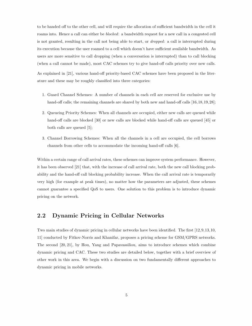
As explained in [21], various hand-off priority-based CAC schemes have been proposed in the liter-

ature and these may be roughly classified into three categories:

1. Guard Channel Schemes: A number of channels in each cell are reserved for exclusive use by

hand-off calls; the remaining channels are shared by both new and hand-off calls [16,18,19,28];

2. Queueing Priority Schemes: When all channels are occupied, either new calls are queued while

hand-off calls are blocked [30] or new calls are blocked while hand-off calls are queued [45] or

both calls are queued [5];

3. Channel Borrowing Schemes: When all the channels in a cell are occupied, the cell borrows

channels from other cells to accommodate the incoming hand-off calls [6].

Within a certain range of call arrival rates, these schemes can improve system performance. However,

it has been observed [21] that, with the increase of call arrival rate, both the new call blocking prob-

ability and the hand-off call blocking probability increase. When the call arrival rate is temporarily

very high (for example at peak times), no matter how the parameters are adjusted, these schemes

cannot guarantee a specified QoS to users. One solution to this problem is to introduce dynamic

pricing on the network.

2.2 Dynamic Pricing in Cellular Networks

Two main studies of dynamic pricing in cellular networks have been identified. The first [12,9,13,10,

11] conducted by Fitkov-Norris and Khanifar, proposes a pricing scheme for GSM/GPRS networks.

The second [20, 21], by Hou, Yang and Papavassiliou, aims to introduce schemes which combine

dynamic pricing and CAC. These two studies are detailed below, together with a brief overview of

other work in this area. We begin with a discussion on two fundamentally different approaches to

dynamic pricing in mobile networks.

5

2.2.1 Network Use Maximisation vs. Operator Revenue Optimisation

There are two fundamentally different approaches to dynamic pricing; the first one explored consid-

ered wireless resources as a public good. In this case, the system aims to ensure that the network

is efficiently used, hence maximising the welfare of the consumers. In term of economics, utility

functions describe users’ level of satisfaction with the perceived quality of service [24], that is, they

characterise how sensitive users are to the changes in QoS. The higher the utility, the more satisfied

the users are. To maximise the use of the network as a public good, the total user utility (the sum of

each individual users utility) should be maximised [24]. This approach leads to users being charged

marginal prices, that is the direct cost of the call to the operator.

A second approach is to maximise network operator revenue. As the network operator sets the

pricing scheme, it is expected that this approach will be more widely used. Furthermore, it has been

estimated that marginal cost pricing does not adequately cover the set up and running costs of the

network operator [25]. Therefore, implementing these charging techniques could lead to reduction of

profitability: the ratio between the amount of capital which is invested into the network (investment)

and the income from it must be such that the basic interest rate on the investment and the expected

profit will be met [48].

It should be noticed than while these are two fundamentally opposing approaches, a third approach

would be to maximise some combination of the total users utility and the operator revenue, hence

leading to a possible compromise between these two goals.

2.2.2 A Self-Regulated Dynamic Pricing Algorithm for GSM and GPRS

2.2.2.1 Description

A simple dynamic pricing algorithm is presented in [12]. The system is self-regulated and its be-

haviour over time is determined by the price charged for each phone call (see figure 2.1). The goal of

this algorithm is to maximise both the revenue for the service operator and the welfare of the users,

that is, to choose the pricing function which offers the best utilisation of system capacity whilst

keeping the call blocking probability at a preset level.

At regular intervals, the system calculates a certain number of operational parameters which de-

termine the network utilisation and performance. These parameters are then compared to a set of

theoretically estimated target values and a decision is reached as to whether a price adjustment needs

to be made. If required, a negative or positive tariff change is calculated, and the price is adjusted

accordingly.

6

Stochastic

Demand Function

S(t)

Deterministic

Demand Function

D(t)

New Price

Calculation

Function p(t)

Is system

optimisation

needed ?

Call Generation Rate

Average call Holding

time

+

Traffic Intensity

Revenue

Grade Of Service

MONITOR YES

NO

Figure 2.1: Fitkov-Norris and Khanifar algorithm

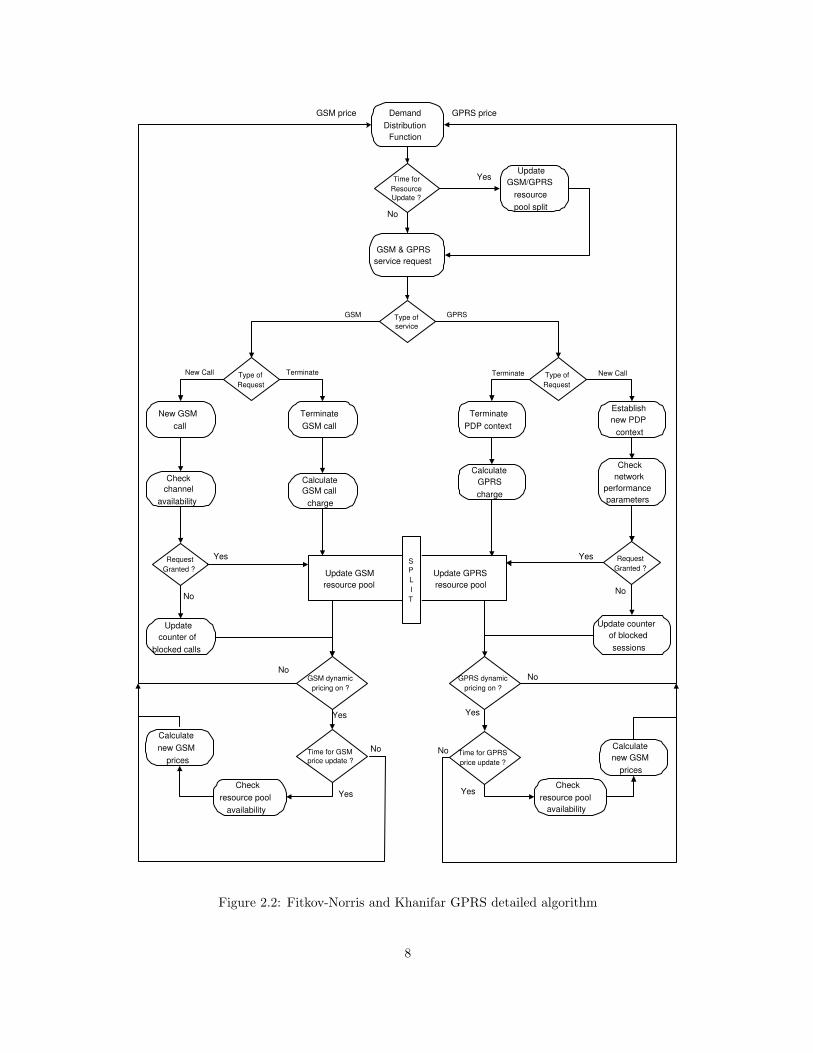
In [11], Fitkov-Norris and Khanifar present a more complex algorithm which provides for the inclusion

of GPRS traffic on the network (c.f. figure 2.2). A function that maps the network load to the price

to be charged is introduced. This is characterised by the divergence, M , of the price curve from

the straight line connecting the minimum and maximum prices. Increasing M will lead to lower

intermediate dynamic prices and reduce the operator revenue, hence M may be interpreted as an

index measuring the welfare of users.

2.2.2.2 Implementation

In the case of GSM networks, Fitkov-Norris and Khanifar propose to implement their algorithm in

the Base Station Controller (BSC). The availability of the necessary data and of spare computational

power make it efficient to compute the price at the BSC; moreover it would minimise the increase

of control traffic in the network.

In UMTS networks, channels cannot be explicitly defined, and it is argued that a possible implemen-

tation of the algorithm would be to charge users on the basis of the interference they cause to other

users. This is known as shadow pricing. In this case, the price charged by the network provider

would be proportional to the total number of users in the network and the amount of bandwidth

used by each user.

7

Demand

Distribution

Function

Time for

Resource

Update ?

Update

GSM/GPRS

resource

pool split

GSM & GPRS

service request

Type of

service

Type of

Request

New GSM

call

Request

Granted ? Update GSM

resource pool

S

P

L

I

T

Update GPRS

resource pool

Type of

Request

Request

Granted ?

GSM dynamic

pricing on ?

Time for GSM

price update ?

GSM price

GPRS dynamic

pricing on ?

Time for GPRS

price update ?

GPRS price

Yes

No

Yes Yes

No

No

No No

Yes Yes

Yes

No No

Yes

GSM GPRS

New Call Terminate New Call Terminate

Terminate

GSM call

Check

channel

availability

Calculate

GSM call

charge

Calculate

GPRS

charge

Terminate

PDP context

Calculate

new GSM

prices

Update

counter of

blocked calls

Check

resource pool

availability

Establish

new PDP

context

Calculate

new GSM

prices

Update counter

of blocked

sessions

Check

network

performance

parameters

Check

resource pool

availability

No

Figure 2.2: Fitkov-Norris and Khanifar GPRS detailed algorithm

8

2.2.2.3 Demand modelling

The user demand is modelled as a combination of a deterministic function D(t), a function of the time

of day which can be predicted fairly accurately, and a random demand S(t) caused, for example, by

emergencies. Depending of the price elasticity of demand, a certain number of calls will be generated.

It is also assumed that the user holding time is inversely proportional to the price charged by the

network.

User Behaviour Model It is expected that mobile network users will change their demand for

network resources in response to tariff changes both in terms of the number of connections requested

and the average call holding time (connection length) [12]. These two, correlated, effects of dynamic

pricing are said to facilitate the convergence of the state of the system to a desired state.

Effect of price on Demand The effect of price on demand is modelled using an exponential

function :

QX = Ae−β.PQX (2.1)

where

– QX is the quantity demanded of good X,

– PQXis the price of good X,

– A is the demand shift constant,

– β is the demand elasticity coefficient.

This model is particularly attractive because the elasticity of the demand can be parameterised and

depends only of the price of the calls [34]. The demand shift constant A will incorporate the change

in demand due to the effect of the time of day using historical data and is therefore time-dependent.

To take existing pricing schemes into account, the model is corrected by taking the difference between

the peak or off-peak price Pbias in the real system and the dynamic price Pdynamic in the modelled

system. Therefore, the basic demand model may be expressed as:

QX = A(t)e−β.(Pbias−Pdynamic) (2.2)

9

Effect of price on User Mobility Fitkov-Norris and Khanifar used the gravity model to repre-

sent the effect of price on user mobility. This model was originally used by Wilson [49], to determine

the most probable distribution of the number of trips between two regions depending on the attrac-

tiveness of the destinations. It has been adapted to predict the number of calls generated between

two cells in a mobile network.

The analogous call gravity model is:

Ψij = κNiNj

(

1

pij

)

(2.3)

where :

– Ψij is the total number of calls between cells i and j,

– κ is a constant,

– pij is the price of the calls between cells i and j,

– Ni is the total number of users in cell i.

To ensure that if the number of users in the cells doubles then the number of calls between the cells

does not quadruple, some corrective constants Ai and Bj are introduced. The resulting model, taking

into account the pricing bias in the historic demand, is, hence, for an exponential cost function:

Ψij = AiBjNiNje−α(pij−pstatic) (2.4)

with

Ai =1

∑

j BjNje−α(pij−pstatic)andBj =

1∑

i AiNie−α(pij−pstatic)

where

– α is an elasticity factor,

– pstatic is the price before introduction of dynamic pricing.

After simplification [13], the model becomes :

Ψij = AiN2i e−α(pij−pstatic) (2.5)

10

with Ai = 1∑

jNje

−α(pij−pstatic) .

Fixed Line Substitution Effect This effect comes into force if the dynamic price of the calls

becomes less than the historic off-peak price. Equation 2.2 becomes:

DQX= A(t)e−β.(Pbias−Pdynamic) + E(Pbias − Pdynamic)

−β (2.6)

2.2.2.4 Pricing

Price Update In [12], operational system parameters such as traffic intensity (Ep), revenue (Rp)

and Grade of Service (GoS) (νp) which determine the network utilisation and performance are

calculated and compared to a set of target system performance parameters which have been estimated

theoretically. A decision is then reached as to whether an adjustment to the tariff is necessary.

The rate of change of the price for the calls determines the degree of demand regulation in the

network [11].

Price Setting In [9,13], two pricing functions, linear and non-linear are examined. In the former

case, the price is linearly proportional to the number of available channels, while in the latter case

the relationship is exponential.

In [11], a more complex pricing function is introduced. This is the solution of the following minimi-

sation problem:

Min

(

∫ Qmax

0

(Pmin + P (q))dq

)

subject to√

1 + P (q)′2dq = M

where

– q is the load of the network

– M is the divergence of the price curve from the straight line connecting the maximum and

minimum price.

The solution is of the form:

P (q) = K − Pmin −√

λ2 − (h − q)2

11

2.2.2.5 Results

This algorithm has been evaluated through simulation [9]. Simulations using both linear and non-

linear pricing functions have been carried out and it has been concluded that dynamic pricing leads

to a significant improvement in the service provider revenue for both types of pricing functions.

However the shape of the pricing function has a significant influence on the total number of blocked

calls in the system. It has been noted that the variation of the generation rate and the resulting

blocked calls in the system are higher for linear pricing functions. The simulation shows an overall

reduction in blocked calls of up to 30%.

2.2.2.6 Further work

In [10], a pricing scheme that maximises the operator revenue is presented. The revenue optimisa-

tion problem may be simplified by dividing the total optimisation period into smaller intervals and

maximising the revenue over each individual interval. The subintervals will be chosen as the length

of time over which the demand time shift constant, A(t), is constant in time. This leads to the

following pricing scheme:

Poptimal =1

β(2.7)

where β is the demand elasticity coefficient of the demand (see section 2.2).

However, this requires a detailed knowledge of the elasticity of the demand (i.e. the aggregate demand

of individual users in the network) and, as such, is not very practical to implement. Furthermore,

with this approach, only the network operator revenue is maximised, without maximising the network

usage (total number of successful calls in the network). It is suggested that a requirement for attaining

a pre-set revenue can be used instead of the maximisation, and in this case the network usage can

be maximised (i.e. it can be ensured that the network is always fully utilised).

An analytical definition of the price which ensures that the capacity is fully utilised without call

blocking, thus offering satisfactory QoS to the users, is given in [10], but in this case the network

operator revenue is not taken into account:

Pdynamic =ln(C + Q( 1−τ

τ)/A(t))

β+ Pbias (2.8)

where:

– C is the capacity of the network,

12

– Q(t) is the instantaneous load,

– τ is the user call holding time,

– A(t) is the demand time shift constant,

– β is the demand elasticity coefficient,

– Pbias is the price already present in the system.

Simulations to compare the two pricing strategies (equations 2.7 and 2.8) have been carried out

and it has been concluded that the revenue generated using the revenue maximisation strategy is

significantly higher than that generated using the existing strategy. Moreover, the revenue generated

using the utilisation maximising strategy is significantly lower than for both the other strategies.

Furthermore, the capacity utilisation pricing strategy is not as effective as the revenue maximisation

strategy in keeping the number of blocked calls down. These results suggest that there is a trade-

off between the effectiveness of dynamic pricing for revenue maximisation and efficient network

utilisation.

2.2.3 Integration of Dynamic Pricing with C.A.C.

The main contribution of Hou, Yang and Papavassiliou is to integrate dynamic pricing with Call

Admissions Control schemes [21,20,19,18].

2.2.3.1 Description

In [20], a wireless network that uses a Guard Channel CAC scheme is considered. The arrival of

new calls is modelled with a Poisson process and the channel holding time is assumed to follow a

negative exponential distribution. Under some further assumptions on the utility function of a single

user, it is proved that there exists an optimal new call arrival rate, λ∗n, which maximises the total

utility of users. Furthermore, for this value the channel resources are most efficiently used. When

the new call arrival rate λn < λ∗n, users can obtain a better QoS than that specified by their QoS

requirements, but some channels resources are wasted. When λn > λ∗n, both the total user utility

and the QoS decrease with any further increase of λn, that is the cell is congested. From the point

of view of guaranteeing QoS , it is preferable for a system to operate with λn < λ∗n.

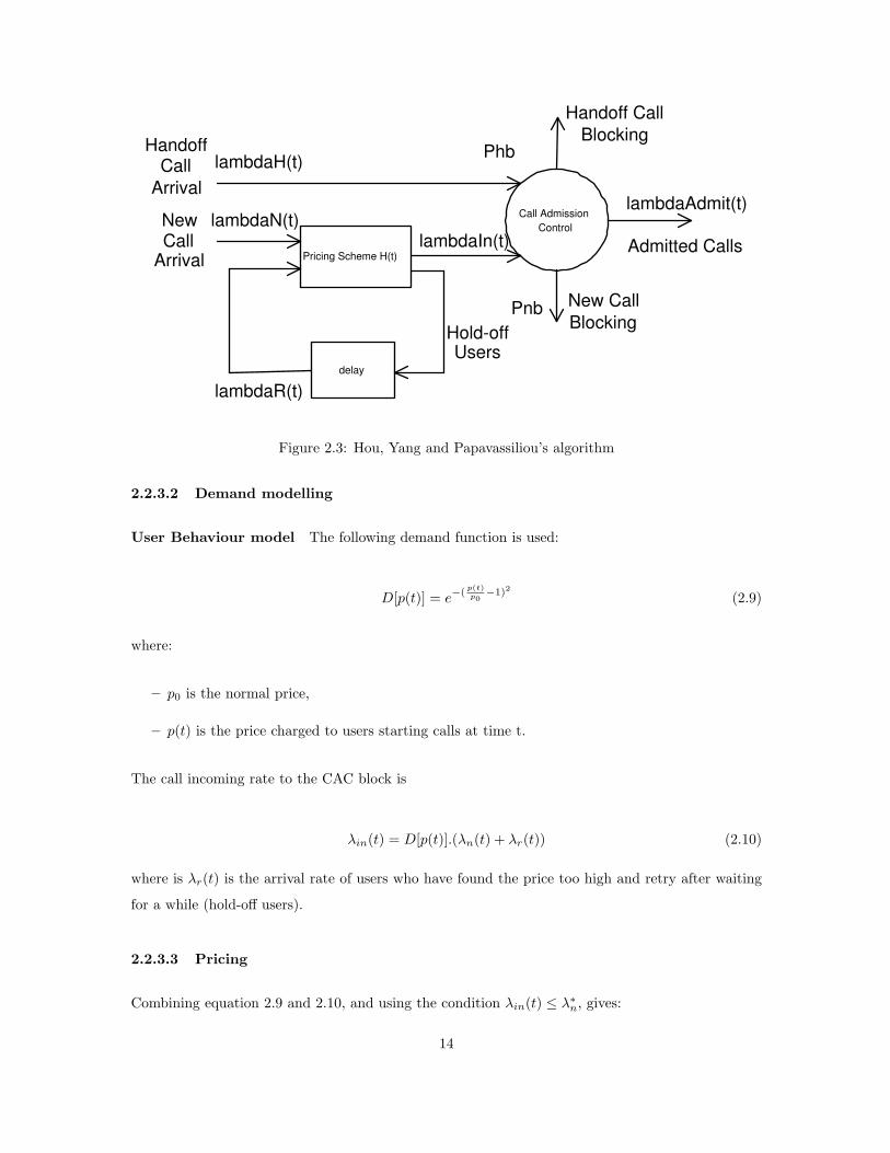
A system composed of two functional blocks, a Pricing block and CAC block, is introduced. When

the traffic load is less that the optimal value, λ∗n, a normal (fixed) price is charged to the user. If

the traffic load increases beyond the optimal value, a dynamic peak hour price depending on current

traffic conditions is charged to users.

13

Call Admission

Control

Pricing Scheme H(t)

delay

Phb

Handoff Call

Blocking

New Call

Blocking

lambdaAdmit(t)

Admitted Calls

Pnb

Handoff Call

Arrival

lambdaH(t)

lambdaN(t) New Call

Arrival lambdaIn(t)

lambdaR(t)

Hold-off Users

Figure 2.3: Hou, Yang and Papavassiliou’s algorithm

2.2.3.2 Demand modelling

User Behaviour model The following demand function is used:

D[p(t)] = e−(p(t)p0

−1)2 (2.9)

where:

– p0 is the normal price,

– p(t) is the price charged to users starting calls at time t.

The call incoming rate to the CAC block is

λin(t) = D[p(t)].(λn(t) + λr(t)) (2.10)

where is λr(t) is the arrival rate of users who have found the price too high and retry after waiting

for a while (hold-off users).

2.2.3.3 Pricing

Combining equation 2.9 and 2.10, and using the condition λin(t) ≤ λ∗n, gives:

14

p(t) = D−1

(

min

(

λ∗n

λn(t) + λr(t), 1

))

(2.11)

This is the price that should be set at time t in order to obtain the desired QoS.

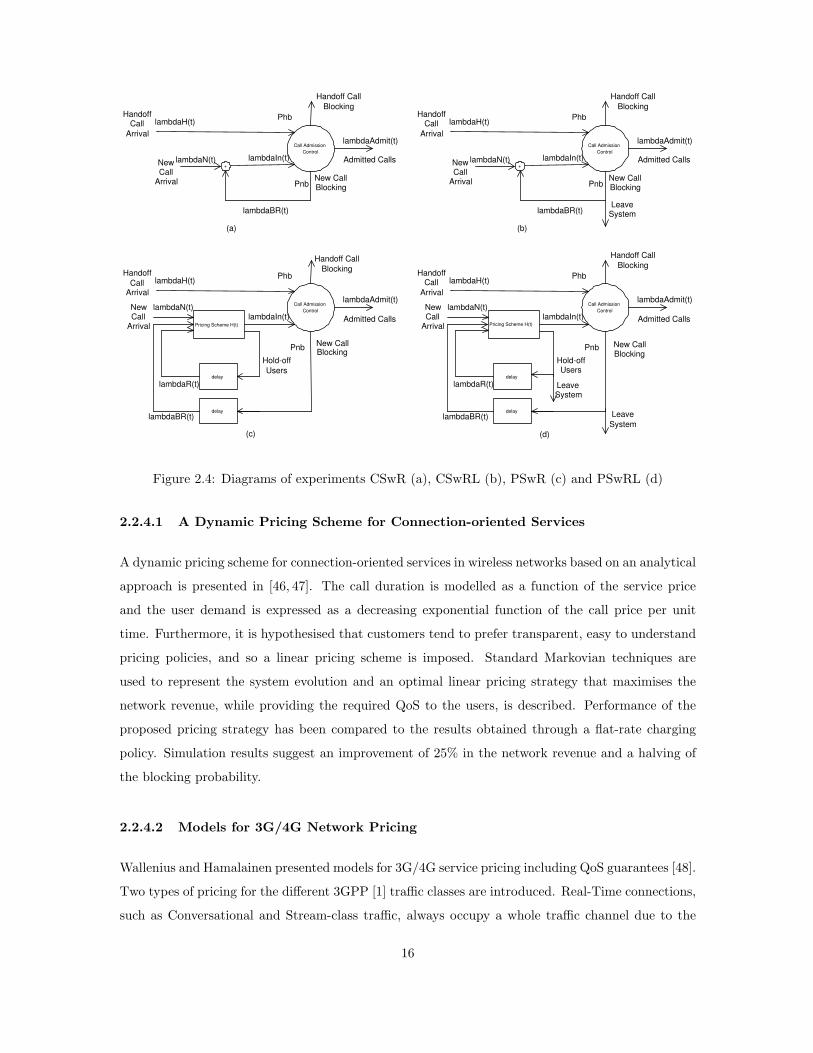
2.2.3.4 Results

The algorithm has been evaluated by simulation [21]. Five experiments were carried out, depending

on the users behaviour (whether after a call being blocked or dropped they retry or not) and on use

of the proposed integrated pricing scheme. The five experiments were as follows:

Conventional System with Retry (CSwR): No pricing block was implemented. Users blocked

by CAC retry after waiting some time.

Conventional System with Retry and Loss (CSwRL): No pricing block was implemented. One

third of the blocked users leaves the system and the rest wait and retry.

Pricing System with Hold-off Retry (PSwHR): The pricing scheme was implemented. A user

that does not accept the current price (hold-off user) waits for some time and retries, while

blocked users leave the system.

Pricing System with Retry (PSwR): Both hold-off and blocked users retry after waiting some

time.

Pricing System with Retry and Loss (PSwRL): One third of the hold-off users and one third

of blocked users leave the system, while other users wait some time and retry.

It was observed that the proposed integrated scheme reduces the occurrence of system congestion and

meets the users’ QoS requirements, while other, conventional, CAC schemes fail to do so. Moreover,

considerable improvements are also observed in both the total user utility achieved and the revenue

obtained.

2.2.4 Other Work

Dynamic pricing in cellular networks has also been considered by Viterbo and Chiasserini [46, 47],

and Wallenius and Hamalainen [48].

15

Call Admission

Control

Phb

Handoff Call

Blocking

New Call Blocking

lambdaAdmit(t)

Admitted Calls

Pnb

Handoff Call

Arrival

lambdaH(t)

lambdaN(t) New Call

Arrival

lambdaIn(t)

lambdaBR(t)

+

(a)

Call Admission

Control

Phb

Handoff Call

Blocking

New Call Blocking

lambdaAdmit(t)

Admitted Calls

Pnb

Handoff Call

Arrival

lambdaH(t)

lambdaN(t) New Call

Arrival

lambdaIn(t)

lambdaBR(t) Leave

System

+

(b)

Call Admission

Control

Pricing Scheme H(t)

delay

Phb

Handoff Call

Blocking

New Call Blocking

lambdaAdmit(t)

Admitted Calls

Pnb

Handoff

Call Arrival

lambdaH(t)

lambdaN(t) New Call

Arrival lambdaIn(t)

delay

lambdaBR(t)

lambdaR(t)

Hold-off

Users

(c)

Call Admission

Control

Pricing Scheme H(t)

delay

Phb

Handoff Call

Blocking

New Call Blocking

lambdaAdmit(t)

Admitted Calls

Pnb

Handoff Call

Arrival

lambdaH(t)

lambdaN(t) New Call

Arrival lambdaIn(t)

delay

lambdaBR(t)

lambdaR(t)

Hold-off Users

Leave System

Leave

System

(d)

Figure 2.4: Diagrams of experiments CSwR (a), CSwRL (b), PSwR (c) and PSwRL (d)

2.2.4.1 A Dynamic Pricing Scheme for Connection-oriented Services

A dynamic pricing scheme for connection-oriented services in wireless networks based on an analytical

approach is presented in [46, 47]. The call duration is modelled as a function of the service price

and the user demand is expressed as a decreasing exponential function of the call price per unit

time. Furthermore, it is hypothesised that customers tend to prefer transparent, easy to understand

pricing policies, and so a linear pricing scheme is imposed. Standard Markovian techniques are

used to represent the system evolution and an optimal linear pricing strategy that maximises the

network revenue, while providing the required QoS to the users, is described. Performance of the

proposed pricing strategy has been compared to the results obtained through a flat-rate charging

policy. Simulation results suggest an improvement of 25% in the network revenue and a halving of

the blocking probability.

2.2.4.2 Models for 3G/4G Network Pricing

Wallenius and Hamalainen presented models for 3G/4G service pricing including QoS guarantees [48].

Two types of pricing for the different 3GPP [1] traffic classes are introduced. Real-Time connections,

such as Conversational and Stream-class traffic, always occupy a whole traffic channel due to the

16

strict delay requirements of the call, and hence can be charged by the duration and the volume of

bits transferred during the call. For non Real-Time Interactive and Background classes, however, a

pricing scheme function of the reserved bandwidth is considered more suitable.

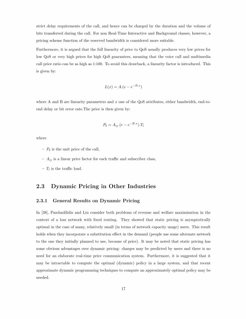
Furthermore, it is argued that the full linearity of price to QoS usually produces very low prices for

low QoS or very high prices for high QoS guarantees, meaning that the voice call and multimedia

call price ratio can be as high as 1:100. To avoid this drawback, a linearity factor is introduced. This

is given by:

L(x) = A.(e − e−B.x)

where A and B are linearity parameters and x one of the QoS attributes, either bandwidth, end-to-

end delay or bit error rate.The price is then given by:

Pb = Aij .(e − e−B.x).Tl

where

– Pb is the unit price of the call,

– Aij is a linear price factor for each traffic and subscriber class,

– Tl is the traffic load.

2.3 Dynamic Pricing in Other Industries

2.3.1 General Results on Dynamic Pricing

In [38], Paschadilidis and Liu consider both problems of revenue and welfare maximisation in the

context of a loss network with fixed routing. They showed that static pricing is asymptotically

optimal in the case of many, relatively small (in terms of network capacity usage) users. This result

holds when they incorporate a substitution effect in the demand (people use some alternate network

to the one they initially planned to use, because of price). It may be noted that static pricing has

some obvious advantages over dynamic pricing: charges may be predicted by users and there is no

need for an elaborate real-time price communication system. Furthermore, it is suggested that it

may be intractable to compute the optimal (dynamic) policy in a large system, and that recent

approximate dynamic programming techniques to compute an approximately optimal policy may be

needed.

17

2.3.2 Fixed Telephony

Some practical pricing experiments have been carried out in students’ dormitories [41]. Shih, Katz

and Joseph conclude that while time-of-the-day pricing encourages users to shift 30% of their usage

from peak to off-peak hours and duration pricing also influences user behaviour; a simple congestion

pricing scheme that charges depending on the number of people calling does not influence call

duration. It is theorised that users do not change their behaviour because they do not know how

long the price increase or decrease will last. Hence it is suggested that, to make a congestion-pricing

scheme more effective, the price changes need to be more permanent to entice users to change their

behaviour. However, it must be noted that, in this experiments carried out, the price per unit of

time varied during the phone call, whereas in most theoretical studies, the price per time unit for a

phone call is set at the beginning of the call. Thus the conclusions reached may not be applicable

for this study.

2.3.3 Internet and Asynchronous Transfer Mode (ATM)

As explained in [39], at present the Internet relies on technical methods to prevent congestion (the

TCP protocol), but includes no mechanism for ensuring QoS guarantees or for delivering service to

those users who need it most. Hence congestion and delay have become a characteristic feature of

the Internet. Pricing mechanisms have the potential to overcome these shortcomings, resulting in

more efficient resource allocation.

There are two possible theoretical approaches to dynamic pricing:

– pricing based on user’s bidding for the available bandwidth,

– pricing based on the amount of congestion caused by the users’ packets.

The first approach, called “smart market”, was developed by MacKie-Mason and Varian [33]: in this

case, the network users bid for the available bandwidth and the network serves the highest bidders

first. A particular problem with this approach is that it can lead to a backlog of lower bid packets. In

addition, the signalling information necessary to complete the bidding may overwhelm the signalling

capacity of the cellular networks.

The second approach is based on retrospective “shadow” pricing depending on the amount of con-

gestion caused by the user [26]. This is achieved by marking packets that cause buffers to overflow.

In the case of ATM, a particular problem with this approach is that the self-similarity of the traffic

makes it difficult to determine when a particular burst of packets ends and when the next one begins

18

so that marking may be stopped. Also, the fact that this pricing scheme is retrospective means that

the user cannot know the price that will be charged in advance.

2.3.4 Other Industries

Real-time (dynamic) pricing has been successfully applied to electricity supplies for both industrial

and residential customers [3, 15, 40, 50, 8]. In general, the response of industrial and residential

customers to real-time pricing was variable and complex but led to reduced bills for the majority of

users.

Another field from which conclusions can be drawn by analogy is financial markets. The prices of

shares are governed by the laws of supply and demand and change dynamically over time. Predictions

for the behaviour of telecommunication networks with dynamic pricing can be made by analogy with

the behaviour of the financial markets. In both cases, the choices that consumers make are dependent

on price as well as additional (chaotic or random) factors.

In the case of revenue maximisation, the problem is essentially a problem of yield management, similar

to the problems that arise in the airline and other service industries [43, 42]. The common problem

in this case is that the marginal cost of serving an additional customer, e.g. an airline passenger

or a new call, is negligible once a flight has been scheduled or a communication infrastructure is in

place [39]. However in cellular network the problem is technically slightly different: the operator

considers a long-term average whereas in airline industry a finite horizon is set (the departure of the

plane) [38].

2.4 Conclusions

For establishing the network pricing policy, two fundamentally opposed approaches can be used

as described in section 2.2.1, but the most realistic and interesting approach is to find a trade-off

between the network utilisation and the provider revenue.

The most complete, and detailed, study of dynamic pricing in cellular networks has been carried out

by Hou, Yang and Papavassiliou (c.f. section 2.2.3). In this work, it was established that there exists

an optimal constant arrival rate to the system for optimising the total user utility, and a pricing

scheme was designed to make the arrival traffic rate fit the optimal one. The optimal arrival rate

was calculated for a steady state, whereas in the real system the regulation of the demand by the

price cannot be perfect. Hence, as the arrival of traffic into the pricing scheme will vary during the

day, the arrival rate into the system will vary also. For this reason, the optimal arrival rate for the

19

real system may be different than the optimal arrival rate for the steady state, as some variation

around it must be taken into account. Because regulation of the traffic by the pricing scheme is not

immediate, signalling that the network is congested before this actually occurs could improve the

total utility of the users by limiting the number of blocked calls. The operator revenue could also

be increased if peak-prices start being charged before the network is congested. On the other hand,

starting to charge peak-prices too early might lead to a reduction of profit due to a decrease in the

number of users in the network.

For these reasons, it seems particularly interesting to make the “optimal” value used in this pricing

scheme vary from the steady state result and to see how the total utility and revenue over a day is

affected. This is one of the main goals of this work. In the following chapter, an analytic study of

the the total utility and the revenue over a day is performed.

20

Chapter 3

Network Modelling

This chapter presents the models used to represent the network and to generate network traffic. Two

types of traffic are generated: GSM and GPRS traffic. The models used for these are now described

in details.

3.1 Traffic Model

3.1.1 GSM Traffic Model

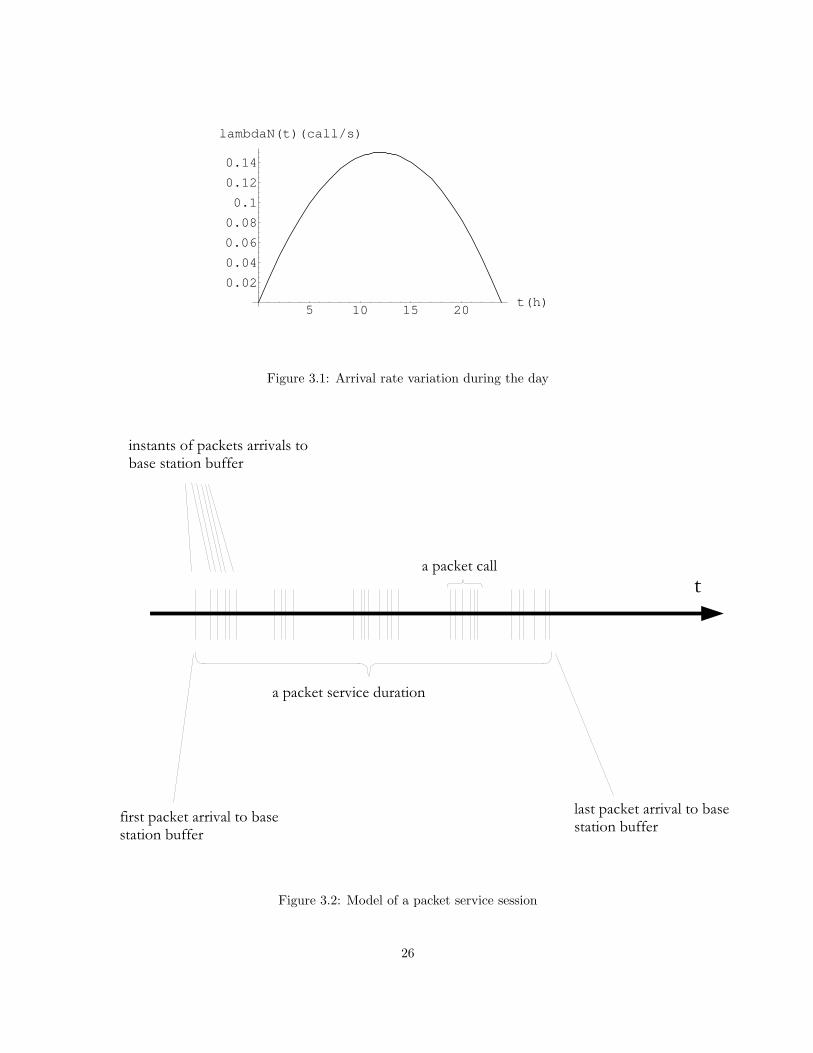
A Poisson process is used to generate the arrival of GSM calls. The call arrival rate varies depending

on the time of the day (see Figure 3.1). The GSM call holding time (total call duration) and cell

dwell time (time a mobile host stays in a cell) are modelled using a geometrical distribution. They

are assumed to be independent of both price and time. When a call is generated, both its call holding

time and cell dwell time are generated and the minimum of these two is used to determine a suitable

event trigger to associate with the call.

3.1.2 GPRS Traffic Model

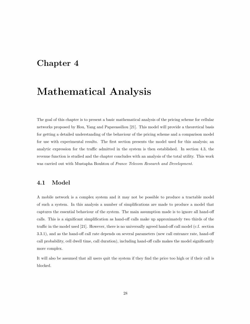
GPRS traffic is generated according to the IETF web traffic model proposed in [22]. It is a unidi-

rectional model: it represents the packets from a source, which may be at either end of the link,

and ignores the uplink traffic. According to this model a web browsing session consists of packet

calls (see Figure 3.2) . Each time a user requires an information entity, a packet call is generated.

A packet call is composed of a certain number of packets, hence it constitutes a bursty sequence of

packets, a characteristic of packet transmission in a fixed network.

21

A packet service session contains one or several packet calls depending on the application. For

example in a web browsing session, a packet call corresponds to the downloading of a web document.

After the document has been successfully downloaded to the terminal, the user takes a certain

amount of time to study the information it contains. This time interval is called the reading time.

It is also possible that the session contains only one packet call; for example for a file transfer, in

this case the session includes no reading time.

The model is made of the following components:

Session Arrival Process: The session arrival in the system is modelled as a Poisson process.

Number of packets calls request by session: This is a geometrically distributed random vari-

able with a mean of 5 packets per session.

Reading time between packet calls: The reading time between two consecutive packet call re-

quests in a session is a geometrically distributed random variable with a mean of 412 seconds.

The reading time starts when the last packet of the packet call is completely received by the

user. It ends when the user makes a request for the next packet call.

Number of packets in a packet call: According to the IETF traffic model, this parameter should

vary depending on the characteristics of UMTS traffic. It is suggested that a geometrically

distributed random variable with a mean of 25 packets is suitable, and this is used in this

simulator.

Time interval between packets: The time interval between two consecutive packets inside a

packet call is a geometrically distributed random variable with a mean which depends of the

average bit rate at the source level. The traffic generator implemented simulates a source with

an average bit rate of 64 kb/s; in this case the mean value of the time interval between two

consecutive packets in a packet call is 62.5 ms.

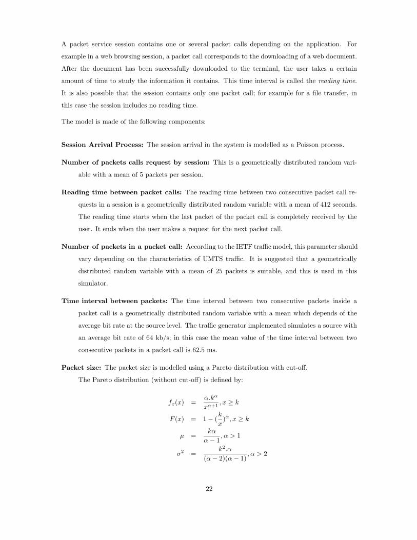
Packet size: The packet size is modelled using a Pareto distribution with cut-off.

The Pareto distribution (without cut-off) is defined by:

fx(x) =α.kα

xα+1, x ≥ k

F (x) = 1 − (k

x)α, x ≥ k

µ =kα

α − 1, α > 1

σ2 =k2.α

(α − 2)(α − 1), α > 2

22

A cut-off of m= 66666 bytes is used and the packet size is defined by :

PacketSize = min(P,m)

where P is a normal Pareto distributed random variable with parameters α = 1.1 and k = 81.5

bytes.

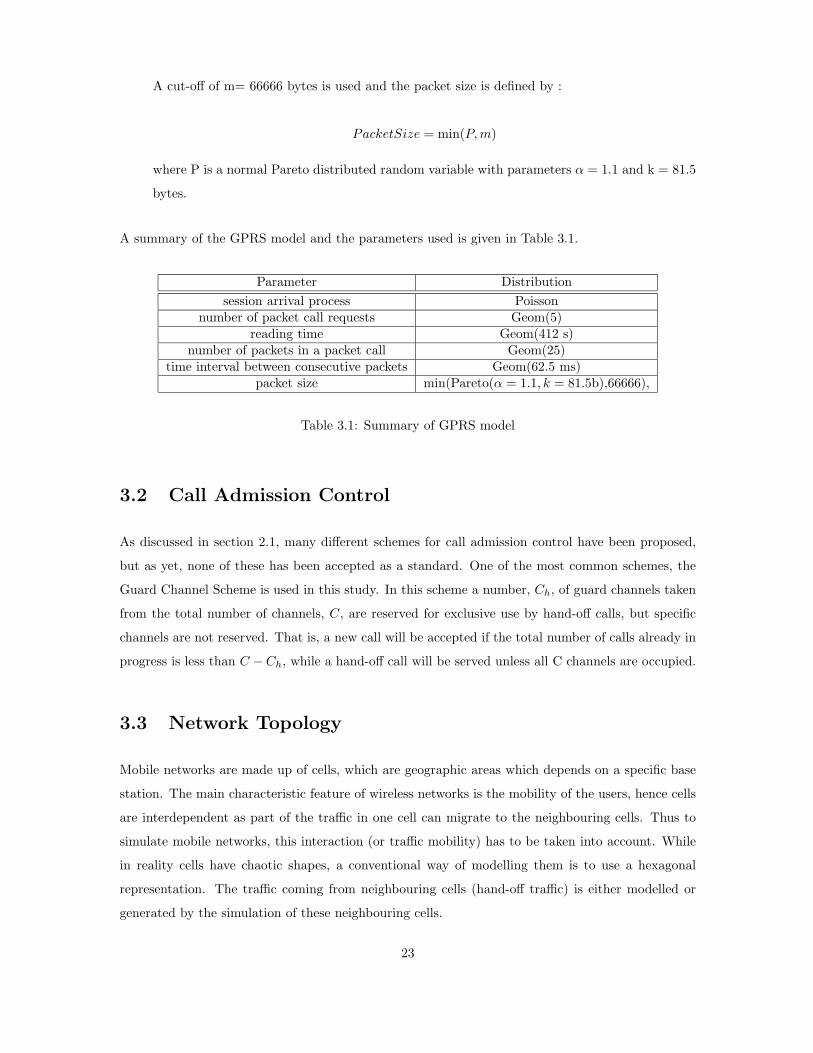
A summary of the GPRS model and the parameters used is given in Table 3.1.

Parameter Distribution

session arrival process Poissonnumber of packet call requests Geom(5)

reading time Geom(412 s)number of packets in a packet call Geom(25)

time interval between consecutive packets Geom(62.5 ms)packet size min(Pareto(α = 1.1, k = 81.5b),66666),

Table 3.1: Summary of GPRS model

3.2 Call Admission Control

As discussed in section 2.1, many different schemes for call admission control have been proposed,

but as yet, none of these has been accepted as a standard. One of the most common schemes, the

Guard Channel Scheme is used in this study. In this scheme a number, Ch, of guard channels taken

from the total number of channels, C, are reserved for exclusive use by hand-off calls, but specific

channels are not reserved. That is, a new call will be accepted if the total number of calls already in

progress is less than C −Ch, while a hand-off call will be served unless all C channels are occupied.

3.3 Network Topology

Mobile networks are made up of cells, which are geographic areas which depends on a specific base

station. The main characteristic feature of wireless networks is the mobility of the users, hence cells

are interdependent as part of the traffic in one cell can migrate to the neighbouring cells. Thus to

simulate mobile networks, this interaction (or traffic mobility) has to be taken into account. While

in reality cells have chaotic shapes, a conventional way of modelling them is to use a hexagonal

representation. The traffic coming from neighbouring cells (hand-off traffic) is either modelled or

generated by the simulation of these neighbouring cells.

23

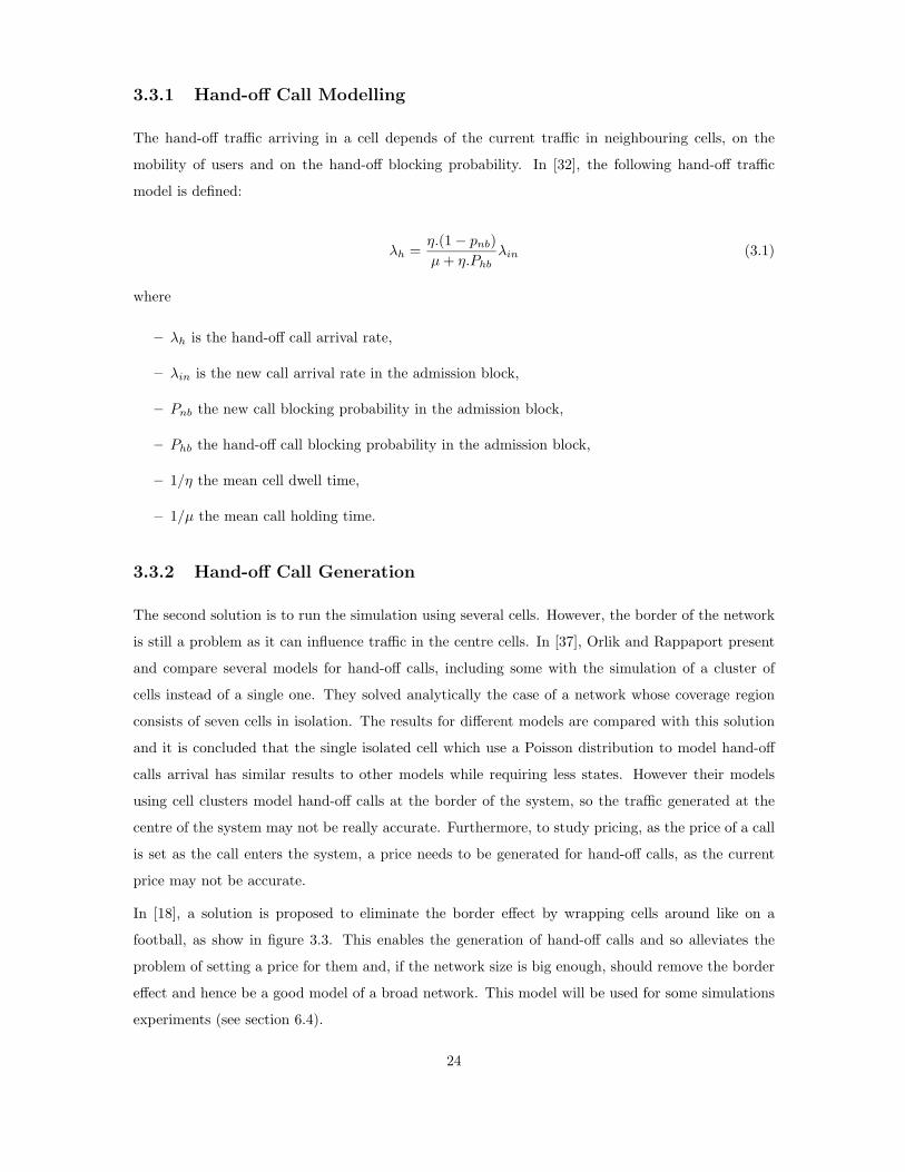
3.3.1 Hand-off Call Modelling

The hand-off traffic arriving in a cell depends of the current traffic in neighbouring cells, on the

mobility of users and on the hand-off blocking probability. In [32], the following hand-off traffic

model is defined:

λh =η.(1 − pnb)

µ + η.Phb

λin (3.1)

where

– λh is the hand-off call arrival rate,

– λin is the new call arrival rate in the admission block,

– Pnb the new call blocking probability in the admission block,

– Phb the hand-off call blocking probability in the admission block,

– 1/η the mean cell dwell time,

– 1/µ the mean call holding time.

3.3.2 Hand-off Call Generation

The second solution is to run the simulation using several cells. However, the border of the network

is still a problem as it can influence traffic in the centre cells. In [37], Orlik and Rappaport present

and compare several models for hand-off calls, including some with the simulation of a cluster of

cells instead of a single one. They solved analytically the case of a network whose coverage region

consists of seven cells in isolation. The results for different models are compared with this solution

and it is concluded that the single isolated cell which use a Poisson distribution to model hand-off

calls arrival has similar results to other models while requiring less states. However their models

using cell clusters model hand-off calls at the border of the system, so the traffic generated at the

centre of the system may not be really accurate. Furthermore, to study pricing, as the price of a call

is set as the call enters the system, a price needs to be generated for hand-off calls, as the current

price may not be accurate.

In [18], a solution is proposed to eliminate the border effect by wrapping cells around like on a

football, as show in figure 3.3. This enables the generation of hand-off calls and so alleviates the

problem of setting a price for them and, if the network size is big enough, should remove the border

effect and hence be a good model of a broad network. This model will be used for some simulations

experiments (see section 6.4).

24

3.4 Conclusion

In this chapter, a model for cellular networks has been presented, alongside with a traffic model. In

the following chapter, a mathematical analysis is carried out on a simplified version of this model.

25

5 10 15 20t(h)

0.02

0.04

0.06

0.08

0.1

0.12

0.14

lambdaN(t)(call/s)

Figure 3.1: Arrival rate variation during the day

Figure 3.2: Model of a packet service session

26

Figure 3.3: Wrap-around network topology

27

Chapter 4

Mathematical Analysis

The goal of this chapter is to present a basic mathematical analysis of the pricing scheme for cellular

networks proposed by Hou, Yang and Papavassiliou [21]. This model will provide a theoretical basis

for getting a detailed understanding of the behaviour of the pricing scheme and a comparison model

for use with experimental results. The first section presents the model used for this analysis; an

analytic expression for the traffic admitted in the system is then established. In section 4.3, the

revenue function is studied and the chapter concludes with an analysis of the total utility. This work

was carried out with Mustapha Bouhtou of France Telecom Research and Development.

4.1 Model

A mobile network is a complex system and it may not be possible to produce a tractable model

of such a system. In this analysis a number of simplifications are made to produce a model that

captures the essential behaviour of the system. The main assumption made is to ignore all hand-off

calls. This is a significant simplification as hand-off calls make up approximately two thirds of the

traffic in the model used [21]. However, there is no universally agreed hand-off call model (c.f. section

3.3.1), and as the hand-off call rate depends on several parameters (new call entrance rate, hand-off

call probability, cell dwell time, call duration), including hand-off calls makes the model significantly

more complex.

It will also be assumed that all users quit the system if they find the price too high or if their call is

blocked.

28

4.2 Traffic Admitted in the System

The same call variational arrival rate model as described in [21] will be used. In this model, the

traffic generation rate follows a parabolic function λn(t) during the day, as in figure 4.1. However,

5 10 15 20t(h)

0.02

0.04

0.06

0.08

0.1

0.12

0.14

lambdaN(t)(call/s)

Figure 4.1: λn(t), The new call arrival function

the specific shape of the new call arrival rate function does not play any part in this analysis; it is

only used to obtain a graphical understanding of the problem. Assuming than the pricing scheme

chosen regulates the traffic perfectly, the traffic entering the system is:

λin(t) = min (λn(t), λ∗n) (4.1)

where λ∗n is the target rate, i.e. the rate the pricing scheme aims to produce at the entrance of the

system.

If we assume that all calls are of equal length, τ , the maximum admission rate to the system in

steady state is λcap = C/τ where C is the network capacity. As the arrival rate varies slowly in

comparison to the life-time of a call τ , we will model the state of the system as a succession of

steady states. Under this assumption, the call admission control block will accept calls at a rate

λadmit(t) = min (λin(t), λcap). The complete expression for the admission rate in the system is:

λadmit(t) = min (λn(t), λ∗n, λcap) (4.2)

Figure 4.2 shows the variation of λadmit(t) over time. The maximal value corresponds to min (λ∗n, λcap).

29

5 10 15 20t(h)

0.02

0.04

0.06

0.08

0.1

0.12

0.14

lambdaAdmit(t) (call/s)

Figure 4.2: λadmit(t), The call admission rate

4.3 Revenue

The variation of the network operator revenue as a function of λ∗n is considered. To do this, the

pricing scheme must be defined.

4.3.1 Price

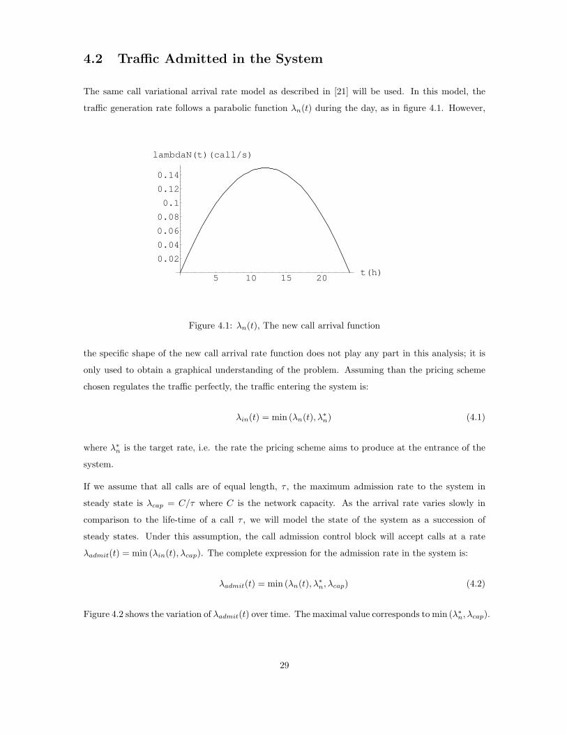
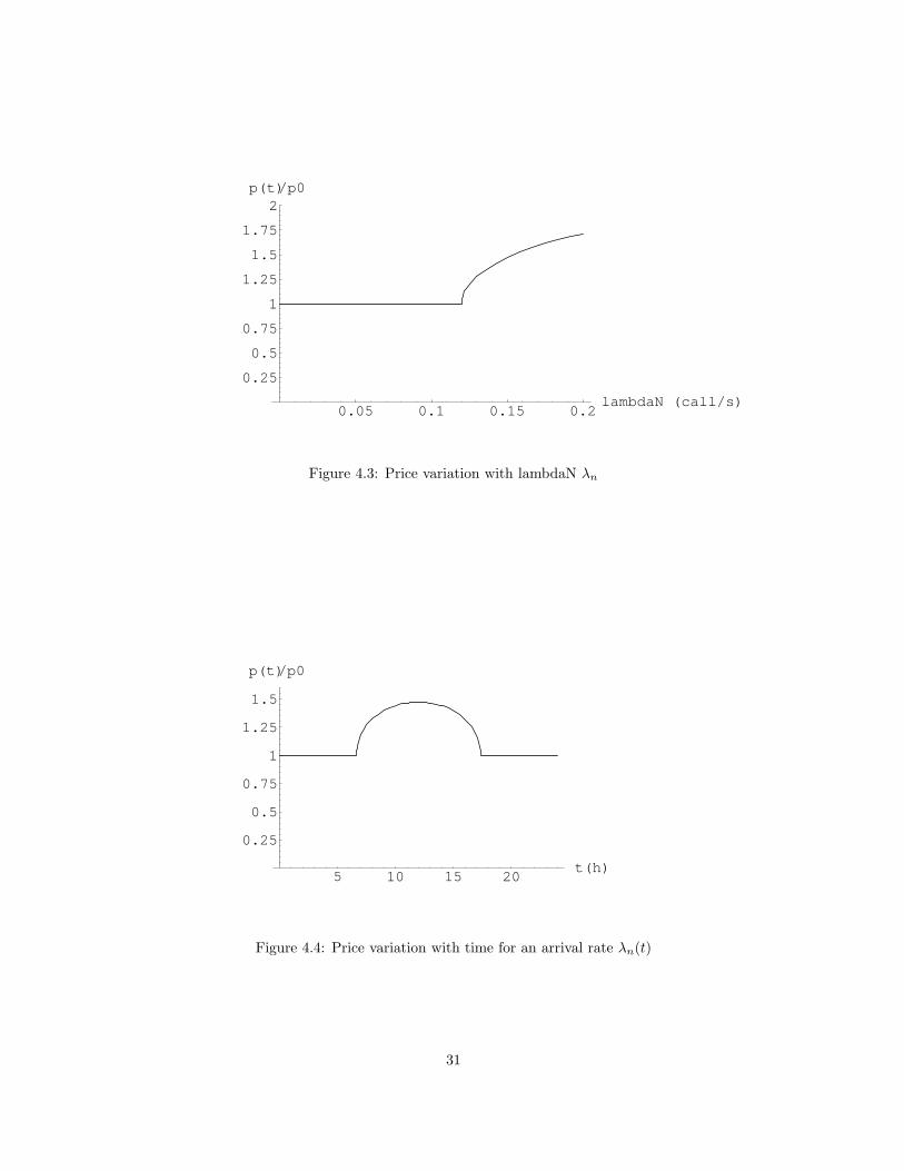
The pricing scheme defined in [21] by Hou, Yang and Papavassiliou is used:

p(t) =

p0 when λn(t) ≤ λ∗n

p0

(

1 +

√

ln(

λn(t)λ∗

n

)

)

when λn(t) ≥ λ∗n

The variation of this pricing scheme as a function of λn and as a function of the time of the day with

an arrival rate λn(t) as defined in the previous section, are shown in figures 4.3 and 4.4 respectively.

4.3.2 Revenue

The expression for the revenue depends of the relative values of λ∗n and λcap; we will consider both

cases:

– For λ∗n < λcap, the network is never actually congested, hence λadmit(t) = min (λn(t), λ∗

n). In

30

0.05 0.1 0.15 0.2lambdaN (call/s)

0.25

0.5

0.75

1

1.25

1.5

1.75

2p(t)/p0

Figure 4.3: Price variation with lambdaN λn

5 10 15 20t(h)

0.25

0.5

0.75

1

1.25

1.5

p(t)/p0

Figure 4.4: Price variation with time for an arrival rate λn(t)

31

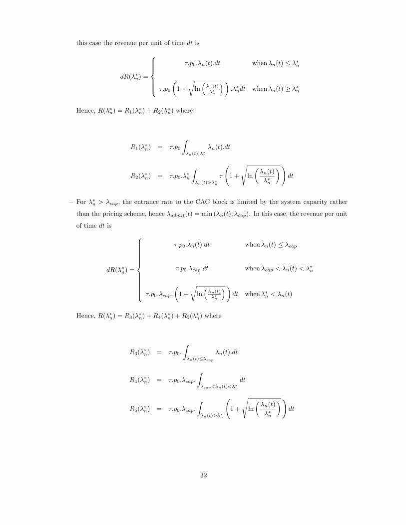
this case the revenue per unit of time dt is

dR(λ∗n) =

τ.p0.λn(t).dt when λn(t) ≤ λ∗n

τ.p0

(

1 +

√

ln(

λn(t)λ∗

n

)

)

.λ∗ndt when λn(t) ≥ λ∗

n

Hence, R(λ∗n) = R1(λ

∗n) + R2(λ

∗n) where

R1(λ∗n) = τ.p0

∫

λn(t)¡λ∗

n

λn(t).dt

R2(λ∗n) = τ.p0.λ

∗n

∫

λn(t)>λ∗

n

τ

(

1 +

√

ln

(

λn(t)

λ∗n

)

)

dt

– For λ∗n > λcap, the entrance rate to the CAC block is limited by the system capacity rather

than the pricing scheme, hence λadmit(t) = min (λn(t), λcap). In this case, the revenue per unit

of time dt is

dR(λ∗n) =

τ.p0.λn(t).dt when λn(t) ≤ λcap

τ.p0.λcap.dt when λcap < λn(t) < λ∗n

τ.p0.λcap.

(

1 +

√

ln(

λn(t)λ∗

n

)

)

dt when λ∗n < λn(t)

Hence, R(λ∗n) = R3(λ

∗n) + R4(λ

∗n) + R5(λ

∗n) where

R3(λ∗n) = τ.p0.

∫

λn(t)≤λcap

λn(t).dt

R4(λ∗n) = τ.p0.λcap.

∫

λcap<λn(t)<λ∗

n

dt

R5(λ∗n) = τ.p0.λcap.

∫

λn(t)>λ∗

n

(

1 +

√

ln

(

λn(t)

λ∗n

)

)

dt

32

The resulting expression for the revenue is:

R(λ∗n) = τ.p0.

∫

λn(t)≤min(λ∗

n,λcap)

λn(t).dt

+ τ.p0.min(λ∗n, λcap).

∫

λn(t)>min(λ∗

n,λcap)

(

1 +

√

ln

(

max

(

λn(t)

λ∗n

, 1

))

)

dt

Mathematica 4.2 has been used to study the variation of R(λ∗n). It was not possible to obtain an

analytical expression of the derivative of the revenue, therefore the variation of the revenue was

studied qualitatively. As λ∗n increases from zero, it can be seen qualitatively that the revenue will

initially increase as calls enter the network (for λ∗n = 0, no traffic enters the system). The variation

of the revenue is unknown until λ∗n = λcap.

For λcap < λ∗n < λmax, R(λ∗

n) = R3(λ∗n) + R4(λ

∗n) + R5(λ

∗n) where R3(λ

∗n) is independent of λ∗

n, and

the sum R4(λ∗n)+R5(λ

∗n) is a decreasing function of λ∗

n (it is a constant traffic share, which is priced

at the off-peak price when the rate is below λ∗n and at the peak price (which is decreasing with λ∗

n)

otherwise). Hence R(λ∗n) is decreasing for λcap < λ∗

n < λmax.

For λmax < λ∗n, R(λ∗

n) = R3(λ∗n) + R4(λ

∗n) + R5(λ

∗n) where R3(λ

∗n) is independent of λ∗

n, R4(λ∗n) is

a constant and R5(λ∗n) is zero, hence R(λ∗

n) is constant.

This analysis may be validated by considering figure 4.5 (plotted using Mathematica 4.2 ). The value

of λ∗n which optimises the network revenue is approximately λ∗

n = 0.11call/second.

0.05 0.1 0.15 0.2lambdaN* (call/s)

200000

400000

600000

800000

revenue

Figure 4.5: Revenue variations

33

4.4 Utility

In this section, we will establish an expression for the total utility over a day. First, an expression

for the blocking probability is found and a model of the utility of a single user is presented. Finally,

a formula for the total utility is established.

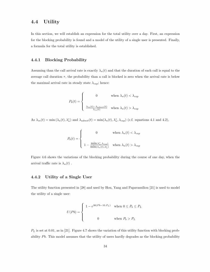
4.4.1 Blocking Probability

Assuming than the call arrival rate is exactly λn(t) and that the duration of each call is equal to the

average call duration τ , the probability than a call is blocked is zero when the arrival rate is below

the maximal arrival rate in steady state λcap; hence:

Pb(t) =

0 when λn(t) < λcap

λin(t)−λadmit(t)λin(t) when λn(t) > λcap

As λin(t) = min (λn(t), λ∗n) and λadmit(t) = min(λn(t), λ∗

n, λcap) (c.f. equations 4.1 and 4.2),

Pb(t) =

0 when λn(t) < λcap

1 −min(λ∗

n,λcap)

min(λn(t),λ∗

n)when λn(t) > λcap

Figure 4.6 shows the variations of the blocking probability during the course of one day, when the

arrival traffic rate is λn(t) .

4.4.2 Utility of a Single User

The utility function presented in [28] and used by Hou, Yang and Papavassiliou [21] is used to model

the utility of a single user:

U(Pb) =

1 − e30(Pb−10.PL) when 0 ≤ Pb ≤ PL

0 when Pb > PL

PL is set at 0.01, as in [21]. Figure 4.7 shows the variation of this utility function with blocking prob-

ability Pb. This model assumes that the utility of users hardly degrades as the blocking probability

34

5 10 15 20t(h)

0.01

0.02

0.03

0.04

0.05

0.06

0.07

Pb

Figure 4.6: Variation of the blocking probability over one day

increases up to a certain limit probability PL. However, after this limit, the utility drops suddenly:

users will not accept the service when the QoS is worse than a pre-specified threshold.

0.002 0.004 0.006 0.008 0.01 0.012Pb

0.2

0.4

0.6

0.8

utility

Figure 4.7: Variation in the utility of a single user with the blocking probability

If we call λL the arrival rate so that P (λL) = PL, then λcap < λL and the utility can be expressed

as:

35

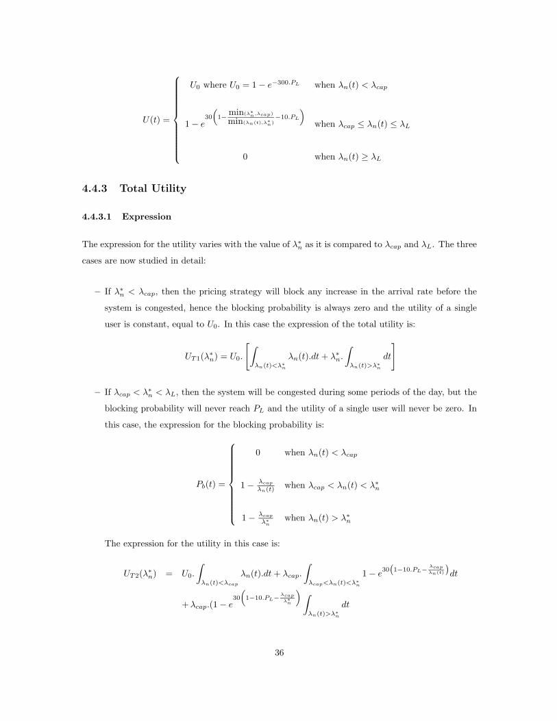
U(t) =

U0 where U0 = 1 − e−300.PL when λn(t) < λcap

1 − e30

(

1−min(λ∗

n,λcap)

min(λn(t),λ∗

n)−10.PL

)

when λcap ≤ λn(t) ≤ λL

0 when λn(t) ≥ λL

4.4.3 Total Utility

4.4.3.1 Expression

The expression for the utility varies with the value of λ∗n as it is compared to λcap and λL. The three

cases are now studied in detail:

– If λ∗n < λcap, then the pricing strategy will block any increase in the arrival rate before the

system is congested, hence the blocking probability is always zero and the utility of a single

user is constant, equal to U0. In this case the expression of the total utility is:

UT1(λ∗n) = U0.

[

∫

λn(t)<λ∗

n

λn(t).dt + λ∗n.

∫

λn(t)>λ∗

n

dt

]

– If λcap < λ∗n < λL, then the system will be congested during some periods of the day, but the

blocking probability will never reach PL and the utility of a single user will never be zero. In

this case, the expression for the blocking probability is:

Pb(t) =

0 when λn(t) < λcap

1 −λcap

λn(t) when λcap < λn(t) < λ∗n

1 −λcap

λ∗

nwhen λn(t) > λ∗

n

The expression for the utility in this case is:

UT2(λ∗n) = U0.

∫

λn(t)<λcap

λn(t).dt + λcap.

∫

λcap<λn(t)<λ∗

n

1 − e30

(

1−10.PL−λcap

λn(t)

)

dt

+λcap.(1 − e30

(

1−10.PL−λcap

λ∗

n

)

∫

λn(t)>λ∗

n

dt

36

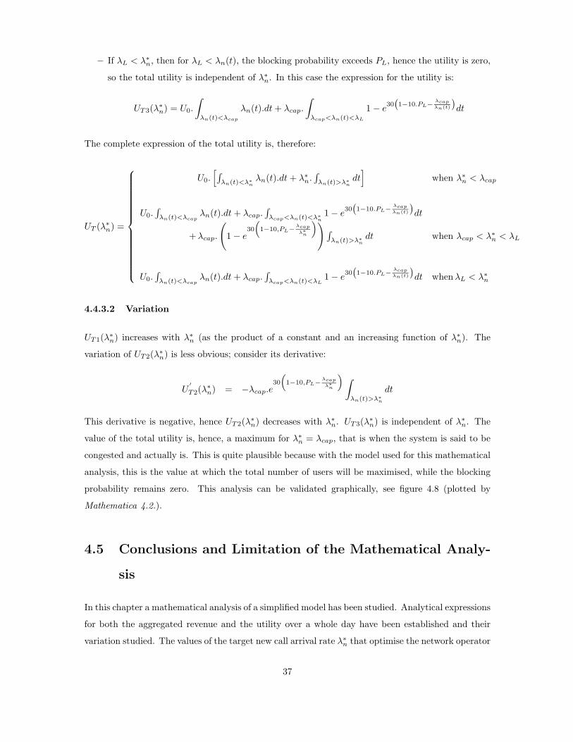
– If λL < λ∗n, then for λL < λn(t), the blocking probability exceeds PL, hence the utility is zero,

so the total utility is independent of λ∗n. In this case the expression for the utility is:

UT3(λ∗n) = U0.

∫

λn(t)<λcap

λn(t).dt + λcap.

∫

λcap<λn(t)<λL

1 − e30

(

1−10.PL−λcap

λn(t)

)

dt

The complete expression of the total utility is, therefore:

UT (λ∗n) =

U0.[

∫

λn(t)<λ∗

nλn(t).dt + λ∗

n.∫

λn(t)>λ∗

ndt

]

when λ∗n < λcap

U0.∫

λn(t)<λcapλn(t).dt + λcap.

∫

λcap<λn(t)<λ∗

n1 − e

30(

1−10.PL−λcap

λn(t)

)

dt

+λcap.

(

1 − e30

(

1−10,PL−λcap

λ∗

n

)

)

∫

λn(t)>λ∗

ndt when λcap < λ∗

n < λL

U0.∫

λn(t)<λcapλn(t).dt + λcap.

∫

λcap<λn(t)<λL1 − e

30(

1−10.PL−λcap

λn(t)

)

dt when λL < λ∗n

4.4.3.2 Variation

UT1(λ∗n) increases with λ∗

n (as the product of a constant and an increasing function of λ∗n). The

variation of UT2(λ∗n) is less obvious; consider its derivative:

U′

T2(λ∗n) = −λcap.e

30

(

1−10,PL−λcap

λ∗

n

)

∫

λn(t)>λ∗

n

dt

This derivative is negative, hence UT2(λ∗n) decreases with λ∗

n. UT3(λ∗n) is independent of λ∗

n. The

value of the total utility is, hence, a maximum for λ∗n = λcap, that is when the system is said to be

congested and actually is. This is quite plausible because with the model used for this mathematical

analysis, this is the value at which the total number of users will be maximised, while the blocking

probability remains zero. This analysis can be validated graphically, see figure 4.8 (plotted by

Mathematica 4.2.).

4.5 Conclusions and Limitation of the Mathematical Analy-

sis

In this chapter a mathematical analysis of a simplified model has been studied. Analytical expressions

for both the aggregated revenue and the utility over a whole day have been established and their

variation studied. The values of the target new call arrival rate λ∗n that optimise the network operator

37

0.05 0.1 0.15 0.2lambdaN*(call/s)

1000

2000

3000

4000Pb

Figure 4.8: Variations in total utility

revenue and the total utility of users differ significantly (0.11 and 0.1375 respectively). Therefore, a

trade-off has to be found between maximising the network operator revenue and the total utility of

users.

This analysis suggests that there are optimal values for the target new call arrival rate that max-

imises the network operator revenue and the total utility and that these may differ. However, the

simplifications and assumptions used to make this model tractable mean that it might not repre-

sent the network completely. We review each of the assumptions made and examine their potential

impact on the results above.

This model does not include hand-off calls. This should mainly influence the blocking probability,

as in the real scheme this is a weighted average of the hand-off and new call blocking probability

(these are different due to the CAC scheme used).

It is also assumed that the regulation by the price is perfect; this will lead to a reduction in the

blocking probability when compared with the modelled system. This effect will be increased by the

simplification used to model the system as a succession of steady states. The assumption that all

calls last for the same length of time smoothes the variations of the blocking probability and, hence,

the price. The fact that the arrival of the calls is assumed to be an arrival of rate exactly λn(t) and

not a Poisson process of mean λn(t) will augment this effect. When considering the revenue, these

variations should be averaged, whereas for the total utility, because of the preset threshold value,

the result may differ significantly.

Finally, the assumption that all hold-off or blocked users leave the system could lead to a reduced

blocking probability, hence an increased utility and a reduced revenue in comparison to the real

38

system.

For these reasons, the validity of the above mathematical model may be questionable. The main

concern relates to the blocking probability, which influences in particular the total utility. In the

following chapters, the simulator implemented, the model designed and the results obtained by

simulations are described and analysed.

39

Chapter 5

Simulator Description

Having examined existing network models and analysed a simple analytical model, the motivations

for using and writing a simulator are now presented together with the specification and design of the

simulator written. Some detail relating to its technical features are given and the chapter concludes

with a description of the process used to validate the simulator.

5.1 Motivations

5.1.1 Motivations for Using a Simulator

Cellular networks are complex systems, not only due to their structure but also due to the complexity

of their traffic. A cellular network covers a broad geographical area which is divided into cells. Users

may migrate between cells while making or receiving phone calls. When a request to start or continue

a call in a cell is made, the network has to decide if it will assign the necessary resources to this

call or reject it. This will depend on the current traffic in the system. The traffic generated in cells

may vary both temporally and spatially. The mobility of users makes the specification of the total

traffic in the network even more complex. This complexity is hard to model mathematically: treated

in isolation each element may be successfully modelled, but their combination cannot be, especially

when considering a large number of cells. Whereas an approximate analytical formulation and its

solution can be useful for designing algorithms and getting a detailed understanding of how they

influence the traffic, their evaluation requires testing with more accurate models. It is particularly

difficult to run practical experiments of such scope, hence the use of simulation provides a useful

solution: the system may be modelled in great detail while still providing a suitable environment for

testing algorithms.

40

5.1.2 Motivations for Writing a new Simulator

Simulation is used in a wide variety of research domains and a large number of simulators are available

for use. Whereas several simulators of computer networks exist, the number of simulators for cellular

networks is much smaller. The simulator required for this work needs to handle call generation, call

admission, resource management and mobility of users in a cellular network.

Some of the big multi-purpose simulators include a GSM/GPRS module. For example, a GPRS

module [23] for the widely used simulator NS2 [4] is available. However this module aims to model

low level communication (packet level) and does not provide higher functionality such as resource

management or call hand-off. While extending the simulator to provide these functionalities is

possible, the fact that the simulator handles so many low level details makes it exceedingly slow to

obtain meaningful results when using it for the purpose of this study. Furthermore, as this module

has not been designed to handle several cells, extending it to provide this functionality could prove

problematic. The commercial simulator OPNET also includes a GPRS module, but it also does not

support hand-off between cells.

The lack of an adequate simulator meant it was either necessary to extend an existing one or write

one from scratch. The low-level nature of existing simulators means it is very slow to compute many

higher level operations, so the decision to write a new simulator was made.

5.2 Specifications

The focus of this work is on pricing in cellular networks, and any simulator written must include the

following features:

– cellular network traffic generation,

– call admission,

– resource management,

– call mobility,

– pricing.

The simulator should be able to model several cells over several days, with a time- and space-

dependent traffic generation rate . It should also be possible to measure several performance metrics

such as the variation of traffic, price and revenue over a variety of time periods.

41

5.3 Design

5.3.1 Level of Abstraction

For a simulation model to be accurate and efficient, the correct level of detail required needs to be

determined as a function of both the specific issues to be investigated and the evaluation methodology

used. As for this work focuses on resource management, the level of abstraction chosen is the

individual call: to evaluate the resource management at the channel level, it is not necessary to

know the number of packets sent, as a channel is reserved for each call during its entire duration.

5.3.2 Different Simulator Types

A simulator can either model events discreetly or using a continuous, fluid model. In the first case,

each event is simulated, while in the second case the global behaviour of several events is considered.

The first method is the closest to real network behaviour, however the second method may be more

efficient for modelling a large number of events.

The simulator can be either event-driven or time driven. An event-driven simulator is continuous:

each event is processed one after the other, with the simulation clock advancing from one event time

to the next. In a time driven simulator, time is split into small intervals, and the simulator clock

advances by fixed increments; hence the simulation is discrete. At the end of each time interval,

the state of the system is updated with the results of all the events that are scheduled during the

interval. Event-driven simulation can produce results with a great level of precision; on the other

hand time-driven simulator can be easily implemented on a parallel architecture, hence reducing the

execution time.

The number of calls per cell per day is bounded by the cell capacity and the call level abstraction

makes it feasible to simulate each call. Hence, for this work, it has been chosen to write a discrete

event, event-driven simulator .

5.3.3 Different Types of Events

In this simulator, the different events are the start or end of a phone call or GPRS session. The four

different events types occurring during the simulation are EventStartGSM and EventStartGPRS

that model the beginning of a GSM call and a GPRS session respectively and EventCloseGSM

and EventCloseGPRS which model the corresponding end of calls or session. Figure 5.1 shows the

hierarchy of the different type of events.

42

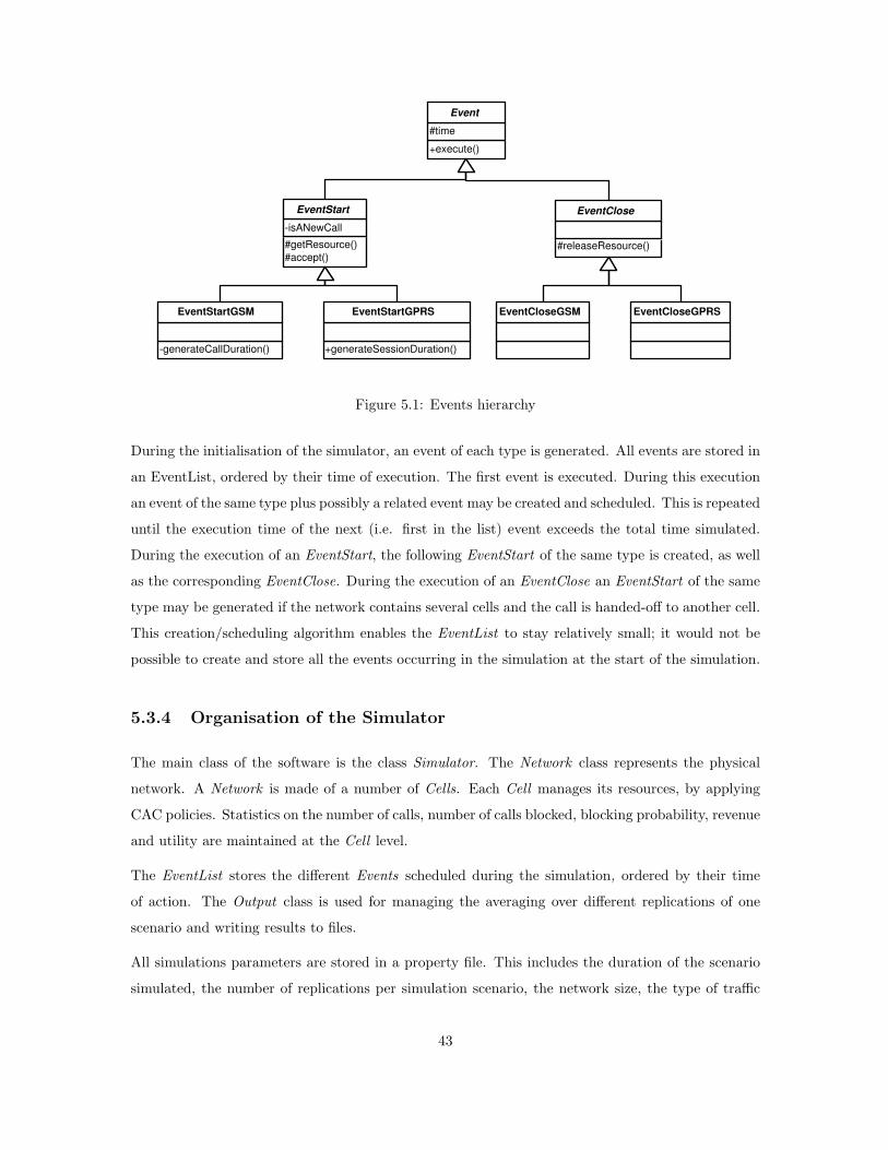
+execute()

#time

Event

#getResource()

#accept()

-isANewCall

EventStart

#releaseResource()

EventClose

-generateCallDuration()

EventStartGSM

+generateSessionDuration()

EventStartGPRS EventCloseGSM EventCloseGPRS

Figure 5.1: Events hierarchy

During the initialisation of the simulator, an event of each type is generated. All events are stored in

an EventList, ordered by their time of execution. The first event is executed. During this execution

an event of the same type plus possibly a related event may be created and scheduled. This is repeated

until the execution time of the next (i.e. first in the list) event exceeds the total time simulated.

During the execution of an EventStart, the following EventStart of the same type is created, as well

as the corresponding EventClose. During the execution of an EventClose an EventStart of the same

type may be generated if the network contains several cells and the call is handed-off to another cell.

This creation/scheduling algorithm enables the EventList to stay relatively small; it would not be

possible to create and store all the events occurring in the simulation at the start of the simulation.

5.3.4 Organisation of the Simulator

The main class of the software is the class Simulator. The Network class represents the physical

network. A Network is made of a number of Cells. Each Cell manages its resources, by applying

CAC policies. Statistics on the number of calls, number of calls blocked, blocking probability, revenue

and utility are maintained at the Cell level.

The EventList stores the different Events scheduled during the simulation, ordered by their time

of action. The Output class is used for managing the averaging over different replications of one

scenario and writing results to files.

All simulations parameters are stored in a property file. This includes the duration of the scenario

simulated, the number of replications per simulation scenario, the network size, the type of traffic

43

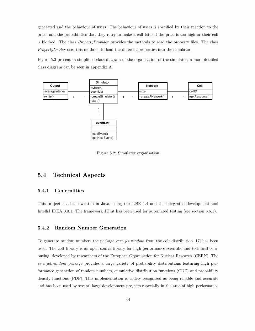
generated and the behaviour of users. The behaviour of users is specified by their reaction to the

price, and the probabilities that they retry to make a call later if the price is too high or their call

is blocked. The class PropertyProvider provides the methods to read the property files. The class

PropertyLoader uses this methods to load the different properties into the simulator.

Figure 5.2 presents a simplified class diagram of the organisation of the simulator; a more detailed

class diagram can be seen in appendix A.

+createSimulator()

+start()

-network

-eventList

Simulator

+createANetwork()

-size

Network

1 1

+addEvent()

+getNextEvent()

eventList

+getResource()

-cellID

Cell

1 *

1

1

+write()

-averageInterval

Output

1 *

Figure 5.2: Simulator organisation

5.4 Technical Aspects

5.4.1 Generalities

This project has been written in Java, using the J2SE 1.4 and the integrated development tool

IntelliJ IDEA 3.0.1. The framework JUnit has been used for automated testing (see section 5.5.1).

5.4.2 Random Number Generation

To generate random numbers the package cern.jet.random from the colt distribution [17] has been

used. The colt library is an open source library for high performance scientific and technical com-

puting, developed by researchers of the European Organisation for Nuclear Research (CERN). The

cern.jet.random package provides a large variety of probability distributions featuring high per-

formance generation of random numbers, cumulative distribution functions (CDF) and probability

density functions (PDF). This implementation is widely recognised as being reliable and accurate

and has been used by several large development projects especially in the area of high performance

44

numerical analysis (for example in the Scalable Simulation Framework [2]). It has no known bugs.

However, to check the correct use of this implementation, all functions used have been extensively

tested (see section 5.5.1) prior to their use in this work.

5.4.3 Arrival Rate Modelling

As explained in chapter 3, the call arrival rate is modelled by a Poisson process with a non-stationary

rate λn(t). Generating arrival times t1, t2, t3... that follow a non-stationary Poisson process is

significantly complex: the first intuition would be to generate ti+1 from ti by generating a variable

that follows an exponential distribution of rate 1/λn(ti) (as, by definition, inter-arrival times of a

Poisson process of rate λ follow an exponential distribution of mean 1/λ), however this is not valid,

as it would ignore the variation of λn(t) between ti and ti+1. Therefore, special care should be given

to this task. In the simulator, an algorithm [36] inspired of the thinning algorithm presented in [31]

has been used. These algorithms work if λmax = max(λ(t)) is finite. The principle is to generate a

stationary Poisson process with a constant rate λmax and arrival times {tmaxi } and rejecting each

tmaxi as an arrival with the probability 1 − λ (tmax

i ) /λmax. Thus, it is more likely that an arrival

time tmaxi is accepted if λ (tmax

i ) is high, yielding the desired property that arrivals will occur more

frequently in intervals for which λ(t) is high [36]. The different steps of the algorithm used are the

following:

1. Set t = ti−1.

2. Generate U1 and U2 as two uniformly distributed independent variates.

3. Replace t by t − (1/λmax) ln (U1).

4. If U2 ≤ λn(t)/λmax, return t = ti. Otherwise, go back to step 2.

5.5 Validation

Building a simulator is an easy task; building a valid and credible simulator is much harder, as every

detail of the model chosen need to be implemented and it can be extremely difficult to detect errors.

While it is vital to chose an appropriate abstraction model and simulator type, it is also crucial to

control the development of the simulator. To this end, several tests and verification procedures have

been used in the course of this work, and the simulator has been used to reproduce existing results

from previous experiments.

45

5.5.1 Tests

This simulator has been developed using test-first programming, as this enables a high level of

confidence in the resulting system. While defining each function, a test was written for every specific

case of the function. The statistical variable generators for each distribution used have also been

tested, with a verification of the mean and variance. Moreover each time a generator was used in

the simulator, it has been tested that the results were as expected. The use of systematic automatic

tests is a crucial factor in the building of such a system, as it avoids numerous errors that may not

be easily detected otherwise.

In addition to function testing, several trace analyses have been conducted. These check step by step,

by hand calculation, that the system behaviour is correct. Furthermore, the system has been built

incrementally, starting with the simplest case and adding features and details, hence simple cases

have been tested with different versions of the simulator and the output checked against analytical

results.

5.5.2 Results Reproduction

To ensure than the simulator produces valid results, and to perform a complex global test, the five

experiments described in [21] have been simulated and the results have been compared with the

one given in this article. The similarity of the results produced is a good gage of the validity and

accuracy of the simulator written.

5.6 Conclusion

In this chapter, a general overview of the simulator has been presented and the challenging technical

aspects detailed. In the following chapter, the experiments run on this simulator and their results

will be discussed.

46

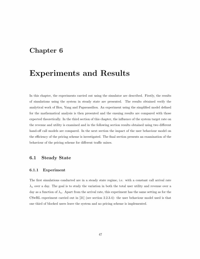
Chapter 6

Experiments and Results

In this chapter, the experiments carried out using the simulator are described. Firstly, the results

of simulations using the system in steady state are presented. The results obtained verify the

analytical work of Hou, Yang and Papavassiliou. An experiment using the simplified model defined

for the mathematical analysis is then presented and the ensuing results are compared with those

expected theoretically. In the third section of this chapter, the influence of the system target rate on

the revenue and utility is examined and in the following section results obtained using two different

hand-off call models are compared. In the next section the impact of the user behaviour model on

the efficiency of the pricing scheme is investigated. The final section presents an examination of the

behaviour of the pricing scheme for different traffic mixes.

6.1 Steady State

6.1.1 Experiment

The first simulations conducted are in a steady state regime, i.e. with a constant call arrival rate

λn over a day. The goal is to study the variation in both the total user utility and revenue over a

day as a function of λn. Apart from the arrival rate, this experiment has the same setting as for the

CSwRL experiment carried out in [21] (see section 2.2.3.4): the user behaviour model used is that

one third of blocked users leave the system and no pricing scheme is implemented.

47

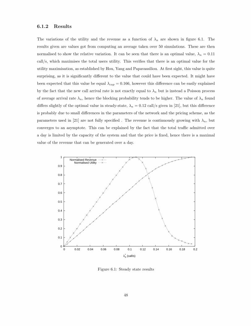
6.1.2 Results

The variations of the utility and the revenue as a function of λn are shown in figure 6.1. The

results given are values got from computing an average taken over 50 simulations. These are then

normalised to show the relative variation. It can be seen that there is an optimal value, λn = 0.11

call/s, which maximises the total users utility. This verifies that there is an optimal value for the

utility maximisation, as established by Hou, Yang and Papavassiliou. At first sight, this value is quite

surprising, as it is significantly different to the value that could have been expected. It might have

been expected that this value be equal λcap = 0.166, however this difference can be easily explained

by the fact that the new call arrival rate is not exactly equal to λn but is instead a Poisson process

of average arrival rate λn, hence the blocking probability tends to be higher. The value of λn found

differs slightly of the optimal value in steady-state, λn = 0.12 call/s given in [21], but this difference

is probably due to small differences in the parameters of the network and the pricing scheme, as the

parameters used in [21] are not fully specified . The revenue is continuously growing with λn, but

converges to an asymptote. This can be explained by the fact that the total traffic admitted over

a day is limited by the capacity of the system and that the price is fixed, hence there is a maximal

value of the revenue that can be generated over a day.

0

0.1

0.2

0.3

0.4

0.5

0.6

0.7

0.8

0.9

1

0 0.02 0.04 0.06 0.08 0.1 0.12 0.14 0.16 0.18 0.2

λ*n (call/s)

Normalised RevenueNormalised Utility

Figure 6.1: Steady state results

48

6.2 Results Corresponding to the Model Used for the Ana-

lytical Analysis

6.2.1 Experiment

For direct comparison with the results of the mathematical analysis presented in chapter 4, an

experiment has been run using the traffic model which the mathematical formulae are based on.

This model does not include hand-off calls and it is assumed that all blocked users and those who

find the price too high leave the system. We study the variation of the total utility and revenue over

a day, as a function of λ∗n.

To obtain comparable results for the case where hand-off calls are included, the total capacity of the

system is divided by the ratio of the mean call holding time and the mean cell dwell time, as this is

an approximation for the formulae 3.3.1.

6.2.2 Results

The results have been averaged over 100 experiments. Figure 6.2 shows the normalised variation of

the total utility and the revenue over a day for different values of λ∗n (in calls per second). The total

utility is maximised for λ∗n = 0.11 calls/s whereas the revenue is maximised for λ∗

n = 0.1 calls/s. This

means than a trade-off has to be found between the two maximisation objectives. The value of λ∗nthat

optimises the revenue is fairly close to the one expected according to the mathematical analysis. The

value of λ∗n that optimises the total users utility is slightly smaller than the one presented in the

mathematical analysis. This is may be attributed to the simplifications and assumptions used in the

mathematical analysis, as explained in section 4.5.

6.2.3 Conclusion

These results suggest that the mathematical analysis provided accurate results for the simplified

models used. Furthermore, as it will be seen in the following sections, these results are quite close to

the one of the complete models. The presence of hand-off calls, however, changes slightly the shape

of the utility function.

49

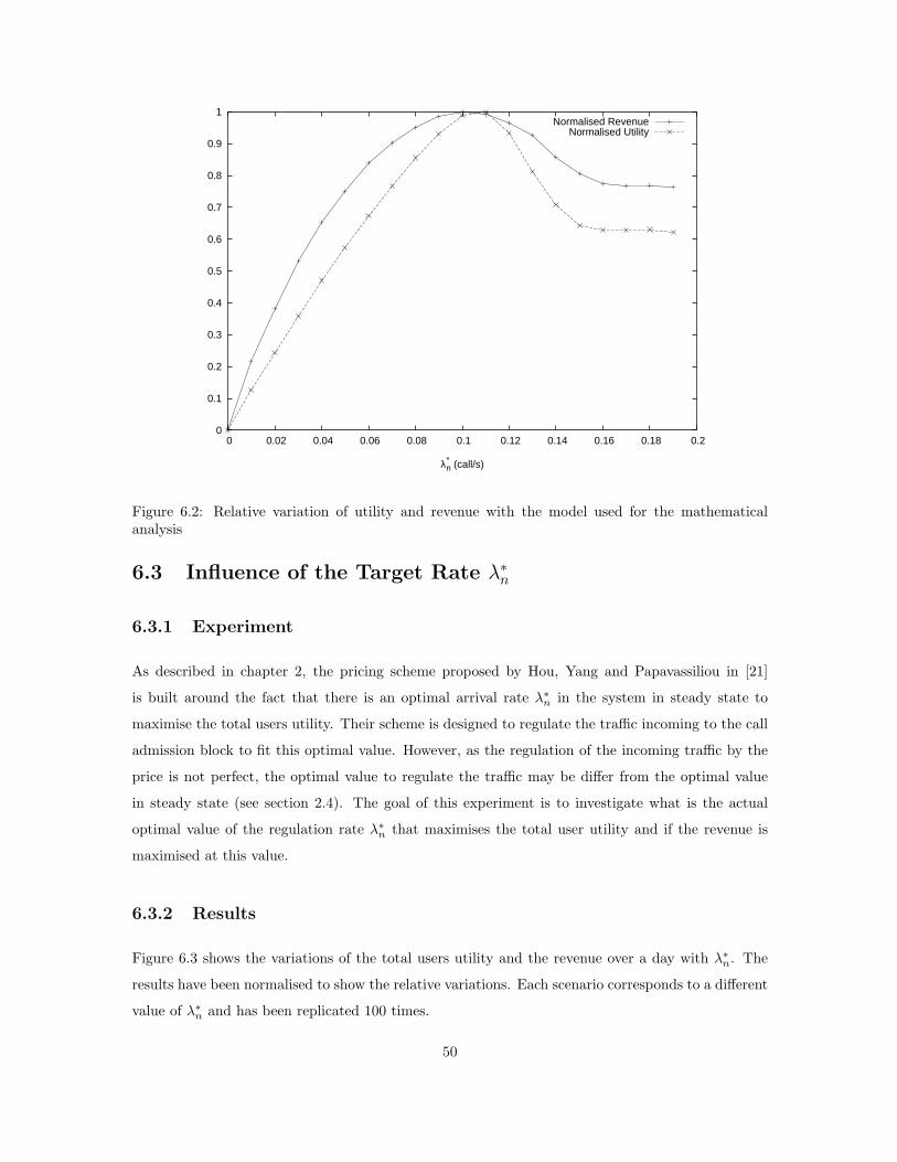
0

0.1

0.2

0.3

0.4

0.5

0.6

0.7

0.8

0.9

1

0 0.02 0.04 0.06 0.08 0.1 0.12 0.14 0.16 0.18 0.2

λ*n (call/s)

Normalised RevenueNormalised Utility

Figure 6.2: Relative variation of utility and revenue with the model used for the mathematicalanalysis

6.3 Influence of the Target Rate λ∗n

6.3.1 Experiment

As described in chapter 2, the pricing scheme proposed by Hou, Yang and Papavassiliou in [21]

is built around the fact that there is an optimal arrival rate λ∗n in the system in steady state to

maximise the total users utility. Their scheme is designed to regulate the traffic incoming to the call

admission block to fit this optimal value. However, as the regulation of the incoming traffic by the

price is not perfect, the optimal value to regulate the traffic may be differ from the optimal value

in steady state (see section 2.4). The goal of this experiment is to investigate what is the actual

optimal value of the regulation rate λ∗n that maximises the total user utility and if the revenue is

maximised at this value.

6.3.2 Results

Figure 6.3 shows the variations of the total users utility and the revenue over a day with λ∗n. The

results have been normalised to show the relative variations. Each scenario corresponds to a different

value of λ∗n and has been replicated 100 times.

50

0

0.1

0.2

0.3

0.4

0.5

0.6

0.7

0.8

0.9

1

0 0.02 0.04 0.06 0.08 0.1 0.12 0.14 0.16 0.18 0.2

λ*n (call/s)

Normalised RevenueNormalised Utility

Figure 6.3: Variation of the total users utility and the total revenue over a day with λ∗n

It can be seen that there an optimal value of λ∗n to maximise the utility and one to maximise the

network operator revenue. This could have been predicted as the total user utility will increase

with the number of users admitted to the network, hence with λ∗n, but after a point the blocking

probability will become higher than the limit value PL and the utility of the admitted users will be

zero. Similarly, with the revenue, it will first grow with the number of users admitted to the system,

but will then decrease as the fraction of users charged a peak-price will decrease.

It should be noticed than the value of λ∗n that maximises the total users utility is really close to the

one that maximises the network operator revenue. This is due to the fact than the pricing scheme

is designed to maximise the total users utility and furthermore that during the simulations, the user

behaviour is modelled using the model used for the defining the pricing scheme (this means than the

users act exactly as expected).

Furthermore, the optimal value λ∗n= 0.10 call/s which maximises the total users utility and the

revenue is significantly different than the optimal value in steady state (λ∗n= 0.11 call/s). The

difference in term of revenue and utility are in the order of approximately 1%. This is not a major

difference but is not negligible, especially when considering the revenue.

51

6.4 Influence of the Hand-off Call Model

6.4.1 Experiments

The goal of these experiments is to compare the results obtained using the two different hand-off

call models: modelling and generation by running simulations on several cells (see section 3.3). The

simulations run over several cells are run on 19 neighbouring cells, using the wrapped around model.

Two experiments have been carried out: the first one compares the variations of the new call arrival

and admission rates and the hand-off call arrival rate during the day for each of the two hand-off

models. The second experiment aims to compare the variations of the total users utility and the

total revenue over a day with λ∗n for each model. The settings for all experiments corresponds to

those of the PSwRL experiment (see section 2.2.3.4).

6.4.2 Results

Figure 6.4 shows the variation of the new call arrival and admission rates and the hand-off call arrival

rate during the day using the two hand-off models. The results are averaged over 10 simulations. It

can be seen that the two models are fairly close.

The variation of the total users utility and the total revenue over a day with λ∗n with the two hand-off

models are showed in figures 6.5 and 6.6 respectively. Each scenario has been replicated 10 times.

These figures show that the results for the two models are really similar.

6.4.3 Conclusion

The two experiments carried out show that both the results at small scale (every five minutes) and

large scale (total for one day) using the two different models for hand-off calls are very similar. This

validates the formula used to model the hand-off arrival rate (equation 3.1). As the model using

several cells requires significantly more time for each simulation, for other experiments the model

with a single cell is used.

6.5 Influence of Call Holding Time Model

6.5.1 Motivations

In Hou, Yang and Papavassiliou’s experiments, the call duration (call holding time) is assumed to

be independent of the price. They justify this assumption by referring to the practical experiments

52

0

0.05

0.1

0.15

0.2

0.25

0.3

0 5 10 15 20

call/

s

Time of the day (h)

λn - multiple cellsλh - multiple cells

λadmit - multiple cellsλn - one cellλh - one cell

λadmit - one cell

Figure 6.4: Variations of the new call arrival and admission and the hand-off call arrival rate duringthe day with the two models of hand-off calls studied

0

500000

1e+06

1.5e+06

2e+06

2.5e+06

3e+06

0 0.02 0.04 0.06 0.08 0.1 0.12 0.14 0.16 0.18 0.2

Rev

enue

λ*n (call/s)

One cellMultiple cells

Figure 6.5: Variations of the total revenue over a day in function of λ∗n with both hand-off models

53

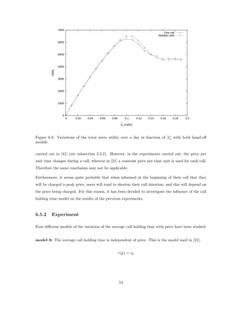
0

1000

2000

3000

4000

5000

6000

7000

0 0.02 0.04 0.06 0.08 0.1 0.12 0.14 0.16 0.18 0.2

Util

ity

λ*n (call/s)

One cellMultiple cells

Figure 6.6: Variations of the total users utility over a day in function of λ∗n with both hand-off

models

carried out in [41] (see subsection 2.3.2). However, in the experiments carried out, the price per

unit time changes during a call, whereas in [21] a constant price per time unit is used for each call.

Therefore the same conclusion may not be applicable.

Furthermore, it seems quite probable that when informed at the beginning of their call that they

will be charged a peak price, users will tend to shorten their call duration, and this will depend on

the price being charged. For this reason, it has been decided to investigate the influence of the call

holding time model on the results of the previous experiments.

6.5.2 Experiment

Four different models of the variation of the average call holding time with price have been studied:

model 0: The average call holding time is independent of price. This is the model used in [21].

τ(p) = τ0

54

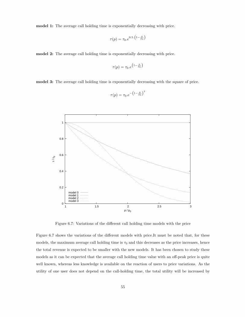
model 1: The average call holding time is exponentially decreasing with price.

τ(p) = τ0.e0.5.

(

1− p

p0

)

model 2: The average call holding time is exponentially decreasing with price.

τ(p) = τ0.e

(

1− p

p0

)

model 3: The average call holding time is exponentially decreasing with the square of price.

τ(p) = τ0.e−(

1− p

p0

)2

0

0.2

0.4

0.6

0.8

1

1 1.5 2 2.5 3

τ / τ

0

p / p0

model 0model 1model 2model 3

Figure 6.7: Variations of the different call holding time models with the price

Figure 6.7 shows the variations of the different models with price.It must be noted that, for these

models, the maximum average call holding time is τ0 and this decreases as the price increases, hence

the total revenue is expected to be smaller with the new models. It has been chosen to study these

models as it can be expected that the average call holding time value with an off-peak price is quite

well known, whereas less knowledge is available on the reaction of users to price variations. As the

utility of one user does not depend on the call-holding time, the total utility will be increased by

55

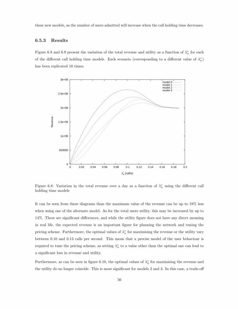
these new models, as the number of users admitted will increase when the call holding time decreases.

6.5.3 Results

Figure 6.8 and 6.9 present the variation of the total revenue and utility as a function of λ∗n for each

of the different call holding time models. Each scenario (corresponding to a different value of λ∗n)

has been replicated 10 times.

0

500000

1e+06

1.5e+06

2e+06

2.5e+06

3e+06

0 0.02 0.04 0.06 0.08 0.1 0.12 0.14 0.16 0.18 0.2

Rev

enue

λ*n (call/s)

model 0model 1model 2model 3

Figure 6.8: Variation in the total revenue over a day as a function of λ∗n using the different call

holding time models

It can be seen from these diagrams than the maximum value of the revenue can be up to 18% less

when using one of the alternate model. As for the total users utility, this may be increased by up to

14%. These are significant differences, and while the utility figure does not have any direct meaning

in real life, the expected revenue is an important figure for planning the network and tuning the

pricing scheme. Furthermore, the optimal values of λ∗n for maximising the revenue or the utility vary

between 0.10 and 0.13 calls per second. This mean that a precise model of the user behaviour is

required to tune the pricing scheme, as setting λ∗n to a value other than the optimal one can lead to

a significant loss in revenue and utility.

Furthermore, as can be seen in figure 6.10, the optimal values of λ∗n for maximising the revenue and

the utility do no longer coincide. This is most significant for models 2 and 3. In this case, a trade-off

56

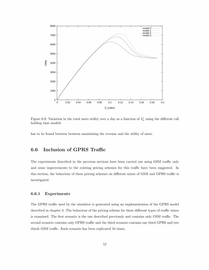
0

1000

2000

3000

4000

5000

6000

7000

8000

0 0.02 0.04 0.06 0.08 0.1 0.12 0.14 0.16 0.18 0.2

Util

ity

λ*n (call/s)

model 0model 1model 2model 3

Figure 6.9: Variation in the total users utility over a day as a function of λ∗n using the different call

holding time models

has to be found between between maximising the revenue and the utility of users.

6.6 Inclusion of GPRS Traffic

The experiments described in the previous sections have been carried out using GSM traffic only

and some improvements to the existing pricing schemes for this traffic have been suggested. In

this section, the behaviour of these pricing schemes on different mixes of GSM and GPRS traffic is

investigated.

6.6.1 Experiments

The GPRS traffic used by the simulator is generated using an implementation of the GPRS model

described in chapter 3. The behaviour of the pricing scheme for three different types of traffic mixes

is examined. The first scenario is the one described previously and contains only GSM traffic. The

second scenario contains only GPRS traffic and the third scenario contains one third GPRS and two

thirds GSM traffic. Each scenario has been replicated 10 times.

57

0

0.1

0.2

0.3

0.4

0.5

0.6

0.7

0.8

0.9

1

0 0.02 0.04 0.06 0.08 0.1 0.12 0.14 0.16 0.18 0.2

λ*n (call/s)

Normalised RevenueNormalised Utility

0

0.1

0.2

0.3

0.4

0.5

0.6

0.7

0.8

0.9

1

0 0.02 0.04 0.06 0.08 0.1 0.12 0.14 0.16 0.18 0.2

λ*n (call/s)

Normalised RevenueNormalised Utility

0

0.1

0.2

0.3

0.4

0.5

0.6

0.7

0.8

0.9

1

0 0.02 0.04 0.06 0.08 0.1 0.12 0.14 0.16 0.18 0.2

λ*n (call/s)

Normalised RevenueNormalised Utility

Figure 6.10: Variations of the revenue and the total users utility as a function of λ∗n for the call-

holding time model 1 (top), model 2 (centre) and model 3 (bottom)

58

According to the GPRS traffic model described in chapter 3, the mean session duration of GPRS

traffic is significantly higher than the mean call holding time for GSM traffic. This means that for

the same traffic volume in the system, less GPRS calls are admitted. Hence the pricing scheme has

been adapted by sizing the value of the target arrival rate by the ratio of the two mean durations,

so that the traffic scheme will have similar effect on both types of traffic.

6.6.2 Results

As the total utility function, defined in section 4.4.3, is not dependent on the duration of the calls,

but rather on the number of calls admitted, the total utility will be significantly smaller for GPRS

traffic. This is demonstrated in figure 6.11, which shows the total utility for each of the scenarios.

This figure also shows that for the mix of both GPRS and GSM traffic, the total utility reaches a

steady state instead of declining from a maximum as for the other scenarios. The revenue generated

by each of the schemes is shown on figure 6.12. It can be seen that the revenue is lower for single

type traffic mixes. This is due to the fact that there are two separate prices for the two traffic types,

and that they will not increase as much if there are less traffic of their type.

0

1000

2000

3000

4000

5000

6000

7000

0 0.02 0.04 0.06 0.08 0.1 0.12 0.14 0.16 0.18 0.2

Util

ity

λ*n (call/s)

GSMGPRS

GSM + GPRS

Figure 6.11: Comparison of the utility for each of the traffic mixes

Figure 6.13 shows the normalised variation of the revenue and the utility for each of the scenarios. It

can be seen that if the pricing scheme provides a single value of target incoming rate for optimising

59

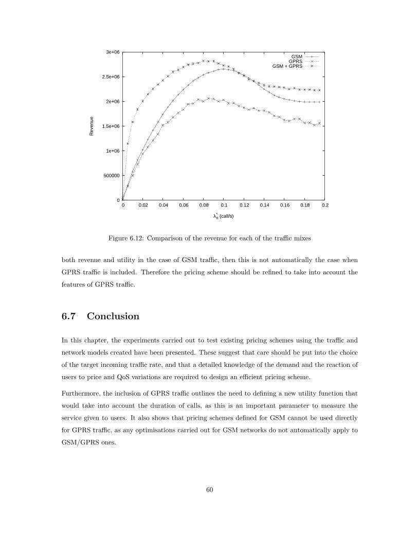
0

500000

1e+06

1.5e+06

2e+06

2.5e+06

3e+06

0 0.02 0.04 0.06 0.08 0.1 0.12 0.14 0.16 0.18 0.2

Rev

enue

λ*n (call/s)

GSMGPRS

GSM + GPRS

Figure 6.12: Comparison of the revenue for each of the traffic mixes

both revenue and utility in the case of GSM traffic, then this is not automatically the case when

GPRS traffic is included. Therefore the pricing scheme should be refined to take into account the

features of GPRS traffic.

6.7 Conclusion

In this chapter, the experiments carried out to test existing pricing schemes using the traffic and

network models created have been presented. These suggest that care should be put into the choice

of the target incoming traffic rate, and that a detailed knowledge of the demand and the reaction of

users to price and QoS variations are required to design an efficient pricing scheme.

Furthermore, the inclusion of GPRS traffic outlines the need to defining a new utility function that

would take into account the duration of calls, as this is an important parameter to measure the

service given to users. It also shows that pricing schemes defined for GSM cannot be used directly

for GPRS traffic, as any optimisations carried out for GSM networks do not automatically apply to

GSM/GPRS ones.

60

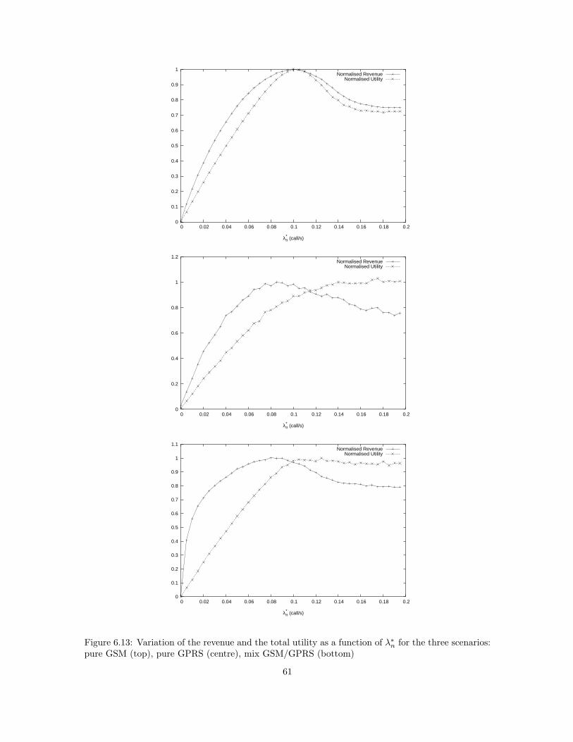
0

0.1

0.2

0.3

0.4

0.5

0.6

0.7

0.8

0.9

1

0 0.02 0.04 0.06 0.08 0.1 0.12 0.14 0.16 0.18 0.2

λ*n (call/s)

Normalised RevenueNormalised Utility

0

0.2

0.4

0.6

0.8

1

1.2

0 0.02 0.04 0.06 0.08 0.1 0.12 0.14 0.16 0.18 0.2

λ*n (call/s)

Normalised RevenueNormalised Utility

0

0.1

0.2

0.3

0.4

0.5

0.6

0.7

0.8

0.9

1

1.1

0 0.02 0.04 0.06 0.08 0.1 0.12 0.14 0.16 0.18 0.2

λ*n (call/s)

Normalised RevenueNormalised Utility

Figure 6.13: Variation of the revenue and the total utility as a function of λ∗n for the three scenarios:

pure GSM (top), pure GPRS (centre), mix GSM/GPRS (bottom)

61

Chapter 7

Conclusions

The goal of this project was to investigate dynamic pricing in cellular networks. As explained in

chapter 2, only a few studies have been conducted on dynamic pricing in cellular networks. While

thorough studies of dynamic pricing in fixed network have been carried out, the mobility of users

makes the study of pricing in cellular networks much more complex. Furthermore, the exact nature

of future networks and their usage are as yet unknown, hence there is no precise model of user

behaviour. The goal of this work was to model, in detail, existing networks and to conduct a

thorough investigation of their behaviour.

This work combines the principal features of two main studies on dynamic pricing in cellular networks,

that is it combines the pricing scheme with call admission control as introduced by Hou, Yang and

Papavassiliou and it introduces GPRS traffic as in the work of Fitkov-Norris and Khanifar. In the

pricing scheme proposed by Hou, Yang and Papavassiliou, it was shown that there is an optimal

new call arrival rate which maximises the total users utility when the system is in steady state. The

pricing scheme aims to make the system arrival rate fit this optimal rate. However it was noticed

than the optimal target rate could differ from the optimal arrival rate in steady state, therefore

it was decided to explore how the total users utility and the revenue over one day would vary in

function of this target rate.

7.1 Achievements

First a mathematical analysis of a simplified model has been carried out. This analysis gave a deeper

insight into the pricing scheme proposed by Hou, Yang and Papavassiliou. Analytical expressions

for both the total users utility and the revenue have been established. However, the simplifications

62

and assumptions of this mathematical analysis mean that it is not a completely accurate model, and

hence the validity of the results could be open to question.

For this purpose, a simulator has been written. This uses a complex and detailed model of the

network and standardised traffic models. Therefore, the simulator constitutes a powerful tool for the

performance analysis of pricing schemes.

Using this simulator, the result derived analytically by Hou, Yang and Papavassiliou that there exists

an optimal constant arrival rate for maximising the utility of all users has been verified. Furthermore,

the specific value of this optimal arrival rate for the system modelled has been found. Simulations

using the simplified traffic and network models used for the mathematical analysis were conducted.

The results concerning the utility were significantly different from those expected. This may be

attributed to the assumptions used in the mathematical analysis. Results for the revenue were quite

similar to those predicted by the model.

An experiment to investigate if the optimal target rate for new call arrivals to the system was equal

to the optimal arrival rate in steady state was conducted. It was found that there was a significant

difference between these two values, even if the difference in the corresponding values of utility and

revenue is not very large.

In the study of Hou, Yang and Papavassiliou, the hand-off call arrival rate in the cell has been

computed using an analytical formula. The validity of this formula had not been shown theoretically,

hence experiments were run to compare the results given by this model with those obtained by

running simulations on several cells, with calls actually being handed-off between cells. To avoid the

border effect in the latter model, the cells have been wrapped around. The results of the simulations

using the two models are very similar on both a small and large time scale.

The next experiment carried out related to the modelling of the call holding time. Hou, Yang and

Papavassiliou assumed that the call holding time is independent of price. As it seems quite plausible

that the users would tend to reduce their call holding time when the price is too high, several models

for the variation of call holding time with price have been studied. Between these models, the results

differ significantly both in term of optimal value of the target rate and maximal value of revenue and

utility. Furthermore, the network operator revenue can be significantly reduced when the reaction of

users is not exactly as expected by the pricing scheme definition. This suggests that an accurate and

detailed knowledge of the demand is a crucial element in the design of an effective pricing scheme.

The last experiment was to include GPRS traffic. The results of this experiment show that pricing

schemes defined for GSM traffic are not as efficient when they are applied to other types of traffic.

This is mostly due to differences in the average duration of GPRS traffic session: as GPRS sessions are

on average significantly longer than GSM calls, hence the regulation by the price is less efficient. This

63

needs to be taken into account while designing any future pricing scheme for combined GSM/GPRS

networks.

To investigate the effects of dynamic pricing in cellular networks, a simulator has been written. With

this simulator, an existing model of hand-off calls has been validated and it has been shown that an

existing pricing scheme could be improved, by changing the value of the target rate. Furthermore,

the importance of a complete and accurate model for the demand has been established. This last

conclusion suggests that future studies should be directed towards more detailed modelling of users

behaviour; one possible solution would be to segment users into classes, with different QoS require-

ments and reactions to price change as has been done in fixed networks. Also, the exact traffic mix

expected in the network should be thoroughly investigated, as this plays an important role in the

design of a pricing scheme.

7.2 Obstacles Overcome

One of the main difficulties encountered was the definition of the network model: several of the

aspects of cellular networks are not standardised, hence significant work was required to study the

existing literature and identify the most recognised and promising schemes, and to model them. Much

effort has also been directed towards studying different users behaviour models so as to identify the

most appropriate one for this study. Another difficult task was to assimilate the work carried out

on dynamic pricing in cellular network and in other fields.

To define the type of simulator required and the features needed, and to ensure that the simulator

would be credible and accurate, a survey of existing simulators and simulation methodologies was

conducted. It was also necessary to identify accurate tests to ensure that the behaviour of the

simulator was as expected and that it was bug free.

Finally, the task of defining meaningful experiments and appropriate scenarios for each of these

experiments together with the running of these experiments proved extremely time-consuming.

7.3 Future Work

Two main types of traffic, GSM and GPRS have been studied. However, for GPRS traffic, only web

browsing traffic has been considered. An interesting extension to this work would be to use a more

complete description of GPRS traffic, by taken into account other possible uses, for example e-mail

and video-telephony. Another direction for future work would be to test the behaviour of different

pricing schemes using the simulator and compare their behaviour using different demand models and

64

traffic mixes. A more theoretical extension would be to broaden the mathematical analysis and to

conduct a deeper theoretical study to define a new pricing scheme using the detailed model presented

in this work. The performance of any such pricing scheme could then be tested using the simulator.

65

Appendix A

Complete Class Diagrams

66

Figure A.1: Simulator organisation: detailed class diagram

67

Figure A.2: Different types of events: detailed class diagram

68

Bibliography

[1] The 3rd Generation Partnership Project. http://www.3gpp.org/.

[2] Scalable Simulation Framework. http://www.ssfnet.org/.

[3] C. Aubin et al. Real-time pricing of electricity for residential customers. Journal of Applied

Econometrics, 10:171–191, 1995.

[4] Lee Breslau et al. Advances in network simulation. IEEE Computer, 33(5), 2000.

[5] C.J. Chang, T.T. Su, and Y.Y. Chiang. Analysis of a cutoff priority cellular radio system with

finite queueing and reneging/dropping. IEEE/ACM Transactions on Networking, 2(2), April

1994.

[6] K.N. Chang, J.T. Kim, C.S. Yim, and S. Kim. An efficient borrowing channel assignment

scheme for cellular mobile systems. IEEE Transactions on Vehicular Technology, 47(2), May

1988.

[7] Wei-Yeh Chen, Jean-Lien C. Wu, and Li-Liann Lu. Performance comparisons of dynamic re-

source allocation with/without channel de-allocation in GSM/GPRS networks. IEEE Commu-

nication Letters, 7(1):10–12, January 2003.

[8] T. Dawn. Load management - is it worth the trouble? Electrical Review, 227(20):38–40, 1994.

[9] E. Fitkov-Norris and A. Khanifar. Evaluation of dynamic pricing in mobile communication

systems. In London Communications Symposium, UCL, 2000.

[10] E. Fitkov-Norris and A. Khanifar. Optimal price setting in dynamically priced mobile cellular

networks. In IEEE International Telecommunications Symposium, 2001.

[11] E. Fitkov-Norris and A. Khanifar. Relevance of dynamic pricing in wireless data networks. In

IEE 17th UK Teletraffic Symposium on Networks, 2001.

69

[12] E.D. Fitkov-Norris and A. Khanifar. Dynamic pricing in mobile communication systems. In First

International Conference on 3G Mobile Communication Technologies, pages 416–420, 2000.

[13] E.D. Fitkov-Norris and A. Khanifar. Dynamic pricing in cellular networks, a mobility model with

a provider-oriented approach. In Second International Conference on 3G Mobile Communication

Technologies, pages 63–67, 2001.

[14] J. Gibson. The Mobile Communications Handbook. CRC Press and IEEE press., 1996.

[15] J. Herriges et al. The response of industrial customers to electric rates based upon dynamic

marginal costs. The Review of Economics and Statistics, 75:446–454, 1993.

[16] D. Hong and S.S. Rappaport. Traffic model and performance analysis for cellular mobile radio

telephone systems with prioritized and nonprioritized handoff procedures. In IEEE Transactions

on Vehicular Technology, volume 35, pages 77–92, August 1986.

[17] Wolfgang Hoschek. the CERN colt distribution. http://nicewww.cern.ch/˜hoschek/colt/.

[18] J. Hou and Y. Fang. Mobility-based channel reservation scheme for wireless mobile networks.

In Proceedings of the IEEE Wireless Communications and Networking Conference, September

2000.

[19] J. Hou and S. Papavassiliou. Influence-based channel reservation scheme for mobile cellular

networks. In Proceedings of the Sixth IEEE Symposium Computers and Communications, pages

218–223, July 2001.

[20] Jiongkuan Hou, Jie Yang, and Symeon Papavassiliou. Integration of pricing with call admission

control for wireless networks. In IEEE 54th Vehicular Technology Conference, volume 3, pages

1344–1348, 2001.

[21] Jiongkuan Hou, Jie Yang, and Symeon Papavassiliou. Integration of pricing with call admission

control to meet QoS requirements in cellular networks. IEEE Transactions on Parallel and

Distributed Systems, 13:898–910, September 2002.

[22] European Telecommunications Standards Institute. Universal mobile telecommunications sys-

tem (UMTS); selection procedures for the choice of radio transmission technologies of the UMTS

(UMTS 30.03 version 3.2.0). Technical Report TR 101 112 V3.2.0, ETSI, April 1998.

[23] Richa Jain. GPRS simulations using ns-network simulator. Master’s thesis, Department of

Electrical Engineering, Indian Institute of Technology, June 2001.

[24] H. Ji and J.Y. Hui an E. Karasan. GoS-based pricing and resource allocation for multimedia

broadband networks. In Proceedings of IEEE INFOCOM, pages 1020–1027, 1996.

70

[25] Martin Karsten, Jens Schmitt, Lars Wolf, and Ralf Steinmetz. Provider-Oriented Linear Price

Calculation for Integrated Services. In Proceedings of the 7th IEEE/IFIP International Work-

shop on Quality of Service, pages 174–183. IEEE, June 1999.

[26] F. Kelly. Charging and rate control for elastic traffic. European Transactions on Telecommuni-

cations, 8, January 1997.

[27] M. Koschat, L. Uhler, and P. Spinagesh. Efficient price and capacity choices under uncertain

demand: An empirical analysis. Journal of Regulatory Economics, 7:5, 1995.

[28] M.D. Kulavaratharasah and A.H. Aghvami. Teletraffic performance evaluation of microcellu-

lar personal communication networks (PCN’s) with prioritized handoff procedures. In IEEE

Transactions on Vehicular Technology, volume 48, January 1999.

[29] D. Lam, D.C. Cox, and J. Widom. Teletraffic modeling for personal communications services.

IEEE Communications Magazine, 35:79–87, February 1997.

[30] V.K.N. Lau and S.V. Maric. Mobility of queued call requests of a new call queuing technique

for cellular systems. IEEE Transactions on Vehicular Technology, 47(2), May 1998.

[31] Peter A.W. Lewis and Gerald S. Shedler. Simulation of nonhomogeneous poisson processes by

thinning. Technical Report RJ 2286, IBM, 1978.

[32] Yi-Bing Lin, S. Mohan, and A. Noerpel. Queueing priority channel assignment strategies for pcs

hand-off and initial access. IEEE Transactions on Vehicular Technology, 43(3):704–712, 1994.

[33] J. MacKie-Mason and H. Varian. Pricing the internet. In JFK School of Government. Pub.

Access Internet, 1993.

[34] M.Cook and C. Farquharson. Business Economics. Pitman Pubs., 1998.

[35] Cecilia Batetta Michela Meo, Marco Ajmone Marsan. Resource management policies in GPRS

wireless internet access systems. In International Conference on Dependable Systems and Net-

works (DSN’02), page 707. IEEE Computer Society, 2002.

[36] Averill M.Law and W.David Kelton. Simulation Modeling and Analysis. McGraw-Hill Higher

Education, 2000.

[37] Philip V. Orlik and Stephen S. Rappaport. On the handoff arrival process in cellular commu-

nications. Wireless Networks, 7(2):147–157, 2001.

[38] Ioannis Ch. Paschalidis and Yong Liu. Pricing in multiservice loss networks: Static pricing,

asymptotic optimality, and demand substitution effects. IEEE/ACM Transactions On Net-

working, 10(3):425–438, 2002.

71

[39] Ioannis Ch. Paschalidis and John N. Tsitsiklis. Congestion-dependent pricing of network ser-

vices. IEEE/ACM Transactions on Networking, 8(2):171–184, 1998.

[40] A. Phelps and S. Allera. A study of real time pricing in the UK: the midlands electricity

experience. In Proceedings of the 1992 International Energy and DSM Conference, pages 777–

789, 1992.

[41] J.S. Shih, R.H. Katz, and A.D. Joseph. Pricing experiments for a computer-telephony-service

usage allocation. In Global Telecommunications Conference, volume 4, pages 2450–2454, 2001.

[42] S.McCartney. Ticket shock. Wall Street Journal, 3, November 1997.

[43] B.C. Smith, J.F. Leimkuhler, and R.M. Darrow. Yield management at american airlines. In-

terfaces, 22(1):8–31, 1992.

[44] A.G. Spilling, A.R. Nix, and M. A. Beach. Adaptive cell sizing in cellular networks. In IEE

Colloquium On Capacity And Range Enhancement Techniques For The Third Generation And

Beyond, February 2000.

[45] S. Tekinay and B. Jabbari. A measurement-based prioritization scheme for handovers in mobile

cellular networks. IEEE Journal on selected Areas in Communications, 10(8), May 1992.

[46] E. Viterbo and C.F. Chiasserini. Dynamic pricing for connection-oriented services in wire-

less networks. In 12th IEEE International Symposium on Personal, Indoor and Mobile Radio

Communications, volume 1, pages A–68–A–72, September 2001.

[47] Emanuele Viterbo and Carla F. Chiasserini. Dynamic pricing in wireless networks. In Interna-

tional Symposium on Telecommunications, pages 385–388, September 2001.

[48] Eero Wallenius and Timo Hmlinen. Pricing model for 3G/4G networks. In The 13th IEEE

International Symposium on Personal, Indoor and Mobile Radio Communications, volume 1,

pages 187–191, 2002.

[49] A. Wilson. A statistical theory of spatial distribution models. In Transportation Research, page

253, 1967.

[50] Z. Zarnikau, M. Baughman, and G. Mentrup. Design of electric rates: matching cost with price.

For. Appl Res. Pub. Pol, 5(4):5–11, 1990.

72