Medical Image Analysis 31 (2016) 63–76

Contents lists available at ScienceDirect

Medical Image Analysis

journal homepage: www.elsevier.com/locate/media

A benchmark for comparison of dental radiography analysis

algorithms

�

Ching-Wei Wang

a , b , ∗, Cheng-Ta Huang

a , b , Jia-Hong Lee

a , b , Chung-Hsing Li c , d , Sheng-Wei Chang

c , Ming-Jhih Siao

c , Tat-Ming Lai e , Bulat Ibragimov

f , Tomaž Vrtovec

f , Olaf Ronneberger g , Philipp Fischer g , Tim F. Cootes h , Claudia Lindner h

a Graduate Institute of Biomedical Engineering, National Taiwan University of Science and Technology, Taiwan b NTUST Center of Computer Vision and Medical Imaging, Taiwan c Orthodontics and Pediatric Dentistry Division, Dental Department, Tri-Service General Hospital, Taiwan d School of Dentistry and Graduate Institute of Dental Science, National Defense Medical Center, Taipei, Taiwan e Department of Dentistry, Cardinal Tien Hospital, Taipei, Taiwan f Faculty of Electrical Engineering, University of Ljubljana, Tržaška 25, SI-10 0 0 Ljubljana, Slovenia g University of Freiburg, Germany h Centre for Imaging Sciences, The University of Manchester, UK

a r t i c l e i n f o

Article history:

Received 8 September 2015

Revised 2 February 2016

Accepted 19 February 2016

Available online 28 February 2016

Keywords:

Cephalometric tracing

Anatomical segmentation and classification

Bitewing radiography analysis

Challenge and benchmark

a b s t r a c t

Dental radiography plays an important role in clinical diagnosis, treatment and surgery. In recent years,

efforts have been made on developing computerized dental X-ray image analysis systems for clinical us-

ages. A novel framework for objective evaluation of automatic dental radiography analysis algorithms

has been established under the auspices of the IEEE International Symposium on Biomedical Imaging

2015 Bitewing Radiography Caries Detection Challenge and Cephalometric X-ray Image Analysis Chal-

lenge. In this article, we present the datasets, methods and results of the challenge and lay down the

principles for future uses of this benchmark. The main contributions of the challenge include the cre-

ation of the dental anatomy data repository of bitewing radiographs, the creation of the anatomical

abnormality classification data repository of cephalometric radiographs, and the definition of objective

quantitative evaluation for comparison and ranking of the algorithms. With this benchmark, seven au-

tomatic methods for analysing cephalometric X-ray image and two automatic methods for detecting

bitewing radiography caries have been compared, and detailed quantitative evaluation results are pre-

sented in this paper. Based on the quantitative evaluation results, we believe automatic dental radio-

graphy analysis is still a challenging and unsolved problem. The datasets and the evaluation software

will be made available to the research community, further encouraging future developments in this field.

( http://www-o.ntust.edu.tw/ ∼cweiwang/ISBI2015/ )

© 2016 The Authors. Published by Elsevier B.V.

This is an open access article under the CC BY license ( http://creativecommons.org/licenses/by/4.0/ ).

1

d

fi

l

a

p

T

+

m

i

t

t

t

c

e

h

1

. Introduction

Dental radiography analysis plays an important role in clinical

iagnosis, treatment and surgery as radiographs can be used to

nd hidden dental structures, malignant or benign masses, bone

oss and cavities. During diagnosis and treatment procedures such

s root canal treatment, caries diagnosis, diagnosis and treatment

lanning of orthodontic patients, dental radiography analysis is

� “This paper was recommended for publication by James Duncan”. ∗ Corresponding author at: Graduate Institute of Biomedical Engineering, National

aiwan University of Science and Technology, Taiwan. Tel.: +886 2 27303749; fax:

886 2 27303733.

E-mail address: cweiwang@mail.ntust.edu.tw (C.-W. Wang).

h

i

p

b

t

i

ttp://dx.doi.org/10.1016/j.media.2016.02.004

361-8415/© 2016 The Authors. Published by Elsevier B.V. This is an open access article u

andatory. Dental X-ray images can be categorized into two types,

.e. the intraoral ones and the extraoral ones ( Kumar, 2011 ). The in-

raoral radiographs include the bite wing X-ray images to present

he details of the upper and lower teeth in an area of the mouth,

he periapical X ray images to monitor the whole tooth and the oc-

lusal X-ray image to track the development and placement of an

ntire arch of teeth in either the upper or lower jaw. On the other

and, the extraoral radiographs are used to detect dental problems

n the jaw and skull, such as the cephalometric projections and the

anoramic X-ray images.

Cephalometric analysis describes the interpretation of patients’

ony, dental and soft tissue structures and provides all images for

he orthodontic analysis and treatment planning. However, in clin-

cal practice, manual tracing of anatomical structures (as shown

nder the CC BY license ( http://creativecommons.org/licenses/by/4.0/ ).

64 C.-W. Wang et al. / Medical Image Analysis 31 (2016) 63–76

Fig. 1. (a) Cephalometric tracing (b–d) clinical measurements for classification of

anatomical abnormalities: ANB = � L 5 L 2 L 6 ; SNB = � L 1 L 2 L 6 ; SNA = � L 1 L 2 L 5 ; FHI

= L 1 L 10 / L 2 L 8 ; FHA = ∠ L 1 L 2 L 10 L 9 ; MW = | L 12 L 11 | where x ( L 12 ) > x ( L 11 ), otherwise,

MW = −| L 12 L 11 | ; ODI = ∠ L 5 L 6 L 8 L 10 + L 17 L 18 L 4 L 3 , in this example, the ODI is (76 ◦ +

(−3 ◦) = 73 ◦) , in the normal range with a slight tendency to be an openbite; APDI

= L 3 L 4 L 2 L 7 + L 2 L 7 L 5 L 6 + L 4 L 3 L 17 L 18 , in this example, the APDI is (88 ◦ + (−6 ◦) +

(−3 ◦) = 79 ◦) , which falls within the normal range. .

m

m

R

T

a

o

a

d

t

t

h

o

i

n

h

t

t

i

(

r

d

e

C

c

p

s

o

p

p

d

s

C

a

c

C

o

t

e

t

o

I

t

t

a

t

p

t

t

I

e

t

a

a

2

2

m

l

b

s

in Fig. 1 ) is commonly conducted during treatment planning. This

procedure is time consuming and subjective. Automated landmark

detection for diagnosis and orthodontic treatment of cephalome-

try could be the solution to facilitate these issues. However, au-

tomated landmark detection with high precision and success rate

is challenging. In recent years, effort s have been made to develop

computerized dental X-ray image analysis systems for clinical us-

ages, such as in anatomical landmark identification ( Nikneshan,

2015; Zhou and Abdel-Mottaleb, 2005 ), image segmentation ( Lai

and Lin, 2008; Rad, 2013 ), diagnosis and treatment ( Lpez-Lpez,

2012; Nakamoto, 2008; Wriedt, 2012 ). In 2014, we held an auto-

matic cephalometric X-ray landmark detection challenge at IEEE

ISBI 2014 with 300 cephalometric X-ray images, and the best over-

all detection rate for 19 anatomical landmarks was 71.48% with

an accuracy of within 2mm. The 2014 challenge outcomes indicate

that automatic cephalometric X-ray landmark detection is still an

unsolved problem. Hence, the first part of this study is to investi-

gate suitable automated methods in cephalometric X-ray landmark

detection. In this study, a larger clinical database was built using

data from 400 patients.

Furthermore, apart from anatomical landmark detection in

cephalometric images, a new classification task for the clinical di-

agnosis of anatomical abnormalities using these landmarks was

added in this study. In order to be critical and descriptive in

clinical practice, it is more useful to analyse angles and linear

easurements rather than just point positions. Many classification

ethods have been proposed for cephalometric analysis, such as

icketts analysis ( Ricketts, 1982 ), Downs analysis ( Downs, 1948 ),

weed analysis ( Tweed, 1954 ), Sassouni analysis ( Sassouni, 1955 )

nd Steiner analysis ( Steiner, 1953 ). Therefore, the second part

f this study was to automatically classify patients into different

natomical types to infer a clinical diagnosis.

Apart from the cephalometric analysis, caries detection and

ental anatomy analysis are important in clinical diagnosis and

reatment. Dental caries is a transmissible bacterial disease of the

eeth that would destructs the structure of teeth, and the dentist

as approached diagnosing and treating dental caries based mostly

n radiographs. While dental caries is a disease process, the term

s routinely used to describe radiographic radiolucencies.

Radiographic examination can improve the detection and diag-

osis of the dental caries. In the clinical practice, caries lesions

ave traditionally been diagnosed by visual inspection in combina-

ion with radiography. Therefore, automated caries detection sys-

ems with high reproducibility and accuracy would be welcomed

n clinicians’ search for more objective caries diagnostic methods

Wenzel, 20 01, 20 02 ). Several research studies focused on pattern

ecognition or segmentation of dental structures, such as in caries

etection ( Huh, 2015; Oliveira and Proenc, 2011 ), root canal edge

xtraction ( Gayathri and Menon, 2014 ), identity matching ( Jain and

hen, 2004; Zhou and Abdel-Mottaleb, 2005 ) and teeth classifi-

ation ( Lin, 2010 ). Automated caries lesion detection technologies

rovide potential diagnostic data for dental practitioners and as-

ist identifying signs of various diseases. However, accurate and

bjective methods for radiographic caries diagnosis are poorly ex-

lored. Therefore, the third part of this study was to investigate

ossible automated methods both for detection of caries and for

ental anatomy analysis in bitewing radiographs.

This paper presents the evaluation and comparison of a repre-

entative selection of current methods presented during the Grand

hallenges in Dental X-ray Image Analysis held in conjunction

nd with the support of the IEEE ISBI 2015. There are two main

hallenges, the Automated Detection and Analysis for Diagnosis in

ephalometric X-ray Image and the Computer-Automated Detection

f Caries in Bitewing Radiography , and the first challenge contains

wo challenge tasks: (i) to identify anatomical landmarks on lat-

ral cephalograms, and (ii) to classify anatomical types based on

he anatomical landmarks. Only the first task of the first challenge

f this study is similar to a related challenge held at 2014 IEEE

SBI challenge. The second challenge- Computer-Automated Detec-

ion of Caries in Bitewing Radiography and the second challenge

ask of Challenge 1 - classifying anatomical types based on the

natomical landmarks are both completely new. In addition, for

he first challenge, the dataset was enlarged to now include 400

atients. In comparison to the challenge held at IEEE ISBI 2014,

his study includes a new challenge, new data and a new challenge

ask (see Table 1 ). The outline of the paper is organized as follows.

n Section 2 , the challenge aims, participants, image datasets and

valuation approaches are described. The methodologies and de-

ailed quantitative evaluation results of Challenge 1 and Challenge 2

re presented in Sections 3 and 4 , respectively. Finally, conclusions

re given in Section 5 .

. Grand challenges in dental X-ray image analysis

.1. Organization

The goals of this grand challenge are to investigate automatic

ethods for Challenge 1-1 : identifying anatomical landmarks on

ateral cephalograms, Challenge 1-2 : classifying anatomical types

ased on the anatomical landmarks, and Challenge 2 : segmenting

even tooth structures on bitewing radiographs. The 19 anatomical

C.-W. Wang et al. / Medical Image Analysis 31 (2016) 63–76 65

Table 1

The tasks and datasets of the IEEE ISBI 2014 and the IEEE ISBI 2015 challenges.

2014 - Landmark detection 2015 - Landmark detection, pathology classification and teeth segmentation

• Landmark detection in cephalometric radiographs • Challenge 1: Automated detection and analysis for diagnosis in cephalometric x-ray image • Task1: landmark detection (similar to 2014) • Task2: classification of anatomical types (New) • Challenge 2: computer-automated detection of caries in bitewing radiography (new) • Task 1: segmentation of seven tooth structures (new)

Common task between 2014/2015: landmark detection in cephalometric radiographs

Data • 300 cephalometric radiographs • 400 cephalometric radiographs (100 additional patients)

• 120 bitewing radiographs (new)

Table 2

Eight standard clinical measurement methods for classification of anatomical types.

Method (1) ANB (2) SNB (3) SNA (4) ODI (5) APDI (6) FHI (7) FHA (8) MW

Type 1 3.2 ° ∼ 5.7 °Class I (normal)

74.6 ° ∼ 78.7 °Normal

mandible

79.4 ° ∼ 83.2 °Normal maxilla

Normal: 74.5 °± 6.07 °

Normal: 81.4 °± 3.8 °

Normal: 0.65

∼ 0.75

Normal: 26.8 °∼ 31.4 °

Type 1: Normal:

2 mm ∼ 4.5 mm

Type 2 > 5.7 ° Class II < 74.6 °Retrognathic

mandible

> 83.2 °Prognathic

maxilla

> 80.5 ° Deep

bite tendency

< 77.6 ° Class II

tendency

> 0.75 Short

face tendency

> 31.4 °Mandible high

angle tendency

Type 2: MW = 0

mm Edge to edge

Type 3: MW < 0

mm Anterior

cross bite

Type 3 < 3.2 ° Class III > 78.7 °Prognathic

mandible

< 79.4 °Retrognathic

maxilla

< 68.4 ° Open

bite tendency

> 85.2 ° Class III

tendency

< 0.65 Long

face tendency

< 26.8 °Mandible lower

angle tendency

Type 4: MW > 4.5

mm Large over

jet

Fig. 2. Bitewing radiographs: (a) a raw image with (b) seven dental structures highlighted, including (1) caries with blue color, (2) enamel with green color, (3) dentin with

yellow color, (4) pulp with red color, (5) crown with skin color, (6) restoration with orange color and (7) root canal treatment with cyan color. The images are captured

using the SOREDEX system (SOREDEX, Finland), that is devised with an optional image plate identification system (IDOT) for quality control, and ’C3’ on the image indicates

the active/frontal side in the IDOT system.

l

t

s

t

t

n

t

c

l

1

a

s

t

w

r

d

m

a

o

t

m

2

I

a

2

s

a

a

andmarks to be detected on lateral cephalograms are the sella,

he nasion, the orbitale, the porion, the subspinale (A point), the

upramentale (B point), the pogonion, the menton, the gnathion,

he gonion, the lower incisal incision, the upper incisal incision,

he upper lip, the lower lip, the subnasal, the soft tissue pogo-

ion, the posterior nasal spine, the anterior nasal spine, the an-

erior nasal spine and the articulare as shown in Fig. 1 (a). For the

lassification of anatomical types based on the obtained anatomical

andmarks, eight standard clinical measurement methods ( Downs,

948; Kim, 1974; Kim and Vietas, 1978; McNamara, 1984; Nanda

nd Nanda, 1969; Steiner, 1953; Tweed, 1946 ) were included as

hown in Table 2 and illustrated in Fig. 1 (b)–(d). For the analysis of

he dental anatomy of bitewing radiographs, seven tooth structures

ere included: caries, enamel, dentin, pulp, crown, restoration, and

oot canal treatment (see Fig. 2 ).

There were two stages in both challenges. In stage 1, a training

ataset and a first test dataset were released for method develop-

ent. In stage 2, an on-site competition was organized for which

second test dataset was used. The results of all individual meth-

ds were compared to the ground truth data, and extensive quan-

itative evaluation was performed to assess the performance of all

ethods.

.2. Participants

A total of 18 teams (from 12 countries) registered for the 2015

EEE ISBI grand challenge, and the four teams listed below were

ccepted in stage 1 and invited to the on-site competition in stage

. The four approaches are described in Sections 3.1 and 4.1 , re-

pectively. In landmark detection of cephalometric radiographs, we

lso compare five methods submitted to the 2014 ISBI challenge,

nd details of the five methods can be referred to ( Wang, 2015 ).

(1) Ibragimov et al., computerized cephalometry by game the-

ory with shape- and appearance-based landmark refinement

(Slovenia).

66 C.-W. Wang et al. / Medical Image Analysis 31 (2016) 63–76

Table 3

Image distribution in the training, Test1 and Test2 data.

Challenge 1: cephalometric radiographs Challenge 2: bitewing radiographs

2014 2015 2015

Training 100 150 40 a

Test1 100 150 40 a

Test2 (on-site competition) 100 100 a 40 a

a The new data collected in 2015.

t

s

T

a

3

3

(2) Lindner and Cootes, fully automatic cephalometric evalua-

tion using random forest regression-voting (UK).

(3) Lee et al., dental X-ray image segmentation using random

forest (Taiwan).

(4) Ronneberger et al., dental X-ray image segmentation using a

U-shaped deep convolutional network (Germany).

2.3. Datasets

400 cephalometric radiographs were collected from 400 pa-

tients aged six to 60 years. The cephalograms were acquired in

TIFF format with Soredex CRANEXr Excel Ceph machine (Tuusula,

Finland) and Soredex SorCom software (3.1.5, version 2.0), and the

image resolution was 1935 × 2400 pixels. For evaluation, 19 land-

marks were manually marked in each image and reviewed by two

experienced medical doctors; the ground truth is the average of

the markups by both doctors. For the classifications of anatomical

types, eight clinical measurement methods were used (see illustra-

tions in Fig. 1 and classifications in Table 2 ) :

1. ANB = � L 5 L 2 L 6 , the angle between the landmark 5, 2 and 6

2. SNB = � L 1 L 2 L 6 ;

3. SNA = � L 1 L 2 L 5 4. ODI = ∠ L 5 L 6 L 8 L 10 + L 17 L 18 L 4 L 3 , the arithmetic sum of the angle

between the AB plane ( L 5 L 6 ) to the Mandibular Plane (MP,

L 8 L 10 )and the angle of the Palatal Plane (PP, L 17 L 18 ) to Frankfort

Horizontal plane (FH, L 4 L 3 )

5. APDI = L 3 L 4 L 2 L 7 + L 2 L 7 L 5 L 6 + L 3 L 4 L 17 L 18

6. FHI = L 1 L 10 / L 2 L 8 , the ratio of the Posterior Face Height (PFH =the distance from L 1 to L 10 ) to the Anterior Face Height (AFH =the distance from L 2 to L 8 )

7. FHA = ∠ L 1 L 2 L 10 L 9 8. MW = | L 12 L 11 | where x ( L 12 ) > x ( L 11 ), otherwise, MW = −| L 12 L 11 |

For the bitewing radiography analysis, 120 images were col-

lected from 120 patients, acquired in TIFF format with Sirona HE-

LIODENT DS SIDEXIS machine (Salzburg, Austria) and EBM Viewer

software (version 4.2c). For evaluation, seven types were manually

marked in each image and reviewed by two experienced medical

doctors.

Both datasets were randomly divided into three subsets as

Training data, Test1 data and Test2 data for two stage testing (see

Table 3 ). Ethical approval (IRB Number 1-102-05-017) was obtained

to conduct the study by the research ethics committee of the Tri-

Service General Hospital in Taipei, Taiwan. The datasets and the

evaluation software will be made available to the research commu-

nity, further encouraging future developments in this field. ( http:

//www-o.ntust.edu.tw/ ∼cweiwang/ISBI2015/ ).

2.4. Evaluation approaches

In cephalometric radiography analysis, three main criteria are

used to evaluate the performance of the submitted methods.

• Mean radial error

The radial error R is formulated as R =

√

� x 2 + � y 2 , where � x

is the absolute distance in the x-direction between the obtained

landmark and the referenced landmark, and � y is the absolute

distance in the y-direction between the obtained landmark and

the referenced landmark. The mean radial error (MRE) and the

associated standard deviation (SD) are defined as MRE =

∑ N i =1 R i N

and SD =

√ ∑ N i =1 (R i −MRE) 2

N−1 .

• Success detection rate

For each landmark, medical doctors mark the location of a sin-

gle pixel instead of an area as a referenced landmark location.

If the absolute difference between the detected landmark and

the referenced landmark is no greater than z mm, the detec-

tion of this landmark is considered as a successful detection;

otherwise, it is considered as a misdetection. The success de-

tection rate p z with precision less than z mm is formulated as

p z =

# { j : ‖ L d ( j ) −L r ( j ) ‖ <z} #� × 100% , where L d , L r represent the loca-

tion of the detected landmark and the referenced landmark, re-

spectively; z denotes four precision measurements used in the

evaluation, including 2 mm, 2.5 mm, 3 mm and 4 mm; j ∈ �,

and #� represents the number of detections made. • Confusion matrix and success classification rate

In the confusion matrix, each column of the matrix represents

the instances of a predicted class, while each row represents

the instances of the ground truth class. The averaged diagonal

of a confusion matrix represents the success classification rate.

Confusion matrices also provide valuable information on where

misclassifications occur.

In bitewing radiography analysis, three main criteria are used

o evaluate the performance of submitted methods, including Sen-

itivity =

T P T P+ F N , Specificity =

T N T N+ F P and F-score =

2 T P 2 T P + F P + F N , where

P, TN, FP, FN represent true positive, true negative, false positive

nd false negative, respectively.

. Challenge 1: cephalometric radiography analysis

.1. Methods

(1) Ibragimov et al.

Ibragimov et al. present a novel framework for landmark de-

tection and skull morphology classification from cephalo-

metric X-ray images. The appearance of landmarks is mod-

eled by a random forest-based classifier with Haar-like ap-

pearance features ( Ibragimov, 2015 ) computed from origi-

nal scale and downscaled images, so that the global and lo-

cal intensity appearance, respectively, are analyzed. To find

optimal landmark positions in the target image, the statis-

tic properties of the most representative spatial relation-

ships among landmarks, defined by Gaussian kernel esti-

mation and optimal assignment-based shape representation

( Ibragimov, 2012 ), are computed. The agreement between

the appearance and shape models corresponds to optimal

landmark positions in the target image, and is found by ap-

plying game-theoretic optimization framework ( Ibragimov,

2014 ). Additionally, each landmark is repositioned using ran-

dom forest-based shape models considering positions of

most reliable or the remaining landmarks in the system.

C.-W. Wang et al. / Medical Image Analysis 31 (2016) 63–76 67

Fig. 3. (a) An illustration of the multi-scale appearance model that captures global

appearance (top) and local appearance (bottom) of the target landmark (green cir-

cle). (b) An illustration of the shape model, where the position of the target land-

mark (green circle) is defined using the position of the remaining landmarks (yel-

low circles). (For interpretation of the references to color in this figure legend, the

reader is referred to the web version of this article.)

3

g

T

Fig. 3 shows the illustrations of the multi-scale appearance

model and the shape model.

(2) Lindner and Cootes

Recent work has shown that one of the most effective ap-

proaches to detect a set of landmark positions on an ob-

ject of interest is to train Random Forests (RFs) to vote for

the likely position of each landmark, then to find the shape

model parameters which optimize the total votes over all

landmark positions. Lindner and Cootes apply Random For-

est regression-voting in the Constrained Local Model frame-

work (RFRV-CLM) ( Lindner, 2015 ) as part of a fully auto-

matic landmark detection system ( Lindner, 2013 ) to detect

the 19 landmarks on new unseen images. In the RFRV-CLM

approach, a RF is trained for each landmark to learn to pre-

dict the likely position of that landmark. During detection,

a statistical shape model (( Cootes, 1995 ) is matched to the

predictions over all landmark positions to ensure consis-

Fig. 4. Superposition of voting image

tency across the set. A coarse-to-fine approach is used, and

at each stage, the region around the current landmark po-

sition is mapped into a reference frame using a similarity

transformation. For each of N landmarks we train a separate

RF, which predicts the position of the landmark relative to

an image patch. Each tree in the RF is trained on patches

sampled at random displacements from the known position

in the training set, and at each node a left/right split deci-

sion is made based on Haar-like features ( Viola and Jones,

2001 ) from the patch. On a new image, the RF is scanned

over a region around the current landmark position, and

each tree in the RF votes for the likely new position. Votes

are accumulated in a voting image V l () for landmark l (see

Fig. 4 ). Lindner and Cootes then seek the model shape and

pose parameters { b, θ} which maximize

Q({ b , θ} ) =

n ∑

l=1

V l (T θ ( ̄x l + P l b + r l )) (1)

where x̄ l is the mean position of the landmark in a suitable

reference frame, P l is a set of modes of variation, b are the

shape model parameters, r l allows small deviations from the

model, and T θ applies a global transformation (e. g. similar-

ity) with parameters θ.

.2. Quantitative evaluation and analysis

For Challenge 1, all proposed methods are evaluated against the

round truth on 250 cephalometric X-ray images, including 150

est1 images and 100 Test2 images.

(1) IEEE ISBI 2015 challenge.

Figs. 5 and 6 present the overall results of MRE, SD and

SDR using four precision ranges for the detection of the

19 anatomical landmarks. It is observed that Lindner and

Cootes’s method achieves the highest SDRs (73.68%, 80.21%,

85.19% and 91.47% in Test1 and 66.11%, 72%,77.63% and

87.42% in Test2 using 2 mm, 2.5 mm, 3 mm, and 4 mm pre-

cision ranges) and the lowest MRE and SD (1.67 mm and

1.48 mm in Test1 and 1.92 mm and 1.24 mm in Test2).

Based on MRE, both methods are able to achieve MREs lower

s for the 19-point RFRV-CLMs.

68 C.-W. Wang et al. / Medical Image Analysis 31 (2016) 63–76

Fig. 5. Mean radial errors with error bar of two on-site competition methods.

Fig. 6. Success detection rates (SDRs) using four precision ranges, including 2 mm (yellow), 2.5 mm (green), 3 mm (blue) and 4 mm (red), of two on-site competition

methods. (For interpretation of the references to color in this figure legend, the reader is referred to the web version of this article.)

than 2.5 mm on Test1 and Test2, but only Lindner and

Cootes’s method obtains the MREs lower than 2.0 mm on

both datasets. Table 4 presents the confusion matrices of the

eight classifications of the anatomical types on Test1 dataset.

The success classification rates of Ibragimov et al.’s method

and Lindner and Cootes’s method are 70.84% and 76.41%.

Confusions among some classes are observed (e.g. Type 2

and Type 1 on ANB, Type 1 and Type 3 on ANB, Type 2

and Type 1 on SNA, Type 3 and Type 1 on ODI, and Type

2 and Type 1 on FHI). Table 5 shows the confusion matrices

of the eight classification of the anatomical types on Test2

dataset. The success classification rates of Ibragimov et al.’s

method and Lindner and Cootes’s method are 76.12% and

80.99%. Confusions among some classes are observed (e.g.

Type 2 and Type 1 on ANB, Type 1 and Type 3 on ANB, Type

2 and Type 1 on SNB, Type 1 and Type 3 on SNB, Type 2 and

Type 1 on SNA, Type 2 and Type 1 on ODI, Type 1 and Type

3 on FHI, Type 1 and Type 2 on FHA, and Type 4 and Type

1 on MW).

(2) Compared with methods in IEEE ISBI 2014 Challenge

Figs. 7 and 8 compare the overall results of MRE, SD and

SDR using four precision ranges for the detection of the 19

anatomical landmarks between the five methods in the 2014

Challenge ( Wang, 2015 ) and the two submitted methods in

this 2015 Challenge on the same 100 images. It is observed

that the two methods, submitted in 2015, are better than

all the methods that were submitted in 2014. Lindner and

Cootes’s method achieves the highest SDRs (74.84%, 80.37%,

84.79%, and 89.95%) using 2 mm, 2.5 mm, 3 mm, and 4 mm

precision ranges and the lowest MRE (1.656 mm) and SD

C.-W. Wang et al. / Medical Image Analysis 31 (2016) 63–76 69

Table 4

Confusion matrices for the classifications of anatomical types on Test1 dataset. The success classification rates

of method of Ibragimov et al. and Lindner and Cootess method are 70.84% and 76.41%.

Test1 dataset Ibragimov et al. Lindner and Cootes

Estimation Estimation

Type1 Type2 Type3 Type1 Type2 Type3

Reference standard ANB Diagonal average: 59.42% ANB Diagonal average: 64.99%

Type1 46.15% 7.69% 46.15% Type1 53.85% 7.69% 38.46%

Type2 48.57% 40.00% 11.43% Type2 37.14% 54.29% 8.57%

Type3 5.26% 2.63% 92.11% Type3 9.21% 3.95% 86.84%

Reference standard SNB Diagonal average: 71.09% SNB Diagonal average: 84.52%

Type1 71.43% 17.14% 11.43% Type1 82.86% 8.57% 8.57%

Type2 41.67% 58.33% 0.00% Type2 16.67% 83.33% 0.00%

Type3 14.56% 1.94% 83.50% Type3 11.65% 0.97% 87.38%

Reference standard SNA Diagonal average: 59.00% SNA Diagonal average: 68.45%

Type1 47.50% 10.00% 42.50% Type1 72.50% 12.50% 15.00%

Type2 37.35% 55.42% 7.23% Type2 25.30% 69.88% 4.82%

Type3 18.52% 7.41% 74.07% Type3 29.63% 7.41% 62.96%

Reference standard ODI Diagonal average: 78.04% ODI Diagonal average: 84.64%

Type1 77.42% 9.68% 12.90% Type1 83.87% 9.68% 6.45%

Type2 20.00% 80.00% 0.00% Type2 6.67% 93.33% 0.00%

Type3 23.29% 0.00% 76.71% Type3 21.92% 1.37% 76.71%

Reference standard APDI Diagonal average: 80.16% APDI Diagonal average: 82.14%

Type1 75.00% 12.50% 12.50% Type1 77.50% 17.50% 5.00%

Type2 26.32% 71.05% 2.63% Type2 13.16% 84.21% 2.63%

Type3 5.56% 0.00% 94.44% Type3 15.28% 0.00% 84.72%

Reference standard FHI Diagonal average: 58.97% FHI Diagonal average: 67.92%

Type1 68.29% 2.44% 29.27% Type1 76.32% 1.32% 22.37%

Type2 83.33% 16.67% 0.00% Type2 66.67% 33.33% 0.00%

Type3 8.06% 0.00% 91.94% Type3 5.88% 0.00% 94.12%

Reference standard FHA Diagonal average: 77.03% FHA Diagonal average: 75.54%

Type1 60.98% 29.27% 9.76% Type1 60.53% 31.58% 7.89%

Type2 6.98% 91.86% 1.16% Type2 5.81% 93.02% 1.16%

Type3 13.04% 8.70% 78.26% Type3 23.08% 3.85% 73.08%

Reference standard MW Diagonal average: 83.94% MW Diagonal average: 82.19%

Type1 Type3 Type4 Type1 Type3 Type4

Type1 73.33% 11.11% 15.56% Type1 75.56% 20.00% 4.44%

Type3 12.90% 85.48% 1.61% Type3 6.45% 91.94% 1.61%

Type4 2.33% 4.56% 93.02% Type4 18.60% 2.33% 79.07%

Fig. 7. Mean radial errors with error bar of five methods in 2014 and two methods in 2015 on same 100 images.

70 C.-W. Wang et al. / Medical Image Analysis 31 (2016) 63–76

Table 5

Confusion matrices for the classifications of anatomical types on Test2 dataset. The success classifications

rates of Ibragimov et al.s method and Lindner and Cootess method are 76.12% and 80.99%.

Test2 dataset Ibragimov et al. Lindner and Cootes

Estimation Estimation

Type1 Type2 Type3 Type1 Type2 Type3

Reference standard ANB Diagonal Average: 76.64% ANB Diagonal Average: 75.83%

Type1 67.74% 0.00% 32.26% Type1 64.52% 3.23% 32.26%

Type2 25.93% 74.07% 0.00% Type2 33.33% 62.96% 3.00%

Type3 11.90% 0.00% 88.10% Type3 0.00% 0.00% 100%

Reference standard SNB Diagonal Average: 75.24% SNB Diagonal Average: 81.92%

Type1 61.29% 12.90% 25.81% Type1 74.19% 3.23% 22.58%

Type2 23.08% 76.92% 0.00% Type2 23.08% 76.92% 0.00%

Type3 10.71% 1.79% 87.50% Type3 3.57% 1.79% 94.64%

Reference standard SNA Diagonal Average: 70.24% SNA Diagonal Average: 77.97%

Type1 65.12% 18.60% 16.28% Type1 79.07% 9.30% 11.63%

Type2 25.00% 75.00% 0.00% Type2 25.00% 72.50% 2.50%

Type3 23.53% 5.88% 70.59% Type3 17.65% 0.00% 82.35%

Reference standard ODI Diagonal Average: 63.71% ODI Diagonal Average: 71.26%

Type1 70.37% 7.41% 22.22% Type1 81.48% 1.85% 16.67%

Type2 60.00% 40.00% 0.00% Type2 60.00% 40.00% 0.00%

Type3 19.23% 0.00% 80.77% Type3 7.69% 0.00% 92.31%

Reference standard APDI Diagonal Average: 79.93% APDI Diagonal Average: 87.25%

Type1 80.95% 11.90% 7.14% Type1 80.95% 9.52% 9.52%

Type2 27.27% 72.73% 0.00% Type2 13.64% 86.36% 0.00%

Type3 13.89% 0.00% 86.11% Type3 5.56% 0.00% 94.44%

Reference standard FHI Diagonal Average: 86.74% FHI Diagonal Average: 90.90%

Type1 72.41% 1.72% 25.86% Type1 77.59% 1.72% 20.69%

Type2 0.00% 100% 0.00% Type2 0.00% 100% 0.00%

Type3 12.20% 0.00% 87.80% Type3 4.88% 0.00% 95.12%

Reference standard FHA Diagonal Average: 78.90% FHA Diagonal Average: 80.66%

Type1 59.09% 36.36% 4.55% Type1 72.73% 22.73% 4.55%

Type2 22.39% 77.61% 0.00% Type2 15.38% 84.62% 0.00%

Type3 0.00% 0.00% 100% Type3 15.38% 0.00% 84.62%

Reference standard MW Diagonal Average: 77.53% MW Diagonal Average: 82.11%

Type1 Type3 Type4 Type1 Type3 Type4

Type1 82.93% 9.76% 7.32% Type1 82.93% 4.88% 12.20%

Type3 23.08% 76.92% 0.00% Type3 15.38% 84.62% 0.00%

Type4 21.21% 6.06% 72.73% Type4 21.21% 0.00% 78.79%

Fig. 8. Success detection rates (SDRs) using four precision ranges, including 2.0 mm (yellow), 2.5 mm (green), 3.0 mm (blue) and 4.0 mm (red), of five methods in 2014 and

two methods in 2015 on same 100 images. (For interpretation of the references to color in this figure legend, the reader is referred to the web version of this article.)

(1.56 mm). Compared with the best method in 2014 (Ibrag-

imov et al.(2014)), SDRs have increased about 4.4% on aver-

age (6.6% for 2 mm, 5.2% for 2.5 mm, 3.9% for 3 mm, and 2%

for 4 mm) in 2015. However, the experimental results show

that this is still an unsolved problem and needs further in-

vestigation as the highest SDR within 2mm precision range

is only 74.84%.

Furthermore, to analyze the capabilities of methods in de-

tection of individual landmarks, Fig. 9 compares the MRE

values of the five 2014 methods and two 2015 methods on

individual landmarks using the same 100 images. It is ob-

served that the method of Lindner and Cootes generally per-

forms best. Compared with the previous methods in 2014

( Wang, 2015 ), landmark 1, landmark 2, landmark 3, land-

mark 5, landmark 6, landmark 7, landmark 8, landmark 9,

landmark 10, landmark 11, landmark 12, landmark 13, land-

mark 15, landmark 16, landmark 17 and landmark 18 are

successfully detected with relatively low MREs by Lindner

C.-W. Wang et al. / Medical Image Analysis 31 (2016) 63–76 71

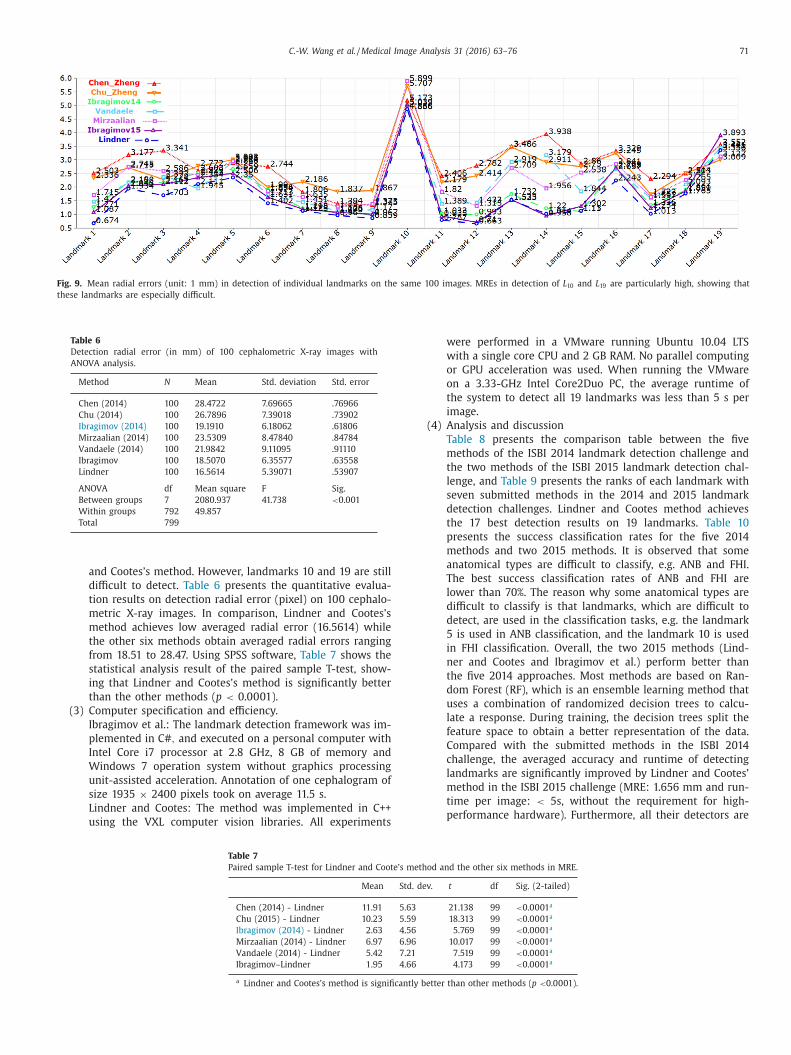
Fig. 9. Mean radial errors (unit: 1 mm) in detection of individual landmarks on the same 100 images. MREs in detection of L 10 and L 19 are particularly high, showing that

these landmarks are especially difficult.

Table 6

Detection radial error (in mm) of 100 cephalometric X-ray images with

ANOVA analysis.

Method N Mean Std. deviation Std. error

Chen (2014) 100 28.4722 7.69665 .76966

Chu (2014) 100 26.7896 7.39018 .73902

Ibragimov (2014) 100 19.1910 6.18062 .61806

Mirzaalian (2014) 100 23.5309 8.47840 .84784

Vandaele (2014) 100 21.9842 9.11095 .91110

Ibragimov 100 18.5070 6.35577 .63558

Lindner 100 16.5614 5.39071 .53907

ANOVA df Mean square F Sig.

Between groups 7 2080.937 41.738 < 0.001

Within groups 792 49.857

Total 799

and Cootes’s method. However, landmarks 10 and 19 are still

difficult to detect. Table 6 presents the quantitative evalua-

tion results on detection radial error (pixel) on 100 cephalo-

metric X-ray images. In comparison, Lindner and Cootes’s

method achieves low averaged radial error (16.5614) while

the other six methods obtain averaged radial errors ranging

from 18.51 to 28.47. Using SPSS software, Table 7 shows the

statistical analysis result of the paired sample T-test, show-

ing that Lindner and Cootes’s method is significantly better

than the other methods ( p < 0.0 0 01).

(3) Computer specification and efficiency.

Ibragimov et al.: The landmark detection framework was im-

plemented in C # , and executed on a personal computer with

Intel Core i7 processor at 2.8 GHz, 8 GB of memory and

Windows 7 operation system without graphics processing

unit-assisted acceleration. Annotation of one cephalogram of

size 1935 × 2400 pixels took on average 11.5 s.

Lindner and Cootes: The method was implemented in C++

using the VXL computer vision libraries. All experiments

Table 7

Paired sample T-test for Lindner and Coote’s me

Mean Std.

Chen (2014) - Lindner 11 .91 5 .63

Chu (2015) - Lindner 10 .23 5 .59

Ibragimov (2014) - Lindner 2 .63 4 .56

Mirzaalian (2014) - Lindner 6 .97 6 .96

Vandaele (2014) - Lindner 5 .42 7 .21

Ibragimov–Lindner 1 .95 4 .66

a Lindner and Cootes’s method is significantly

were performed in a VMware running Ubuntu 10.04 LTS

with a single core CPU and 2 GB RAM. No parallel computing

or GPU acceleration was used. When running the VMware

on a 3.33-GHz Intel Core2Duo PC, the average runtime of

the system to detect all 19 landmarks was less than 5 s per

image.

(4) Analysis and discussion

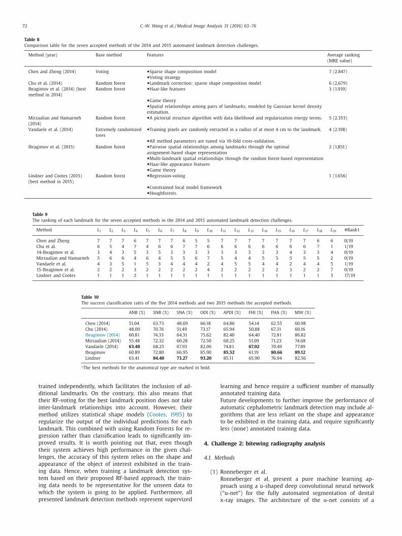
Table 8 presents the comparison table between the five

methods of the ISBI 2014 landmark detection challenge and

the two methods of the ISBI 2015 landmark detection chal-

lenge, and Table 9 presents the ranks of each landmark with

seven submitted methods in the 2014 and 2015 landmark

detection challenges. Lindner and Cootes method achieves

the 17 best detection results on 19 landmarks. Table 10

presents the success classification rates for the five 2014

methods and two 2015 methods. It is observed that some

anatomical types are difficult to classify, e.g. ANB and FHI.

The best success classification rates of ANB and FHI are

lower than 70%. The reason why some anatomical types are

difficult to classify is that landmarks, which are difficult to

detect, are used in the classification tasks, e.g. the landmark

5 is used in ANB classification, and the landmark 10 is used

in FHI classification. Overall, the two 2015 methods (Lind-

ner and Cootes and Ibragimov et al.) perform better than

the five 2014 approaches. Most methods are based on Ran-

dom Forest (RF), which is an ensemble learning method that

uses a combination of randomized decision trees to calcu-

late a response. During training, the decision trees split the

feature space to obtain a better representation of the data.

Compared with the submitted methods in the ISBI 2014

challenge, the averaged accuracy and runtime of detecting

landmarks are significantly improved by Lindner and Cootes’

method in the ISBI 2015 challenge (MRE: 1.656 mm and run-

time per image: < 5s, without the requirement for high-

performance hardware). Furthermore, all their detectors are

thod and the other six methods in MRE.

dev. t df Sig. (2-tailed)

21 .138 99 < 0.0 0 01 a

18 .313 99 < 0.0 0 01 a

5 .769 99 < 0.0 0 01 a

10 .017 99 < 0.0 0 01 a

7 .519 99 < 0.0 0 01 a

4 .173 99 < 0.0 0 01 a

better than other methods ( p < 0.0 0 01).

72 C.-W. Wang et al. / Medical Image Analysis 31 (2016) 63–76

Table 8

Comparison table for the seven accepted methods of the 2014 and 2015 automated landmark detection challenges.

Method (year) Base method Features Average ranking

(MRE value)

Chen and Zheng (2014) Voting •Sparse shape composition model 7 (2.847) •Voting strategy

Chu et al. (2014) Random forest •Landmark correction: sparse shape composition model 6 (2.679)

Ibragimov et al. (2014) (best

method in 2014)

Random forest •Haar-like features 3 (1.919)

•Game theory •Spatial relationships among pairs of landmarks, modeled by Gaussian kernel density

estimation.

Mirzaalian and Hamarneh

(2014)

Random forest •A pictorial structure algorithm with data likelihood and regularization energy terms. 5 (2.353)

Vandaele et al. (2014) Extremely randomized

trees

•Training pixels are randomly extracted in a radius of at most 4 cm to the landmark. 4 (2.198)

•All method parameters are tuned via 10-fold cross-validation.

Ibragimov et al. (2015) Random forest •Pairwise spatial relationships among landmarks through the optimal

assignment-based shape representation

2 (1.851)

•Multi-landmark spatial relationships through the random forest-based representation •Haar-like appearance features •Game theory

Lindner and Cootes (2015)

(best method in 2015)

Random forest •Regression-voting 1 (1.656)

•Constrained local model framework •Houghforests.

Table 9

The ranking of each landmark for the seven accepted methods in the 2014 and 2015 automated landmark detection challenges.

Method L 1 L 2 L 3 L 4 L 5 L 6 L 7 L 8 L 9 L 10 L 11 L 12 L 13 L 14 L 15 L 16 L 17 L 18 L 19 #Rank1

Chen and Zheng 7 7 7 6 7 7 7 6 5 5 7 7 7 7 7 7 7 6 6 0/19

Chu et al. 6 5 4 7 4 6 6 7 7 6 6 6 6 6 6 6 6 7 1 1/19

14-Ibragimov et al. 3 4 3 5 3 5 3 3 3 3 3 3 3 3 3 4 3 3 4 0/19

Mirzaalian and Hamarneh 5 6 6 4 6 4 5 5 6 7 5 4 4 5 5 5 5 5 2 0/19

Vandaele et al. 4 3 5 1 5 3 4 4 4 2 4 5 5 4 4 2 4 4 5 1/19

15-Ibragimov et al. 2 2 2 3 2 2 2 2 2 4 2 2 2 2 2 3 2 2 7 0/19

Lindner and Cootes 1 1 1 2 1 1 1 1 1 1 1 1 1 1 1 1 1 1 3 17/19

Table 10

The success classification rates of the five 2014 methods and two 2015 methods the accepted methods.

ANB (%) SNB (%) SNA (%) ODI (%) APDI (%) FHI (%) FHA (%) MW (%)

Chen (2014) 51.04 63.73 48.69 66.18 64.86 54.14 62.55 60.98

Chu (2014) 48.00 70.76 51.49 73.17 65.94 50.88 67.31 60.16

Ibragimov (2014) 60.81 74.33 64.31 75.62 82.40 64.40 72.81 86.82

Mirzaalian (2014) 55.48 72.32 60.28 72.50 68.25 51.09 71.23 74.68

Vandaele (2014) 63.48 68.25 67.93 82.06 74.81 67.02 70.49 77.89

Ibragimov 60.89 72.80 66.95 85.90 85.52 61.19 80.66 89.12

Lindner 63.41 84.40 73.27 93.20 85.11 65.90 76.94 82.56

∗The best methods for the anatomical type are marked in bold.

4

4

trained independently, which facilitates the inclusion of ad-

ditional landmarks. On the contrary, this also means that

their RF-voting for the best landmark position does not take

inter-landmark relationships into account. However, their

method utilizes statistical shape models ( Cootes, 1995 ) to

regularize the output of the individual predictions for each

landmark. This combined with using Random Forests for re-

gression rather than classification leads to significantly im-

proved results. It is worth pointing out that, even though

their system achieves high performance in the given chal-

lenges, the accuracy of this system relies on the shape and

appearance of the object of interest exhibited in the train-

ing data. Hence, when training a landmark detection sys-

tem based on their proposed RF-based approach, the train-

ing data needs to be representative for the unseen data to

which the system is going to be applied. Furthermore, all

presented landmark detection methods represent supervized

learning and hence require a sufficient number of manually

annotated training data.

Future developments to further improve the performance of

automatic cephalometric landmark detection may include al-

gorithms that are less reliant on the shape and appearance

to be exhibited in the training data, and require significantly

less (none) annotated training data.

. Challenge 2: bitewing radiography analysis

.1. Methods

(1) Ronneberger et al.

Ronneberger et al. present a pure machine learning ap-

proach using a u-shaped deep convolutional neural network

(“u-net”) for the fully automated segmentation of dental

x-ray images. The architecture of the u-net consists of a

C.-W. Wang et al. / Medical Image Analysis 31 (2016) 63–76 73

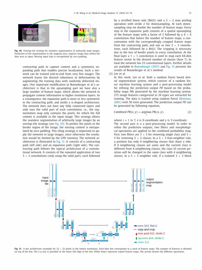
Fig. 10. Overlap-tile strategy for seamless segmentation of arbitrarily large images.

Prediction of the segmentation in the magenta area, requires image data within the

blue area as input. Missing input data is extrapolated by zero padding.

F

o

contracting path to capture context and a symmetric ex-

panding path that enables precise localization. Such a net-

work can be trained end-to-end from very few images. The

network learns the desired robustness to deformations by

augmenting the training data with randomly deformed im-

ages. One important modification in Ronneberger et al.’s ar-

chitecture is that in the upsampling part we have also a

large number of feature maps, which allows the network to

propagate context information to higher resolution layers. As

a consequence, the expansive path is more or less symmetric

to the contracting path, and yields a u-shaped architecture.

The network does not have any fully connected layers and

only uses the valid part of each convolution, i.e., the seg-

mentation map only contains the pixels, for which the full

context is available in the input image. This strategy allows

the seamless segmentation of arbitrarily large images by an

overlap-tile strategy (see Fig. 10 ). To predict the pixels in the

border region of the image, the missing context is extrapo-

lated by zero padding. This tiling strategy is important to ap-

ply the network to large images, since otherwise the resolu-

tion would be limited by the GPU memory. The network ar-

chitecture is illustrated in Fig. 11 . It consists of a contracting

path (left side) and an expansive path (right side). The con-

tracting path follows the typical architecture of a convolu-

tional network. It consists of the repeated application of two

3 × 3 convolutions (only using the valid part), each followed

ig. 11. U-net architecture (example for 32 × 32 pixels in the lowest resolution). Each bl

n top of the box. The x-y-size is provided at the lower left edge of the box. White boxes

by a rectified linear unit (ReLU) and a 2 × 2 max pooling

operation with stride 2 for downsampling. At each down-

sampling step we double the number of feature maps. Every

step in the expansive path consists of a spatial upsampling

of the feature maps with a factor of 2 followed by a 4 × 4

convolution that halves the number of feature maps, a con-

catenation with the correspondingly cropped feature maps

from the contracting path, and one or two 3 × 3 convolu-

tions, each followed by a ReLU. The cropping is necessary

due to the loss of border pixels in every convolution. At the

final layer a 1 × 1 convolution is used to map each 64-dim

feature vector to the desired number of classes (here 7). In

total the network has 23 convolutional layers. Further details

are available in Ronneberger (2015) and Fig. 12 presents the

results of Ronneberger et al.’s method.

(2) Lee et al.

In this work, Lee et al. built a random forest based den-

tal segmentation system, which consists of a random for-

est machine learning system and a post-processing model

for refining the prediction output PD based on the proba-

bility maps PB s generated by the machine learning system.

275 image features categorized in 24 types are extracted for

training. The data is trained using random forest ( Breiman,

2001 ) with 50 trees generated. The prediction output PD can

be generated by following equation.

Combined P B (x, y ) = argmax i

P B i (x, y ) , (2)

where i = 1 to 7, x is X -coordinate and y is Y -coordinate.

The second part is a a post-processing model. In order to

refine the prediction outputs, two filters and morphologi-

cal operations are applied in the combined probability map.

First, two filters are 3 × 3 for removing single class and 5 ×5 for removing 3 × 3 classes. In a 3 × 3 four-neighbor rule,

a position has only 4 neighboring classes that share a side.

If 4 neighboring classes are same and the current class is

different from 4 neighboring classes, the class of current po-

sition will be changed to the same class with 4 neighboring

classes. In a 5 × 5 neighbor rule, if a isolated 3 × 3 block

ue box corresponds to a stack of feature maps. The number of features is denoted

represent copied feature maps. The arrows denote the different operations.

74 C.-W. Wang et al. / Medical Image Analysis 31 (2016) 63–76

Fig. 12. Results of Ronneberger et al.’s method.

Fig. 13. Two filters were used on the probability map in Lee et al.’s method.

with same neighboring classes, all classes of the block will

be changed to the same class with the neighboring classes.

Fig. 13 shows that two filters were used on the probability

map. Fig. 13 (a) is the original combined probability map and

Fig. 13 (b) is the combined probability map after applying 3

× 3 and 5 × 5 filters. Second, the combined PB can be sep-

arated into seven binary prediction maps PDs by following

equations. {P D i (x, y ) = 1 , if Combined P B (x, y ) ∈ i (3) 0 , otherwise (4)

4.2. Quantitative evaluation and analysis

For Challenge 2, all proposed methods are evaluated against the

ground truth on 80 bitewing X-ray images, including 40 Test1 im-

ages and 40 Test2 images.

(1) Quantitative evaluation

Table 11 presents the quantitative evaluation results for the

segmentation of seven dental structures of the two submit-

ted methods. The average precisions of Ronneberger et al.’s

method and Lee et al.’s method are (0.455 and 0.226 in

Test1, 0.419 and 0.195 in Test2), respectively. The best pre-

cisions for segmenting the enamel, dentin, pulp are 0.551,

0.674 and 0.598 in Test1 and 0.542, 0.66 and 0.613 in Test2,

respectively. However, for detecting caries, both methods

perform poor and obtain less than 1% precision. The aver-

aged F-score values of Ronneberger et al.’s method and Lee

et al.’s method are 0.567 and 0.322 in Test1 and 0.525 and

0.287 in Test2.

(2) Computer specification and efficiency

Ronneberger et al.: The network was implemented using the

Caffe-Framework ( Jia, 2014 ), which is written in C++ and

CUDA for the GPU parts. The augmentation and the tiled ex-

ecution are implemented in Matlab. The whole training pro-

cess of one network took about 10 hours on a NVidia Titan

GPU. The execution time is approx. 1.5 sec per image on a

Laptop which was used at the on-site competition (Core i7

CPU, 32 GB RAM, NVidia GTX980m GPU with 8 GB of RAM).

Lee et al.: The algorithm was implemented in Java. In train-

ing phase, all experiments was implemented in a computer

with two Intel Xeon E5-2650 processors at both 2.00 GHz,

128 GB of DDR3 memory and Windows 7 operation system,

and the training phase took about 3.38 hours. In testing step,

all experiments was implemented in a computer with two

Intel Xeon E5-2687 processors at both 3.1 GHz, 16 GB of

DDR3 memory and Windows 7 operation system. The aver-

age execute time is less than 2.5 minutes per bitewing X-ray

image.

(3) Analysis and discussion

Segmentation of dental structures in bitewing radiographs is

difficult as the data variation is high and teeth are some-

times labeled as background (see Fig. 14 ), which makes

the learning task difficult. There are nine teams registered

to this challenge, but only two teams successfully submit-

ted the test results. The averaged F-scores of the teams

C.-W. Wang et al. / Medical Image Analysis 31 (2016) 63–76 75

Table 11

Quantitative evaluation of tooth structure segmentation algorithms on bitewing radiographs.

Test 1 dataset Precision Sensitivity Specificity F-score

Types Ronneberger et al. Lee et al. Ronneberger et al. Lee et al. Ronneberger et al. Lee et al. Ronneberger et al. Lee et al.

Caries 0.073 0.022 0.12 0.06 0.998 0.989 0.119 0.042

Enamel 0.551 0.322 0.685 0.8 0.963 0.746 0.702 0.48

Dentin 0.674 0.48 0.782 0.75 0.936 0.766 0.801 0.642

Pulp 0.598 0.345 0.683 0.573 0.987 0.939 0.74 0.506

Crown 0.295 0.001 0.906 0.024 1 0.982 0.313 0.002

Restoration 0.403 0.241 0.547 0.521 0.996 0.966 0.515 0.349

Root canal treatment 0.179 0.045 0.179 0.144 1 0.999 0.266 0.068

Average 0.455 0.226 0.578 0.548 0.983 0.912 0.567 0.322

Test 2 dataset

Caries 0.078 0.032 0.086 0.05 0.999 0.991 0.131 0.061

Enamel 0.542 0.291 0.736 0.787 0.956 0.753 0.689 0.44

Dentin 0.66 0.44 0.799 0.754 0.933 0.756 0.784 0.601

Pulp 0.613 0.319 0.699 0.608 0.992 0.932 0.748 0.473

Crown 0.295 0.02 0.459 0.205 1 0.99 0.353 0.032

Restoration 0.26 0.145 0.443 0.392 0.992 0.967 0.342 0.23

Root canal treatment 0.098 0.027 0.099 0.058 1 1 0.157 0.045

Average 0.419 0.195 0.531 0.497 0.982 0.913 0.525 0.287

Fig. 14. Six samples of seven dental structures in bitewing radiography with raw image (left side) and manual segmentation result (right side).

5

f

c

s

p

t

c

a

d

d

i

w

d

i

o

o

a

t

r

w

m

(Ronneberger et al. and Lee et al.) are 0.560 and 0.268, re-

spectively, and the u-shaped deep convolutional network by

Ronneberger et al. performs significantly better and achieves

F-scores greater than 0.7 for the three fundamental den-

tal structures ( enamel, dentin and pulp ). The main advantage

of the u-net architecture for this task is its ability to au-

tomatically learn the hierarchical structure within the im-

ages. During segmentation it uses the extracted context at

all detail levels for the decision at each pixel. A critical part

of Ronneberger et al.’s approach is data augmentation. As

there is limited data available, Ronneberger et al. use data

augmentation by applying elastic deformations to produce

a large database with 20 0 0 0 training image tiles, which is

essential for machine learning methods to learn invariance

and produce robust models. The value of data augmenta-

tion for learning invariance has also been shown in Dosovit-

skiy et al. ( Dosovitskiy, 2014 ) in the scope of unsupervised

feature learning. In the experiments, it is observed that the

data augmentation technique helps to create reasonable ad-

ditional training instances for enamel, dentin and pulp, but

the other classes caries, crown, restoration and root canal

treatment, appear quite different according to their relative

location, so the augmentation is less successful here.

. Conclusion

Computerized automatic dental radiography analysis systems

or clinical use save time and manual costs and avoid problems

aused by intra- and inter-observer variations e.g. due to fatigue,

tress or different levels of experience. In this article, we have

resented benchmarks for a number of challenging tasks in den-

al X-ray image analysis, including algorithms for (i) anatomi-

al landmark detection on lateral cephalometric radiographs, (ii)

natomical abnormality classification on lateral cephalometric ra-

iographs, and (iii) dental structure segmentation on bitewing ra-

iographs. The presented results will allow the objective compar-

son of existing and new developments in the field. All methods

ere evaluated using a common lateral cephalometric radiography

ataset repository, a common bitewing radiography dataset repos-

tory, ground truth data, and unified measurements for assessment

f the detection, classification and segmentation accuracy. Based

n the presented results, we can conclude that recent methods

chieved significantly improved performance on these challenging

asks. However, the presented results also demonstrate that accu-

ately analyzing dental radiographs remains a challenging problem

hich is still far from being solved. It is expected that this bench-

ark will help algorithmic developments, and that more advanced

76 C.-W. Wang et al. / Medical Image Analysis 31 (2016) 63–76

L

L

L

L

L

M

N

N

N

O

R

R

R

S

S

T

T

V

W

W

Z

approaches will be built and tested using the provided data repos-

itories and benchmarks.

Acknowledgment

This work was supported by Tri-Service General Hospital-

National Taiwan University of Science and Technology (TSGH-

NTUST-C104011008 and C103008), Taiwan Ministry of Science and

Technology ( MOST1042221E011085 ) and Cardinal Tien Hospital

(CTH10212C02). Ibragimov et al. was supported by the Slovenian

Research Agency ( P2-0232, L2-4072, J2-5473 and J7-6781 ). C. Lind-

ner is funded by the Engineering and Physical Sciences Research

Council , UK ( EP/M012611/1 ). Ronneberger et al. was supported by

the Excellence Initiative of the German Federal and State govern-

ments (EXC294) and by the BMBF (Fkz0316185B).

References

Breiman, L. , 2001. Random forests. Mach. Learn. 45, 5–32 .

Cootes, T. , 1995. Active shape models - their training and application. Comput. Vis.Image Und. 61, 38–59 .

Dosovitskiy, A. , 2014. Discriminative unsupervised feature learning with convolu-tional neural networks. In: NIPS .

Downs, W.B. , 1948. Variations in facial relationship, their significance in treatment

and prognosis. Am. J. Orthod. 34 (10), 812–840 . Gayathri, V. , Menon, H.P. , 2014. Challenges in edge extraction of dental x-ray images

using image processing algorithms - a review. Int. J. Comput. Sci. Inf. Technol.5, 5355–5358 .

Huh, J. , 2015. Studies of automatic dental cavity detection system as an auxiliarytool for diagnosis of dental caries in digital x-ray image. Progr. Med. Phys. 25,

52–58 .

Ibragimov, B. , 2012. A game-theoretic framework for landmark-based image seg-mentation. IEEE Trans. Med. Imag. 31 (9), 1761–1776 .

Ibragimov, B. , 2014. Shape representation for efficient landmark-based segmentationin 3d. IEEE Trans. Med. Imag. 33 (4), 861–874 .

Ibragimov, B. , 2015. Segmentation of tongue muscles from super-resolution mag-netic resonance images. Med. Image Anal. 20 (1), 198–207 .

Jain, A.K. , Chen, H. , 2004. Matching of dental x-ray images for human identification.

Pattern Recognit. 37, 1519–1532 . Jia, Y. , 2014. Caffe: convolutional architecture for fast feature embedding. Proc. ACM

Int. Conf. Multimed. 675–678 . Kim, Y.H. , 1974. Overbite depth indicator: with particular reference to anterior open-

bite. Am. J. Orthod. 65 (6), 586–611 . Kim, Y.H. , Vietas, J.J. , 1978. Anteroposterior dysplasia indicator: an adjunct to

cephalometric differential diagnosis. Am. J. Orthod. 73 (6), 619–633 . Kumar , 2011. Extraoral periapical radiography: an alternative approach to intraoral

periapical radiography. Imag. Sci. Dent. 41, 161–165 .

ai, Y.H. , Lin, P.L. , 2008. Effective segmentation for dental x-ray images using tex-ture-based fuzzy inference system. Adv. Concepts Intell. Vis. Syst. Lect. Notes

Comput. Sci. 5259, 936–947 . in, P.L. , 2010. An effective classification and numbering system for dental bitewing

radiographs using teeth region and contour information. Pattern Recognit. 43,1380–1392 .

indner, C. , et al. , 2013. Fully automatic segmentation of the proximal femur usingrandom forest regression voting. IEEE Trans. Med. Imag. 32, 1462–1472 .

indner, C. , et al. , 2015. Robust and accurate shape model matching using random

forest regression-voting. IEEE Trans. Pattern Anal. Mach. Intell. 37, 1862–1874 . pez-Lpez, J. , 2012. Computer-aided system for morphometric mandibular index

computation (using dental panoramic radiographs). Med. Oral Patol. Oral 17,e624–e632 .

cNamara, J.J. , 1984. A method of cephalometric evaluation. Am. J. Orthod. 86 (6),449–469 .

akamoto, T. , 2008. A computer-aided diagnosis system to screen for osteoporosis

using dental panoramic radiographs. Dentomaxillofacial Radiol. 37, 274–281 . anda, R. , Nanda, R.S. , 1969. Cephalometric study of the dentofacial complex of

north indians. Angl. Orthod. 39 (1), 22–28 . ikneshan, S. , 2015. The effect of emboss enhancement on reliability of landmark

identification in digital lateral cephalometric images. Iran. J. Radiol. 12, e19302 . liveira, J. , Proenc, H. , 2011. Caries detection in panoramic dental x-ray images.

Comput. Vis. Med. Image Process.: Recent Trends, Comput. Meth. Appl. Sci. 19,

175–190 . ad, A.E. , 2013. Digital dental X-ray image segmentation and feature extraction.

TELKOMNIKA 11, 3109–3114 . icketts, R.M. , et al. , 1982. Orthodontic Diagnosis and Planning, I and II. Rocky

Mountain Orthod, Denver . onneberger, O., 2015. U-net: Convolutional networks for biomedical image seg-

mentation. In: Medical Image Computing and Computer-Assisted Intervention

(MICCAI) . accepted, url = http://arxiv.org/abs/1505.04597. assouni, V. , 1955. A roentgenographic cephalometric analysis of cephalo-facio-den-

tal relationships. Am. J. Orthod. 41, 735–764 . 1955 teiner, C.C. , 1953. Cephalometrics for you and me. Am. J. Orthod. 39 (10), 729–755 .

weed, C. , 1946. The frankfort-mandibular plane angle in orthodontic diagnosis,classification, treatment planning, and prognosis. Am. J. Orthod. Oral Surg. 32

(1), 175–230 .

weed, C.H. , 1954. The frankfort mandibular incisal angle (FMIA) in orthodontic di-agnosis, treatment planning, and prognosis. Angl. Orthod. 24, 121–169 .

iola, P. , Jones, M. , 2001. Rapid object detection using a boosted cascade of simplefeatures. In: Proceedings CVPR 2001, pp. 511–518 .

ang, C.W. , 2015. Evaluation and comparison of anatomical landmark detectionmethods for cephalometric X-ray images: A grand challenge. IEEE Trans. Med.

Imag. 34 (9), 1–11 .

Wenzel, A. , 2001. Computer-automated caries detection in digital bitewings: consis-tency of a program and its influence on observer agreement. Caries Res. 35 (1),

12–20 . enzel, A. , et al. , 2002. Accuracy of computer-automated caries detection in digital

radiographs compared with human observers. Eur. J. Oral Sci. 110 (3), 199–203 . Wriedt, S. , 2012. Impacted upper canines: examination and treatment proposal

based on 3d versus 2d diagnosis. J. Orofac. Orthop. 73, 28–40 . hou, J. , Abdel-Mottaleb, M. , 2005. A content-based system for human identification

based on bitewing dental X-ray images. Pattern Recognit. 38, 2132–2142 .