Journal of

Mechanics ofMaterials and Structures

MECHANICS OF MATERIALS AND STRUCTURES:A SIMULATION-DRIVEN DESIGN APPROACH

Lennart Karlsson, Andreas Pahkamaa, Magnus Karlberg, Magnus Löfstrand, John Goldakand Jonas Pavasson

Volume 6, No. 1-4 January–June 2011

mathematical sciences publishers

JOURNAL OF MECHANICS OF MATERIALS AND STRUCTURESVol. 6, No. 1-4, 2011

msp

MECHANICS OF MATERIALS AND STRUCTURES:A SIMULATION-DRIVEN DESIGN APPROACH

LENNART KARLSSON, ANDREAS PAHKAMAA, MAGNUS KARLBERG,MAGNUS LÖFSTRAND, JOHN GOLDAK AND JONAS PAVASSON

Engineering product development has developed considerably over the past decade. In order for industryto keep up with continuously changing requirements, it is necessary to develop new and innovativesimulation methods. However, few tools and methods for simulation-driven design have been applied inindustrial settings and proven to actually drive the development and selection of the ideal solution. Suchtools, based on fundamental equations, are the focus of this paper.

In this paper the work is based on two cases of mechanics of materials and structures: welding androtor dynamical simulations. These two examples of simulation-driven design indicate that a largerdesign space can be explored and that more possible solutions can be evaluated. Therefore, the approachimproves the probability of innovations and finding optimal solutions.

A calibrated block dumping approach can be used to increase the efficiency of welding simulationswhen many simulations are required.

1. Introduction

Engineering product development has evolved considerably over the past decade. The vision of thesustainable society and a global context for many industries is now forcing manufacturing companiesto develop innovative ways of developing their products. In addition, the product life-cycle will likelybe shorter in the future, partly because customers will demand shorter delivery times. Suppliers willhave to be more efficient than today and be able to assemble products from a large number of partsfrom subsuppliers. Increasingly, the value of the product originates outside the physical artifact (thehardware), in the form of services and add-ons. Instead of hardware ownership, other needs such asavailability, productivity and risk minimization increasingly need to be catered for. In such a challengingenvironment and in order for industry to keep up with demand, it is necessary to develop new andinnovative simulation methods, knowledge management methods and tools and methods for distributedwork, to name a few.

In this paper, the focus is mainly on simulation-driven design applied on welding simulations (me-chanics of materials) and rotor dynamical design (mechanics of structures). Below, the basic equationsfor modeling and simulation of welding and the basic equations for modeling and simulation of nonlineardynamics are solved. For these two important problems, the way in which this fundamental modelingcan effectively be used in simulation-driven product development is demonstrated.

Keywords: simulation-driven design, calibrated block dumping, welding simulations, rotor dynamical simulations.

277

278 L. KARLSSON, A. PAHKAMAA, M. KARLBERG, M. LÖFSTRAND, J. GOLDAK AND J. PAVASSON

Planning // Conceptdevelopment

// System-leveldesign

// Detaildesign

// Testing andrefinement

// Productionramp-up

Figure 1. An example of a product development process.

Most industrial companies of any size follow some development process when developing their prod-ucts. Figure 1 shows an example of such a development process from planning to production ramp-up[Ulrich and Eppinger 1995].

Product development literature provides a broad view of how to understand customer needs, developand sell products, and includes discussions concerning best practices [Ulrich and Eppinger 1995; Wheel-wright and Clark 1992; Cross 2000]. For example, Smith and Reinertsen [1998] offer a general view andaim to describe methods for generating a product to meet customer needs. Recently, product developmentprocesses have been extended to cover the whole process from needs to recycling.

Within the hardware product development domain, numerous tools have been developed to supportthe creation of excellent goods; e.g., computer aided engineering for geometric representation [LaCourse1995] and the finite element method for stress calculation, exemplified in this paper. Typically, thiswork has been about making knowledge explicit and expressible and support tools have over time beendeveloped to aid the creation of the hardware.

Simulations are ideally supposed to be used in the earliest stages of the development process. Often,however, there are few analyses involved until the detailed design stage is reached. At this stage simula-tions are often used in a verifying sense, meaning that the designer submits a model to the analysts whoperform the analysis and then deliver the results to the designer. The results are used by the designer toverify whether or not the proposed design will meet the criteria. If not, the designer needs to upgradethe initial design, and then propose a new design for the analysts who perform a new simulation and soon, see Figure 2.

This sequential simulation usage workflow in combination with little usage of simulations in the earli-est stages of the development process gives an ineffective product development process. To overcome thisproblem strategies for simulation-driven development have been proposed by some researchers [Courter2009; Sellgren 1995; Wall 2007]. Naturally, such work has been ongoing for a relatively long time, asexemplified by [Hansen 1974] and [Gero 1981]. The development processes discussed in literature areoften analyzed from an abstract point of view, while few reports exist on how simulation tools shall bedesigned and used to enable such methodologies. That is, few tools and methods have been applied inindustrial settings and proven to actually drive the development and selection of the ideal solution.

Given these challenges, this paper is focused on briefly introducing the area of simulation drivendesign (SDD) [Courter 2009], and based on that approach describing a block dumping technique appliedin welding simulations. Another application of the SDD approach is presented in the application area ofrotor dynamical design.

Proposeddetailed design

// Analysis // Redesign // Analysis // Redesign

Figure 2. Sequential verifying simulation usage workflow.

MECHANICS OF MATERIALS AND STRUCTURES: A SIMULATION-DRIVEN DESIGN APPROACH 279

Thus, the objective of this paper is to show how tools for modeling and simulation of mechanics ofmaterials and structures shall be designed and used to enable simulation-driven product development.The objective is exemplified through two cases of mechanics of materials and structures: welding androtor dynamical simulations.

2. Simulation-driven design methodology

In this paper a simulation-driven methodology is used [Bylund 2004; Goldak et al. 2007]. Bylund statesthat one way of reaching simulation-driven design is by providing simulation tools that can be used bythe designers themselves. Designers thereby avoid having to send models and results back and forth,often among several different people. For designers not used to analysis work to be able to perform thenecessary analyses, tools that are intuitive and include expert knowledge through equations of mechanicsof materials and structures are required. The results from the analyses must further be derived quicklyand must be easy to interpret. Hence, the demands on the simulation tools affect the preprocessing, thesolver and the postprocessing.

3. Simulation-driven design of welded structures

Welding is one of the most commonly used methods of joining metal pieces. In fusion welding, themetal pieces are heated until they melt together, resulting in strong coupling between thermal, mechan-ical and metallurgical (microstructural) properties. Due to the complexity of the welding applications,the governing equations as well as the thermal, mechanical and metallurgical couplings, computationalsupport is necessary for prediction of distortions and residual stresses. The development of the fieldof computational welding mechanics has been described in, for example, [Karlsson 1986; Goldak andAkhlaghi 2005; Lindgren 2001a; 2001b; 2001c; 2007]. Much research has focused on predictions ofresidual stresses and distortions [Chen and Sheng 1992; Lee et al. 2008; Ueda et al. 1988; Ueda andYuan 1993].

Several reports exist regarding validation of predictions of residual stresses and deformation [Barrosoet al. 2010; Karlsson et al. 1989; Mochizuki et al. 2000; Ueda et al. 1986]. The European Networkon Neutron Techniques Standardization for Structural Integrity (NeT) has a benchmark problem for asingle weld bead-on-plate specimen [Truman and Smith 2009]. By using finite element simulations, NeTmembers have predicted and measured residual stresses and thermal fields of this benchmark problem bydifferent methods, the results of which have been compiled [Smith and Smith 2009a; 2009b]. In thosereports, different sources of errors are discussed, and it was also found that “there is much room forimprovement” regarding prediction accuracy.

In product development, residual stresses and distortions often need predicting to verify alignmenttolerances, strength demands, fatigue requirements, etc. It is important, for example, to keep track of theresidual stress- and deformation history when simulating a sequence of manufacturing processes [Denget al. 2009; Åström 2004]. Different approaches have been developed for how to use welding simulationsto predict suitable sequences of weld paths. Troive et al. [1998] compared different predefined paths,while Voutchkov et al. [2005] used surrogate models to solve a combinatorial weld path planning problem.Efforts have further been made to show effects of deposition sequences regarding, for instance, residualstresses and distortions [Ogawa et al. 2009]. Although a lot of research has been conducted on welding

280 L. KARLSSON, A. PAHKAMAA, M. KARLBERG, M. LÖFSTRAND, J. GOLDAK AND J. PAVASSON

simulations, there is still a need for development of more efficient welding simulations and methodologiesfor using such simulations to support design processes.

In this article, a strategy for improved efficiency of welding simulations is used as proposed in [Pahka-maa et al. 2010], aiming at developing a simulation-driven design methodology for welding simulations.In this work, the modeling and simulation software VrWeld from Goldak Technologies Inc. [GoldakTechnologies 2010] has been used to demonstrate the proposed strategy.

3.1. Welding simulation theory. The field of welding simulations described in this paper (computationalwelding mechanics) is partially built upon earlier work within the fields of thermal, mechanical and metal-lurgical (microstructural) properties of materials. The principles and applications of welding simulationshave been described in [Goldak and Akhlaghi 2005; Lindgren 2001b]. Welding simulation is a goodexample of how mechanics of materials and structures can be put to practical use with the support ofcomputers. The essential features of computational weld mechanics (CWM) are [Goldak 2009]:

• It requires solving the nonlinear, coupled 3D transient partial differential equations (PDEs) for heatflow (conservation of energy), microstructure evolution and stress-strain evolution (conservation ofmomentum).

• The material properties are temperature, history dependent and involve phase changes.

• The welding process usually adds material (filler metal), making the geometric domain a time-dependent free surface problem.

• The boundary conditions applied by fixtures, clamps and tack welds are complex and transient.

• The geometry of welded structures is often complex with many parts.

• Modeling the heat source of the arc is itself complex.

3.1.1. Welding simulation software (VrWeld). VrWeld, part of the VrSuite software package, is a finiteelement program used to simulate welding processes. VrSuite [Goldak Technologies 2010] uses operatorsplitting to solve the system of equations needed to model manufacturing processes such as welding andheat treating and the in-service behavior of assemblies of such manufactured parts. Each equation inthe system is solved with the algorithm, domain, parameters, initial conditions, boundary conditions,length scale and time scale that best approximate the physics of the phenomena that the equation models.Maps are created to map data from this equation to each equation that it is coupled to. Each equationis solved iteratively using solvers such as frontal, multifrontal, ICCG, GMRES, MG and AMG [Saad1996]. Limits and bifurcation points are computed using the Wriggers–Simo algorithm [Wriggers andSimo 1990]. A version of Crisfield’s arc-length method [Ramm 1981] is used to follow the path of thesolution in nonlinear analysis. The meshing is largely automated. Domain decomposition and adaptivemeshing play an important role. Solvers run in-core using processors with 8 GB of RAM. The CPU-intensive code is written in C++. The high-level code is written in a scripting language such as Tcl/Tkor HTML.

3.1.2. Block dumping (fast simulations in VrWeld). Traditional transient welding simulations often usea moving heat source such as the Gaussian double ellipsoid [Goldak and Akhlaghi 2005]; see Figure 3.This approach has proved to accurately predict the temperature history, residual stresses and weldingdistortions [Goldak and Akhlaghi 2005; Lindgren 2001a; 2001b; 2001c; 2007]. It is suggested that the

MECHANICS OF MATERIALS AND STRUCTURES: A SIMULATION-DRIVEN DESIGN APPROACH 281

Figure 3. Double ellipsoid heat source with Gaussian heat distribution [Goldak andAkhlaghi 2005].

heat source may move no more than half of the weld pool length to function properly in three dimensionalwelding simulations [Goldak et al. 1986]. This suggestion causes a transient welding simulation thatuses a moving heat source to be quite time consuming, even with present-day computational power.The problem gets even more difficult when a large design space is to be explored, meaning that manysimulations are required.

A faster way to simulate the thermal history of a weld is the block dumping method [Goldak et al.1986], also referred to as the prolonged Gaussian heat source [Cai and Zhao 2003]. The block dumpingapproach heats the whole weld, or large pieces of it, in a single time step. This approach can reducethe number of time steps in the welding simulation significantly and thereby reduce the total calculationtime without any appreciable decrease in accuracy [Pahkamaa et al. 2010]. With the block dumpingtechnique, the same parameters as the Gaussian Ellipsoid heat source are used to calculate the amountof heat distributed to each element, i.e., voltage, current, efficiency, welding speed and parameters a1,a2, b and c in Figure 3. The total amount of heat distributed to the model is identical to the heat inputof a traditional transient simulation. The difference is the time in which the heat is diffused. In eachblock dump, the amount of heat added is exactly the same as the heat that would be added in a transientanalysis for this length of weld, and it is added in exactly the same way with the same transient time steps.However, no heat diffusion is done until all heat has been added for this length of weld. Then one heatingtime step is done with these applied nodal thermal loads to heat this length of weld. Following this heatingtime step, the heat equation is solved for the structure as it cools with exponentially increasing length oftime steps. Usually, 4 to 6 cooling time steps are applied. The designer can choose to allow each blockdump to cool to ambient temperature or use a shorter cooling time in which the structure does not fullycool, the latter approach is used in this paper. In the heating and cooling steps, the thermal-elastoplasticstress analysis problem is solved. This process is applied for each block dump in the sequence of blockdumps specified by the designer.

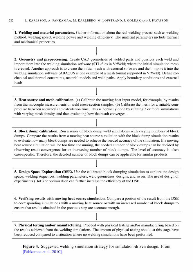
3.2. Simulation strategy. The welding simulation strategy proposed in [Pahkamaa et al. 2010] (Figure 4),which will be verified in this study, reduces the calculation time for welding simulations by replacing thetraditional moving heat source with a calibrated block dumping heat source. The block dumping heat

282 L. KARLSSON, A. PAHKAMAA, M. KARLBERG, M. LÖFSTRAND, J. GOLDAK AND J. PAVASSON

1. Welding and material parameters. Gather information about the real welding process such as weldingmethod, welding speed, welding power and welding efficiency. The material parameters include thermaland mechanical properties.

2. Geometry and preprocessing. Create CAD geometries of welded parts and possibly each weld andimport them into the welding simulation software (STL-files in VrWeld) where the initial simulation meshis created. Another approach is to create the initial mesh with external software and then import it into thewelding simulation software (ABAQUS is one example of a mesh format supported in VrWeld). Define me-chanical and thermal constraints, material models and weld paths. Apply boundary conditions and externalloads.

3. Heat source and mesh calibration. (a) Calibrate the moving heat input model, for example, by resultsfrom thermocouple measurements or weld cross-section samples. (b) Calibrate the mesh for a suitable com-promise between accuracy and calculation time. This is normally done by running 3 or more simulationswith varying mesh density, and then evaluating how the result converges.

4. Block dump calibration. Run a series of block dump weld simulations with varying numbers of blockdumps. Compare the results from a moving heat source simulation with the block dump simulation resultsto evaluate how many block dumps are needed to achieve the needed accuracy of the simulation. If a movingheat source simulation will be too time consuming, the needed number of block dumps can be decided byobserving result convergence for an increasing number of block dumps. The level of accuracy is oftencase-specific. Therefore, the decided number of block dumps can be applicable for similar products.

5. Design Space Exploration (DSE). Use the calibrated block dumping simulation to explore the designspace: welding sequences, welding parameters, weld geometries, designs, and so on. The use of design ofexperiments (DoE) or optimization can further increase the efficiency of the DSE.

6. Verifying results with moving heat source simulation. Compare a portion of the result from the DSEto corresponding simulations with a moving heat source or with an increased number of block dumps toensure that results obtained in the previous step are accurate enough.

7. Physical testing and/or manufacturing. Proceed with physical testing and/or manufacturing based onthe results achieved from the welding simulations. The amount of physical testing should at this stage havebeen reduced compared to a situation where no welding simulations have been performed.

Figure 4. Suggested welding simulation strategy for simulation-driven design. From[Pahkamaa et al. 2010].

MECHANICS OF MATERIALS AND STRUCTURES: A SIMULATION-DRIVEN DESIGN APPROACH 283

Figure 5. Rear frame and rear axle bridge.

source is calibrated to give a good compromise between simulation accuracy and calculation time, thusallowing a larger design space to be explored during a given period of time. A rear axle bridge froma Volvo Construction Equipment wheel loader is used as a demonstrator case to show that steps 1–6work on an industrial application. Twenty different welding sequences are compared to find the weldingsequence that gives the smallest welding distortion at key positions.

3.3. Welding case study. The object of this case study is a rear axle bridge from a Volvo ConstructionEquipment wheel loader. The axle bridge is positioned in the rear frame as in Figure 5. An axle workingas a pivot for the rear axle assembly is mounted in the two holes in the axle bridge. The axle is supportedby journal bearings, which are lubricated with oil from the rear axle differential. The concentricitybetween the two holes and the parallelism and perpendicular alignment between the plates are two im-portant tolerance demands for the axle bridge. Due to these requirements, it is important that the weldingprocess used to manufacture the axle bridge does not introduce excessive deformations. Therefore, theaim of this case study is to derive a suitable welding sequence that minimizes the welding distortion inthe axle bridge. Identifying the proper welding sequences is done by use of the proposed simulationstrategy; see Figure 4.

3.3.1. Welding and material properties. The three plates are joined by welds, marked a–d in Figure 6;the welds have a throat size of 6 mm. The axle bridge is manually tack-welded with 40 mm long tackwelds at start, mid and end of the four welds. The tack welding is performed in a separate fixture; thetack welded axle bridge is then positioned in the welding fixture shown in Figure 6. An automated MAGwelding process then applies the four welds, with the following parameters:

Power : 10880 W (34 V, 320 A)Efficiency : 85%

Welding speed : 37 cm/min

3.3.2. Geometry and preprocessing. A CAD model of the axle bridge assembly was provided by themanufacturer. This CAD model was imported to Siemens PLM NX6, where small features were re-moved to ease the meshing process. The idealized part shown in Figure 7 was exported to the welding

284 L. KARLSSON, A. PAHKAMAA, M. KARLBERG, M. LÖFSTRAND, J. GOLDAK AND J. PAVASSON

Figure 6. Real axle bridge placed in its welding fixture. The weld joints (a–d) aremarked with white lines; welds a and c are placed underneath the center plate.

simulation software (VrWeld) in STL-format. The simulation model was then created in VrWeld bydefining weld joints, assigning materials, creating an initial mesh and assigning initial conditions andboundary conditions, etc. The material model described in [Andersson 1978] was used for both platesand filler metal. The used fixture shown in Figure 7 prevents rigid body motions (locks six DOFs)without restraining the growth/shrinkage of the plates. This fixture modeling method was used, since thereal fixture only clamps one of the plates, and should therefore not have a large impact on the weldingdistortions. The welding distortion in the rear axle bridge was measured as the global displacement ofpoints P1 and P2. The global ambient temperature is set to 300 K.

Figure 7. Idealized axle bridge, evaluation points and constraints.

MECHANICS OF MATERIALS AND STRUCTURES: A SIMULATION-DRIVEN DESIGN APPROACH 285

Figure 8. Comparison of weld cross section photograph and simulated heat input.

3.3.3. Moving heat input calibration. The moving heat input model was calibrated by use of a weldcross section photograph, see Figure 8. The trial and error method was used to find suitable heat inputparameters that describe the shape of the Double Ellipsoid heat source. The calibrated parameters are asfollows (see Figure 3):

a1 = 10 mm a2 = 6 mm b = 6 mm c = 8 mm

3.3.4. Mesh and block dump calibration. Three models with different mesh density were created, asfollows:

Mesh # Volume elements Elements in weld joint (cross-section)1 13237 52 27142 7–93 42665 12–15

For each of them, seven welding simulations were run, with an increasing number of block dumps (4,8, 15, 20, 30, 40, 50). Ten cooling time steps were used in each block dump simulation. The “FastSimulation” option in VrWeld uses the same number of block dumps for all welds. Therefore, a full-length weld will be welded with the same number of block dumps as a half-length weld. Thus, a weldingsequence with full-length welds and, for example, 20 block dumps will be simulated in 90 time steps(4 welds × 20 block dumps + 10 cooling time steps), while a welding sequence with half-length weldswill be simulated in 170 time steps (8 welds × 20 block dumps + 10 cooling time steps). The case usedto calibrate the mesh and number of block dumps has four half-length welds and two full-length welds(see Appendix).

The absolute displacement of points P1 and P2 (see Figure 7) was used to evaluate the results. Figure 9shows results for point P1, similar results were obtained for point P2. From Figure 9 it can be concludedthat there is little difference in results between mesh 2 and 3, while the results from mesh 1 deviatesignificantly. The difference between mesh 2 and 3 is only 0.1 mm when 40 block dumps are used. Basedon these results, mesh number 2 and 40 block dumps will be used for the DSE. The chosen simulation

286 L. KARLSSON, A. PAHKAMAA, M. KARLBERG, M. LÖFSTRAND, J. GOLDAK AND J. PAVASSON

4 8 15 20 30 40 500

2

4

6

8

10

Block Dumps

Dis

pla

cem

ent [m

m]

Absolute displacement P1

Mesh 1Mesh 2Mesh 3

Figure 9. Mesh and block dump calibration. There is a difference of 0.1 mm betweenMesh 2 and Mesh 3 when 40 block dumps are used.

Figure 10. The chosen simulation mesh has 8 elements across the weld joint and 27142elements in total.

mesh is shown in Figure 10. To verify predictions made by use of the chosen mesh and number of blockdumps, the results should be compared with the results from simulations with a moving heat source. Ifthe same best welding sequence is being predicted by the two models, the chosen mesh and number ofblock dumps are considered to be sufficient.

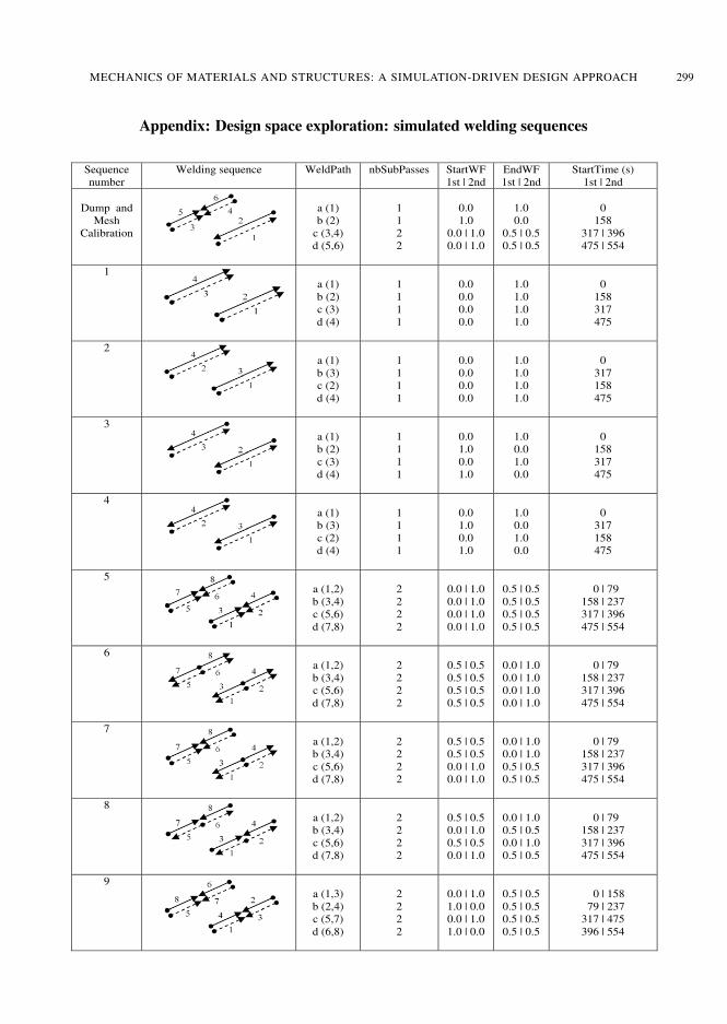
3.3.5. Design space exploration. A structure that has four welds, such as the axle bridge, can be weldedin 384 (24

× 4!) different ways. The large number of combinations is possible when allowing the weldsto be laid in any order (4!) and in both directions (24). If only half welds are allowed, the number ofpossible welding combinations grows to about 10 million possible combinations (28

× 8!). Design spaceexploration (DSE) refers to exploring the set of possible welding combinations and selecting a subsetwhich meets the requirements. In this case, it is not practical to explore the entire design space. Toshow how welding sequences influence the displacements in P1 and P2, twenty different sequences are

MECHANICS OF MATERIALS AND STRUCTURES: A SIMULATION-DRIVEN DESIGN APPROACH 287

0 2 4 6 8 10 12 14 16 18 20−10

−5

0

5

10Displacement P1

Sequence number

Dis

pla

ce

me

nt

[mm

]

xyzabs

0 2 4 6 8 10 12 14 16 18 20−10

−5

0

5

10Displacement P2

Sequence number

Dis

pla

ce

me

nt

[mm

]

xyzabs

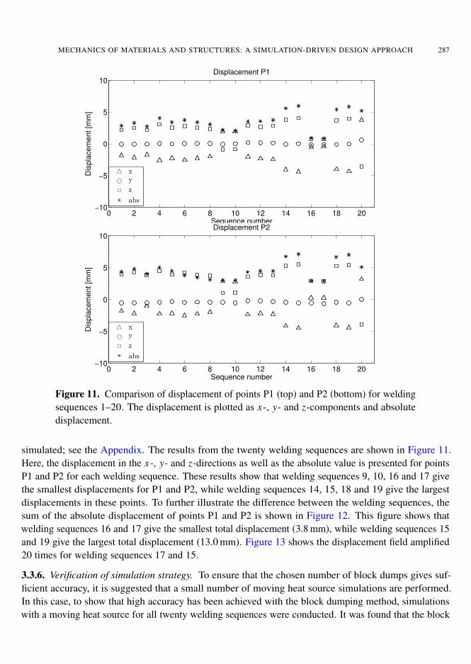
Figure 11. Comparison of displacement of points P1 (top) and P2 (bottom) for weldingsequences 1–20. The displacement is plotted as x-, y- and z-components and absolutedisplacement.

simulated; see the Appendix. The results from the twenty welding sequences are shown in Figure 11.Here, the displacement in the x-, y- and z-directions as well as the absolute value is presented for pointsP1 and P2 for each welding sequence. These results show that welding sequences 9, 10, 16 and 17 givethe smallest displacements for P1 and P2, while welding sequences 14, 15, 18 and 19 give the largestdisplacements in these points. To further illustrate the difference between the welding sequences, thesum of the absolute displacement of points P1 and P2 is shown in Figure 12. This figure shows thatwelding sequences 16 and 17 give the smallest total displacement (3.8 mm), while welding sequences 15and 19 give the largest total displacement (13.0 mm). Figure 13 shows the displacement field amplified20 times for welding sequences 17 and 15.

3.3.6. Verification of simulation strategy. To ensure that the chosen number of block dumps gives suf-ficient accuracy, it is suggested that a small number of moving heat source simulations are performed.In this case, to show that high accuracy has been achieved with the block dumping method, simulationswith a moving heat source for all twenty welding sequences were conducted. It was found that the block

288 L. KARLSSON, A. PAHKAMAA, M. KARLBERG, M. LÖFSTRAND, J. GOLDAK AND J. PAVASSON

0 2 4 6 8 10 12 14 16 18 200

5

10

15

20

Sequence number

Dis

pla

ce

me

nt

[mm

]

Total displacement (P1+P2)

40 Dumps

Figure 12. Total displacement calculated as the sum of the absolute displacement ofpoints P1 and P2. Notice that welding sequences 16 and 17 give the smallest total dis-placement (4 mm), while welding sequences 15 and 19 give the largest total displacement(13 mm).

Figure 13. Comparison of best (#17) and worst (#15) welding sequences. Colors indi-cate displacements, given in mm on the scale on the right and magnified 20 times in thegeometric representation.

dumped simulations deviate by 0.7 mm (mean value) compared to the moving heat source simulations.Both simulation approaches predict the same welding sequences to give the smallest and largest weldingdistortions in P1 and P2. Welding sequences 1–4 are welded with full-length welds only and simulatedin 170 time steps. Welding sequence 20 is welded with two full-length welds and four half-length weldsand simulated in 250 time steps. Welding sequences 5–19 are welded with eight half-length welds andsimulated in 330 time steps. The moving heat source is simulated in 450 time steps. Hence, the numberof time steps has then been reduced by 60% (welding sequences 1–4), 45% (welding sequence 20) and25% (welding sequences 5–19).

3.4. Welding case discussion. This case study has shown that calibrated block dumping simulationscan reduce the calculation time compared to moving heat source simulations. The results from the block

MECHANICS OF MATERIALS AND STRUCTURES: A SIMULATION-DRIVEN DESIGN APPROACH 289

0 2 4 6 8 10 12 14 16 18 200

5

10

15

20

Sequence number

Dis

pla

ce

me

nt

[mm

]

Total displacement (P1+P2)

40 DumpsMoving

Figure 14. Comparison between block dumped and moving heat source simulations.

dumped simulations were able to point out the best (16 and 17) and worst (15 and 19) welding sequences(Figure 14), which was identical to the results obtained with the moving heat source simulations. Theblock dump calibration and mesh calibration for this case study was performed by running 21 simulations.Thus, using the calibrated block dump method to simulate as few as twenty welding sequences will notsave much time. The strength of this method becomes obvious when a larger design space is explored,when hundreds or thousands of welding simulations are performed.

This work is done on the assumption that the 3D transient welding simulations approach used in thispaper is able to predict residual stresses and welding distortions correctly. Future work should involvevalidation of the simulation results obtained in this paper.

This case study has shown that it should be possible to use a simulation-driven design approach inthe design process regarding welded structures. Twenty different welding sequences were compared,showing that welding sequences 16 and 17 gave the smallest welding distortions in P1 and P2 and couldtherefore be considered as the best suited for this structure.

Future work should explore the possibilities of combining the calibrated block dumping simulationswith design of experiments or optimization routines to further rationalize the design process of weldedstructures. A computer program made to generate suitable welding sequences to be explored wouldsignificantly decrease designer manual labor. The welding sequences listed in Table 2 where definedmanually, which was a quite time consuming task.

It would also be valuable to perform a similar case study where the block dumps are defined by theirlength instead of the number of block dumps per weld.

4. Simulation-driven rotor dynamical design

Few CAE systems support rotor dynamical analysis, and if they do they have restricted functionality.Therefore, specialized software is commonly used when designing rotating machinery. These specializedrotor dynamical codes often include a lot of functionality, but for nonexperts, they can be difficult to use.In order to facilitate simulation-driven design, an in-house rigid body rotor dynamical demonstrator code

290 L. KARLSSON, A. PAHKAMAA, M. KARLBERG, M. LÖFSTRAND, J. GOLDAK AND J. PAVASSON

called RESORS has been developed at Luleå University of Technology, Division of Computer AidedDesign. The aim is to enable nonexperts to conduct advanced nonlinear rotor dynamical analyses veryearly in the product development process. By this strategy, sending analysis requests to experts can beavoided, allowing possibilities for exploring a larger part of the design space.

4.1. Rotor dynamical theory. Rotor dynamical theory was basically developed during the last century,but started earlier, with Rankine [1869], who incorrectly predicted that the first critical speed could notbe exceeded. In the late nineteenth century, de Laval practically proved (see [Childs 1993]) that rotatingmachinery can run supercritically, which was later verified by Jeffcott [1919]. Since it was introduced, theJeffcott rotor model has been widely used for different scientific purposes; see for example [Childs 1982;Karlberg and Aidanpää 2003; Karlberg and Aidanpää 2004]. In linear rotor dynamics, eigenfrequenciesdepend on the spin speed due to the gyroscopic effect. In addition, the direction of the vibration isimportant, and forward whirl therefore has to be distinguished from backward whirl [Genta 1999]. Somerotor dynamical systems become strongly nonlinear due to for example clearances [Chu and Zhang 1997;Edwards et al. 1999; Ganesan 1996; Goldman and Muszynska 1995; Muszynska and Goldman 1995],processes [Karlberg and Aidanpää 2007], bearings [Harris 1991] etc. Hence, in rotor dynamical software,it is important to enable predictions of linear as well as nonlinear analysis of rotating machinery

4.2. Simulation strategy. To show how RESORS rationalizes a design process at early stages of theproduct development process, an SDD approach is applied on an industrial development case. The SDDapproach can (in this example) be divided into three steps, starting with gathering of information —requirements, limitations, parameter ranges, etc. Even if nonlinear systems are to be designed, thedesigner should start with a linearized simulation model. This model is primarily used to decide the meshdensity and to set suitable damping but also to get an understanding of critical speeds and mode shapes(which may be of interest even in nonlinear systems). To avoid vibration problems due to nonlinearities,at the final step, a fully nonlinear simulation model is studied. Since common postprocessing methodsfail in nonlinear systems (Campbell diagrams, critical speeds, mode shapes, etc.), other methods arerequired.

4.3. Rotor dynamical case study. In every product development project there are limits to the designspace. Before starting modeling and simulation work, information regarding design space boundariesneeds to be gathered.

4.3.1. Information gathering. In the industrial case used for this paper an overhung rotor system willbe designed. The shaft will be supported by radial bearings in order to enable axial displacement duringoperation. The machinery will be powered by an electrical motor running at 1500 rpm. Earlier conceptswere subcritical, but in the scenario presented here a supercritical machine is to be developed.

In previous designs, bearings without clearance were used. Table 1, on the next page, lists the neededproperties from the latest design, which will be used as a starting point.

The damping ratios are between 0.6% and 16% when considering all vibration modes. In this scenarioit is assumed that all parameters shown in Table 1 are fixed except for the rotor mass, the pedestal stiffness,the clearance and the allowed rotor mass. The rotor mass is allowed to be varied between 1800 kg and2200 kg, the pedestal stiffness between 107–109 N/m and the clearance between 0.01–0.1 mm.

MECHANICS OF MATERIALS AND STRUCTURES: A SIMULATION-DRIVEN DESIGN APPROACH 291

Shaft : Density 7800 kg/m3

Young’s modulus 200 GPaLength 1 mRadius 0.1 m

Pedestals : Shaft position 0 / 0.8 mType Radial, no clearanceIsotropic stiffness 108 N/m (both)

Rotor : Shaft position Right endMass 2000 kgPolar mass I 200 kg m2

Transversal mass I 100 kg m2

Load : Rotor unbalance 10−4 mGravity 9.8 m/s2

Table 1. Properties of latest design (I = moment of inertia).

4.3.2. Analysis by use of linearized simulation model. To rapidly converge on suitable solutions a lin-earized simulation model, without clearance, is initially used. The objective of this analysis is to findsuitable pedestal stiffness and rotor mass that give a supercritical system.

Preprocessing. Figure 16a (next page) shows the graphical user interface (GUI) for the preprocessingstep in RESORS. Here, the designer is requested to enter data for the model (concept) to be analyzed.The GUI is designed so that the in-data fields are directly coupled to physical properties, and thus easy tounderstand. The designer enters data about the shaft, the rotor (disc), the pedestals (supporting structure),the load, the spin speed and damping. To simplify implementation of pedestal data, different types ofsupporting structures (stiffness matrices) are predefined for the designer to test (see Figure 16b). Anothercommon issue to deal with is damping. In RESORS (and other commercial software) proportional damp-ing is implemented and hence two parameters, α and β, can be chosen to get suitable damping. The choiceof α and β usually requires some experience; therefore, a procedure has been implemented in RESORSshowing the minimum and maximum damping ratio for each set of parameters. This gives direct feedbackto the designer, who can then choose suitable ranges for the damping ratios (see Figure 16c). Enteringall in-data to the preprocessor typically takes a few minutes.

Mesh convergence. In the next step of the design process it is suggested that the mesh density is checkedby means of variation of eigenvalues. Figure 15 shows the preprocessed model (by use of in-data fromTable 1) with three different mesh densities: two, seven and fifteen elements.

Eigenfrequencies are derived without numerical simulation in time domain. In RESORS, the deriva-tion of Campbell diagrams is therefore implemented directly in the postprocessor and is usually obtained

−0.5 0 0.5 1 1.5−0.5

0

0.5

Disc. 1Pid. 1 Pid. 2

Z

Y

Unbal. 1

g

−0.5 0 0.5 1 1.5−0.5

0

0.5

Disc. 1Pid. 1 Pid. 2

Z

Y

Unbal. 1

g

−0.5 0 0.5 1 1.5−0.5

0

0.5

Disc. 1Pid. 1 Pid. 2

Z

Y

Unbal. 1

g

Figure 15. Three different mesh densities.

292 L. KARLSSON, A. PAHKAMAA, M. KARLBERG, M. LÖFSTRAND, J. GOLDAK AND J. PAVASSON

(a)

(b) (c)

Figure 16. (a) Preprocessing GUI in RESORS. (b) Pedestal selection. (c) Damping ratio selection.

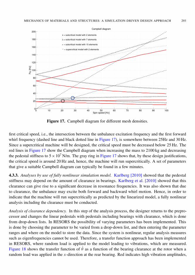
within a few seconds. Figure 17 (page 293) shows how the eigenfrequencies as a function of spin speed(Campbell diagram) depend on the mesh density of the case studied (the black dots, triangles and plusmarkers). From this figure it can be concluded that, except for the second forward whirl mode at largespin speeds, the eigenfrequencies show little mesh density dependency.

In this scenario, a machine running just above the first forward whirl frequency is to be designed and,hence, even the coarsest mesh gives enough accuracy and will therefore be used henceforth.

Selection of pedestal stiffness and rotor mass. When a suitable mesh density has been obtained, thedesigner can test different concepts by changing parameters in the preprocessor, conduct numerical sim-ulation (when needed) and postprocess and analyze the results. The blue ring in Figure 17 shows that the

MECHANICS OF MATERIALS AND STRUCTURES: A SIMULATION-DRIVEN DESIGN APPROACH 293

0 10 20 30 40 50 60 70 80 90 1000

20

40

60

80

100

120

140

160

180

200Campbell diagram

Spin speed [Hz]

Fq

. [H

z]

• = subcritical model with 2 elements

∆ = subcritical model with 7 elements

+ = subcritical model with 15 elements

− = supercritical model with 2 elements

Figure 17. Campbell diagram for different mesh densities.

first critical speed, i.e., the intersection between the unbalance excitation frequency and the first forwardwhirl frequency (dashed line and black dotted line in Figure 17), is somewhere between 25Hz and 30 Hz.Since a supercritical machine will be designed, the critical speed must be decreased below 25 Hz. Thered lines in Figure 17 show the Campbell diagram when increasing the mass to 2100 kg and decreasingthe pedestal stiffness to 5×107 N/m. The gray ring in Figure 17 shows that, by these design justifications,the critical speed is around 20 Hz and, hence, the machine will run supercritically. A set of parametersthat give a suitable Campbell diagram can typically be found in a few minutes.

4.3.3. Analyses by use of fully nonlinear simulation model. Karlberg [2010] showed that the pedestalstiffness may depend on the amount of clearance in bearings. Karlberg et al. [2010] showed that thisclearance can give rise to a significant decrease in resonance frequencies. It was also shown that dueto clearance, the unbalance may excite both forward and backward whirl motion. Hence, in order toindicate that the machine will run supercritically as predicted by the linearized model, a fully nonlinearanalysis including the clearance must be conducted.

Analysis of clearance dependency. In this step of the analysis process, the designer returns to the prepro-cessor and changes the linear pedestals with pedestals including bearings with clearance, which is donefrom drop-down lists. In RESORS the possibility of varying parameters has been implemented. Thisis done by choosing the parameter to be varied from a drop-down list, and then entering the parameterranges and where on the model to store the data. Since the system is nonlinear, regular analysis measuressuch as eigenfrequencies cannot be used. Therefore, a transfer function approach has been implementedin RESORS, where random load is applied to the model leading to vibrations, which are measured.Figure 18 shows the transfer function of θ as a function of the bearing clearance at the rotor when arandom load was applied in the x-direction at the rear bearing. Red indicates high vibration amplitudes,

294 L. KARLSSON, A. PAHKAMAA, M. KARLBERG, M. LÖFSTRAND, J. GOLDAK AND J. PAVASSON

Figure 18. Resonance frequencies as a function of bearing clearance.

while blue indicates low vibration amplitudes. The model has a spin speed of 25 Hz Figure 18 showsthat the first four eigenfrequencies at zero clearance are 16 Hz, 18 Hz, 58 Hz and 92 Hz.

Figure 18 shows that when the clearance in the bearings is increased to 0.2 mm the resonance frequen-cies decrease up to 20 Hz. The resonance frequencies within this clearance range do not coincide withthe spin speed, but a clearance below 0.1 mm is still recommended, since the first multiple of the spinspeed (50 Hz) may also excite the system and hence cause resonance. In order to verify that a suitabledesign has been developed, in the final step the designer runs an unbalance response simulation of thefully nonlinear model. The dashed line in Figure 19 is the unbalance response for the largest acceptableclearance (0.1 mm). As a reference, the unbalance response of the linearized model is also shown (solidline in Figure 19). Unlike the linear model, analysis of the nonlinear unbalance response shows thatcritical speeds can occur at more intersections than between the spin speed and the first forward whirlfrequency.

The time needed to conduct the nonlinear analysis described above is usually around one hour.

4.4. Rotor dynamical case discussion. To show how simulation-driven rotor dynamical design can beconducted a tool named RESORS has been developed and evaluated. The proposed methodology consistsof three steps: gathering of information, analysis by use of linearized models, and by use of nonlinearmodels.

In RESORS, information based on expert knowledge has been implemented, such as different pedestaltypes, choice of damping parameters, postprocessing tools as transfer functions for nonlinear systems,etc., meaning that the designer does not have to bother about rotor dynamical details. The GUI ofRESORS has further been designed to be intuitive and easy to use, featuring e.g., clear descriptionsof in-data fields and units, drop-down lists for specific choices, few steps in pre and postprocessing,etc. The post processor in RESORS is designed so that important engineering measures are directlyderived without further data processing, e.g., Campbell diagrams, mode shapes, transfer functions andload responses (maximum vibration amplitudes).

MECHANICS OF MATERIALS AND STRUCTURES: A SIMULATION-DRIVEN DESIGN APPROACH 295

0 10 20 30 40 50 60 70 80 90 1000

0.5

1

1.5

2

2.5

3x 10

−5 Unbalance Response

Ω [Hz]

Max A

mp [ra

d/s

]

Figure 19. Unbalance response of linearized model (solid line) and nonlinear model(dashed line).

For the specific case used in this paper an overcritical rotating machine including bearings with clear-ance was to be developed, meaning that the system becomes strongly nonlinear and, hence, traditionalanalysis fails. By comparing the results from the linearized model (used to derive a suitable mesh den-sity) with the results from the fully nonlinear model it was found that the resonance frequencies have astrong dependency on the clearance. Hence, a nonlinear analysis is necessary when designing rotatingmachinery supported on bearings with clearance. Although advanced equations and simulation strategiesare required for this type of analysis, with RESORS, analysis is still easy for the designer.

The total time to finish one loop of the proposed three-step methodology is typically around one anda half hours, to be compared with traditional “over the wall” strategies, which usually take days or evenweeks per iteration. Hence, by use of the proposed simulation-driven design methodology and effectiveand intuitive simulation software, a lot of time is saved (days or even weeks). This time can insteadbe used to test other possible solutions to the problem — in other words, a larger design space can beexplored, thereby improving the innovation probability.

5. Conclusions

To show how tools for modeling and simulation of mechanics of materials and structures can be designedand used to enable simulation-driven product development two case studies have been used. In both cases,fundamental equations as discussed in Sections 3.1 and 4.1, serve as basis for the software design anddevelopment in this paper.

The first case study concerned welding simulations of a Volvo Construction Equipment wheel loaderrear axle bridge (mechanics of materials), while the second case study concerned design of a supercriticalrotating machine (mechanics of structures).

In the welding case study, a simulation-driven design methodology is applied in order to find suitablewelding sequences for a Volvo Construction Equipment wheel loader rear axle bridge. It can be concluded

296 L. KARLSSON, A. PAHKAMAA, M. KARLBERG, M. LÖFSTRAND, J. GOLDAK AND J. PAVASSON

that by use of a calibrated mesh density and block dumping heat source, the efficiency of the weldingsimulations was improved with sufficient simulation accuracy.

A program (RESORS) enabling simulation-driven design has been developed and used for the rotordynamical case study. This software has been designed for improved usability compared to commercialcodes used for rotor dynamical analysis through the GUI, being developed purposely for the specificapplication. The software has been found to be intuitive, efficient and easy to use for designers andimproves postprocessing and analysis even for challenging, nonlinear problems.

The methodology used in the two widely different cases both shows that the efficiency in the analysisof challenging problems can be significantly improved through developing advanced tools suitable for useby design engineers. Important features for enabling simulation design by designers are (i) a graphicaluse interface enabling simulation-driven design; (ii) software built on ambient expert knowledge, madeusable for the designer; (iii) significantly decreased time from preprocessing to analysis compared tocommercially available codes; and (iv) postprocessing and analysis made easy for designers.

These two examples of simulation-driven design by designers indicate that a larger design space canbe explored and that more possible solutions can be evaluated. Therefore, the approach improves theprobabilities of innovation and finding optimal solutions.

Furthermore, the calibrated block dumping results presented in Section 3.3 can be used to increasethe efficiency of welding simulations when many simulations are required.

References

[Andersson 1978] B. A. B. Andersson, “Thermal stresses in a submerged-arc welded joint considering phase transformations”,J. Eng. Mater. Technol. (ASME) 100:4 (1978), 356–362.

[Åström 2004] P. Åström, Simulation of manufacturing processes in product development, Ph.D. thesis, Luleå University ofTechnology, Luleå, 2004, Available at http://epubl.ltu.se/1402-1544/2004/56/index-en.html.

[Barroso et al. 2010] A. Barroso et al., “Prediction of welding residual stresses and displacements by simplified models: exper-imental validation”, Mater. Des. 31:3 (2010), 1338–1349.

[Bylund 2004] N. Bylund, Simulation driven product development applied to car body design, Ph.D. thesis, Luleå Universityof Technology, Luleå, 2004, Available at http://epubl.luth.se/1402-1544/2004/33/index-en.html.

[Cai and Zhao 2003] Z. Cai and H. Zhao, “Efficient finite element approach for modelling of actual welded structures”, Sci.Technol. Weld. Join. 8:3 (2003), 195–204.

[Chen and Sheng 1992] Y. Chen and I. C. Sheng, “Residual stress in weldment”, J. Therm. Stresses 15:1 (1992), 53–69.

[Childs 1982] D. W. Childs, “Fractional-frequency rotor motion due to nonsymmetric clearance effects”, J. Eng. Power 104:3(1982), 533–541.

[Childs 1993] D. Childs, Turbomachinery rotordynamics: phenomena, modeling and analysis, Wiley, New York, 1993.

[Chu and Zhang 1997] F. Chu and Z. Zhang, “Periodic, quasi-periodic and chaotic vibrations of a rub-impact rotor systemsupported on oil film bearings”, Int. J. Eng. Sci. 35:10–11 (1997), 963–973.

[Courter 2009] B. Courter, “Simulation-driven product development: will form finally follow function?”, White paper, Space-Claim, Concord, MA, 2009, Available at http://files.spaceclaim.com/whitepapers/SPC.CAE.WhitePaper.web2.pdf.

[Cross 2000] N. Cross, Engineering design methods: strategies for product design, Wiley, Chichester, 2000.

[Deng et al. 2009] D. Deng, K. Ogawa, S. Kiyoshima, N. Yanagida, and K. Saito, “Prediction of residual stresses in a dissimilarmetal welded pipe with considering cladding, buttering and post weld heat treatment”, Comput. Mater. Sci. 47:2 (2009), 398–408.

[Edwards et al. 1999] S. Edwards, A. W. Lees, and M. I. Friswell, “The influence of torsion on rotor/stator contact in rotatingmachinery”, J. Sound Vib. 225:4 (1999), 767–778.

MECHANICS OF MATERIALS AND STRUCTURES: A SIMULATION-DRIVEN DESIGN APPROACH 297

[Ganesan 1996] R. Ganesan, “Dynamic response and stability of a rotor-support system with non-symmetric bearing clear-ances”, Mech. Mach. Theory 31:6 (1996), 781–798.

[Genta 1999] G. Genta, Vibration of structures and machines: practical aspects, Springer, New York, 1999.

[Gero 1981] J. S. Gero, “Design optimization”, Comput.-Aided Des. 13:5 (1981), 252.

[Goldak 2009] J. A. Goldak, “Distortion and residual stress in welds: the next generation”, pp. 45–52 in Trends in weldingresearch: proceedings of the 8th International Conference (Pine Mountain, GA, 2008), edited by S. A. David et al., ASMInternational, Materials Park, OH, 2009.

[Goldak and Akhlaghi 2005] J. A. Goldak and M. Akhlaghi, Computational welding mechanics, Springer, New York, 2005.

[Goldak et al. 1986] J. A. Goldak, B. Patel, M. Bibby, and J. Moore, “Computational weld mechanics”, AGARD Conf. Proc.398 (1986), 1–32.

[Goldak et al. 2007] J. A. Goldak et al., “Designer driven analysis of welded structures”, pp. 1025–1038 in Mathematicalmodelling of weld phenomena 8 (Graz, 2006), edited by H.-H. Cerjak et al., Technische Universität Graz, Graz, 2007.

[Goldak Technologies 2010] Goldak Technologies, “VrWeld”, 2010, Available at http://www.goldaktec.com/vrweld.html.

[Goldman and Muszynska 1995] P. Goldman and A. Muszynska, “Rotor-to-stator, rub-related, thermal/mechanical effects inrotating machinery”, Chaos Solitons Fractals 5:9 (1995), 1579–1601.

[Hansen 1974] H. R. Hansen, “Application of optimization methods within structural design: practical design example”, Com-put. Struct. 4:1 (1974), 213–220.

[Harris 1991] T. A. Harris, Rolling bearing analysis, Wiley, New York, 1991.

[Jeffcott 1919] H. H. Jeffcott, “XXVII. The lateral vibration of loaded shafts in the neighbourhood of a whirling speed.–Theeffect of want of balance”, Philos. Mag. (6) 37:219 (1919), 304–314.

[Karlberg 2010] M. Karlberg, “Approximated stiffness coefficients in rotor systems supported by bearings with clearance”, Int.J. Rotat. Mach. 2010 (2010). Article ID 540101.

[Karlberg and Aidanpää 2003] M. Karlberg and J.-O. Aidanpää, “Numerical investigation of an unbalanced rotor system withbearing clearance”, Chaos Solitons Fractals 18:4 (2003), 653–664.

[Karlberg and Aidanpää 2004] M. Karlberg and J.-O. Aidanpää, “Investigation of an unbalanced rotor system with bearingclearance and stabilising rods”, Chaos Solitons Fractals 20:2 (2004), 363–374.

[Karlberg and Aidanpää 2007] M. Karlberg and J.-O. Aidanpää, “Rotordynamical modelling of a fibre refiner during produc-tion”, J. Sound Vib. 303:3–5 (2007), 440–454.

[Karlberg et al. 2010] M. Karlberg, M. Karlsson, L. Karlsson, and M. Näsström, “Dynamics of rotor systems with clearanceand weak pedestals in full contact”, in 13th International Symposium on Transport Phenomena and Dynamics of RotatingMachinery: ISROMAC 13 (Honolulu, HI, 2010), International Symposium on Transport Phenomena and Dynamics of RotatingMachinery 13, Curran Associates, Red Hook, NY, 2010.

[Karlsson 1986] L. Karlsson, “Thermal stresses in welding”, pp. 299–389 in Thermal stresses I, edited by R. B. Hetnarski,Elsevier, Amsterdam, 1986.

[Karlsson et al. 1989] L. Karlsson, M. Jonsson, L.-E. Lindgren, M. Näsström, and L. Troive, “Residual stresses and deforma-tions in a welded thin-walled pipe”, pp. 7–11 in Weld residual stresses and plastic deformation (Honolulu, HI, 1989), editedby E. Rybicki et al., Pressure Vessels and Piping 173, ASME, New York, 1989.

[LaCourse 1995] D. E. LaCourse, Handbook of solid modeling, McGraw-Hill, New York, 1995.

[Lee et al. 2008] C.-H. Lee, K.-H. Chang, and C.-Y. Lee, “Comparative study of welding residual stresses in carbon andstainless steel butt welds”, Proc. Inst. Mech. Eng. B, J. Eng. Manuf. 222:12 (2008), 1685–1694.

[Lindgren 2001a] L.-E. Lindgren, “Finite element modeling and simulation of welding, 2: Improved material modeling”, J.Therm. Stresses 24:3 (2001), 195–231.

[Lindgren 2001b] L.-E. Lindgren, “Finite element modeling and simulation of welding, 1: Increased complexity”, J. Therm.Stresses 24:2 (2001), 141–192.

[Lindgren 2001c] L.-E. Lindgren, “Finite element modeling and simulation of welding, 3: Efficiency and integration”, J. Therm.Stresses 24:4 (2001), 305–334.

298 L. KARLSSON, A. PAHKAMAA, M. KARLBERG, M. LÖFSTRAND, J. GOLDAK AND J. PAVASSON

[Lindgren 2007] L.-E. Lindgren, Computational welding mechanics: thermomechanical and microstructural simulations, CRCPress, Boca Raton, FL, 2007.

[Mochizuki et al. 2000] M. Mochizuki, M. Hayashi, and T. Hattori, “Numerical analysis of welding residual stress and itsverification using neutron diffraction measurement”, J. Eng. Mater. Technol. (ASME) 122:1 (2000), 98–103.

[Muszynska and Goldman 1995] A. Muszynska and P. Goldman, “Chaotic responses of unbalanced rotor/bearing/stator sys-tems with looseness or rubs”, Chaos Solitons Fractals 5:9 (1995), 1683–1704.

[Ogawa et al. 2009] K. Ogawa, D. Deng, S. Kiyoshima, N. Yanagida, and K. Saito, “Investigations on welding residual stressesin penetration nozzles by means of 3D thermal elastic plastic FEM and experiment”, Comput. Mater. Sci. 45:4 (2009), 1031–1042.

[Pahkamaa et al. 2010] A. Pahkamaa, L. Karlsson, and J. Pavasson, “A method to improve efficiency in welding simulationsfor simulation driven design”, pp. 81–90 in Proceedings of the ASME International Design Engineering Technical Confer-ences and Computers and Information in Engineering Conference (IDETC/CIE2010), 3: 30th Computers and Information inEngineering Conference (Montreal, 2010), ASME, New York, 2010.

[Ramm 1981] E. Ramm, Nonlinear finite element analysis in structural mechanics: strategies for tracing the nonlinear re-sponse of near limit points, Springer, Berlin, 1981.

[Rankine 1869] W. A. Rankine, “On the centrifugal force of rotating shafts”, Eng. 27 (1869), 249.

[Saad 1996] Y. Saad, Iterative methods for sparse linear systems, PWS, Boston, 1996. 2nd ed. published by SIAM, Philadel-phia, 2003.

[Sellgren 1995] U. Sellgren, Simulation driven design: a functional view of the design process, Licentiate thesis, Royal Instituteof Technology, Stockholm, 1995, Available at http://www.md.kth.se/~ulfs/Research/LIC/LIC_main.pdf.

[Smith and Reinertsen 1998] P. G. Smith and D. G. Reinertsen, Developing products in half the time: new rules, new tools,Wiley, New York, 1998.

[Smith and Smith 2009a] M. C. Smith and A. C. Smith, “NeT bead-on-plate round robin: comparison of residual stress predic-tions and measurements”, Int. J. Press. Vessels Pip. 86:1 (2009), 79–95.

[Smith and Smith 2009b] M. C. Smith and A. C. Smith, “NeT bead-on-plate round robin: comparison of transient thermalpredictions and measurements”, Int. J. Press. Vessels Pip. 86:1 (2009), 96–109.

[Troive et al. 1998] L. Troive, M. Näsström, and M. Jonsson, “Experimental and numerical study of multi-pass welding processof pipe-flange joints”, J. Press. Vessel Technol. (ASME) 120:3 (1998), 244–251.

[Truman and Smith 2009] C. E. Truman and M. C. Smith, “The NeT residual stress measurement and modelling round robinon a single weld bead-on-plate specimen”, Int. J. Press. Vessels Pip. 86:1 (2009), 1–2.

[Ueda and Yuan 1993] Y. Ueda and M. G. Yuan, “Prediction of residual stresses in butt welded plates using inherent strains”,J. Eng. Mater. Technol. (ASME) 115:4 (1993), 417–423.

[Ueda et al. 1986] Y. Ueda, K. Fukuda, and Y. C. Kim, “New measuring method of axisymmetric three-dimensional residualstresses using inherent strains as parameters”, J. Eng. Mater. Technol. (ASME) 108:4 (1986), 328–334.

[Ueda et al. 1988] Y. Ueda, Y. C. Kim, and M. G. Yuan, “A predicting method of welding residual stress using source ofresidual stress”, Q. J. Jpn. Weld. Soc. 6:1 (1988), 59–64.

[Ulrich and Eppinger 1995] K. T. Ulrich and S. D. Eppinger, Product design and development, McGraw-Hill, New York, 1995.

[Voutchkov et al. 2005] I. Voutchkov, A. J. Keane, A. Bhaskar, and T. M. Olsen, “Weld sequence optimization: the use ofsurrogate models for solving sequential combinatorial problems”, Comput. Methods Appl. Mech. Eng. 194:30–33 (2005),3535–3551.

[Wall 2007] J. Wall, Simulation-driven design of complex mechanical and mechatronic systems, Ph.D. thesis, Blekinge Instituteof Technology, Karlskrona, 2007, Available at http://tinyurl.com/Wall-2007-diss.

[Wheelwright and Clark 1992] S. C. Wheelwright and K. B. Clark, Revolutionizing product development: quantum leaps inspeed, efficiency and quality, Free Press, New York, 1992.

[Wriggers and Simo 1990] P. Wriggers and J. C. Simo, “A general procedure for the direct computation of turning and bifurca-tion points”, Int. J. Numer. Methods Eng. 30:1 (1990), 155–176.

MECHANICS OF MATERIALS AND STRUCTURES: A SIMULATION-DRIVEN DESIGN APPROACH 299

Appendix: Design space exploration: simulated welding sequences

Sequence

number

Welding sequence WeldPath nbSubPasses StartWF

1st | 2nd

EndWF

1st | 2nd

StartTime (s)

1st | 2nd

Dump and

Mesh

Calibration

a (1)

b (2)

c (3,4)

d (5,6)

1

1

2

2

0.0

1.0

0.0 | 1.0

0.0 | 1.0

1.0

0.0

0.5 | 0.5

0.5 | 0.5

0

158

317 | 396

475 | 554

1

a (1)

b (2)

c (3)

d (4)

1

1

1

1

0.0

0.0

0.0

0.0

1.0

1.0

1.0

1.0

0

158

317

475

2

a (1)

b (3)

c (2)

d (4)

1

1

1

1

0.0

0.0

0.0

0.0

1.0

1.0

1.0

1.0

0

317

158

475

3

a (1)

b (2)

c (3)

d (4)

1

1

1

1

0.0

1.0

0.0

1.0

1.0

0.0

1.0

0.0

0

158

317

475

4

a (1)

b (3)

c (2)

d (4)

1

1

1

1

0.0

1.0

0.0

1.0

1.0

0.0

1.0

0.0

0

317

158

475

5

a (1,2)

b (3,4)

c (5,6)

d (7,8)

2

2

2

2

0.0 | 1.0

0.0 | 1.0

0.0 | 1.0

0.0 | 1.0

0.5 | 0.5

0.5 | 0.5

0.5 | 0.5

0.5 | 0.5

0 | 79

158 | 237

317 | 396

475 | 554

6

a (1,2)

b (3,4)

c (5,6)

d (7,8)

2

2

2

2

0.5 | 0.5

0.5 | 0.5

0.5 | 0.5

0.5 | 0.5

0.0 | 1.0

0.0 | 1.0

0.0 | 1.0

0.0 | 1.0

0 | 79

158 | 237

317 | 396

475 | 554

7

a (1,2)

b (3,4)

c (5,6)

d (7,8)

2

2

2

2

0.5 | 0.5

0.5 | 0.5

0.0 | 1.0

0.0 | 1.0

0.0 | 1.0

0.0 | 1.0

0.5 | 0.5

0.5 | 0.5

0 | 79

158 | 237

317 | 396

475 | 554

8

a (1,2)

b (3,4)

c (5,6)

d (7,8)

2

2

2

2

0.5 | 0.5

0.0 | 1.0

0.5 | 0.5

0.0 | 1.0

0.0 | 1.0

0.5 | 0.5

0.0 | 1.0

0.5 | 0.5

0 | 79

158 | 237

317 | 396

475 | 554

9

a (1,3)

b (2,4)

c (5,7)

d (6,8)

2

2

2

2

0.0 | 1.0

1.0 | 0.0

0.0 | 1.0

1.0 | 0.0

0.5 | 0.5

0.5 | 0.5

0.5 | 0.5

0.5 | 0.5

0 | 158

79 | 237

317 | 475

396 | 554

300 L. KARLSSON, A. PAHKAMAA, M. KARLBERG, M. LÖFSTRAND, J. GOLDAK AND J. PAVASSON

10

a (1,3)

b (2,4)

c (5,7)

d (6,8)

2

2

2

2

0.5 | 0.5

0.5 | 0.5

0.5 | 0.5

0.5 | 0.5

0.0 | 1.0

1.0 | 0.0

0.0 | 1.0

1.0 | 0.0

0 | 158

79 | 237

317 | 475

396 | 554

11

a (1,2)

b (3,4)

c (5,6)

d (7,8)

2

2

2

2

0.5 | 0.0

0.5 | 0.0

0.5 | 0.0

0.5 | 0.0

1.0 | 0.5

1.0 | 0.5

1.0 | 0.5

1.0 | 0.5

0 | 79

158 | 237

317 | 396

475 | 554

12

a (1,2)

b (3,4)

c (5,6)

d (7,8)

2

2

2

2

0.5 | 1.0

0.5 | 1.0

0.5 | 0.0

0.5 | 0.0

0.0 | 0.5

0.0 | 0.5

1.0 | 0.5

1.0 | 0.5

0 | 79

158 | 237

317 | 396

475 | 554

13

a (1,2)

b (3,4)

c (5,6)

d (7,8)

2

2

2

2

0.5 | 1.0

0.5 | 0.0

0.5 | 1.0

0.5 | 0.0

0.0 | 0.5

1.0 | 0.5

0.0 | 0.5

1.0 | 0.5

0 | 79

158 | 237

317 | 396

475 | 554

14

a (1,3)

b (2,4)

c (5,7)

d (6,8)

2

2

2

2

0.0 | 1.0

0.0 | 1.0

0.0 | 1.0

0.0 | 1.0

0.5 | 0.5

0.5 | 0.5

0.5 | 0.5

0.5 | 0.5

0 | 158

79 | 237

317 | 475

396 | 554

15

a (1,3)

b (2,4)

c (5,7)

d (6,8)

2

2

2

2

0.5 | 0.5

0.5 | 0.5

0.5 | 0.5

0.5 | 0.5

0.0 | 1.0

0.0 | 1.0

0.0 | 1.0

0.0 | 1.0

0 | 158

79 | 237

317 | 475

396 | 554

16

a (1,4)

b (2,3)

c (5,8)

d (6,7)

2

2

2

2

0.0 | 1.0

0.0 | 1.0

0.0 | 1.0

0.0 | 1.0

0.5 | 0.5

0.5 | 0.5

0.5 | 0.5

0.5 | 0.5

0 | 237

79 | 158

317 | 554

396 | 475

17

a (1,4)

b (2,3)

c (5,8)

d (6,7)

2

2

2

2

0.5 | 0.5

0.5 | 0.5

0.5 | 0.5

0.5 | 0.5

0.0 | 1.0

0.0 | 1.0

0.0 | 1.0

0.0 | 1.0

0 | 237

79 | 158

317 | 554

396 | 475

18

a (1,5)

b (2,6)

c (3,7)

d (4,8)

2

2

2

2

0.0 | 1.0

0.0 | 1.0

0.0 | 1.0

0.0 | 1.0

0.5 | 0.5

0.5 | 0.5

0.5 | 0.5

0.5 | 0.5

0 | 317

79 | 396

158 | 475

237 | 554

19

a (1,5)

b (2,6)

c (3,7)

d (4,8)

2

2

2

2

0.5 | 0.5

0.5 | 0.5

0.5 | 0.5

0.5 | 0.5

0.0 | 1.0

0.0 | 1.0

0.0 | 1.0

0.0 | 1.0

0 | 317

79 | 396

158 | 475

237 | 554

20

a (1)

b (2)

c (4,6)

d (3,5)

1

1

2

2

1.0

0.0

1.0 | 0.0

1.0 | 0.0

0.0

1.0

0.5 | 0.5

0.5 | 0.5

0

158

396 | 554

317 | 475

MECHANICS OF MATERIALS AND STRUCTURES: A SIMULATION-DRIVEN DESIGN APPROACH 301

Received 30 Mar 2010. Revised 23 Jun 2010. Accepted 6 Jul 2010.

LENNART KARLSSON: Lennart.Karlsson@ltu.seThe Faste Laboratory, Division of Computer Aided Design, Luleå University of Technology, SE-97187 Luleå, Swedenhttp://www.ltu.se/tfm/cad/home/d743/d18287/leka?l=en

ANDREAS PAHKAMAA: Andreas.Pahkamaa@ltu.seDivision of Computer Aided Design, LuleåUniversity of Technology, SE-97187 Luleå, Swedenhttp://www.ltu.se/tfm/cad/home/d743/d18287/1.52354?l=en

MAGNUS KARLBERG: Magnus.Karlberg@ltu.seThe Faste Laboratory, Division of Computer Aided Design, Luleå University of Technology, SE-97187 Luleå, Swedenhttp://www.ltu.se/tfm/cad/home/d743/d18287/magkar?l=en

MAGNUS LÖFSTRAND: Magnus.Lofstrand@ltu.seThe Faste Laboratory, Division of Computer Aided Design, Luleå University of Technology, SE-97187 Luleå, Swedenhttp://www.ltu.se/tfm/cad/home/d743/d18287/maglof?l=en

JOHN GOLDAK: jgoldak@mrco2.carleton.caDepartment of Mechanical and Aerospace Engineering, Carleton University, Ottawa, ON K1S 5B6, Canada

JONAS PAVASSON: Jonas.Pavasson@ltu.seThe Faste Laboratory, Division of Computer Aided Design, Luleå University of Technology, SE-97187 Luleå, Swedenhttp://www.ltu.se/tfm/cad/home/d743/d18287/jonpav?l=en

mathematical sciences publishers msp