Journal of

Mechanics ofMaterials and Structures

REMARKS ON THE ACCURACY OF ALGORITHMS FOR MOTIONBY MEAN CURVATURE IN BOUNDED DOMAINS

Simon Cox and Gennady Mishuris

Volume 4, Nº 9 November 2009

mathematical sciences publishers

JOURNAL OF MECHANICS OF MATERIALS AND STRUCTURESVol. 4, No. 9, 2009

REMARKS ON THE ACCURACY OF ALGORITHMS FOR MOTIONBY MEAN CURVATURE IN BOUNDED DOMAINS

SIMON COX AND GENNADY MISHURIS

Simulations of motion by mean curvature in bounded domains, with applications to bubble motion andgrain growth, rely upon boundary conditions that are not necessarily compatible with the equation ofmotion. Three closed form solutions for the problem exist, governing translation, rotation, and expansionof a single interface, providing the only benchmarks for algorithm verification. We derive new identitiesfor the translation solution. Then we estimate the accuracy of a straightforward algorithm to recover theanalytical solution for different values of the velocity V given along the boundary. As expected, for largeV the error can reach unacceptable levels especially near the boundary. We discuss factors influencingthe accuracy and propose a simple modification of the algorithm which improves the computationalaccuracy.

1. Introduction

Motion by mean curvature and the dynamics of two-dimensional foams are closely related subjectsin the study of materials [Smith 1952]. In the ideal model of the evolution of crystalline grains in apolycrystalline metal, known as normal grain growth, the size of each grain evolves due to the normalmotion of each of its boundaries [Weaire and McMurry 1996]. Each boundary has a certain mobility λ,and moves in such a way as to reduce the total perimeter of the pattern. The ideal soap froth is a modelof a two-dimensional foam [Weaire and Hutzler 1999], such as the one studied by Bragg and Nye [1947]and which has recently enjoyed a renaissance, in which interface curvature and pressure differences arebalanced, again due to minimization of the total perimeter. Both ideal models arise naturally as limits ofthe following viscous froth model (VFM) [Kern et al. 2004], derived as a force balance per unit lengthof the interface:

1p = γ κ + λvn. (1-1)

Here 1p is the pressure difference across the interface and γ its surface tension (assumed constant); κis the local curvature and vn the velocity normal to the interface.

The aim of this paper is to investigate the accuracy of algorithms for (1-1), and for this reason werestrict ourselves to the simplest case, when 1p = 0. In the case of grain growth, there are no area(volume in 3D) constraints, and pressure differences between cells are negligible. This limit is alsoappropriate to ordered (hexagonal) foams and single soap films.

We ask how a solution to the equations of motion by mean curvature can be commensurate with theboundary of the domain. That is, even though we can find an interface shape at a particular instantin time, by solving the governing equation, it is not always possible to match this with the imposed

Keywords: motion by mean curvature, grain growth, foam rheology, algorithms, measures of accuracy.Cox was financially supported by EPSRC (EP/D048397/1, EP/D071127/1).

1555

1556 SIMON COX AND GENNADY MISHURIS

boundary condition on velocity. We then ask how well solutions that satisfy both the governing equationand boundary condition can be calculated numerically.

The most stringent test of a numerical algorithm here is an initial interface shape that is far fromsatisfying the boundary conditions. It is this that we use for our preliminary numerical tests. We developa general class of less severe solutions, that can be used to test numerical algorithms, based upon thissimple interface shape (rather than the more complicated shapes found in a real foam or metal). Wepropose three identities which provide measures of accuracy and, further, can be implemented within anexisting algorithm to improve its performance.

2. Curvature-driven motion of a bounded interface

2A. Problem formulation. In vector form, the motion of an interface in the model of ideal grain growthcan be described by

v = κn, (2-1)

where n and s are the normal and tangential unit vectors to the interface (see Figure 1):

n= [n1, n2], s = [n2,−n1]. (2-2)

If the representation of the interface is taken in the form

x = x(y, t), y ∈ [y(t), y(t)], (2-3)

then the vector components n1, n2 are calculated as follows:

n1 =−dyds=− sin θ =−

1√1+ (xy)2

, n2 =dxds= cos θ =

xy√1+ (xy)2

, (2-4)

where xy = dx/dy, ds =√(dx)2+ (dy)2, and θ is the tangential angle to the interface (see Figure 1).

Finally, the vector v = [v1, v2] is the instantaneous velocity of the point (x, y) lying on the interface attime t and κ is the curvature of the interface at that point:

κ =dθds=

−xyy√(1+ (xy)2)3

. (2-5)

θ

sn

y

y

x

y

Figure 1. The bounded interface considered here.

ACCURACY OF ALGORITHMS FOR MOTION BY MEAN CURVATURE IN BOUNDED DOMAINS 1557

Equation (2-1) can also be written in component form:

vn = v · n= v1n1+ v2n2 = κ, (2-6)

vs = v · s = v1n2− v2n1 = 0. (2-7)

In this paper we will consider only Mullins’ translational solution [Mullins 1956] (see below), also knownas the grim reaper because of the way in which it scythes through space without change of shape, whichis symmetrical with respect to the x-axis. Invariant solutions for rotation have been considered elsewhere[Mullins 1956; Wood 1996]. Taking into account the direction of the interface motion, we can assumethat

n1 < 0, n2 > 0, xy > 0, 0< θ < π/2, xyy > 0, κ < 0, (2-8)

vn < 0 (v2 < 0, v1 > 0). (2-9)

Equation (2-6) is widely discussed in the literature [Mullins 1956; Peleg et al. 2001], while (2-7) issomehow usually forgotten in this context. If one is only interested in reconstructing the interface positionat any time step an approach based only on (2-6) is sufficient. However, if it is required that the positionof each material point along the interface is controlled, as in the case of numerical computation, thenboth equations are equally important. Note that there has previously been an attempt to control both thevelocity components in a specific way [Green et al. 2006]. Equation (2-7) allows us to find a relationbetween the two unknown components of the velocity vector v and the normal vector n in the form

n2 =v2v1

n1. (2-10)

This allows us to eliminate components of the normal vector n from (2-6) to give

−

(v1+

v22

v1

)=

dθdy. (2-11)

2B. Mullins’ solution for translation revisited. Let us assume that the interface conserves its shape butmoves in the x-direction with a constant speed V . We consider two points A and C having the samey-coordinate y = y0 at two consecutive time steps t0 and t0 + dt (see Figure 2). It is clear that thesetwo points correspond to two different material points. Namely, there exists a point B on the interface at

A

B

C

y

x

y0

y + dy0

x0

x + dx0

t + dt0

t 0

θ

Figure 2. Interface under translational motion at two consecutive instants in time.

1558 SIMON COX AND GENNADY MISHURIS

time t0 which moves according to the curvature law (2-1) to the point C for an infinitesimally small timestep dt . If the coordinates of the point A are (x0, y0) then the coordinates of B and C can be written(x0+ dx, y0+ dy) and (x0+ V dt, y0).

Note thatBC = v(x0+ dx, y0+ dy)dt = v(x0, y0)dt + O(dt ds).

On the other hand, |BC | = V sin θ dt , and tan θ = v1/|v2|. As a result one can conclude:

V =1

v1(y)

(v2

1(y)+ v22(y)

), (2-12)

in some interval y ∈ [0, h]. This relation follows immediately from (2-11) in the case of translation ofthe interface in the x-direction.

Now, to reconstruct the solution obtained by Mullins [1956] it is sufficient to substitute (2-12) into(2-11) to give

π2− V y = θ. (2-13)

Here we have taken into account the second of the two symmetry conditions at the point y = 0:

v2(0)= 0, θ(0)= π2. (2-14)

Equation (2-13) can be written in the form

cot V y = yx , (2-15)

which after direct integration leads to Mullins’ solution:

x(y)= x(0)+ V t − 1V

log cos(V y), y ∈ [0, h], (2-16)

where x(0) is the arbitrary initial position of the centre of the interface. This solution exists only underthe condition h < hmax, where

hmax =π

2V. (2-17)

Note also that the angle θ defined by such a solution monotonically decreases in the interval y ∈ (0, h)(h < hmax), taking values

θ(y) ∈(θmin,

π2

), θmin = θmin(h)=

π2− V h. (2-18)

It is now possible to write analytical representations of all problem variables in the interval y ∈ (0, h):

v1 = V cos2 V y, v2 =−12 V sin 2V y, n1 = sin V y, n2 = cos V y, κ = V cos V y. (2-19)

Note that the first symmetry condition (2-14) has not been used but the reconstructed Mullins solution(2-16) satisfies it automatically, by (2-4) and (2-10). The solution exhibits the following asymptoticsnear the symmetry axis:

x(y)= x(0)+ V t + 12 V y2

+ O(y4), y→ 0; (2-20)

ACCURACY OF ALGORITHMS FOR MOTION BY MEAN CURVATURE IN BOUNDED DOMAINS 1559

thus near y = 0 the interface is close to a parabola. Close to the other end of the reaper (in the case ofthe maximal thickness h = hmax), the following asymptotic estimate can be obtained:

x(y)=− 1V

log(hmax− y)+O(1), y→ hmax, or y−hmax∼−de−V x , x→+∞, (2-21)

where d = (1/V ) exp{V (x(0)+ V t)} is a positive constant.Note that relation (2-12) also represents the boundary condition for any moving interface whose upper

point lies on the line y= y= h and which moves in the x-direction with velocity V . Moreover, the velocitycan be in that case a function of time V = V (t):

V (t)v1(h, t)= v21(h, t)+ v2

2(h, t). (2-22)

Substituting (2-1) into (2-22) such a boundary condition can be equivalently rewritten in other forms:

κ(h, t)= V (t)n1(h, t), or xyy(h, t)= V (t)(1+ (xy(h, t))2

). (2-23)

Note that we have not used (2-16) to define (2-23).

2C. Arbitrary instantaneous solution of equations (2-6) and (2-7) in a bounded domain. Let us con-sider any instantaneous solution of the equations (2-6) and (2-7) with the prescribed boundary condition(2-22), by which we mean an instantaneous state of the film which may or may not be commensuratewith the boundary conditions and could or could not be a steady state. Effectively this means that, fora particular time t , the end points of the interface y = y(t) and y = h are defined and the velocitycomponents v1(y, t) and v2(y, t) are known functions of the variable y, while the problem is now todetermine, using this information, the position of the interface in space variables (y, x).

We introduce a function which in what follows is considered known:

F(y)= v1(y)+v2

2(y)v1(y)

> 0, y ∈ (y, h). (2-24)

Note that the condition (2-12) may be not valid at all inside the interval y ∈ (y, h) as it was for Mullins’solution; as a result, F(y) is not a constant, in general. Equation (2-11) can be integrated to give

−

∫ y

yF(ξ)dξ = θ(y)− θ. (2-25)

Here, recall that F depends upon time t , so that y = y(t) and the constant of integration is θ = θ(t).Equation (2-25) should be considered together with (2-10) which, in this case, takes the form

dxdy=−

v2v1= cot θ, (2-26)

or

x(y)= x −∫ y

y

v2(ξ)

v1(ξ)dξ. (2-27)

Equations (2-25) and (2-26) together indicate that the functions v1 and v2 cannot be chosen arbitrarily tosatisfy the vectorial (2-1) as one might expect. Instead, the following identity has to be satisfied:

arctan v1v2=

∫ y

yF(ξ)dξ − θ, (2-28)

1560 SIMON COX AND GENNADY MISHURIS

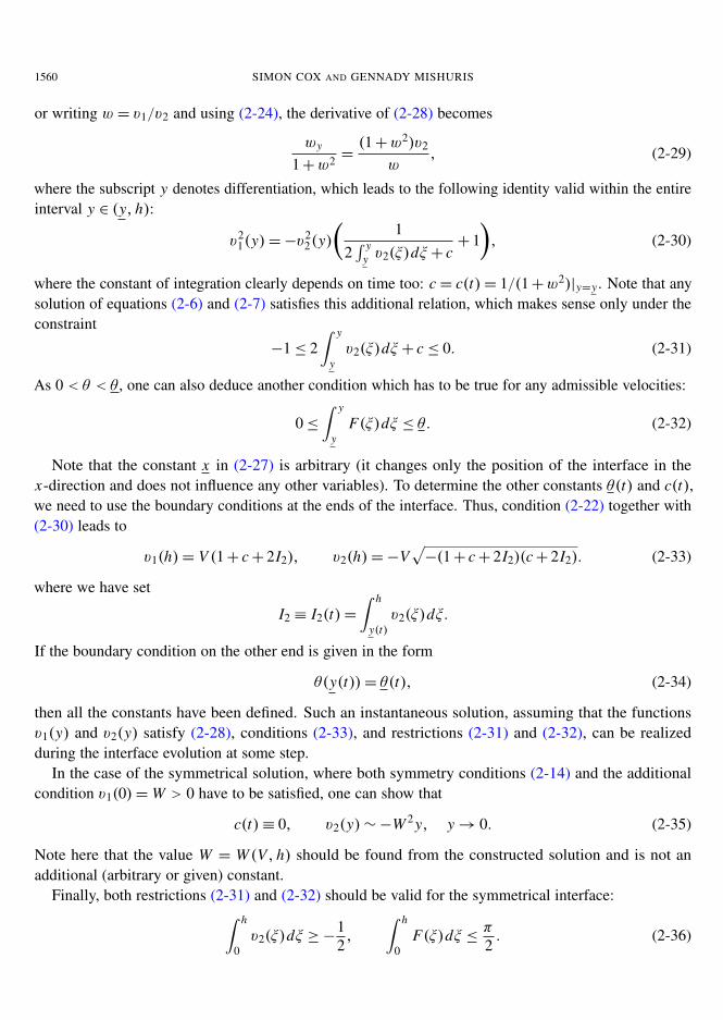
or writing w = v1/v2 and using (2-24), the derivative of (2-28) becomes

wy

1+w2 =(1+w2)v2

w, (2-29)

where the subscript y denotes differentiation, which leads to the following identity valid within the entireinterval y ∈ (y, h):

v21(y)=−v

22(y)

(1

2∫ y

y v2(ξ)dξ + c+ 1

), (2-30)

where the constant of integration clearly depends on time too: c = c(t)= 1/(1+w2)|y=y . Note that anysolution of equations (2-6) and (2-7) satisfies this additional relation, which makes sense only under theconstraint

−1≤ 2∫ y

yv2(ξ)dξ + c ≤ 0. (2-31)

As 0< θ < θ , one can also deduce another condition which has to be true for any admissible velocities:

0≤∫ y

yF(ξ)dξ ≤ θ. (2-32)

Note that the constant x in (2-27) is arbitrary (it changes only the position of the interface in thex-direction and does not influence any other variables). To determine the other constants θ(t) and c(t),we need to use the boundary conditions at the ends of the interface. Thus, condition (2-22) together with(2-30) leads to

v1(h)= V (1+ c+ 2I2), v2(h)=−V√−(1+ c+ 2I2)(c+ 2I2). (2-33)

where we have set

I2 ≡ I2(t)=∫ h

y(t)v2(ξ)dξ.

If the boundary condition on the other end is given in the form

θ(y(t))= θ(t), (2-34)

then all the constants have been defined. Such an instantaneous solution, assuming that the functionsv1(y) and v2(y) satisfy (2-28), conditions (2-33), and restrictions (2-31) and (2-32), can be realizedduring the interface evolution at some step.

In the case of the symmetrical solution, where both symmetry conditions (2-14) and the additionalcondition v1(0)=W > 0 have to be satisfied, one can show that

c(t)≡ 0, v2(y)∼−W 2 y, y→ 0. (2-35)

Note here that the value W = W (V, h) should be found from the constructed solution and is not anadditional (arbitrary or given) constant.

Finally, both restrictions (2-31) and (2-32) should be valid for the symmetrical interface:∫ h

0v2(ξ)dξ ≥−

12,

∫ h

0F(ξ)dξ ≤ π

2. (2-36)

ACCURACY OF ALGORITHMS FOR MOTION BY MEAN CURVATURE IN BOUNDED DOMAINS 1561

Note that the tangential angle θ for this solution is a monotonically decreasing function in the intervaly ∈ (0, h) so that

θ(y) ∈(θmin,

π2

), θmin =

π2−

∫ h

0F(ξ)dξ. (2-37)

It is straightforward to see that Mullins’ solution (2-19) satisfies all these relationships with c(t) = 0,θ(t)=π/2, and W = V , as expected. In the next section, we construct analytical examples of symmetricalinstantaneous solutions which are different from Mullins’.

3. A family of symmetrical instantaneous solutions

In this section we present analytical representations of some instantaneous symmetrical solutions forthe interface satisfying the same boundary (2-22) and symmetry (2-14) conditions as Mullins’ solution.Those solutions are not, generally speaking, steady-state ones. This means that they can be reached atsome time step t , given the interface boundary velocity V (t) and the position of the ends h(t), but allthese parameters may later change with time. What is extremely interesting about these solutions isthat some of them are well-defined for any velocity V > 0 and an arbitrary position of the boundaryy = h. This shows a rich behaviour of possible instantaneous solutions. It is also clear that there is aninfinite number of admissible instantaneous solutions. Some of them can be realized during some specificnon-steady-state interface motion. For example, any instantaneous solution obtained during a numericalcomputation, for any particular time step, boundary velocity, and topology, has to satisfy all the relations(2-24)–(2-34). This will allow us to use the relations as indicators of the accuracy of computations.Moreover, they could provide a means to improve the accuracy of the algorithms.

(One could also consider the family of arbitrary, not necessarily symmetric, instantaneous solutions,which is even larger than the symmetric case. In fact, the family of symmetrical solutions has onedegree of freedom — since c(t) vanishes in this case — and correspondingly one less boundary condition;compare (2-34) and (2-14). In the context of further applications of this result to a given algorithm,where the angle-type boundary condition has to be preserved at the interface intersection point, it isworth mentioning that the boundary condition (2-34) is therefore more important for application than thesymmetry condition. On the other hand, symmetrical instantaneous solutions can also be considered asubset of the asymmetric solutions if one considers the interval (h0, h) instead of (0, h) (0 < h0 < h).This idea has been exploited previously in [Green et al. 2009].)

3A. First example. We consider the following simple combination of compatible velocities

v2(y)=−W 2 y, v1(y)=W√

1−W 2 y2, W =V

√1+ V 2h2

, (3-1)

which satisfy (2-30) with c = 0 and y = 0 and, as a result, can be used to construct a symmetricalinstantaneous solution. Here W is the same constant as in (2-35). Natural restrictions (2-36) for theexistence of such a solution give the same estimate:

W <1h, or

V√

1+ V 2h2<

1h, (3-2)

1562 SIMON COX AND GENNADY MISHURIS

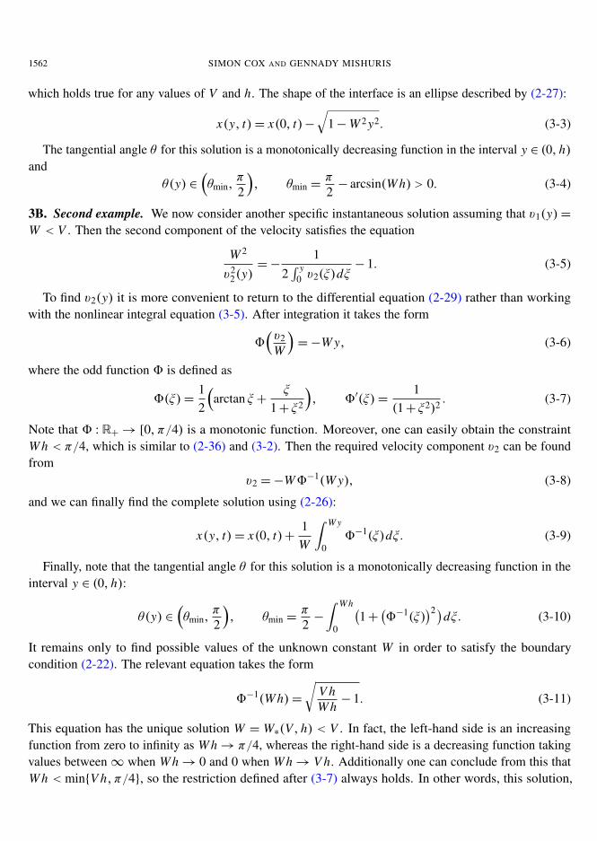
which holds true for any values of V and h. The shape of the interface is an ellipse described by (2-27):

x(y, t)= x(0, t)−√

1−W 2 y2. (3-3)

The tangential angle θ for this solution is a monotonically decreasing function in the interval y ∈ (0, h)and

θ(y) ∈(θmin,

π2

), θmin =

π2− arcsin(W h) > 0. (3-4)

3B. Second example. We now consider another specific instantaneous solution assuming that v1(y)=W < V . Then the second component of the velocity satisfies the equation

W 2

v22(y)=−

12∫ y

0 v2(ξ)dξ− 1. (3-5)

To find v2(y) it is more convenient to return to the differential equation (2-29) rather than workingwith the nonlinear integral equation (3-5). After integration it takes the form

8(v2W

)=−W y, (3-6)

where the odd function 8 is defined as

8(ξ)=12

(arctan ξ +

ξ

1+ ξ 2

), 8′(ξ)=

1(1+ ξ 2)2

. (3-7)

Note that 8 : R+→ [0, π/4) is a monotonic function. Moreover, one can easily obtain the constraintW h < π/4, which is similar to (2-36) and (3-2). Then the required velocity component v2 can be foundfrom

v2 =−W8−1(W y), (3-8)

and we can finally find the complete solution using (2-26):

x(y, t)= x(0, t)+1W

∫ W y

08−1(ξ)dξ. (3-9)

Finally, note that the tangential angle θ for this solution is a monotonically decreasing function in theinterval y ∈ (0, h):

θ(y) ∈(θmin,

π2

), θmin =

π2−

∫ W h

0

(1+

(8−1(ξ)

)2 )dξ. (3-10)

It remains only to find possible values of the unknown constant W in order to satisfy the boundarycondition (2-22). The relevant equation takes the form

8−1(W h)=

√V hW h− 1. (3-11)

This equation has the unique solution W = W∗(V, h) < V . In fact, the left-hand side is an increasingfunction from zero to infinity as W h→ π/4, whereas the right-hand side is a decreasing function takingvalues between∞ when W h→ 0 and 0 when W h→ V h. Additionally one can conclude from this thatW h < min{V h, π/4}, so the restriction defined after (3-7) always holds. In other words, this solution,

ACCURACY OF ALGORITHMS FOR MOTION BY MEAN CURVATURE IN BOUNDED DOMAINS 1563

as well as that of the first example, is well-defined for arbitrary velocity V and position of the boundaryy = h. We can also show that θmin is always positive:

θmin >π2−

∫ π/4

0

(1+

(8−1(ξ)

)2 )dξ = π2−

∫∞

0(1+ η2)8′(η)dη = π

2−

∫∞

0

dη1+ η2 = 0. (3-12)

It is interesting to note that in the case V � 1 both of the instantaneous solutions constructed abovecoincide with Mullins’ solution to within an accuracy of O(V 2) for any fixed value of h. On the otherhand, in this case the solution is practically (with the same accuracy) a straight line (or at the next orderof accuracy, a parabola).

3C. General case. The previous example indicates how to build a wider class of symmetrical instanta-neous solutions. Let us introduce the set A ⊂ C2([−a, a]) (a > 0) of even functions ψ satisfying thefollowing four conditions:

ψ(ξ)=12ξ 2+ O(ξ 4), ξ → 0; ψ(a)≤ 1

2; ψ ′ > 0;

(ψ ′

√ψ(1− 2ψ)

)′≥ 0, ξ ∈ (0, a). (3-13)

Note that a may differ from function to function, but it is necessary that for every function there existssome a > 0 for which all four conditions hold.

For example, the following three functions belong to the set A:

ψ1(ξ)=12

sin2 ξ, ψ2(ξ)=12ξ 2, ψ3(ξ)=

∫ ξ

08−1(ζ )dζ = 1

2

(1−

1

1+(8−1(ξ)

)2

), (3-14)

with a = π/2, 1, and π/4, respectively. These three functions have been collected from Mullins’ solutionand the two previous examples. Thus, the set A is not empty.

Using any function from this set we can construct a symmetrical instantaneous solution with velocitycomponents in the form

v2(y)=−Wψ ′(W y), v1(y)=Wψ ′(W y)

√1− 2ψ(W y)

2ψ(W y), (3-15)

that identically satisfies (2-30) with c = 0. Then the unknown constant W should be taken to be of theform W =W∗(V h)/h where W∗(V h) > 0 is a solution of the implicit equation

ψ ′(W∗)√

2ψ(W∗)(1− 2ψ(W∗))=

V hW∗, (3-16)

which follows from (2-22).Because of the last condition in (3-13), there may exist only one solution of this equation. If, in

addition, the left-hand side of (3-16) tends to infinity as W∗→ a, then the solution always exists andW∗ < a. However, if the left-hand side of (3-16) tends to a finite value L∗ > 0 as W∗→ a, then thesolution exists only under the additional condition

V h < L∗a. (3-17)

1564 SIMON COX AND GENNADY MISHURIS

One can check that for Mullins’ solution L∗ = 1 and (3-17) coincides with (2-17). For the other twocases previously discussed above, we have L∗ =∞ so the solution of the implicit equation (3-16) alwaysexists and no solvability condition (3-17) is needed in these cases.

To reconstruct the complete symmetrical instantaneous solution based on (3-15) it is enough to sub-stitute it in (2-24), (2-25), and (2-27).

Note that in the case V � 1, the solution to (3-16) gives W∗ ∼ V , as one can conclude from thefirst part of (3-13). This means that any constructed instantaneous solution differs negligibly from theMullins’ solution for small values of the velocity V .

It remains to investigate two important constraints (2-36). Taking into account that∫ h

0v2(ξ)dξ =−ψ(W h),

∫ h

0F(ξ)dξ = 1

2

(arcsin

(4ψ(W h)− 1

)+π2

),

then the two constraints (2-36) are equivalent in this case and correspond to ψ(W h) ≤ 1/2, whichcoincides with the second part of (3-13).

In fact, the third condition, ψ ′ > 0, from (3-13) is not required: it guarantees that the instantaneoussolution is convex but without it we can construct nonconvex interfaces.

4. Numerical simulations

To indicate the computational inaccuracy of the algorithms, we discuss Mullins’ solution for a symmet-rical reaper, for which all quantities are known in closed form (see (2-13) and remarks thereafter), andcompare it with the result of a numerical computation using a simple algorithm, implemented in theSurface Evolver [Brakke 1992]. This takes the form of a single interface separating two cells of equalpressure being pulled at a velocity V at each boundary (see Figure 3).

The numerical procedure can be briefly described as follows. We start from a straight (vertical) linejoining the two walls a distance 2h = 2 apart. This is subdivided into 25 short elements (edges which

y = h

t + ∆t0

t 0

v ∆tN-1

v ∆tN-2

V∆tAN

BN-2

AN-1

AN-2 BN-1

BN

BN’

V2h

Figure 3. Left: The test problem considered here consists of a single interface thatis sheared symmetrically by translating the boundaries. The shape should correspondto Mullins’ solution. Middle: Standard algorithm for implementation of the boundarycondition at each time step 1t . A j and B j are the respective material points on theinterface at times t0 and t0+1t . Right: Example of a multi-bubble foam simulation, forwhich the numerical procedure developed here will be of use.

ACCURACY OF ALGORITHMS FOR MOTION BY MEAN CURVATURE IN BOUNDED DOMAINS 1565

meet at points). A time step 1t = 1× 10−5 is chosen for the computations and bounds on the possiblelength L of each edge (0.01≤ L ≤ 0.05). The algorithm proceeds as follows:

(i) Each boundary point is moved in the x-direction a distance V1t .

(ii) The curvature at each point that is not on the boundary is calculated from κ = F · n/L̄ , where L̄ isthe average length of the neighbouring edges, F is the negative energy (perimeter) gradient [Brakke1992], and n is the normal to the line joining the other ends of the neighbouring edges.

(iii) Each point that is not on the boundary is then moved according to 1x = 1tκn (see Figure 3,middle).

This procedure (one step) is repeated until the difference in the x component of velocity between thecentre-point of the interface and the boundary is less than a critical value (1× 10−8). Every 20 stepswe check the edge-length bounds and add or remove edges as necessary. Thus, each tessellation pointcorresponds to the same material point within the step; nonetheless from step to step the algorithmmay use different material points because of the refinement of the tessellation. Note that this standardalgorithm preserves a reasonable restriction on the length of the edges, mainly following the initialdistribution of material points; however, it works in a way that does not guarantee equal-length edges.

Note that this choice of the parameters for numerical simulation is standard and allows us to obtainacceptable accuracy in reasonable computational time [Cox 2005]. On the other hand, when one com-putes the dynamics of foams with many bubbles, the total computational error accumulates. Thereforeinformation about the error is crucial, since it gives us a lower bound for the total computational error.

Two important observations illustrating the weakness of the algorithm should be noted here:

• The density of the tessellation points near the symmetry axis (y = 0) increases with each timestep (see Figure 3, middle). Since the time step is constant, this may lead to failure of the stabilitycondition for the linearized finite difference (FD) scheme applied to the nonlinear parabolic equation(2-1) due to this algorithm.

• The opposite effect occurs near the external boundary y = h. However, the situation here is evenworse. In fact, there is not enough information to reconstruct the curvature and the unit vector at apoint AN lying on the boundary, and the algorithm, in fact, simply eliminates it. It creates insteadthe point B ′N along the boundary which should be the next point BN+1 (see again Figure 3, middle).See [Green et al. 2006] for more details.

We stress that the computations were stable (the stable steady-state regime has been reached) forevery value of the external velocity V under consideration. Note that in our computations at high V , thenumber of tessellation points has increased from 25 to about 220 at the steady state. As expected, theworst situation in the sense of computational time, as shown in Figure 4, occurs for the largest valueof the velocity, V = 1.560796, which is slightly less than the critical value Vcr = π/(2h) predicted bythe analytical solution [Mullins 1956]. The algorithm could not reach the steady-state regime at all forV > 1.560796; physically this is because films are being stretched indefinitely until they burst, which ismanifested in the computations by the interface developing a branch lying outside the external boundaryy= h. All this illustrates that the existing algorithm is well organized and works according to expectationsbut it is naturally sensitive to the value of the boundary velocity V . Thus it makes sense to ask aboutalgorithm accuracy for a specific velocity versus space and time steps.

1566 SIMON COX AND GENNADY MISHURIS

0

1e+06

2e+06

3e+06

4e+06

5e+06

6e+06

0 0.25 0.5 0.75 1

Num

ber

of ite

ratio

ns

Velocity V/V{cr}

Standard (tl20)Equal-length (V1)

0

10

20

30

40

50

60

0 0.25 0.5 0.75 1

CP

U tim

e (

min

s)

Velocity V/V{cr}

Standard (tl20)Equal-length (V1)

V/Vcr V/Vcr

Figure 4. The number of iterations and the computational time both increase as thedriving velocity approaches the critical value. The equal-length algorithm requires moreiterations to converge, but does so in a faster time. The calculations were performed ona 2.66 GHz desktop PC; error bars are ±1 minute.

As the exact analytical solution to the Mullins’ problem is known, we can estimate errors in the com-putations for all the physical and geometrical quantities: position of the interface x(y), curvature κ(y),and the velocity components v1(y) and v2(y). Corresponding relative errors for all solution parametersare presented in Figure 5 for different applied velocities.

0 0.2 0.4 0.6 0.8 10.001%

0.01%

0.1%

1%

10%

rela

tive

erro

rin

xpo

sitio

n(i

nm

agni

tude

)

27%V=1.560796

V=1.5

V=1

V=0.5V=0.1

V=0.001

0 0.2 0.4 0.6 0.8 10.001%

0.01%

0.1%

1%

10%

rela

tive

erro

rin

curv

atur

e(i

nm

agni

tude

)

V=1.560796V=1.560796

35%

V=1.5V=1 V=1

V=0.5

V=0.5

V=0.1

V=0.001

0 0.2 0.4 0.6 0.8 10.001%

0.01%

0.1%

1%

10%

y position

rela

tive

erro

rin

xve

loci

ty(i

nm

agni

tude

)

V=1.560796

81%

V=1.5 V=1

V=0.5V=0.1

V=0.001

0 0.2 0.4 0.6 0.8 10.001%

0.01%

0.1%

1%

10%

y position

rela

tive

erro

rin

yve

loci

ty(i

nm

agni

tude

)

V=1.560796

35%

V=1.5

V=1V=0.5

V=0.1

V=0.001

Figure 5. Relative error, compared to Mullins’ solution (2-16) and (2-19), in the posi-tion x(y) of the interface (top left), its curvature κ (top right), and the x- and y- velocitycomponents v1 and v2 (bottom row), for different velocities V of the external boundary.

ACCURACY OF ALGORITHMS FOR MOTION BY MEAN CURVATURE IN BOUNDED DOMAINS 1567

As expected, the least accurate solutions are those for the largest velocity V = 1.560796. The errorcan be as large as 90% near the boundary (y = h = 1) in the x component of velocity v1 and 60% nearthe symmetry axis for the y component. The former error is due to the fact that the interface is almostparallel to the boundary, while the latter is naturally related to the fact that the value of the velocity isequal to zero at the symmetry point. However, the drastic difference in value for this numerical noise,and its distance from the axis, indicates that at the larger values of V it exceeds reasonable expectationsand is really related to the computational accuracy.

One can also consider that the error near the external boundary is due to parametrization of the nu-merical solution in y rather than x , but the standard numerical algorithm tries to preserve edge lengths.Moreover, the algorithm introduces new points in a regular fashion.

Thus both the errors (near the interface ends) are a consequence of the phenomena discussed in thetwo observations above. As V decreases, the accuracy increases for given bounds on the edge lengths L .

At first glance, it would appear that the position of the interface, x(y), should be computed with betteraccuracy than all other solution parameters, which are, in fact, the results of some derivative procedure.However, our computations show that this is not the case and the relative error for x(y) varies from 6%to 28% for the velocity V = 1.560796 while the curvature error is lower. Note also that the error forsmaller velocities reaches a few percent near the boundary or symmetry axis.

The maximal absolute errors for all solution parameters mostly appear near the external boundaryy = h(= 1). This highlights that the implementation of the boundary condition in the existing algorithmcannot be considered as sufficient and should be improved.

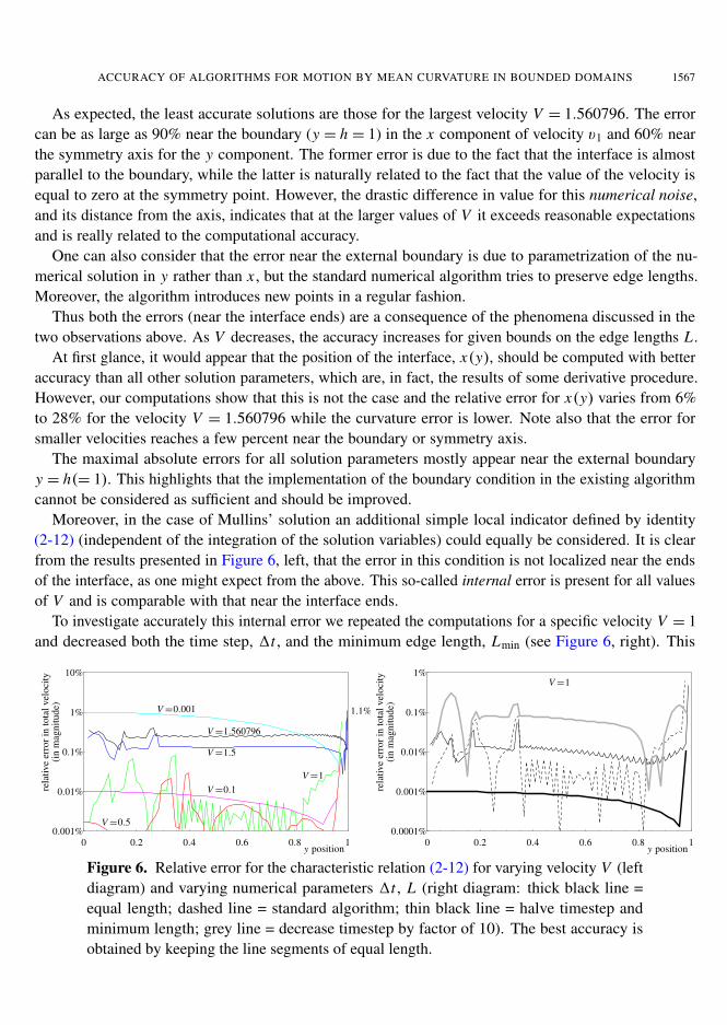
Moreover, in the case of Mullins’ solution an additional simple local indicator defined by identity(2-12) (independent of the integration of the solution variables) could equally be considered. It is clearfrom the results presented in Figure 6, left, that the error in this condition is not localized near the endsof the interface, as one might expect from the above. This so-called internal error is present for all valuesof V and is comparable with that near the interface ends.

To investigate accurately this internal error we repeated the computations for a specific velocity V = 1and decreased both the time step, 1t , and the minimum edge length, Lmin (see Figure 6, right). This

0 0.2 0.4 0.6 0.8 10.001%

0.01%

0.1%

1%

10%

y position

rela

tive

erro

rin

tota

lvel

ocity

(in

mag

nitu

de)

V=1.560796

1.1%

V=1.5

V=1

V=0.5

V=0.1

V=0.001

0 0.2 0.4 0.6 0.8 10.0001%

0.001%

0.01%

0.1%

1%V=1

y position

rela

tive

erro

rin

tota

lvel

ocity

(in

mag

nitu

de)

Figure 6. Relative error for the characteristic relation (2-12) for varying velocity V (leftdiagram) and varying numerical parameters 1t , L (right diagram: thick black line =equal length; dashed line = standard algorithm; thin black line = halve timestep andminimum length; grey line = decrease timestep by factor of 10). The best accuracy isobtained by keeping the line segments of equal length.

1568 SIMON COX AND GENNADY MISHURIS

has improved the quality of the computations, but there is still an error at some internal points of theinterval that is comparable with the error near the ends. Unfortunately the computational time increasesconsiderably. The obvious route of decreasing 1t but fixing Lmin, to ameliorate this effect, leads togreater error in the solution (see again Figure 6, right). The accuracy of the solution can be improvedinternally by making the line segments of equal length [Green et al. 2006]; although this doesn’t affectthe error at the boundary, it does make the calculations faster (see Figure 4).

Possible sources of internal error include: (a) nonoptimal distribution of the tessellation points alongthe interface after some time; (b) imperfections in the correction procedure (which adds and eliminatespoints from the interface at some prescribed time); and (c) point-to-point error variation related to thefact that the diffusion-type coefficient changes from point to point along the interface (recall that (2-1)is a nonlinear parabolic equation which is solved by a direct FD scheme with a fixed time step).

In the last computation in Figure 6, right, for the line segments of equal length, we have redistributedpoints to make the segments equal at every time step (note that this length may change in time). Apartfrom the fact that the number of tessellation points is smaller than for the standard algorithm, such acomparison is not absolutely fair as the redistribution in the standard algorithm (removing or subdividingedges with lengths outside the range 0.01≤ L ≤ 0.05) was done every 20 time steps. To discover if there

0 0.2 0.4 0.6 0.8 10.0001%

0.001%

0.01%

0.1%

1%

rela

tive

erro

rin

F(i

nm

agni

tude

)

tl1

tl20

tl20

V1

V20

0 0.2 0.4 0.6 0.8 10.001%

0.01%

0.1%

1%

10%

rela

tive

erro

rin

IF

(in

mag

nitu

de)

tl1tl20

V1

V20

0 0.2 0.4 0.6 0.8 10.001%

0.01%

0.1%

1%

10%

y position

rela

tive

erro

rin

Ir

(in

mag

nitu

de)

tl1

tl20V1

V20

0 0.2 0.4 0.6 0.8 10.001%

0.01%

0.1%

1%

10%

y position

rela

tive

erro

rin

Iv

(in

mag

nitu

de)

tl1, t120

V1, V20

Figure 7. Relative error in the computations shown by the integral measures for unitvelocity of the external boundary, V=1.0, obtained with four different computationalstrategies: the standard redistribution of the tessellation points, tl1 and tl20; and uniformlength segment redistribution, V1 and V20, at every time step and every twentieth step,respectively. The top left graph shows the function F of (2-24) (as in Figure 6); the otherthree graphs correspond to the three error indicators defined in (4-1)–(4-3). All integralswere computed with the trapezium rule.

ACCURACY OF ALGORITHMS FOR MOTION BY MEAN CURVATURE IN BOUNDED DOMAINS 1569

is an effect of redistribution frequency on the accuracy, we have tested these two algorithms under thesame strategy by redistributing the points (in a different way) every time step and every twentieth timestep. The error in the function F defined in (2-24), which is a constant in the case of the Mullinssolution, are presented in Figure 7, top left. It is evident that the standard algorithm is quite sensitive tothe chosen strategy. For a given position of the points on the interface, the relative error may differ byas much as two orders of magnitude, whereas this is not the case for the equal segment strategy. In thiscase, only near the external boundary is there some small fluctuation in the accuracy. Comparing thetwo redistribution algorithms for the same frequency of redistribution, the largest error always appearsin the case of the standard algorithm — by up to two orders of magnitude — despite the fact that thenumber of tessellation points was greater. Moreover, in the standard algorithm this error is irregularlydistributed along the interface. Recall that the number of tessellation points in the standard algorithmchanges during the computations from 25 initially to around 150 (for V = 1) in the steady-state regime,while the number of the points in the second (equal length) algorithm remains constant. Therefore thecomputational time for the second algorithm was less by a factor of approximately two. On the otherhand, the difference in the computational time between the different frequencies for redistribution forthe equal length algorithm was only a few percent. This indicates the further possibility of optimizingthis algorithm by redistributing points every MT time steps. It is clear that MT = MT (V ) and this needsfurther investigation [Green et al. 2006].

Note that the function F from (2-24) can be used as an indicator of the accuracy of the computationonly for the Mullins’ solution. However, there are three universal indicators which can be helpful toestimate the accuracy for any computations, namely, the relative errors of the numerical representationsof the identities (2-25), (2-27), and (2-30), embodied in the following explicit definitions:

After (2-25): IF =−

∫ y

0F(ξ)dξ ; relative error=

IF

θ(y)−π/2− 1. (4-1)

After (2-27): Ir =

∫ y

0

v2(ξ)

v1(ξ)dξ ; relative error=

Ir

x(0)− x(y)− 1. (4-2)

After (2-30): Iv =

∫ y

0v2(ξ)dξ ; relative error= Ir

/(v2

2(y)

2(v22(y)+ v

21(y))

)− 1. (4-3)

The respective results are shown in the remaining three parts of Figure 7. All four indicators suggestthat the equidistant distribution of the tessellation points is much better than the standard algorithm,regardless of the chosen strategy, as recommended in [Green et al. 2006]. Moreover, even near thesymmetry point, y = 0, where the value of the indicators all tend to zero and have a large influence onthe relative errors, the accuracy of the computations for the second algorithm is extremely high. However,this is not the case for the standard algorithm.

In Figure 8, the relative errors of the solution variables are presented for both algorithms: the standardone and the equidistant distribution. The result for x(y), shown in the top left part of the figure, lookssurprising at first glance; although the accuracy of the computations performed with these two algorithmsis of the same order and the error related to the new algorithm is distributed more uniformly, it appearsthat the accuracy of the standard algorithm is better than the equal-segment-length algorithm, at leastwith respect to the accuracy of the position of the interface. However, this is not the case. In fact, as

1570 SIMON COX AND GENNADY MISHURIS

was shown above, the computational error for the standard algorithm is redistributed along the interfaceirregularly whereas that for the equal-segment algorithm is practically uniform. As a result, the criterionto stop the iteration process to find the steady-state solution works differently for the two algorithms. Theprescribed maximal growth 10−8 in each time-step, measured on the axis of symmetry, is reached morequickly for the new algorithm. This is the second reason (together with number of tessellation points)why this algorithm is faster. If one were to run both algorithms for the same time, or for the same numberof iterations, and compare the corresponding results, the discussed paradox should not appear and thenew algorithm always provides better accuracy by as much as two orders of magnitude.

For the accuracy of other problem variables — the interface curvature, κ , and the interface velocities,v1 and v2 — the new algorithm is more accurate, notwithstanding the above argument, as can be seen inthe last three parts of Figure 8.

Finally, we stress again that the proposed three indicators are more versatile measures than a compar-ison of the numerical steady-state solution with the analytical one, since the latter comparison includesan additional error related to the determination of the steady-state regime, while the indicators show usaccuracy of the solution even if the steady state has not been reached.

5. Discussion and conclusions

All these results clearly indicate that the existing algorithm should be used with caution, especially wheninvestigating the behaviour of a many-bubble foam near the critical velocity. Moreover, when there

0 0.2 0.4 0.6 0.8 10.01%

0.1%

rela

tive

erro

rin

xpo

sitio

n(i

nm

agni

tude

)

tl1

tl20

V1V20

0 0.2 0.4 0.6 0.8 10.0001%

0.001%

0.01%

0.1%

1%

rela

tive

erro

rin

curv

atur

e(i

nm

agni

tude

)

tl1

tl20

V1, V20

0 0.2 0.4 0.6 0.8 10.0001%

0.001%

0.01%

0.1%

1%

y position

rela

tive

erro

rin

xve

loci

ty(i

nm

agni

tude

)

tl1

tl20

V1V1, V20

V20

0 0.2 0.4 0.6 0.8 10.0001%

0.001%

0.01%

0.1%

1%

10%

y position

rela

tive

erro

rin

yve

loci

ty(i

nm

agni

tude

)

tl1

tl20

V1V1, V20

V20

Figure 8. Relative error in the position x(y) of the interface (top left), its curvature κ(top right), and the x- and y- velocity components v1 and v2 (bottom row), for differentnumerical algorithms with velocity of the external boundary V=1.

ACCURACY OF ALGORITHMS FOR MOTION BY MEAN CURVATURE IN BOUNDED DOMAINS 1571

are many cells in a simulation (see Figure 3, right), the user is restricted to some critical number oftessellation points MP , which gives a limitation on accuracy even for low velocity. In fact, the materialstructure is highly nonuniform, in the sense that the cells may have different sizes. Effectively thismeans that every interface has its own critical velocity and the bigger cells thus introduce larger errors.In addition, it takes longer for curvature to diffuse along a longer interface and set it in motion. Thiscreates the following duality: to accurately describe the process of cell motion it is necessary to havethe computational error as small as possible, while the error generated near the critical velocity takes itsgreatest value. This is true for boundary or internal cells equally. Problems requiring high accuracy ofthe solution near the external boundary are related to the investigation of the boundary effects describingthe total phenomenological behaviour of the foam structures.

Another important remark is that the choice of the initial condition for testing the numerical procedurehere (a straight-line interface) is much more severe than any of the instantaneous solutions reported inSection 3. One could even think of worse situations to test the algorithm, for example if the initialinterface is not convex or even not smooth. This may lead to supercritical velocities and so on.

To revise and improve the existing numerical algorithm, we propose to use another strategy for theredistribution of the tessellation points: an equal-segment-length distribution of the tessellation points ismuch more favourable [Green et al. 2006]. However, this strategy is not sufficient to eliminate inaccuracyin the computation near the maximum velocity in the steady-state regime. The reason for this is thebehaviour of the steady-state solution near the wall (2-21). In fact, there exist two possible realizations ofthis algorithm. One, which we have used in our computations, is to keep the same number of tessellationpoints, MP , then with time the length between consecutive points, L , will increase significantly whenV is near Vcr. This leads to an effective loss of accuracy. Another strategy would be to keep the samedistance between points during the computations. However, MP will then increase to infinity as Vapproaches Vcr. Formally this should preserve computational accuracy but will lead to an unacceptableincrease in computational time and memory use. Thus, further adaptations to the algorithm are requiredif high accuracy is required, for example in the steady-state regime with velocities near the critical value[Cox 2005].

Taking advantage of the auxiliary identities (2-25), (2-27), and (2-30), we may correct the instanta-neous solution obtained within any algorithm at any or even every time step without time-consumingcomputations, as the identities are valid for any instantaneous solution. They also make possible furtherinvestigation of the asymptotic behaviour of the bounded interface solution near the ends. For example,any possible solution behaves at the symmetry axis according to (2-35), which allows us to tackle the errorin the solution near the symmetry axis. On the other hand, the results obtained in Section 2C may allowus to construct and implement a new numerical procedure/elements tackling the boundary condition in amore accurate way (without losing any near-boundary points, using, for example, a boundary layer result[Grassia et al. 2008]).

Finally, as we have shown, the identities (2-25), (2-27), and (2-30) may be used to probe the accuracyof computations. These indicators are extremely helpful as they are not based on information about theexact solution and can therefore illuminate inaccuracy of the numerical solution without any preliminaryknowledge about the exact solution itself.

Summarizing, we have shown that an improvement of the numerical algorithm is highly desirable andpossible. Apart from the fact that some of the improvements have been indicated and proven in this

1572 SIMON COX AND GENNADY MISHURIS

paper, there is still an open question how to deal with the accuracy of the computations near the criticalvelocities and near the external boundaries. We have also suggested possible directions for future inves-tigation: improved implementation of the boundary condition and creation of additional near-boundarypoints. Further, to check new results related to the numerical algorithm we need a larger set of analyticalbenchmarks.

Acknowledgements

The authors thank P. Grassia for his many helpful remarks on an earlier version, and the unknown refereesfor their insightful comments.

References

[Bragg and Nye 1947] L. Bragg and J. F. Nye, “A dynamical model of a crystal structure”, Proc. R. Soc. Lond. A 190:1023(1947), 474–481.

[Brakke 1992] K. Brakke, “The Surface Evolver”, Exp. Math. 1:2 (1992), 141–165.

[Cox 2005] S. J. Cox, “A viscous froth model for dry foams in the Surface Evolver”, Colloid. Surface. A 263:1–3 (2005),81–89.

[Grassia et al. 2008] P. Grassia, G. Montes-Atenas, L. Lue, and T. E. Green, “A foam film propagating in a confined geometry:analysis via the viscous froth model”, Eur. Phys. J. E 25:1 (2008), 39–49.

[Green et al. 2006] T. E. Green, A. Bramley, L. Lue, and P. Grassia, “Viscous froth lens”, Phys. Rev. E 74:5 (2006), 051403.

[Green et al. 2009] T. E. Green, P. Grassia, L. Lue, and B. Embley, “Viscous froth model for a bubble staircase structure underrapid applied shear: an analysis of fast flowing foam”, Colloid. Surface. A 348 (2009), 49–58.

[Kern et al. 2004] N. Kern, D. Weaire, A. Martin, S. Hutzler, and S. J. Cox, “Two-dimensional viscous froth model for foamdynamics”, Phys. Rev. E 70:4 (2004), 041411.

[Mullins 1956] W. W. Mullins, “Two-dimensional motion of idealized grain boundaries”, J. Appl. Phys. 27:8 (1956), 900–904.

[Peleg et al. 2001] A. Peleg, B. Meerson, and A. Vilenkin, “Area-preserving dynamics of a long slender finger by curvature: atest case for globally conserved phase ordering”, Phys. Rev. E 63:6 (2001), 066101.

[Smith 1952] C. S. Smith, “Grain shapes and other metallurgical applications of topology”, pp. 65–108 in Metal interfaces(Detroit, MI, 1951), American Society for Metals, Cleveland, OH, 1952.

[Weaire and Hutzler 1999] D. Weaire and S. Hutzler, The physics of foams, Clarendon, Oxford, 1999.

[Weaire and McMurry 1996] D. Weaire and S. McMurry, “Some fundamentals of grain growth”, Solid State Phys. 50 (1996),1–36.

[Wood 1996] G. P. Wood, Some problems in nonlinear diffusion, Ph.D. Thesis, University of Nottingham, 1996.

Received 14 Jan 2009. Revised 11 Mar 2009. Accepted 8 May 2009.

SIMON COX: foams@aber.ac.ukInstitute of Mathematics and Physics, Aberystwyth University, Aberystwyth SY23 3BZ, United Kingdom

GENNADY MISHURIS: ggm@aber.ac.ukInstitute of Mathematics and Physics and Wales Institute of Mathematical and Computational Sciences,Aberystwyth University, Aberystwyth SY23 3BZ, United Kingdom