Embed Size (px)
Citation preview

Mechanical Effects of Flow on CO2 Corrosion Inhibition of Carbon Steel Pipelines
A dissertation presented to
the faculty of
the Russ College of Engineering and Technology of Ohio University
In partial fulfillment
of the requirements for the degree
Doctor of Philosophy
Wei Li
August 2016
© 2016 Wei Li. All Rights Reserved.
2
This dissertation titled
Mechanical Effects of Flow on CO2 Corrosion Inhibition of Carbon Steel Pipelines
by
WEI LI
has been approved for
the Department of Chemical and Biomolecular Engineering
and the Russ College of Engineering and Technology by
Srdjan Nesic
Professor of Chemical and Biomolecular Engineering
Dennis Irwin
Dean, Russ College of Engineering and Technology
3
Abstract
LI, WEI, Ph.D., August 2016, Chemical Engineering
Mechanical Effects of Flow on CO2 Corrosion Inhibition of Carbon Steel Pipelines
Director of Dissertation: Srdjan Nesic
Transportation of multiphase fluids using carbon steel pipelines is ubiquitous in the
oil and gas industry. These pipelines are prone to internal corrosion when exposed to an
aqueous CO2 environment. The mitigation of CO2 corrosion can be achieved by the use
of organic corrosion inhibitors or by reliance on formation of protective corrosion
product layers. However, the mechanisms for their potential failure in flow conditions are
still being debated.
Wall shear stress induced by turbulent multiphase flow is considered an important
parameter in CO2 corrosion as it has been claimed to be responsible for the removal of
protective corrosion product layers and corrosion inhibitor films. In this study, a floating
element wall probe was used to directly measure the wall shear stresses in single-phase
and horizontal gas-liquid two-phase flow, instead of the more common indirect
measurement of the wall shear stress. Wall shear stress measurements were
complemented by high speed video camera recordings of the flow field. In single-phase
pipe and channel flow, the wall shear stress was in good agreement with empirical shear
stress calculations. In two-phase pipe flow, video-recorded observations confirmed that
the high wall shear stress pulses captured by the probe in the slug flow pattern were in
sync with the passage of liquid slugs; the highest measured wall shear stress values were
of the order of 100 Pa. Wall shear stress values in the slug body varied along the inner

4
pipe circumference with the top of the pipe having the highest values and the bottom of
the pipe having the lowest values. The maximum wall shear stress measured was about 2
to 4 times higher than the calculated mean wall shear stress in the slug body, obtained by
using the mixture velocity, which can serve as a guideline for slug flow modeling.
Findings suggest that the wall shear stress alone, produced in single-phase and
multiphase flow patterns covered in the present study, is insufficient to mechanically
damage the protective corrosion product layers or corrosion inhibitor films.
In addition, corrosion experiments with an imidazoline-based inhibitor were
performed on X65 pipeline steel in a thin channel flow cell (TCFC). Local flow velocities
were up to 28 m/s with wall shear stresses up to 4.8 kPa. Electrochemical measurements,
surface analysis and computational fluid dynamics (CFD) were used as diagnostic tools.
Localized corrosion was observed on a protrusion in the flow cell and depended on local
flow conditions and inhibitor concentration. Overall, the wall shear stress was unable to
affect performance of corrosion inhibitors. However, the low static pressure at the
protrusion caused cavitation with bubble collapse leading to accelerated desorption of
inhibitor from the steel surface, which explained the localized corrosion. An excess
amount of inhibitor was found to mitigate localized corrosion by cavitation.

5
Dedication
To my love, my family and my friends.

6
Acknowledgments
I am indebted to many individuals who have helped me during my PhD journey,
personally and professionally. First and foremost, I would like to express my genuine
gratitude to my advisor, Dr. Srdjan Nesic, for his academic advice and constant support
throughout my entire graduate studies. His dedication and energy to research and life
serve as my role model and will continue to inspire me, which would be my lifelong
fortune.
Many thanks also go to my dissertation committee members, Drs. David Young,
Yoon-Seok Choi, Marc Singer, Douglas Green and Lauren McMills for their academic
assistance and time.
I am deeply grateful to my mentors, Drs. B.F.M. Pots, Luciano Paolinelli and
Sumit Sharma for their invaluable advice and discussion related to my research.
Thank you to all members of the Institute for Corrosion and Multiphase Technology.
Particularly, I would like to thank my research group leader, Dr. Bruce Brown, for his
technical support and constant availability during my research program. Thank you to the
technical staff for their support during my experimental research, especially
Alexis Barxias, Daniel Cain, Phil Bullington and Cody Shafer. Thanks to Becky Gill for
administrative support.
Many thanks go to my fellow colleagues at the institute for their help and support. I
particularly thank Drs. Kok Eng Kee, Channa De Silva and Xiankang Zhong for their
help with my experimental work. In addition, I would like to acknowledge

7
Dr. Fardis Najafifard, Dr. Baotang Zhuang, Dr. Haijun Hu and Yingrodge Suntiwuth for
their assistance on computer simulation.
Thank you to Dr. David Young and Lisa Mosier for their help in proofreading for this
dissertation.
Finally, I am indebted to my parents, my love and other family members for their
support, encouragement, prayers and patience throughout my long journey of pursuing
graduate studies.

8
Table of Contents
Page
Abstract ............................................................................................................................... 3
Dedication ........................................................................................................................... 5
Acknowledgments............................................................................................................... 6
List of Tables .................................................................................................................... 12
List of Figures ................................................................................................................... 13
List of Abbreviations ........................................................................................................ 20
Chapter 1: Introduction ..................................................................................................... 23
Chapter 2: Background and Literature Review ................................................................ 27
2.1 Basics of CO2 Corrosion ........................................................................................ 27
2.1.1 CO2 corrosion mechanisms ........................................................................... 28
2.1.2 Mitigation of CO2 corrosion .......................................................................... 30
2.2 Flow Patterns in Gas-Liquid Two-Phase Flow ...................................................... 39
2.3 Effects of Flow on Mitigation of CO2 Corrosion ................................................... 42
2.3.1 Effect of mass transfer ................................................................................... 43
2.3.2 Effect of mechanical forces ........................................................................... 45
2.3.3 Other miscellaneous effects found in multiphase flow ................................. 48
2.4 Wall Shear Stress Measurements ........................................................................... 49
2.4.1 Direct measurements ..................................................................................... 49
2.4.2 Indirect measurements ................................................................................... 53
Chapter 3: Research Objectives ........................................................................................ 59
Chapter 4: Experimental Methodology ............................................................................. 61
4.1 Physical Measurement of Wall Shear Stress .......................................................... 61
9
4.2 Instrumentation and Methods for Flow Tests......................................................... 64
4.2.1 Equipment for single-phase flow .................................................................. 64
4.2.2 Equipment for gas-liquid two-phase flow ..................................................... 67
4.2.3 Equipment for flow visualization .................................................................. 68
4.2.4 Computational fluid dynamics (CFD) ........................................................... 69
4.3 Electrochemical Characterization Techniques for Corrosion Tests ....................... 69
4.4 Techniques for Surface Characterization ............................................................... 70
Chapter 5: Direct Wall Shear Stress Measurements in Gas-Liquid Two-Phase Flow ..... 71
5.1 Introduction ............................................................................................................ 71
5.2 Experimental Methodology .................................................................................... 71
5.3 Wall Shear Stress Measurements in Single-Phase Flow ........................................ 74
5.4 Wall Shear Stress Measurements in Gas-Liquid Two-Phase Horizontal Pipe Flow ...................................................................................................................................... 80
5.4.1 Wall shear stress measurements in slug flow ................................................ 80
5.4.2 Assessment of the location with the highest wall shear stress in a slug ........ 98
5.4.3 Determination of slug frequency ................................................................. 101
5.4.4 Wall shear stress measurements in stratified flow and annular flow .......... 106
5.5 Discussion ............................................................................................................ 109
5.6 Summary .............................................................................................................. 112
Chapter 6: Mechanical Effects of Flow on CO2 Corrosion Inhibition............................ 114
6.1 Introduction .......................................................................................................... 114
6.2 Experimental ........................................................................................................ 114
6.2.1 Flow system for corrosion tests ................................................................... 114
6.2.2 Corrosion specimens ................................................................................... 115

10
6.2.3 Experimental procedures ............................................................................. 119
6.3 Experimental Results ............................................................................................ 122
6.3.1 Corrosion tests without inhibitor ................................................................. 122
6.3.2 Corrosion tests with inhibitor ...................................................................... 127
6.3.3 Effect of oxygen ingress on corrosion inhibition ........................................ 134
6.3.4 Effect of wall shear stress on corrosion inhibition ...................................... 142
6.3.5 Effect of cavitation on corrosion inhibition ................................................ 145
6.3.6 Mitigation of cavitation induced localized corrosion .................................. 151
6.4 Discussion ............................................................................................................ 157
6.4.1 Effect of pre-corrosion on corrosion inhibition at high flow velocity ........ 158
6.4.2 B value at high flow velocity ...................................................................... 158
6.4.3 Mechanisms of flow cavitation induced pitting corrosion and its mitigation .............................................................................................................................. 160
6.4.4 Microscopic expressions for continuum hydrodynamics ............................ 170
6.5 Summary .............................................................................................................. 171
Chapter 7: Conclusions and Recommendations ............................................................. 173
7.1 Conclusions .......................................................................................................... 173
7.2 Recommendations ................................................................................................ 175
References ....................................................................................................................... 177
Appendix 1. Measurement of the Mass Transfer Limiting Current Using the Ferricyanide-Ferrocyanide Couple ....................................................................................................... 191
Appendix 2. Procedures for Calibrating the Paddlewheel Flow Meter and the Orifice Plate Flow Meter ............................................................................................................. 193
Appendix 3. Calculation of Corrosion Rate by Weight Loss and Linear Polarization Resistance ....................................................................................................................... 196

11
Appendix 4. Calculation of the Absolute Pressure at the Inlet of the CFD Simulation for Protrusion in the Thin Channel Flow Cell ...................................................................... 198

12
List of Tables
Page
Table 2-1: Key chemical reactions of aqueous CO2 corrosion and the corresponding chemical equilibrium expressions ..................................................................................... 29
Table 2-2: Key electrochemical reactions of aqueous CO2 corrosion .............................. 29
Table 2-3: Chemical formulation of the model inhibitor K1 [wt.%] ................................ 39
Table 4-1: Typical parameter settings for electrochemical measurements ....................... 70
Table 5-1: Test matrix for single-phase flow .................................................................... 73
Table 5-2: Test matrix for gas-liquid two-phase flow ...................................................... 73
Table 5-3: Wall shear stress measurements for slug flow in the 4 inch pipe loop ........... 85
Table 5-4: Maximum local liquid velocity (Vmax) calculated from the video data in the slug body, for 4 inch pipe loop ......................................................................................... 95
Table 5-5: Selected empirical correlations for slug frequency determination [82,84,85]......................................................................................................................................... 104
Table 5-6: Error statistics for slug frequency: (predicted – measured)/measured, for the data produced by using different empirical correlations ................................................. 105
Table 5-7: WSS data measured for annular flow at the bottom and on the side wall of the 6 inch pipe ....................................................................................................................... 109
Table 6-1: Chemical analysis [wt.%] of API 5L X65 carbon steel ................................ 116
Table 6-2: Test matrix for corrosion inhibition test with high flow velocity ................. 120

13
List of Figures
Page
Figure 2-1: A top view SEM image of a steel surface covered by a FeCO3 layer. 80oC, 0.53 bar CO2, pH 7.8, stagnant. ........................................................................................ 32
Figure 2-2: A cross-sectional side view TEM image of a FeCO3 covered steel surface. 80oC, 0.53 bar CO2, pH 7.1, stagnant. The specimen was coated with Au and Pt during specimen preparation. ....................................................................................................... 32
Figure 2-3: Adsorption mechanisms of ionic surfactants on the charged substrate surface (adapted from [54]). .......................................................................................................... 37
Figure 2-4: Curve of surface tension – surfactant concentration. ..................................... 37
Figure 2-5: Molecular structure of TOFA/DETA imidazolinium ion. ............................. 39
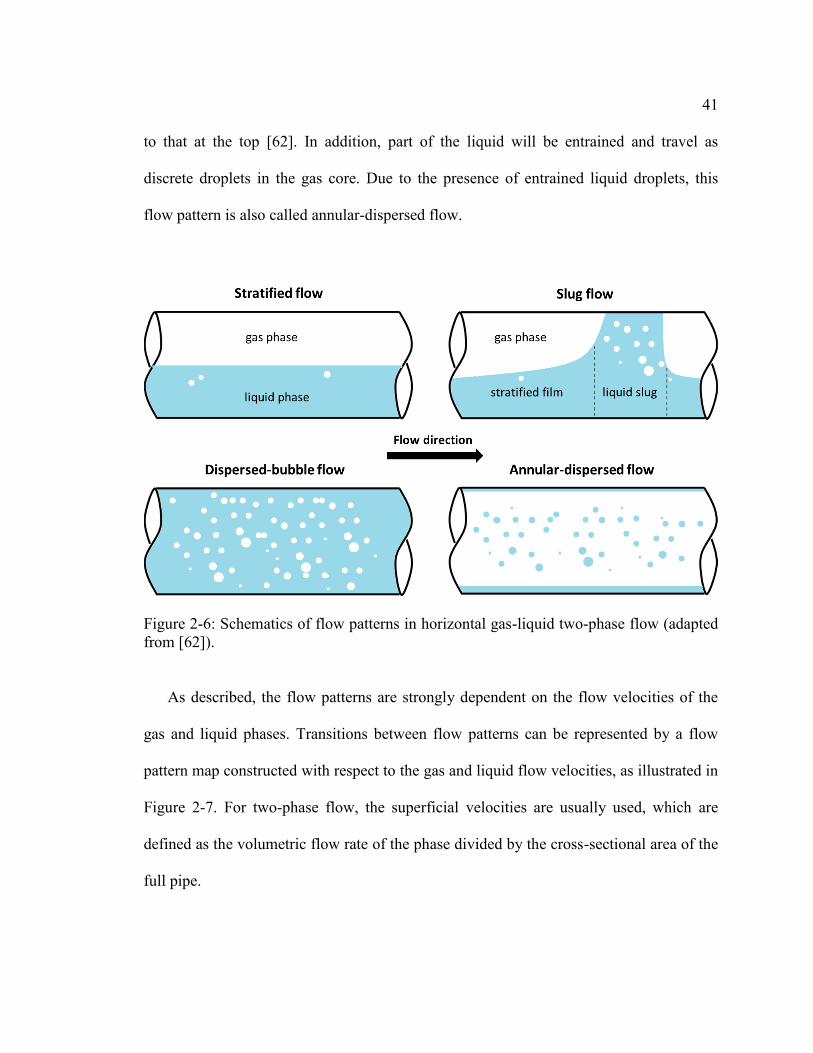
Figure 2-6: Schematics of flow patterns in horizontal gas-liquid two-phase flow (adapted from [62]). ......................................................................................................................... 41
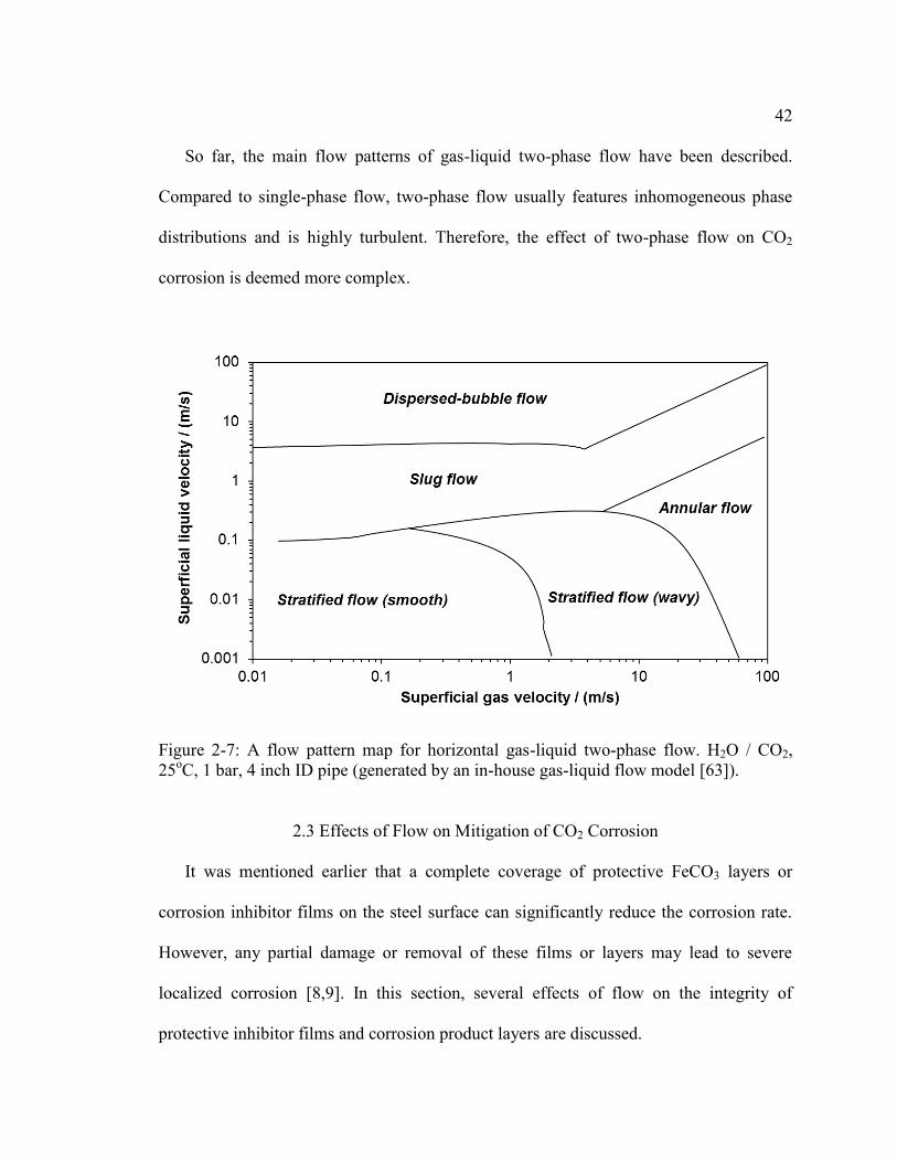
Figure 2-7: A flow pattern map for horizontal gas-liquid two-phase flow. H2O / CO2, 25oC, 1 bar, 4 inch ID pipe (generated by an in-house gas-liquid flow model [63]). ....... 42
Figure 2-8: Potentiodynamic polarization curves measuring the mass transfer limiting currents of the ferri/ferrocyanide. Nickel RCE electrode (a diameter of 12 mm and length of 14 mm), 25oC, 2 M NaOH, 0.01 M K4[Fe(CN)6] / K3[Fe(CN)6], 1 bar N2. ................. 44
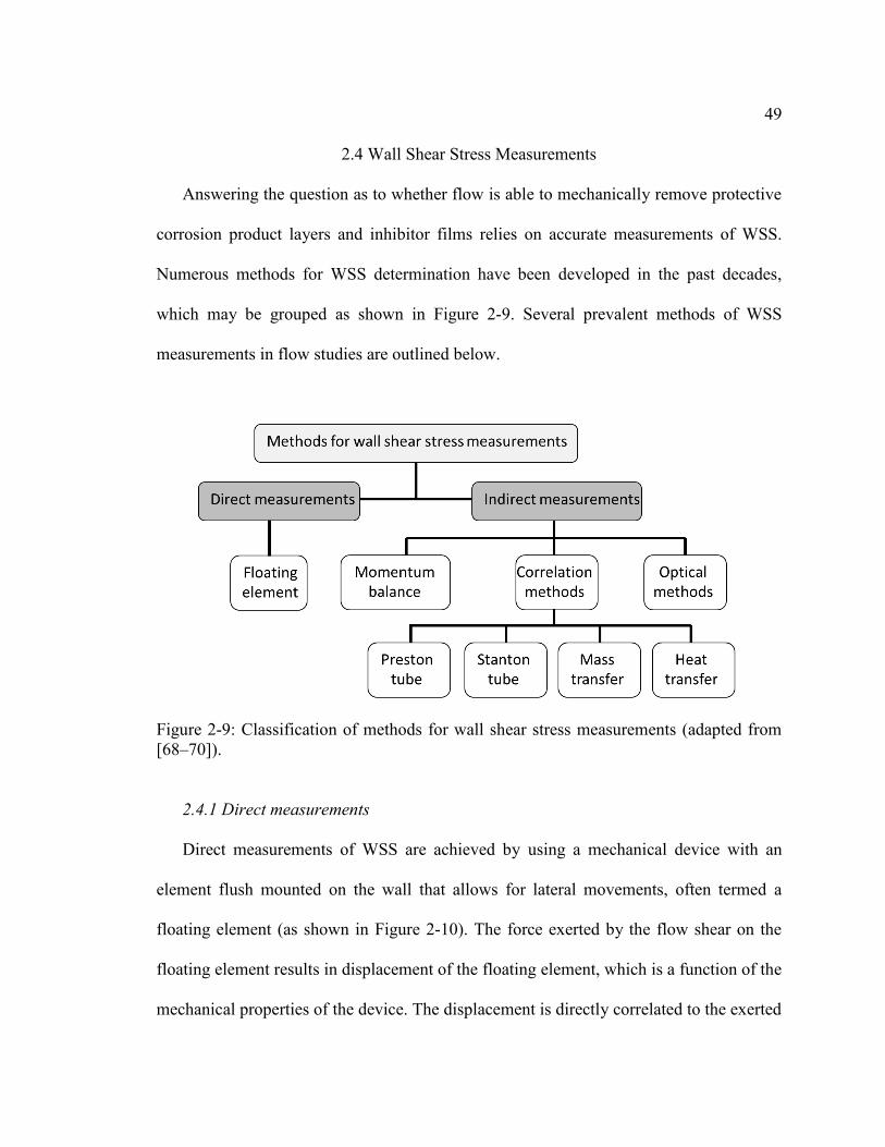
Figure 2-9: Classification of methods for wall shear stress measurements (adapted from [68–70])............................................................................................................................. 49
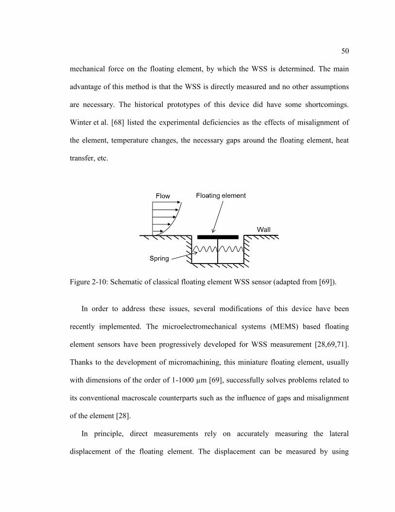
Figure 2-10: Schematic of classical floating element WSS sensor (adapted from [69]). . 50
Figure 2-11: Schematic of heat or mass transfer WSS sensor (adapted from [28]). ........ 55
Figure 2-12: Schematic of laser-based WSS sensor (adapted from [70]). ........................ 57
Figure 4-1: (A) Schematic of a floating element WSS measurement system showing sample measurement; (B) schematic diagram of WSS probe body (by Lenterra with permission). ....................................................................................................................... 62
Figure 4-2: Visual representations of: (A) thin channel flow cell assembly and (B) zoomed-in view of the bottom plate of the test section (top lid not shown). .................... 65
Figure 4-3: Representation of 10.2 cm ID (4 inch) pipe flow loop. ................................. 66
14
Figure 4-4: Schematic of the WSS probe holder flush-mounted to the pipe wall. ........... 67
Figure 4-5: Representation of 15.2 cm ID (6 inch) once-through pipe system. ............... 68
Figure 5-1: Tested flow conditions for WSS measurements in a horizontal two-phase flow pattern map [63] for 1 bar, 25oC, CO2-water, and 4-inch pipe loop. ........................ 74
Figure 5-2: Comparison of measured WSS values with Patel calculations for channel flow (h=3 mm). ................................................................................................................. 76
Figure 5-3: Comparison of measured WSS values with calculations for pipe flow (ID=0.102 m). ................................................................................................................... 76
Figure 5-4: ANSYS geometry for the test section of the thin channel flow cell. ............. 78
Figure 5-5: Mesh structure in the thin channel flow cell, a view from z-direction. ......... 78
Figure 5-6: WSS distribution at the port locations by CFD simulation. 25oC, 9.5 m/s in the thin channel flow cell. ................................................................................................. 79
Figure 5-7: Comparison of WSS values obtained by different methods. ......................... 79
Figure 5-8: Wall shear stress measurement at the bottom of the 4 inch pipe for Vsl =2.0 m/s, Vsg = 2.1 m/s: (A) the full recording sequence; (B) data between 32 and 38 seconds (See Figure 5-20 for the synchronized video frames of the labeled peaks). ..................... 82
Figure 5-9: Wall shear stress measurement at the top of the 4 inch pipe loop for Vsl = 2.0 m/s, Vsg = 2.6 m/s: (A) the full recording sequence; (B) data between 70 and 80 seconds (See Figure 5-21 and Figure 5-22 for the synchronized video frames of the labeled peaks).................................................................................................................... 82
Figure 5-10: Wall shear stress measurement at the sidewall of the 4 inch pipe loop for Vsl = 0.3 m/s, Vsg = 2.6 m/s: (A) the full recording sequence; (B) data between 160 and 200 seconds. ...................................................................................................................... 83
Figure 5-11: 𝜏max (Pa) shown next to markers for slug flow measured at the bottom of the pipe overlain with the flow pattern map [63], at 1 bar, 25oC, CO2-water, and in the 4-inch loop. .................................................................................................................................. 86
Figure 5-12: 𝜏max (Pa) shown next to markers for slug flow measured at the top of the pipe overlain with the flow pattern map [63], at 1 bar, 25oC, CO2-water, and in the 4-inch loop. .................................................................................................................................. 86
Figure 5-13: 𝜏max (Pa) shown next to markers for slug flow measured at the sidewall overlain with the flow pattern map [63], at 1 bar, 25oC, CO2-water, and in the 4-inch loop. .................................................................................................................................. 87
15
Figure 5-14: Comparison between measured maximum WSS values and calculated mean slug WSS values from Equation (5-12) by using mixture velocity (Vm), for 4-inch loop.89
Figure 5-15: Illustration of calculating the in situ liquid velocities in a slug body. Time difference between frames Δt = 0.003 s. Vsl=1.0 m/s, Vsg= 0.6 m/s. ................................ 91
Figure 5-16: Illustration of tracking the tracer in the video frame at t = Δt...................... 93
Figure 5-17: Illustration of tracking the tracer in two video frames using the cross correlation method. (A): the matrix A containing the tracer in grayscale at t = 0 s (marked by blue rectangle in Figure 5-15); (B) the calculated correlation coefficients between the matrix A and the moving matrix B; (C) the moving matrix B with the maximum correlation to matrix A in grayscale at t = 0.003 s. ........................................................... 94
Figure 5-18: Comparison between maximum local liquid velocity (Vmax) in the slug body calculated from the video data and the mixture velocity (Vm) at each flow condition, for 4 inch pipe loop. ................................................................................................................... 96
Figure 5-19: Comparison between measured maximum WSS values and calculated maximum slug WSS values from Equation (5-12) by using Vmax from the video data, for 4 inch pipe loop. ................................................................................................................ 97
Figure 5-20: Video frames of slug passages corresponding to the three WSS measurement peaks marked in Figure 5-8(B), Vsl = 2.0 m/s, Vsg = 2.1 m/s: 1. the WSS probe is at the pipe bottom; 2. a scale tape of 2 cm long. ........................................................................ 99
Figure 5-21: Evolution of the WSS fluctuations with synchronized video frames of the slug around 74.29 s marked in Figure 5-9(B), Vsl = 2.0 m/s, Vsg = 2.6 m/s, 4 inch pipe.......................................................................................................................................... 100
Figure 5-22: Video frames of slug passages corresponding to the three WSS measurement peaks marked in Figure 5-9(B), Vsl = 2.0 m/s, Vsg = 2.6 m/s: 1. the WSS probe is at the pipe top; 2. a scale tape of 2 cm long. ............................................................................. 101
Figure 5-23: Comparison of measured slug frequencies by different methods (video data: hollow markers; WSS data: solid black markers) with the data of Heywood and Richardson (1979) [82] (solid gray markers).................................................................. 103
Figure 5-24: Comparison of measured slug frequencies with the Heywood correlation: (A) using the pipe diameter of this study; (B) using the pipe diameter of 42 mm. ........ 106
Figure 5-25: Wall shear stress measurement at the bottom of the 4 inch pipe for stratified flow at Vsl = 0.1 m/s, Vsg = 6.1 m/s: (A) the full recording sequence; (B) a typical video frame at this condition. ................................................................................................... 107
16
Figure 5-26: Wall shear stress measurement at the bottom of the 6 inch pipe for annular flow at Vsl = 0.2 m/s, Vsg = 42.2 m/s: (A) the full recording sequence; (B) a typical video frame at this condition (1: the WSS probe location; 2: a scale tape of 2 cm long). ........ 108
Figure 6-1: Specification and flow orientation for flat weight loss specimens. Left: side view; right: top view. ...................................................................................................... 116
Figure 6-2: Specification and flow orientation of Specimen 3, protrusion weight loss specimen: left: side view; right: top view. ...................................................................... 117
Figure 6-3: Configuration of the electrochemical probe. ................................................ 118
Figure 6-4: Location arrangement of the specimens in the TCFC.................................. 119
Figure 6-5: LPR corrosion rate for blank test, B = 65 mV. 1 wt.% NaCl, pH 5, 0.97 bar CO2, 25oC, 16 m/s, API 5L X65 carbon steel, 4 ppb to 30 ppb O2................................. 124
Figure 6-6: Profilometry results of protrusion Specimen 3 after the blank test. A: contour of the surface depth; B: line pattern depth scan of the surface marked by the red straight line in A. 1 wt.% NaCl, pH 5, 0.97 bar CO2, 25oC, 16 m/s, 4 day, X65, 4 ppb to 30 ppb O2. ................................................................................................................................... 125
Figure 6-7: SEM images of protrusion Specimen 3 after the blank test. Frist row: 50X magnification; second row: 1000X magnification. Physical locations are defined by using 5 numbered individual regions in Figure 6-2. 1 wt.% NaCl, pH 5, 0.97 bar CO2, 25oC, 16 m/s, 4 day test duration, X65, 4 ppb to 30 ppb O2. .................................................... 126
Figure 6-8: EDS analysis of flat Specimen 2 (150 grit) after the blank test. 1 wt.% NaCl, pH 5, 0.97 bar CO2, 25oC, 16 m/s, 4 day, X65, 4 ppb to 30 ppb O2. .............................. 127
Figure 6-9: LPR corrosion rate for blank and 72 ppmv TOFA imidazoline inhibitor tests, B = 65 mV. 1wt.% NaCl, pH 5, 0.97 bar CO2, 25oC, 16 m/s, 4 day test duration, X65, 4 ppb to 30 ppb O2. ............................................................................................................ 128
Figure 6-10: SEM images of flat Specimen 1 (600 grit finish) and Specimen 2 (150 grit finish) at 1000X magnification. 1 wt.% NaCl, pH 5, 0.97 bar CO2, 25oC, 72 ppmv inhibitor, 16 m/s, 4 day test duration, X65, 4 ppb to 30 ppb O2: A. Specimen 1 before test; B. Specimen 1 after test; C. Specimen 2 before test; D. Specimen 2 after test....... 129
Figure 6-11: Profilometry results of flat Specimen 1 (600 grit finish) after the test. A: contour of the surface depth; B: line pattern depth scan of the surface marked by the red straight line in A.............................................................................................................. 130
Figure 6-12: Profilometry results of flat Specimen 2 (150 grit finish) after the test. A: contour of the surface depth; B: line pattern depth scan of the surface marked by the red straight line in A.............................................................................................................. 130

17
Figure 6-13: SEM images of protrusion Specimen 3. Before test: 1st row at 50X magnification. After test: 2nd row at 50X magnification; 3rd row at 1000X magnification. Physical locations are defined by using 5 numbered individual regions in Figure 6-2. 1 wt.% NaCl, pH 5, 0.97 bar CO2, 25oC, 72 ppmv inhibitor, 16 m/s, 4 day test duration, X65, 4 ppb to 30 ppb O2. ................................................................................. 131
Figure 6-14: (A): Profilometry image of protrusion Specimen 3 after experiment on the top of protrusion, region 3 in Figure 6-2; (B): line pattern depth scan of the dotted red line marked in (A). 1 wt.% NaCl, pH 5, 0.97 bar CO2, 25oC, 72 ppmv inhibitor, 16 m/s, 4 day test duration, X65, 4 ppb to 30 ppb O2. .......................................................................... 132
Figure 6-15: EDS analysis of protrusion Specimen 3 after test on the top of protrusion, region 3 in Figure 6-2. A: inside a pit; B. the surrounding flat area above the pit. ........ 133
Figure 6-16: LPR corrosion rate for 72 ppmv inhibitor tests with varied levels of O2 concentration, B = 65 mV. 1 wt.% NaCl, pH 5, 0.97 bar CO2, 25oC, 16 m/s, 4 day test duration, X65. ................................................................................................................. 135
Figure 6-17: SEM images of flat Specimen 1 (600 grit finish) and Specimen 2 (150 grit finish) at 1000X magnification. 1 wt.% NaCl, pH 5, 0.97 bar CO2, 25oC, 72 ppmv inhibitor, 16 m/s, 4 day test duration, X65, O2 < 2 ppb: A. Specimen 1 before test; B. Specimen 1 after test; C. Specimen 2 before test; D. Specimen 2 after test. .................. 136
Figure 6-18: SEM images of protrusion Specimen 3. Before test: 1st row at 50X magnification. After test: 2nd row at 50X magnification; 3rd row at 1000X magnification. Physical locations are defined by using 5 numbered individual regions in Figure 6-2. 1 wt.% NaCl, pH 5, 0.97 bar CO2, 25oC, 72 ppmv inhibitor, 16 m/s, 4 day test duration, X65, O2 < 2 ppb. .............................................................................................. 137
Figure 6-19: (A): Profilometry image of protrusion Specimen 3 after experiment on top of protrusion, region 3 in Figure 6-2; (B): line pattern depth scan marked by the dotted red line in (A). 1 wt.% NaCl, pH 5, 0.97 bar CO2, 25oC, 72 ppmv inhibitor, 16 m/s, 4 day test duration, X65, O2 < 2 ppb. ....................................................................................... 138
Figure 6-20: EDS analysis of flat Specimen 1 (600 grit finish). A: before experiment; B. after experiment. 1 wt.% NaCl, pH 5, 0.97 bar CO2, 25oC, 72 ppmv inhibitor, 16 m/s, 4 day test duration, X65, O2 < 2 ppb. ................................................................................ 139
Figure 6-21: EDS analysis of flat Specimen 2 (150 grit finish). A: before experiment; B. after experiment. 1 wt.% NaCl, pH 5, 0.97 bar CO2, 25oC, 72 ppmv inhibitor, 16 m/s, 4 day test duration, X65, O2 < 2 ppb. ................................................................................ 140
Figure 6-22: EDS analysis of protrusion Specimen 3. A: before experiment; B. after experiment, in a pit at the top of protrusion, region 3 in Figure 6-2. 1 wt.% NaCl, pH 5, 0.97 bar CO2, 25oC, 72 ppmv inhibitor, 16 m/s, 4 day test duration, X65, O2 < 2 ppb. . 141
18
Figure 6-23: Schematic of the CFD simulation geometry with the symmetric plane outlined (red lines). ......................................................................................................... 142
Figure 6-24: Flow velocity magnitude distribution on the symmetric plane. ................. 144
Figure 6-25: Wall shear stress distribution at the bottom plate of the TCFC near the specimen protrusion. ....................................................................................................... 144
Figure 6-26: Wall shear stress distribution: A. on the symmetric plane; B. on the bottom wall of the symmetric plane. ........................................................................................... 145
Figure 6-27: Gauge pressure distribution: A. on the symmetric plane; B. on the bottom wall of the symmetric plane. ........................................................................................... 146
Figure 6-28: LPR corrosion rate for 72 ppmv inhibitor tests with changes of the protrusion specimen location, B = 65 mV. 1 wt.% NaCl, pH 5, 0.97 bar CO2, 25oC, 16 m/s, 4 day test duration, X65, O2 < 2 ppb. ....................................................................................... 149
Figure 6-29: SEM images of flat Specimen 1 (600 grit finish) at 1000X magnification. 1 wt.% NaCl, pH 5, 0.97 bar CO2, 25oC, 72 ppmv inhibitor, 16 m/s, 4 day test duration, X65, O2 < 2ppb: A. Specimen 1 before test; B. Specimen 1 after test. .......................... 149
Figure 6-30: SEM images of protrusion Specimen 3 on the most upstream port in the TCFC (port 1). Before test: 1st row at 50X magnification. After test: 2nd row at 50X magnification; 3rd row at 1000X magnification. Physical locations are defined by using 5 numbered individual regions in Figure 6-2. 1 wt.% NaCl, pH 5, 0.97 bar CO2, 25oC, 72 ppmv inhibitor, 16 m/s, 4 day test duration, X65, O2 < 2 ppb. .................................. 150
Figure 6-31: LPR corrosion rate for 720 ppmv inhibitor test, B = 65 mV. 1 wt.% NaCl, pH 5, 0.97 bar CO2, 25oC, 16 m/s, 4 day test duration, X65. ......................................... 152
Figure 6-32: SEM images of flat Specimen 1 (600 grit finish) and Specimen 2 (150 grit finish) at 1000X magnification. 1 wt.% NaCl, pH 5, 0.97 bar CO2, 25oC, 720 ppmv inhibitor, 16 m/s, 4 day test duration, X65, O2 < 2ppb: A. Specimen 1 before test; B. Specimen 1 after test; C. Specimen 2 before test; D. Specimen 2 after test. .................. 152
Figure 6-33: SEM images of protrusion Specimen 3. Before test: 1st row at 50X magnification. After test: 2nd row at 50X magnification; 3rd row at 1000X magnification. Physical locations are defined by using 5 numbered individual regions in Figure 6-2. 1 wt.% NaCl, pH 5, 0.97 bar CO2, 25oC, 720 ppmv inhibitor, 16 m/s, 4 day test duration, X65, O2 < 2 ppb. ....................................................................................... 153
Figure 6-34: EDS analysis of flat Specimen 1 (600 grit finish). A: before experiment; B. after experiment. 1 wt.% NaCl, pH 5, 0.97 bar CO2, 25oC, 720 ppmv inhibitor, 16 m/s, 4 day test duration, X65, O2 < 2 ppb. ............................................................................. 154
19
Figure 6-35: EDS analysis of protrusion Specimen 3. A: before experiment; B. after experiment, at the top of protrusion, region 3 in Figure 6-2. 1 wt.% NaCl, pH 5, 0.97 bar CO2, 25oC, 720 ppmv inhibitor, 16 m/s, 4 day test duration, X65, O2 < 2 ppb. .............. 155
Figure 6-36: Pressure drop measurements between port 3 and port 4 in the TCFC with various inhibitor concentrations. 1 wt.% NaCl, pH 5, 0.97 bar CO2, 25oC. ................... 157
Figure 6-37: Corrosion rates calculated from averaged weight losses of specimens and from LPR corrosion rate curves with B = 65 mV. 1 wt.% NaCl, pH 5, 0.97 bar CO2, 25oC, 16 m/s, 4 day test duration, X65. .......................................................................... 160
Figure 6-38: Energy diagram of inhibitor adsorption/desorption reactions. ................... 165
Figure 6-39: Energy diagram of inhibitor adsorption/desorption reactions with the additional energy due to collapsing cavitation bubbles. ................................................. 168

20
List of Abbreviations
AFM Atomic force microscopy
AISI American Iron and Steel Institute
AOPL Association of Oil Pipe Lines
API American Petroleum Institute
CAS Chemical Abstracts Service
CE Counter electrode
CFD Computational fluid dynamics
CMC Critical micelle concentration
CO2-EOR Carbon dioxide enhanced oil recovery
CR Corrosion rate
DI water Deionized water
DNS Direct numerical simulation
EDS Energy-dispersive X-ray spectroscopy
EIS Electrochemical impedance spectroscopy
FBG Fiber Bragg grating
fps Frames per second

21
ID Internal diameter
LPR Linear polarization resistance
MD Molecular dynamics simulation
MEMS Microelectromechanical systems
OCP Open circuit potential
OD Outer diameter
PDP Potentiodynamic polarization
ppb Part per billion (109), by weight
ppmv Part per million (106), by volume
PR Penetration rate
PVC Polyvinyl chloride
RCE Rotating cylinder electrode
RE Reference electrode
SEM Scanning electron microscopy
TCFC Thin channel flow cell
TEM Transmission electron microscopy
TLC Top-of-the-line corrosion

22
TOFA/DETA Tall oil fatty acid / diethylenetriamine
UDC Under-deposit corrosion
WE Working electrode
WSS Wall shear stress
ZRA Zero resistance ammeter
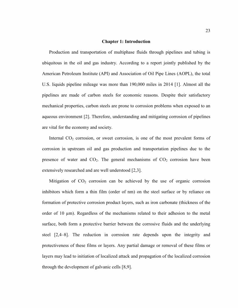
23
Chapter 1: Introduction
Production and transportation of multiphase fluids through pipelines and tubing is
ubiquitous in the oil and gas industry. According to a report jointly published by the
American Petroleum Institute (API) and Association of Oil Pipe Lines (AOPL), the total
U.S. liquids pipeline mileage was more than 190,000 miles in 2014 [1]. Almost all the
pipelines are made of carbon steels for economic reasons. Despite their satisfactory
mechanical properties, carbon steels are prone to corrosion problems when exposed to an
aqueous environment [2]. Therefore, understanding and mitigating corrosion of pipelines
are vital for the economy and society.
Internal CO2 corrosion, or sweet corrosion, is one of the most prevalent forms of
corrosion in upstream oil and gas production and transportation pipelines due to the
presence of water and CO2. The general mechanisms of CO2 corrosion have been
extensively researched and are well understood [2,3].
Mitigation of CO2 corrosion can be achieved by the use of organic corrosion
inhibitors which form a thin film (order of nm) on the steel surface or by reliance on
formation of protective corrosion product layers, such as iron carbonate (thickness of the
order of 10 µm). Regardless of the mechanisms related to their adhesion to the metal
surface, both form a protective barrier between the corrosive fluids and the underlying
steel [2,4–8]. The reduction in corrosion rate depends upon the integrity and
protectiveness of these films or layers. Any partial damage or removal of these films or
layers may lead to initiation of localized attack and propagation of the localized corrosion
through the development of galvanic cells [8,9].
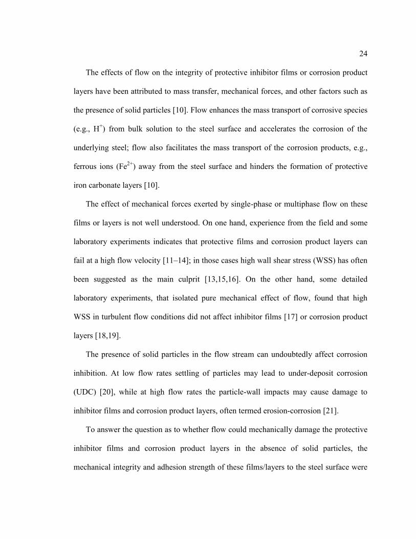
24
The effects of flow on the integrity of protective inhibitor films or corrosion product
layers have been attributed to mass transfer, mechanical forces, and other factors such as
the presence of solid particles [10]. Flow enhances the mass transport of corrosive species
(e.g., H+) from bulk solution to the steel surface and accelerates the corrosion of the
underlying steel; flow also facilitates the mass transport of the corrosion products, e.g.,
ferrous ions (Fe2+) away from the steel surface and hinders the formation of protective
iron carbonate layers [10].
The effect of mechanical forces exerted by single-phase or multiphase flow on these
films or layers is not well understood. On one hand, experience from the field and some
laboratory experiments indicates that protective films and corrosion product layers can
fail at a high flow velocity [11–14]; in those cases high wall shear stress (WSS) has often
been suggested as the main culprit [13,15,16]. On the other hand, some detailed
laboratory experiments, that isolated pure mechanical effect of flow, found that high
WSS in turbulent flow conditions did not affect inhibitor films [17] or corrosion product
layers [18,19].
The presence of solid particles in the flow stream can undoubtedly affect corrosion
inhibition. At low flow rates settling of particles may lead to under-deposit corrosion
(UDC) [20], while at high flow rates the particle-wall impacts may cause damage to
inhibitor films and corrosion product layers, often termed erosion-corrosion [21].
To answer the question as to whether flow could mechanically damage the protective
inhibitor films and corrosion product layers in the absence of solid particles, the
mechanical integrity and adhesion strength of these films/layers to the steel surface were
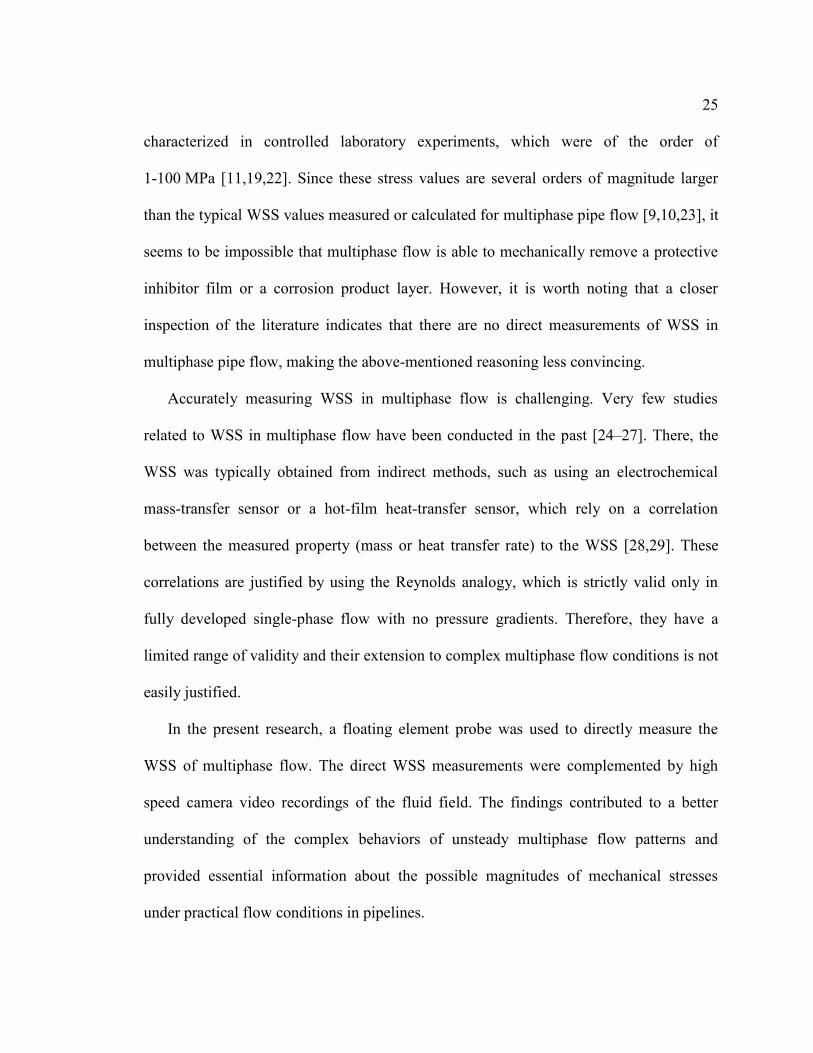
25
characterized in controlled laboratory experiments, which were of the order of
1-100 MPa [11,19,22]. Since these stress values are several orders of magnitude larger
than the typical WSS values measured or calculated for multiphase pipe flow [9,10,23], it
seems to be impossible that multiphase flow is able to mechanically remove a protective
inhibitor film or a corrosion product layer. However, it is worth noting that a closer
inspection of the literature indicates that there are no direct measurements of WSS in
multiphase pipe flow, making the above-mentioned reasoning less convincing.
Accurately measuring WSS in multiphase flow is challenging. Very few studies
related to WSS in multiphase flow have been conducted in the past [24–27]. There, the
WSS was typically obtained from indirect methods, such as using an electrochemical
mass-transfer sensor or a hot-film heat-transfer sensor, which rely on a correlation
between the measured property (mass or heat transfer rate) to the WSS [28,29]. These
correlations are justified by using the Reynolds analogy, which is strictly valid only in
fully developed single-phase flow with no pressure gradients. Therefore, they have a
limited range of validity and their extension to complex multiphase flow conditions is not
easily justified.
In the present research, a floating element probe was used to directly measure the
WSS of multiphase flow. The direct WSS measurements were complemented by high
speed camera video recordings of the fluid field. The findings contributed to a better
understanding of the complex behaviors of unsteady multiphase flow patterns and
provided essential information about the possible magnitudes of mechanical stresses
under practical flow conditions in pipelines.
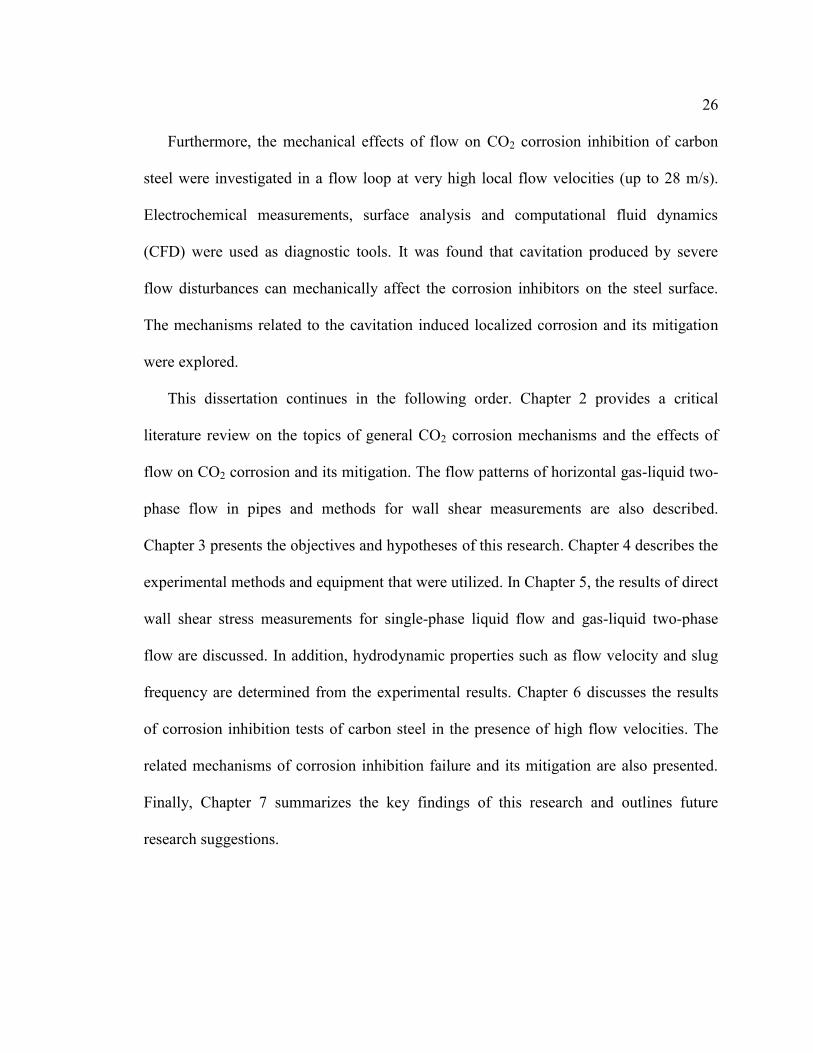
26
Furthermore, the mechanical effects of flow on CO2 corrosion inhibition of carbon
steel were investigated in a flow loop at very high local flow velocities (up to 28 m/s).
Electrochemical measurements, surface analysis and computational fluid dynamics
(CFD) were used as diagnostic tools. It was found that cavitation produced by severe
flow disturbances can mechanically affect the corrosion inhibitors on the steel surface.
The mechanisms related to the cavitation induced localized corrosion and its mitigation
were explored.
This dissertation continues in the following order. Chapter 2 provides a critical
literature review on the topics of general CO2 corrosion mechanisms and the effects of
flow on CO2 corrosion and its mitigation. The flow patterns of horizontal gas-liquid two-
phase flow in pipes and methods for wall shear measurements are also described.
Chapter 3 presents the objectives and hypotheses of this research. Chapter 4 describes the
experimental methods and equipment that were utilized. In Chapter 5, the results of direct
wall shear stress measurements for single-phase liquid flow and gas-liquid two-phase
flow are discussed. In addition, hydrodynamic properties such as flow velocity and slug
frequency are determined from the experimental results. Chapter 6 discusses the results
of corrosion inhibition tests of carbon steel in the presence of high flow velocities. The
related mechanisms of corrosion inhibition failure and its mitigation are also presented.
Finally, Chapter 7 summarizes the key findings of this research and outlines future
research suggestions.

27
Chapter 2: Background and Literature Review
2.1 Basics of CO2 Corrosion
Internal carbon dioxide (CO2) corrosion of pipeline steel is commonly seen in the oil
and gas industry. This is because carbon steel, particularly low carbon steel (generally
less than 0.30 wt.% carbon) [30], is a primary structural material for production tubing
and transportation pipelines. Carbon steel has desirable mechanical properties such as
high structural strength and low manufacturing cost. However, its corrosion resistance is
limited, and often the aqueous CO2 environment within steel pipes is corrosive.
CO2 and water are natural constituents found in petroleum reservoirs [31]. During oil
and gas production, the CO2 and water are extracted and transported together with
hydrocarbons through steel tubing and pipelines. In addition, due to global climate
change, attention has been progressively drawn to carbon capture and sequestration
(CCS) in recent decades [32–35], aiming at reducing global carbon emissions. One way
to achieve CO2 sequestration is compressing and depositing CO2 into underground
geological formations, such as depleted oil and gas wells. In the oil and gas industry, this
is frequently achieved by means of carbon dioxide enhanced oil recovery (CO2-EOR)
[36]. By injecting CO2 and/or water into mature oil fields, the CO2 is properly stored, and
the oil production is significantly increased [37]. In the above-mentioned activities, the
CO2 and water traversing tubing and pipelines create a corrosive environment and pose a
potential threat of internal corrosion [38,39]. To ensure safe operations, understanding the
CO2 corrosion mechanisms and providing means of corrosion control are of paramount
importance.

28
2.1.1 CO2 corrosion mechanisms
Mechanisms of CO2 corrosion of carbon steel have been developed over the past
decades and are considered well understood [2,3,40–43]. The process involves several
chemical and electrochemical reactions. The key chemical reactions related to CO2
corrosion are given in Table 2-1. First, gaseous CO2 dissolves in the aqueous phase
through a heterogeneous reaction (as given by Reaction (2-1)). The concentrations of
gaseous CO2 and dissolved aqueous CO2 are often of the same order of magnitude [2].
The dissolved CO2 reacts with water and forms carbonic acid (H2CO3), which is also
called the CO2 hydration reaction as given in Reaction (2-2). H2CO3, a weak acid, can
partially dissociate in water by two steps (Reactions (2-3) and (2-4)), which results in the
release of hydrogen ions (𝐻+), bicarbonate (𝐻𝐶𝑂3−) and carbonate (𝐶𝑂3
2−). In addition,
water can dissociate in an aqueous solution, releasing 𝐻+ and hydroxide ion (𝑂𝐻−).
Besides chemical reactions in the bulk, aqueous CO2 corrosion of carbon steel
involves several electrochemical reactions occurring at the steel surface. The main
anodic/oxidation reaction is the dissolution of iron, which releases ferrous ions (𝐹𝑒2+)
into the solution leaving behind the electrons (𝑒−). Multiple cathodic/reduction reactions
occur in the CO2 corrosion process. The released electrons from iron are taken up by the
readily available chemical species at the surface through reduction reactions, which are
also called hydrogen evolution reactions as dissolved hydrogen gas is the common
reaction product. The main electrochemical reactions of CO2 corrosion are given in Table
2-2.

29
Table 2-1: Key chemical reactions of aqueous CO2 corrosion and the corresponding
chemical equilibrium expressions
Reaction Chemical equilibrium expression
𝐶𝑂2 (𝑔)
𝐾𝑠𝑜𝑙
⇌ 𝐶𝑂2 (𝑎𝑞) 𝐾𝑠𝑜𝑙 =𝑐𝐶𝑂2
𝑝𝐶𝑂2
(2-1)
𝐶𝑂2 (𝑎𝑞) + 𝐻2𝑂(𝑙)
𝐾ℎ𝑦
⇌ 𝐻2𝐶𝑂3 (𝑎𝑞) 𝐾ℎ𝑦 =𝑐𝐻2𝐶𝑂3
𝑐𝐶𝑂2
(2-2)
𝐻2𝐶𝑂3 (𝑎𝑞)
𝐾𝑐𝑎
⇌ 𝐻+(𝑎𝑞) + 𝐻𝐶𝑂3
−(𝑎𝑞)
𝐾𝑐𝑎 =𝑐𝐻+𝑐𝐻𝐶𝑂3
−
𝑐𝐻2𝐶𝑂3
(2-3)
𝐻𝐶𝑂3−
(𝑎𝑞)
𝐾𝑏𝑖
⇌ 𝐻+(𝑎𝑞) + 𝐶𝑂3
2−(𝑎𝑞)
𝐾𝑏𝑖 =𝑐𝐻+𝑐𝐶𝑂3
2−
𝑐𝐻𝐶𝑂3−
(2-4)
𝐻2𝑂(𝑙)
𝐾𝑤𝑎
⇌ 𝐻+(𝑎𝑞) + 𝑂𝐻−
(𝑎𝑞) 𝐾𝑤𝑎 = 𝑐𝐻+𝑐𝑂𝐻− (2-5)
Table 2-2: Key electrochemical reactions of aqueous CO2 corrosion
Anodic 𝐹𝑒 (𝑠) 𝐹𝑒2+(𝑎𝑞) + 2𝑒− (2-6)
Cathodic 2𝐻+(𝑎𝑞) + 2𝑒− 𝐻2 (𝑔) (2-7)
Cathodic 2𝐻2𝐶𝑂3 (𝑎𝑞) + 2𝑒− 𝐻2 (𝑔) + 2𝐻𝐶𝑂3−
(𝑎𝑞) (2-8)
Cathodic 2𝐻𝐶𝑂3−
(𝑎𝑞)+2𝑒− 𝐻2 (𝑔) +2𝐶𝑂3
2−(𝑎𝑞)
(2-9)
Cathodic 2𝐻2𝑂(𝑙) +2𝑒− 𝐻2 (𝑔) +2𝑂𝐻−(𝑎𝑞) (2-10)
30
From Table 2-1 and Table 2-2, the overall reaction of CO2 corrosion of carbon steel
may be summarized by the following reaction:
𝐹𝑒 (𝑠) + 𝐶𝑂2 (𝑎𝑞) + 𝐻2𝑂(𝑙) ⇌ 𝐹𝑒2+(𝑎𝑞) + 𝐶𝑂3
2−(𝑎𝑞) + 𝐻2(𝑔) (2-11)
It can be seen that ferrous ion and carbonate ion are products of CO2 corrosion. If the
concentrations of these two species in the solution are sufficiently high, precipitation of
solid iron carbonate (FeCO3) will occur, as shown by:
𝐹𝑒2+(𝑎𝑞) + 𝐶𝑂3
2−(𝑎𝑞)
𝐾𝑠𝑝
⇋ 𝐹𝑒𝐶𝑂3 (𝑠) (2-12)
Due to the reversible nature of this reaction, the solid iron carbonate can also dissolve in
the solution when the ferrous ion and carbonate ion concentrations are below the
saturation level.
2.1.2 Mitigation of CO2 corrosion
In the previous section, the main reactions in aqueous CO2 corrosion of carbon steel
are concisely presented. In this section, the common approaches to mitigate CO2
corrosion are introduced.
2.1.2.1 Formation of a protective FeCO3 corrosion product layer
As described earlier, a FeCO3 layer can form in CO2 corrosion as long as the
concentrations of ferrous and carbonate ions are above saturation. The saturation criterion
of FeCO3 layer formation is quantitatively defined as supersaturation, 𝑆(𝐹𝑒𝐶𝑂3), given by:
31
𝑆(𝐹𝑒𝐶𝑂3) =𝑐𝐹𝑒2+𝑐𝐶𝑂3
2−
𝐾𝑠𝑝 (2-13)
where 𝑐𝐹𝑒2+ and 𝑐𝐶𝑂32− are the concentrations of ferrous ion and carbonate ion,
respectively, and 𝐾𝑠𝑝 is the solubility product constant of FeCO3. This equation
represents the balanced reactions of FeCO3 precipitation and dissolution. When 𝑆(𝐹𝑒𝐶𝑂3)
is greater than 1, the precipitation reaction prevails and a FeCO3 layer may form on the
steel surface. Conversely, no FeCO3 layer is expected when the 𝑆(𝐹𝑒𝐶𝑂3) is less than 1, as
the dissolution process is dominant. The 𝑆(𝐹𝑒𝐶𝑂3) is greatly dependent on the pH and
𝑐𝐹𝑒2+ . When substituting the equilibrium expressions presented in Table 2-1 into
Reaction (2-13), the saturation value can be written as:
𝑆(𝐹𝑒𝐶𝑂3) =𝑐𝐹𝑒2+𝐾𝑏𝑖𝐾𝑐𝑎𝐾ℎ𝑦𝐾𝑠𝑜𝑙𝑝𝐶𝑂2
𝐾𝑠𝑝𝑐𝐻+ (2-14)
where 𝑝𝐶𝑂2 is the partial pressure of CO2 in the gas phase. The reaction constants are
functions of temperature, pressure and ionic strength [2].
The characteristics of the FeCO3 layer have been studied by various researchers
[5,7,44]. It is generally accepted that a complete coverage of FeCO3 on a steel surface
leads to protection because this layer presents a mass transfer barrier for corrosive species
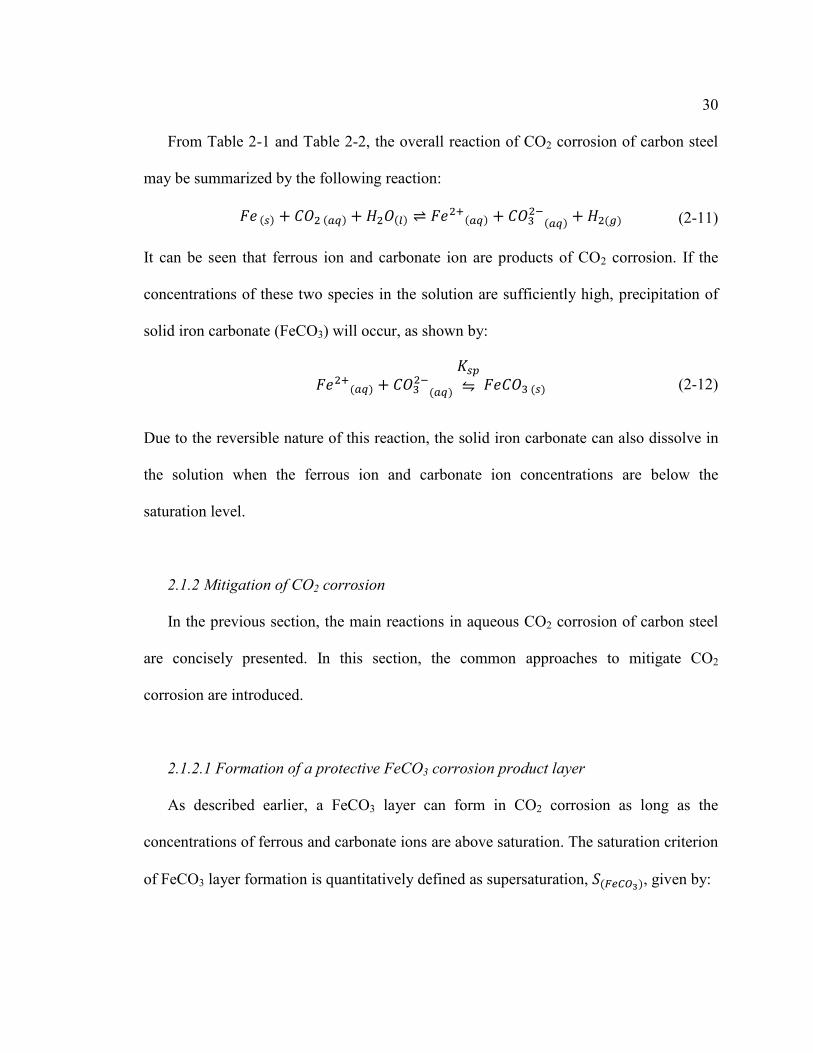
and slows down the corrosion process. To illustrate this by an example, Figure 2-1 shows
the topography of a steel surface entirely covered by a dense FeCO3 layer consisting of
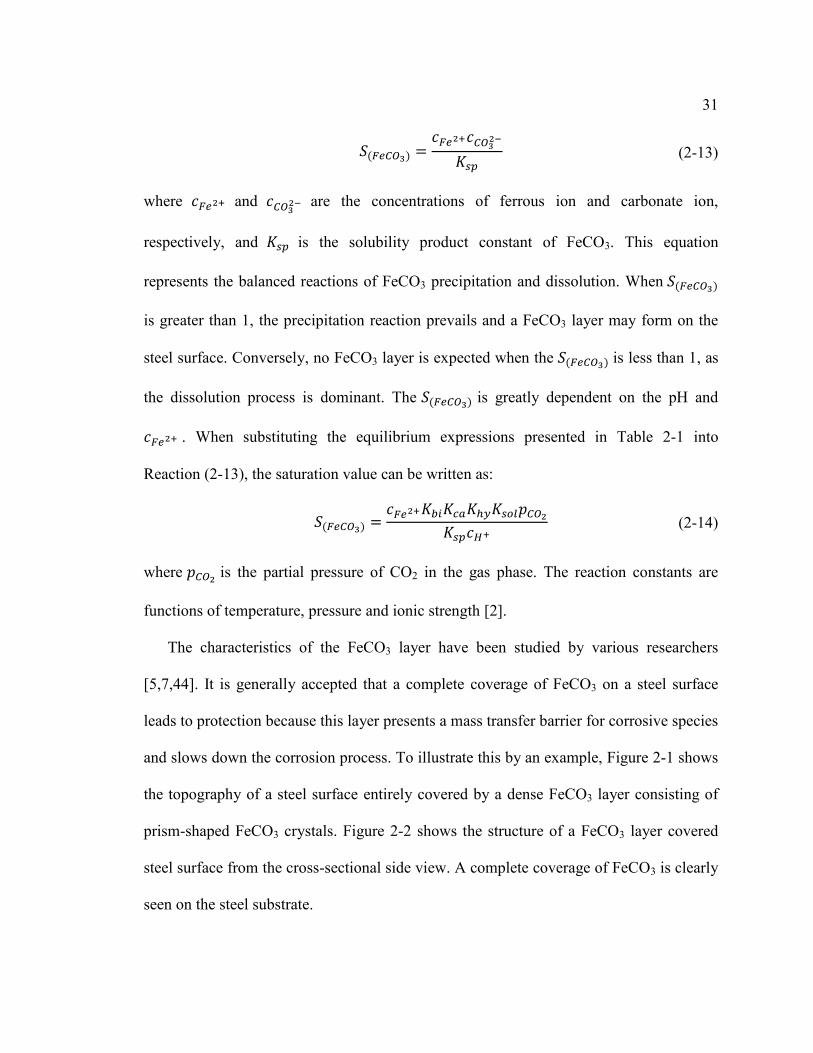
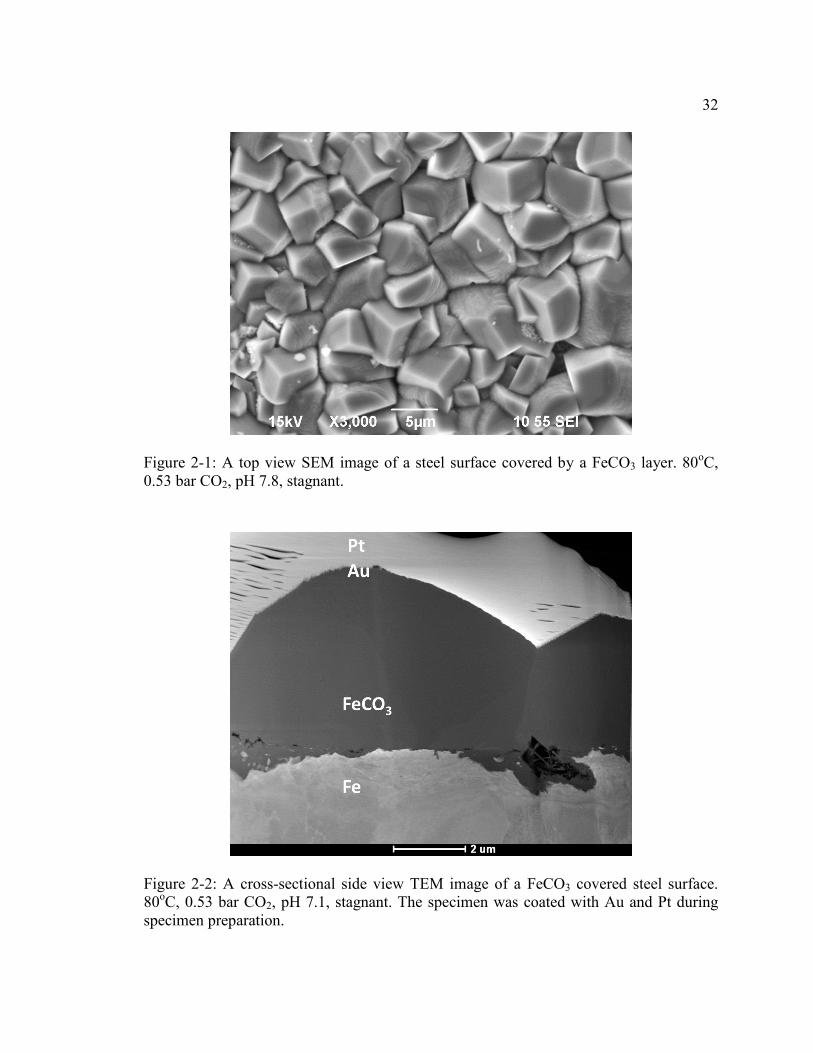
prism-shaped FeCO3 crystals. Figure 2-2 shows the structure of a FeCO3 layer covered
steel surface from the cross-sectional side view. A complete coverage of FeCO3 is clearly
seen on the steel substrate.
32
Figure 2-1: A top view SEM image of a steel surface covered by a FeCO3 layer. 80oC, 0.53 bar CO2, pH 7.8, stagnant.
Figure 2-2: A cross-sectional side view TEM image of a FeCO3 covered steel surface. 80oC, 0.53 bar CO2, pH 7.1, stagnant. The specimen was coated with Au and Pt during specimen preparation.
33
Multiple researchers [6,8,45] found that the corrosion rate was significantly retarded
when the steel surface was fully covered by a FeCO3 layer; this decrease of corrosion rate
was accompanied by a dramatic increase of open circuit potential. This behavior was
termed pseudo-passivation [8] as the FeCO3 layer offered a corrosion protection similar
to metal passivation in the sense that the corrosion potential becomes more positive as the
corrosion rate is reduced. Pseudo-passivation was usually observed at a relatively high
pH, which favored the precipitation of FeCO3. The dependence of FeCO3 precipitation on
pH is revealed by Equation (2-14). In laboratory experiments Han et al. [8] observed the
pseudo-passivation at a pH of 8.0 and identified a trace amount of Fe3O4 within the
FeCO3 layer. Li et al. [6] found that pseudo-passivation occurred with a pH higher than
6.0 at 80oC and 0.53 bar CO2.
Generally, FeCO3 forms a protective corrosion product layer against internal
corrosion of pipelines when the environment has a high pH value. For example, de
Moraes et al. found that a very protective FeCO3 layer formed in a flow loop at a pH
higher than 5.5 at 93oC [46]. Therefore, formation of protective FeCO3 layers under
specific conditions is deemed an effective means to mitigate CO2 corrosion.
2.1.2.2 CO2 Corrosion inhibitors
It was stated above that FeCO3 corrosion product layers can provide corrosion
protection for systems with a relatively high pH value. For systems with more acidic
conditions, other corrosion mitigation approaches are required since no protective FeCO3
corrosion product layer would form on the steel surface. In the oil and gas industry,

34
applications of corrosion inhibitors are often deemed a cost-effective alternative to
mitigate internal corrosion [39].
In general, corrosion inhibitors are chemical compounds added to aqueous
environments in small concentrations which interact with the metal surface and reduce
the oxidation rate of the metal [47]. The chemical corrosion inhibition process comprises
two steps, mass transport of inhibitors from the bulk to the steel surface and interactions
between the inhibitors and the steel surface [47]. Corrosion inhibitors have been
generally classified as three types [48]: Type A inhibitors adsorb on the steel surface to
form a protective inhibitor film that prevents corrosive species reaching the steel surface;
Type B inhibitors change the solution chemistry and reduce the corrosivity of the
environment, e.g., oxygen scavengers; and Type C inhibitors possess the properties of
both Type A and Type B inhibitors.
An extensive amount of corrosion inhibitors fall into Type A, which are usually
organic compounds [4,47–49]. These organic compounds are typically surface-active
agents, or surfactants, which are amphiphilic. This is because a surfactant molecule
contains both hydrophobic (non-polar tail) and hydrophilic (polar head) groups. The
hydrophobic tails are long hydrocarbon chains (usually C6 to C22 [50]), while the
hydrophilic heads are either non-ionic or ionic functional groups. Surfactants with ionic
hydrophilic heads can be further classified as anionic, cationic and zwitterionic types
[51], depending on the electrical charge on the heads. Anionic type surfactants have
negative charge on the head groups; cationic type surfactants have head groups carrying

35
positive charge. For zwitterionic type surfactants, the heads contain both positively and
negatively charged groups [52].
Due to their amphiphilic nature, surfactant inhibitors tend to adsorb orderly at
interfaces [51]. Therefore, surfactants provide corrosion protection by forming an
adsorbed film at the metal-solution interface. Adsorption of surfactants depends on a
variety of factors, such as the nature of the substrate (adsorbent), the chemical and
structural properties of the surfactant molecule (adsorbate), and the environment (e.g.,
temperature, pH and electrolyte) [51]. Generally, adsorption of surfactants is attributed to
intermolecular interactions, which include electrostatic interactions, hydrophobic
interactions, covalent bonding and hydrogen bonding [53].
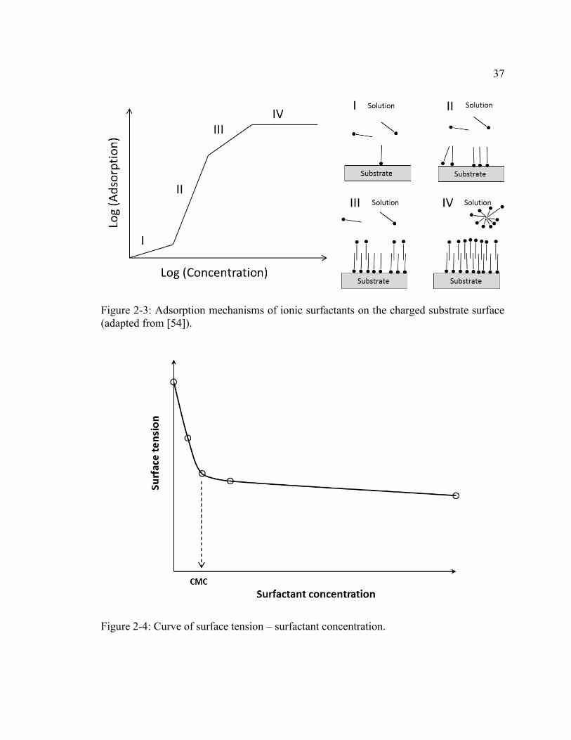
The adsorption of ionic surfactants is mainly driven by electrostatic and hydrophobic
interactions [54]. The mechanisms of ionic surfactant adsorption on oppositely charged
surfaces have been extensively studied by using adsorption isotherms and are reasonably
well understood [53–55]. The adsorption isotherm of ionic surfactants is typically
classified by four regions [53,54], as shown in Figure 2-3. In region I, the surfactant
concentration is low and the dominating driving force for adsorption is the electrostatic
interaction between the hydrophilic head group of individual surfactant molecules and the
charged substrate surface. The adsorbed surfactants on the surface are present in the form
of single molecules unassociated with each other [53]. In region II, besides the
electrostatic interactions, the hydrophobic interactions between the hydrophobic tail
groups of the adsorbed molecules become significant, which lead to the formation of a
monolayer by aggregation. Due to this additional driving force, the adsorption in this

36
region is drastically increased. At the end of this region, the surface is electrically
neutralized by the oppositely charged surfactant ions [53,54]. In region III, as
electrostatic interactions in direct association with the surface are no longer possible,
increase of adsorption with a reduced rate occurs due to the hydrophobic interactions
between the non-polar tails of the adsorbed surfactants and the free surfactants in the bulk,
which results in the structural growth of the aggregates; in the figure this is shown as
bilayer formation. In region IV, when further adding surfactants to the system above a
threshold concentration, the steel surface is saturated with aggregates and reaches
maximum coverage, and the excess surfactants form micelles in the bulk solution. Due to
the hydrophobicity, the micelles have structures in which the hydrophobic groups of the
molecules stick together and the hydrophilic groups face toward the aqueous environment.
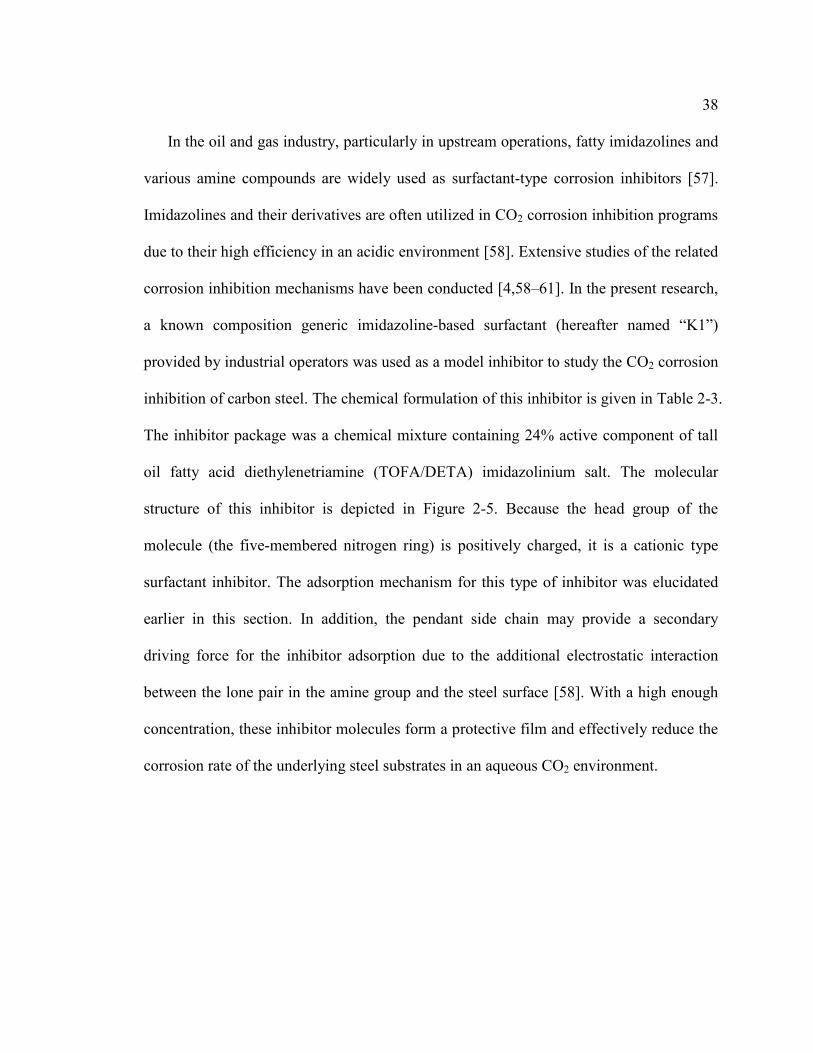
This threshold concentration is referred to as the critical micelle concentration (CMC). It
is defined as the minimum concentration of surfactants at which micelles can be detected
and all additional surfactants form micelles [56]. The CMC features abrupt changes in the
physical properties of the solution such as surface or interfacial tension, electrical
conductivity, and light scattering [51]; these characteristics are practically used for the
determination of the CMC value. For example, Figure 2-4 shows a surface tension-
concentration curve, where a sharp change of surface tension around CMC can be seen.
37
Figure 2-3: Adsorption mechanisms of ionic surfactants on the charged substrate surface (adapted from [54]).
Figure 2-4: Curve of surface tension – surfactant concentration.
38
In the oil and gas industry, particularly in upstream operations, fatty imidazolines and
various amine compounds are widely used as surfactant-type corrosion inhibitors [57].
Imidazolines and their derivatives are often utilized in CO2 corrosion inhibition programs
due to their high efficiency in an acidic environment [58]. Extensive studies of the related
corrosion inhibition mechanisms have been conducted [4,58–61]. In the present research,
a known composition generic imidazoline-based surfactant (hereafter named “K1”)
provided by industrial operators was used as a model inhibitor to study the CO2 corrosion
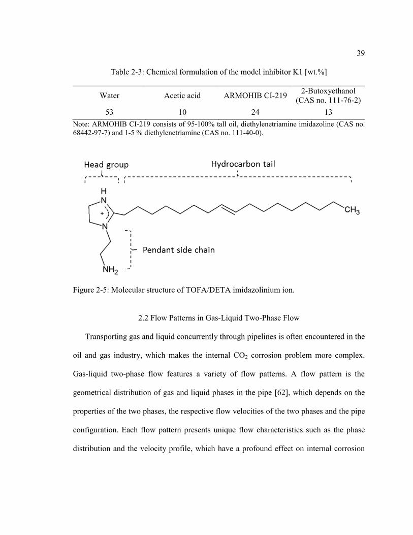
inhibition of carbon steel. The chemical formulation of this inhibitor is given in Table 2-3.
The inhibitor package was a chemical mixture containing 24% active component of tall
oil fatty acid diethylenetriamine (TOFA/DETA) imidazolinium salt. The molecular
structure of this inhibitor is depicted in Figure 2-5. Because the head group of the
molecule (the five-membered nitrogen ring) is positively charged, it is a cationic type
surfactant inhibitor. The adsorption mechanism for this type of inhibitor was elucidated
earlier in this section. In addition, the pendant side chain may provide a secondary
driving force for the inhibitor adsorption due to the additional electrostatic interaction
between the lone pair in the amine group and the steel surface [58]. With a high enough
concentration, these inhibitor molecules form a protective film and effectively reduce the
corrosion rate of the underlying steel substrates in an aqueous CO2 environment.
39
Table 2-3: Chemical formulation of the model inhibitor K1 [wt.%]
Water Acetic acid ARMOHIB CI-219 2-Butoxyethanol (CAS no. 111-76-2)
53 10 24 13 Note: ARMOHIB CI-219 consists of 95-100% tall oil, diethylenetriamine imidazoline (CAS no. 68442-97-7) and 1-5 % diethylenetriamine (CAS no. 111-40-0).
Figure 2-5: Molecular structure of TOFA/DETA imidazolinium ion.
2.2 Flow Patterns in Gas-Liquid Two-Phase Flow
Transporting gas and liquid concurrently through pipelines is often encountered in the
oil and gas industry, which makes the internal CO2 corrosion problem more complex.
Gas-liquid two-phase flow features a variety of flow patterns. A flow pattern is the
geometrical distribution of gas and liquid phases in the pipe [62], which depends on the
properties of the two phases, the respective flow velocities of the two phases and the pipe
configuration. Each flow pattern presents unique flow characteristics such as the phase
distribution and the velocity profile, which have a profound effect on internal corrosion
40
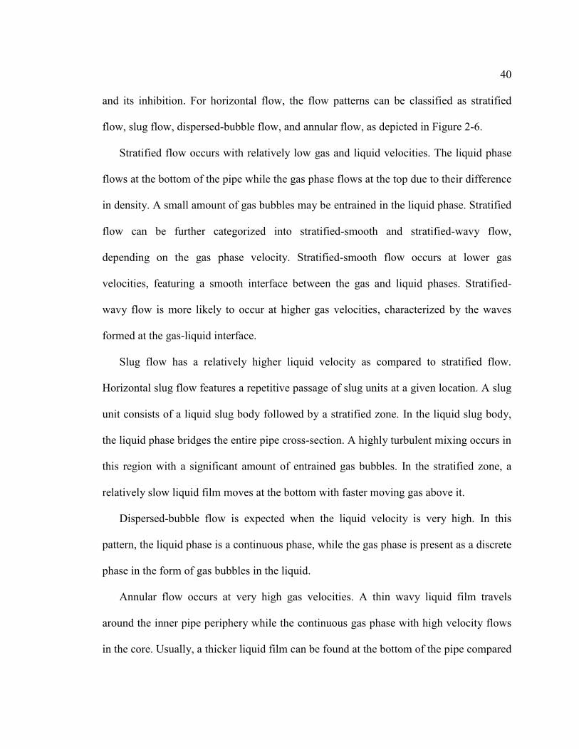
and its inhibition. For horizontal flow, the flow patterns can be classified as stratified
flow, slug flow, dispersed-bubble flow, and annular flow, as depicted in Figure 2-6.
Stratified flow occurs with relatively low gas and liquid velocities. The liquid phase
flows at the bottom of the pipe while the gas phase flows at the top due to their difference
in density. A small amount of gas bubbles may be entrained in the liquid phase. Stratified
flow can be further categorized into stratified-smooth and stratified-wavy flow,
depending on the gas phase velocity. Stratified-smooth flow occurs at lower gas
velocities, featuring a smooth interface between the gas and liquid phases. Stratified-
wavy flow is more likely to occur at higher gas velocities, characterized by the waves
formed at the gas-liquid interface.
Slug flow has a relatively higher liquid velocity as compared to stratified flow.
Horizontal slug flow features a repetitive passage of slug units at a given location. A slug
unit consists of a liquid slug body followed by a stratified zone. In the liquid slug body,
the liquid phase bridges the entire pipe cross-section. A highly turbulent mixing occurs in
this region with a significant amount of entrained gas bubbles. In the stratified zone, a
relatively slow liquid film moves at the bottom with faster moving gas above it.
Dispersed-bubble flow is expected when the liquid velocity is very high. In this
pattern, the liquid phase is a continuous phase, while the gas phase is present as a discrete
phase in the form of gas bubbles in the liquid.
Annular flow occurs at very high gas velocities. A thin wavy liquid film travels
around the inner pipe periphery while the continuous gas phase with high velocity flows
in the core. Usually, a thicker liquid film can be found at the bottom of the pipe compared
41
to that at the top [62]. In addition, part of the liquid will be entrained and travel as
discrete droplets in the gas core. Due to the presence of entrained liquid droplets, this
flow pattern is also called annular-dispersed flow.
Figure 2-6: Schematics of flow patterns in horizontal gas-liquid two-phase flow (adapted from [62]).
As described, the flow patterns are strongly dependent on the flow velocities of the
gas and liquid phases. Transitions between flow patterns can be represented by a flow
pattern map constructed with respect to the gas and liquid flow velocities, as illustrated in
Figure 2-7. For two-phase flow, the superficial velocities are usually used, which are
defined as the volumetric flow rate of the phase divided by the cross-sectional area of the
full pipe.
42
So far, the main flow patterns of gas-liquid two-phase flow have been described.
Compared to single-phase flow, two-phase flow usually features inhomogeneous phase
distributions and is highly turbulent. Therefore, the effect of two-phase flow on CO2
corrosion is deemed more complex.
Figure 2-7: A flow pattern map for horizontal gas-liquid two-phase flow. H2O / CO2, 25oC, 1 bar, 4 inch ID pipe (generated by an in-house gas-liquid flow model [63]).
2.3 Effects of Flow on Mitigation of CO2 Corrosion
It was mentioned earlier that a complete coverage of protective FeCO3 layers or
corrosion inhibitor films on the steel surface can significantly reduce the corrosion rate.
However, any partial damage or removal of these films or layers may lead to severe
localized corrosion [8,9]. In this section, several effects of flow on the integrity of
protective inhibitor films and corrosion product layers are discussed.
43
2.3.1 Effect of mass transfer
Flow enhances the mass transport of corrosive species from bulk solution to the steel
surface and accelerates the corrosion of the underlying steel [2]. In CO2 corrosion,
because all the electrochemical reactions simultaneously occur at the metal-solution
interface, the mass transport of reactants (e.g., H+) from bulk to the metal surface is
usually involved. If the mass transport cannot provide enough reactants to the steel
surface where the fast electrochemical reactions occur, the corrosion rate/current will be
affected by the mass transport process, referred to as mass transfer limiting current [64].
The mass transfer effect of flow on electrochemical reactions occurring at the metal
surface can be best illustrated by using the oxidation-reduction reactions of the
ferricyanide-ferrocyanide couple [65], which are written as:
[𝐹𝑒(𝐶𝑁)6]3−(𝑎𝑞)
+ 𝑒− ⇌ [𝐹𝑒(𝐶𝑁)6]4−(𝑎𝑞)
(2-15)
For example, Figure 2-8 shows the measured mass transfer limiting currents for the
anodic and cathodic reactions of the ferri/ferrocyanide couple on a nickel rotating
cylinder electrode (RCE) in an alkaline solution (See Appendix 1 for more details). It
clearly demonstrates that the mass transfer limiting currents increase with an increasing
flow velocity. The flow dependent electrochemical limiting current is often measured to
calculate the mass transfer coefficient (𝑘𝑚) with the following formula [65]:
𝑘𝑚 =𝑖𝑙𝑖𝑚
𝑛𝑒𝐹𝐴𝐶𝑏 (2-16)
where 𝑖𝑙𝑖𝑚 is the mass transfer limiting current; 𝑛𝑒 is the number of electrons in the
reaction; 𝐹 is the Faraday’s constant; 𝐴 is the surface area of the electrode; and 𝐶𝑏 is the
bulk concentration of the reactant.

44
Figure 2-8: Potentiodynamic polarization curves measuring the mass transfer limiting currents of the ferri/ferrocyanide. Nickel RCE electrode (a diameter of 12 mm and length of 14 mm), 25oC, 2 M NaOH, 0.01 M K4[Fe(CN)6] / K3[Fe(CN)6], 1 bar N2.
Flow may not only enhance the mass transport of corrosive species toward the steel
surface, but also interfere with the FeCO3 layer formation by facilitating the mass
transport of the corrosion-generated ferrous ions (Fe2+) away from the steel surface. In
acidic conditions such as CO2 corrosion, a decrease of Fe2+ concentration and increase of
H+ concentration at the surface by enhanced mass transport result in a lower saturation
value for FeCO3 according to Equation (2-14), which hinders the formation of protective
FeCO3 layers.
45
2.3.2 Effect of mechanical forces
The effect of mechanical forces exerted by flow on the integrity of inhibitor films or
FeCO3 layers is not well understood. Prevalent thinking is that high magnitude stresses
produced by turbulent flow (e.g., WSS) mechanically damage the protective films or
layers, resulting in partial removal of these films or layers from the steel surface and
leading to accelerated corrosion rates or even severe localized corrosion [9,13]. This
postulate seems to be supported by some field experience and laboratory observations.
For example, Pots et al. executed a series of field tests and found that the corrosion
inhibitor failed above certain flow velocities [14]. They assumed that the high WSS was
the cause for the corrosion inhibitor failure. In another laboratory study Ruzic et al.
observed the mechanical removal of FeCO3 layers on a rotating cylinder electrode at high
rotating speeds. It was suspected that severe local WSS fluctuations exceeding the
adhesive strength of the layers resulted in a fatigue-type damage [12]. Upon careful
examination of the results, it is found that occurrence of high WSS is often inevitably
coupled with other possible influencing factors in the high flow velocity environments,
such as enhanced mass transfer rate and changed local water chemistry, formation of
bubbles and droplets in multiphase flow, etc. Therefore, one could not always conclude
that it is the WSS that causes to the failures of these protective films or layers, as was
often done in the past, but rather only that WSS correlates with failures of these
protective films or layers. Correlation does not always mean causation.
In other detailed laboratory experiments focused on the pure mechanical effect of
flow, no failure of these films or layers due to WSS was found. Gulbrandsen and Grana
46
[17] used a jet impingement setup and found that the CO2 corrosion inhibitor
performance was independent of flow velocity up to 20 m/s with a calculated WSS up to
1400 Pa. They also observed that ingress of O2 in the flow system greatly accelerated the
corrosion rate due to the enhanced mass transfer rate of O2 by the highly turbulent flow.
In a very different flow geometry in a thin channel, Farelas found that the flow with a
WSS value up to 350 Pa (flow velocity up to 13.8 m/s) was unable to mechanically
remove the formed FeCO3 layer on the steel surface [18].
With the inconsistency in the existing literature, the question as to whether flow could
mechanically damage the protective inhibitor films and corrosion product layers remains
unanswered. Obtaining the answer requires accurate measurements of the adhesion
strength of these films / layers to the steel surface and the magnitudes of WSS exerted by
flow. The adhesion strength of these films and layers has been previously characterized in
controlled laboratory experiments. For example, the adhesion strength of the FeCO3 layer
to a steel substrate was measured by tensile testing [11,19]. In these experiments, an
external stud was glued to a FeCO3 layer pre-formed on the steel surface by using a
strong adhesive and then separated. The required separation force was measured, and the
adhesion strength of the FeCO3 layers to the steel surface was calculated to be of the
order of 1 - 10 MPa. In another study, Xiong et al. [22] used atomic force microscopy
(AFM) to mechanically remove an inhibitor film from a steel surface. The adsorbed
inhibitor film was “scratched” away by the lateral movements of the AFM tip that was in
contact with the steel surface. The required lateral forces to remove the inhibitor
molecules from the steel surface were calculated to be of the order of 50 - 100 MPa. The
47
experimental findings suggest that the adhesion strength of these protective films or
layers is of the order of MPa. On the other hand, typical WSS values measured or
calculated in multiphase pipe flow are of the order of 1 Pa–1 kPa [9,10,23]. Some
researchers focused on the local fluctuations of turbulence by analyzing the
electrochemical current noise data, they claimed that flow could generate a MPa
magnitude turbulent energy density [9,66]. However, their conclusions were based only
on indirect correlations and mathematic manipulations of the mass transfer
electrochemical current noise data. No direct experimental evidence or the Direct
Numerical Simulation (DNS) 1 data obtained in single phase liquid flow, indicates that
flow can generate a WSS of such magnitude.
Since the adhesion strength values of the inhibitor films or corrosion product layers
are several orders of magnitude larger than the generally believed WSS values in
practical pipe flow systems, doubts exist as to whether multiphase flow is able to
mechanically remove a protective film or corrosion product layer. However, a closer
inspection of literature sources indicates that there are no direct measurements for WSS
in multiphase pipe flow. Therefore, accurate measurements of the WSS for multiphase
flow become imperative to answer the above-mentioned questions. The current available
techniques for WSS measurements are reviewed in the following section.
1 DNS is a numerical technique where the Navier Stokes equations are solved fully in time and space resulting in an unrestricted access to all the key aspects of the flow field.
48
2.3.3 Other miscellaneous effects found in multiphase flow
Other miscellaneous effects found in multiphase flow complicate the problem of CO2
corrosion mitigation, such as condensation in so called Top-of-the-line corrosion (TLC)
and the presence of solids in the flow [10].
TLC corrosion occurs in “wet” gas transportation pipelines with a stratified flow
pattern due to the water condensation at the top of the internal pipe wall, where the
saturated vapor inside the pipe is cooled by the surrounding environment being at a much
lower temperature [10]. The condensed water at the steel surface contains dissolved gases
such as CO2, which locally forms a corrosive environment and leads to severe localized
corrosion problems [67]. Due to the stratified flow pattern, mitigation of TLC by
injection of corrosion inhibitors is challenging because the inhibitors in the liquid phase
flowing at the bottom of the pipe may not reach the top of the pipe [10].
The presence of solids in pipe flow is often problematic. At low flow rates, solid
particles precipitate at the bottom of the pipe and drastically change the local flow and
water chemistry, leading to so called under-deposit corrosion. The solids may also
influence the corrosion inhibition process. It was found that sand particles can adversely
affect the inhibitor adsorption in the crevices between the settled particles and the
underlying steel surface, resulting in severe localized corrosion due to the formation of
galvanic cells [20]. At high flow rates, entrained solid particles in the flow stream
frequently impinge on the pipe wall. The particle-wall impacts may cause damage to the
protective corrosion product layers or prevent the formation of such layers [21], which is
often termed erosion-corrosion.
49
2.4 Wall Shear Stress Measurements
Answering the question as to whether flow is able to mechanically remove protective
corrosion product layers and inhibitor films relies on accurate measurements of WSS.
Numerous methods for WSS determination have been developed in the past decades,
which may be grouped as shown in Figure 2-9. Several prevalent methods of WSS
measurements in flow studies are outlined below.
Figure 2-9: Classification of methods for wall shear stress measurements (adapted from [68–70]).
2.4.1 Direct measurements
Direct measurements of WSS are achieved by using a mechanical device with an
element flush mounted on the wall that allows for lateral movements, often termed a
floating element (as shown in Figure 2-10). The force exerted by the flow shear on the
floating element results in displacement of the floating element, which is a function of the
mechanical properties of the device. The displacement is directly correlated to the exerted
50
mechanical force on the floating element, by which the WSS is determined. The main
advantage of this method is that the WSS is directly measured and no other assumptions
are necessary. The historical prototypes of this device did have some shortcomings.
Winter et al. [68] listed the experimental deficiencies as the effects of misalignment of
the element, temperature changes, the necessary gaps around the floating element, heat
transfer, etc.
Figure 2-10: Schematic of classical floating element WSS sensor (adapted from [69]).
In order to address these issues, several modifications of this device have been
recently implemented. The microelectromechanical systems (MEMS) based floating
element sensors have been progressively developed for WSS measurement [28,69,71].
Thanks to the development of micromachining, this miniature floating element, usually
with dimensions of the order of 1-1000 µm [69], successfully solves problems related to
its conventional macroscale counterparts such as the influence of gaps and misalignment
of the element [28].
In principle, direct measurements rely on accurately measuring the lateral
displacement of the floating element. The displacement can be measured by using

51
transduction techniques such as piezoresistive or capacitive detection [69]. Piezoresistive-
type and capacitive-type floating elements change their electrical resistivity and
capacitance, respectively, when they are under mechanical strain. These techniques have
good sensitivity for mechanical stress. However, a major drawback is that they are also
very sensitive to temperature and electromagnetic interference. In addition, it is not easy
to isolate WSS from normal pressure forces exerted on the floating element. The optical
technique is also used to accurately detect the lateral displacement of the floating element
[69]. In one design of an optical-based WSS sensor [72], two photodiodes are mounted
underneath the floating element, measuring the light from a laser source above the
floating element. The displacement of the floating element due to WSS results in partial
blockage of the light to the photodiodes. The change of the current signals transmitted by
the photodiodes is directly related to the WSS exerted on the floating element. This
technique requires an optically clean working environment, which is not easy to satisfy in
liquid turbulent pipe flow.
The MEMS-based floating element significantly improves both the temporal and
spatial resolution of the measurements due to its small physical dimensions and reduced
inertia [28]. This type of device is often used in turbulent gas flow, especially in the
aerospace industry, where accurate measurements of small WSS fluctuations are
demanded [69]. This modified device has also been used in liquid environments, although
infrequently. Shajii et al. [73] fabricated a floating element sensor with a surface
dimension of 120 µm × 140 µm and tested its performance in liquid flow generated by a
viscometer. It was claimed to have a measurement range from 1–100 kPa. However, due
52
to the low sensitivity, it was not readily applicable to liquid turbulent flow [69]. From this
brief review, it appears that most of the earlier floating element WSS sensors are not
robust enough for working in turbulent single-phase and multiphase flow that is similar to
field conditions seen in the oil and gas industry.
Recently, another noticeable modification to the floating element sensor has been
made by Lenterra, Inc. [74]. In their WSS probe design, the displacement of the floating
element is measured using optical strain gauges. The floating element is connected to a
mechanical cantilever. Two optical fiber strain gauges, with fiber Bragg grating (FBG),
are attached to the cantilever. The top face of the floating element flush mounted on the
internal pipe wall is laterally displaced when there is fluid shearing over its surface. Any
movement of the floating element causes bending (mechanical deformation) of the
cantilever, which changes the optical reflection spectra obtained from the attached strain
gauges. The optical spectra are then processed followed by straightforward mechanical
calculations that indicate the WSS value. Using two optical fiber strain gauges solves the
problem of influence of temperature and has a measurement range (0.1 Pa to 1 kPa) close
to the WSS values expected in practical liquid flow conditions. Due to the usage of
durable fabrication materials such as stainless steel and glass fibers in this sensor, it is
robust for WSS measurements in a liquid turbulent flow environment. Therefore, this
floating element sensor was used in the present experimental study; the details will be
introduced later.
53
2.4.2 Indirect measurements
Sensors using indirect methods are often employed for WSS measurements,
especially in liquid turbulent flow, because they are generally easier to manufacture and
more robust than floating element sensors [28]. All indirect methods rely on a theoretical
or empirical correlation between the measured properties to the WSS through a set of
assumptions. Several indirect methods, with their advantages and disadvantages, are
given below.
2.4.2.1 Pressure-difference based methods
Pressure-difference based methods, such as the Preston tube and the Stanton tube, are
relatively simple to use for estimating the average shear stress. There is generally no
direct correlation between WSS and pressure difference except in fully developed
horizontal pipe flow [70], where the time-averaged WSS (𝜏̅) can be calculated from the
streamwise pressure drop over a certain pipe length, as given by:
𝜏̅ =𝐷
4(−
𝑑𝑃
𝑑𝑥) (2-17)
where D is the pipe diameter. This relationship is therefore often used for the calibration
of other pressure-difference based WSS measurement methods.
The Preston tube and the Stanton tube are actually Pitot tubes resting on the pipe wall
for pressure measurements, from which the flow velocities are determined. The measured
velocities (�̅�) are correlated with the WSS by using the law of the wall of the viscous
sublayer, as given by [29]:
54
�̅� =𝜏̅
µ𝑦 (2-18)
where µ is the dynamic viscosity of the fluid and 𝑦 is the distance to the wall. By
calibrating with fully developed pipe flow (Equation (2-17)), the pressure measurements
from the Preston tube and the Stanton tube can be related to WSS values [29].
The Preston tube and Stanton tube require a near-wall flow model (e.g., the law of the
wall) and knowledge of the fluid properties (e.g., viscosity). In addition, physical
obstacles in the pipes may interfere with the flow field [29], negatively affecting the
accuracy of measurements. Last, but not least, these methods do not offer a temporal
resolution for measuring the fluctuations in the flow.
2.4.2.2 Methods based on Reynolds analogy
The hot-film heat transfer sensor and the electrochemical mass transfer sensor have
enjoyed popularity for WSS measurements [10,24,28,29]. Both methods rely on the
Reynolds analogy between momentum transfer and heat/mass transfer. The principle of
heat transfer and mass transfer WSS sensors is illustrated in Figure 2-11.
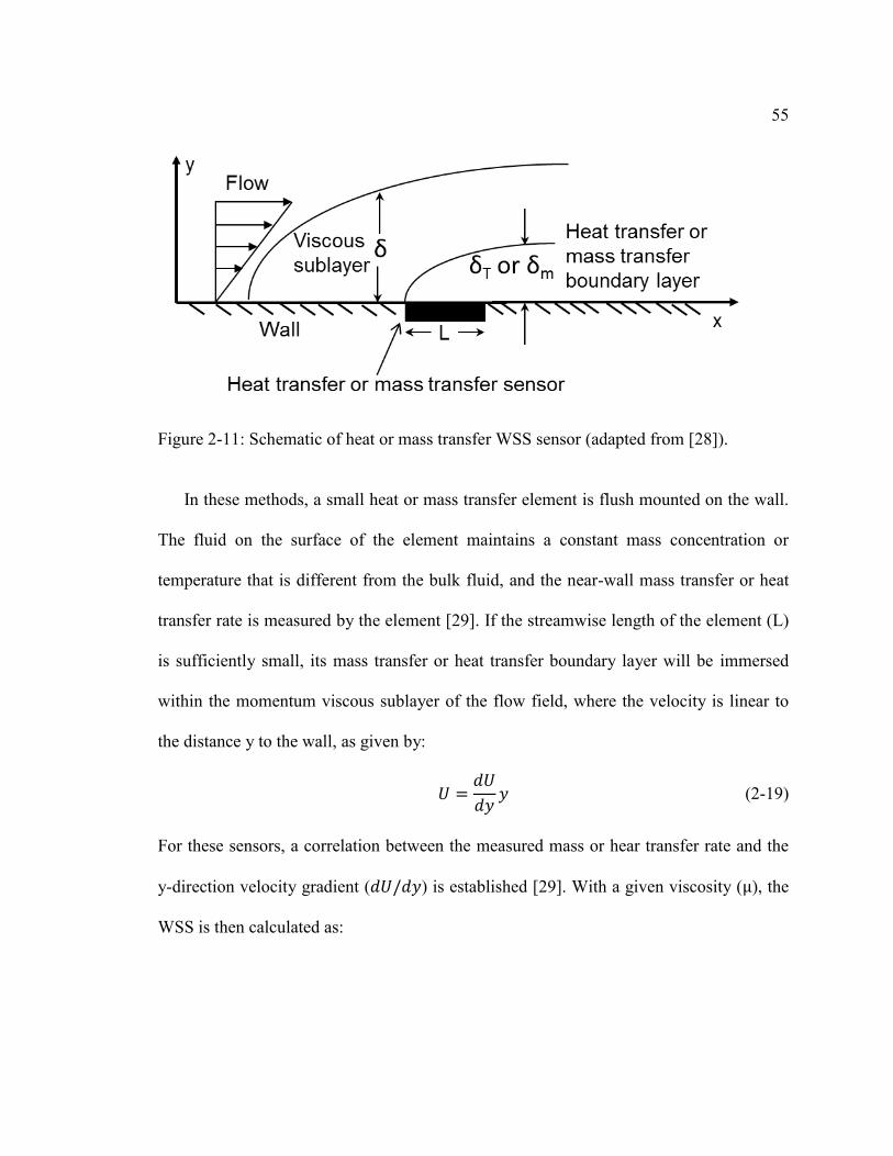
55
Figure 2-11: Schematic of heat or mass transfer WSS sensor (adapted from [28]).
In these methods, a small heat or mass transfer element is flush mounted on the wall.
The fluid on the surface of the element maintains a constant mass concentration or
temperature that is different from the bulk fluid, and the near-wall mass transfer or heat
transfer rate is measured by the element [29]. If the streamwise length of the element (L)
is sufficiently small, its mass transfer or heat transfer boundary layer will be immersed
within the momentum viscous sublayer of the flow field, where the velocity is linear to
the distance y to the wall, as given by:
𝑈 =𝑑𝑈
𝑑𝑦𝑦 (2-19)
For these sensors, a correlation between the measured mass or hear transfer rate and the
y-direction velocity gradient (𝑑𝑈/𝑑𝑦) is established [29]. With a given viscosity (µ), the
WSS is then calculated as:
56
𝜏 = µ𝑑𝑈
𝑑𝑦 (2-20)
Several assumptions need to be satisfied before a correlation can be established, as
commented on by Hanratty and Campbell [29]. For example, the mass/thermal boundary
layer over the sensor element lies within the viscous sub-layer; the diffusion in x
direction can be neglected; and the width of the element is much larger than the mass
transfer boundary layer thickness so that diffusion in the spanwise direction can be
neglected.
The heat transfer sensor is essentially a temperature transducer measuring the heat
transfer rate [28]. Ludwieg and Tillmann [75] used the heat transfer method to measure
the WSS; and they deduced that the heat flux was proportional to the WSS to the power
of 1/3. The heat transfer sensor suffers from a coarse temporal resolution due to the
limited thermal inertia of the element. In addition, an accurate calibration between the
heat transfer rate and WSS is not easily obtained [28].
The electrochemical mass transfer sensor measures the mass transfer limiting current
of an electrochemical reaction that occurs at the surface of the element. The limiting
current is theoretically related to the mass transfer rate as given earlier in Equation
(2-16). Therefore, calibration is not required for this method. By using the Reynolds
analogy, the mass flux is proportional to the 1/3 power of the WSS [29]. The main
disadvantage is that special chemical reagents with high electrochemical reactivity are
needed in an aqueous flow, which is not suitable for studies of gas or pure water flow
[70].

57
2.4.2.3 Methods based on optical techniques
Non-intrusive optical based measurements such as particle image velocimetry
correlate the measured optical properties to the near-wall flow field and provide the WSS
value from theoretical relationships. The principle of optical methods is illustrated in
Figure 2-12.
Figure 2-12: Schematic of laser-based WSS sensor (adapted from [70]).
A laser beam with a wavelength of λ passes through two closely spaced slits (a
distance of d). The diffracted light by the two slits generates interference fringes with a
spacing of δ [70]. The fringe spacing is a function of y-direction distance to the wall, as
given by [70]:
𝛿 =𝜆
𝑑𝑦 (2-21)
When seeding particles are put in the flow, they will scatter light as they pass the fringes,
resulting in Doppler shift of light at the Doppler frequency (𝑓) [70]:
58
𝑓 =𝑈
𝛿 (2-22)
where 𝑈 is the particle velocity. The Doppler scattered light is then recorded by an
optical receiver. If the particles are in the viscous sublayer, the velocity gradient 𝑑𝑈/𝑑𝑦
equals to 𝑈/𝑦 (see Equation (2-19)). Substitution of Equation (2-19), (2-21) and (2-22)
into Equation (2-20) results in:
𝜏 =µ𝑓𝜆
𝑑 (2-23)
Therefore, the WSS can be directly calculated from the measured Doppler frequency,
without the need of calibration. This method allows for instantaneous WSS determination
with a reported high accuracy [28,70]. On the other hand, several disadvantages are
commonly associated with optical-based techniques. For instance, they require
transparent fluids (e.g., air, water) and only work in single-phase flow. In addition, they
are not suitable for measurements in pipes with curved walls.
59
Chapter 3: Research Objectives
The primary objective of this research is to understand the mechanical effects of
multiphase flow on CO2 corrosion inhibition of carbon steel pipelines. The research
focuses on answering the following question, can the hydrodynamic stresses produced by
turbulent multiphase flow alone affect the protective corrosion product layers or
corrosion inhibitor films?
Consequently, wall shear stress, one of the most important forms of mechanical
stresses of flow, has been accurately measured for both single-phase flow and multiphase
flow. In addition, the mechanical effect of extremely turbulent flow on adsorbed inhibitor
films in a CO2 corrosion environment has been investigated by laboratory experiments.
Based on the literature review, research hypotheses were made and have been researched,
as described below.
Hypothesis: Wall shear stress in multiphase flow is directly measurable with a
floating element method. Instead of the more common indirect measurement of the wall
shear stress, direct measurement does not rely on theoretical or empirical correlations
between the WSS and the measured properties. Upon validation, this would be an
effective means to study more complex multiphase flow environments.
Hypothesis: Corrosion product layers or inhibitor films are removed from the steel
surface by high magnitude hydrodynamic stresses (e.g., wall shear stress). It was
hypothesized that, turbulent flow, particularly multiphase flow, with high turbulence and
fluid mixing, generates high mechanical stresses that exceed the adhesion strength of
corrosion product layers or inhibitor films.
60
Hypothesis: Surface geometric irregularity affects local flow conditions, leading to
high instantaneous hydrodynamic stresses, a failure of the corrosion inhibitor film and
pitting corrosion. It was hypothesized that geometric irregularities on the surface of the
pipe, e.g., misalignments, weld beads, bends, tees, etc., significantly alter the local
hydrodynamic conditions and lead to, for example, severe WSS fluctuations. The high
mechanical stresses and fluctuations cause the removal of corrosion product layers and
inhibitor films.
In addition, a critical literature review on the following questions was deemed helpful
for understanding the interaction between flow and corrosion inhibitors:
What is the wall shear stress on an atomic level?
How does flow interfere with the adsorption/desorption processes of inhibitor
molecules?
Better understanding of these questions is important to link the flow (macroscopic) and
the inhibitor molecule adsorption/desorption behavior at the metal surface (microscopic).
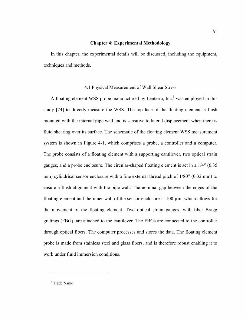
61
Chapter 4: Experimental Methodology
In this chapter, the experimental details will be discussed, including the equipment,
techniques and methods.
4.1 Physical Measurement of Wall Shear Stress
A floating element WSS probe manufactured by Lenterra, Inc.† was employed in this
study [74] to directly measure the WSS. The top face of the floating element is flush
mounted with the internal pipe wall and is sensitive to lateral displacement when there is
fluid shearing over its surface. The schematic of the floating element WSS measurement
system is shown in Figure 4-1, which comprises a probe, a controller and a computer.
The probe consists of a floating element with a supporting cantilever, two optical strain
gauges, and a probe enclosure. The circular-shaped floating element is set in a 1/4″ (6.35
mm) cylindrical sensor enclosure with a fine external thread pitch of 1/80” (0.32 mm) to
ensure a flush alignment with the pipe wall. The nominal gap between the edges of the
floating element and the inner wall of the sensor enclosure is 100 µm, which allows for
the movement of the floating element. Two optical strain gauges, with fiber Bragg
gratings (FBG), are attached to the cantilever. The FBGs are connected to the controller
through optical fibers. The computer processes and stores the data. The floating element
probe is made from stainless steel and glass fibers, and is therefore robust enabling it to
work under fluid immersion conditions.
† Trade Name

62
Figure 4-1: (A) Schematic of a floating element WSS measurement system showing sample measurement; (B) schematic diagram of WSS probe body (by Lenterra with permission).
In principle, direct measurements of WSS rely on accurately measuring the lateral
displacement of the floating element. For this probe, the displacement of the floating
element due to WSS is translated into the changes of optical signals transmitted by the
FBG attached to the cantilever. Any small movement of the element and the consequent
deformation of the cantilever will change the optical reflection spectra from the strain

63
gauges. The optical spectra are processed and provide a WSS value. During a
measurement, the optical controller generates a monochromatic light beam from a laser
diode. This light is directed to the FBG and the reflected light intensity is measured by a
photodiode. The FBG only reflects light at its resonant wavelength and transmits all other
wavelengths, which acts as an optical filter. While tuning the input laser wavelength, the
reflection spectra (reflected light intensity versus laser wavelength) are recorded, from
which the resonant wavelength is determined. The resonant wavelength shifts when the
FBG is strained. Therefore, the WSS causing the displacement of the floating element
and the deflection of the cantilever are represented by the resonant wavelength shift of
the FBG. Temperature change also causes a shift of the resonant wavelength of the FBGs.
Using two FBGs at opposite sides of the cantilever compensates for temperature
sensitivity. When the cantilever is deflected by the flow, FBG1 is stretched and FBG2 is
compressed (Figure 4-1). By subtracting their resonant wavelengths, the difference is
independent of the temperature [74]. The difference between the resonant wavelengths of
the two FBGs due to deflection of the cantilever provides the value of the exerted WSS
on the floating element through the equation:
𝜏 = 𝑘𝛥𝜆 (4-1)
where 𝜏 is the wall shear stress, 𝑘 is a calibration coefficient, and 𝛥𝜆 is the difference
between the resonant wavelengths of the two FBGs. The calibration coefficient is
determined by applying a series of known shear forces to the floating element and
measuring the corresponding values of 𝛥𝜆. The WSS probe comes calibrated from the
supplier.

64
In this study, two floating element WSS probes were used, one with a measurement
range up to 100 Pa and the other with a measurement range up to 1000 Pa. Their nominal
mechanical resonant frequencies are 105 Hz and 235 Hz, respectively. The typical data
acquisition rate of the controller was set to 10k samples/s due to the limitations of the
system hardware. The WSS data recording rate in the computer was set at either 100 Hz
or 1000 Hz by averaging either 100 or 10 samples for each data point. The higher data
recording rate of 1000 Hz provided finer temporal resolution, but also required more
memory from the computer which limited the total recording time. For data recorded at
1000 Hz, a low-pass filter was applied to the raw data to remove the noise from the probe
mechanical resonance. In the flow patterns studied here, no significant difference was
observed when comparing data recorded at 100 Hz and 1000 Hz. Therefore, all the results
reported below are based on data collected at 100 Hz, which allowed longer recording
times.
4.2 Instrumentation and Methods for Flow Tests
In this study, a variety of flow equipment was employed to investigate both single-
phase and multiphase flow patterns.
4.2.1 Equipment for single-phase flow
Single-phase flow experiments were performed in two types of flow geometries:
bounded channel flow and full pipe liquid flow. For channel flow, experiments were
performed in a flow loop with a well-defined flow channel test section, which is referred

65
to as thin channel flow cell (TCFC). Visual representations for TCFC are shown in
Figure 4-2. All wetted parts of the flow loop are made of 316 L stainless steel. A
multistage centrifugal pump is employed to generate the flow. A liquid tank with a
capacity of approximately 40 gallons (151 liters) is used to prepare and store test
solution. The test section is a 600 mm long duct with a rectangular cross-section of 3 mm
high and 89 mm wide. The small cross sectional area of the test section allows the mean
flow velocity to reach up to 17 m/s. The mean volumetric flow is measured by a
paddlewheel flow meter in a 2.54 cm ID (1 inch) pipe section downstream of the test
section. The temperature of the test section and the liquid tank were constantly monitored
by thermocouple probes. For high flow velocity tests, the heat generated in the pump was
removed by a heat exchanger. In the TCFC test section, four ports spaced along the
bottom of the channel are used to flush-mount plug-in probes such as a differential
pressure transducer, wall shear stress measurement probe, electrochemical corrosion
probe and weight loss corrosion specimens.
Figure 4-2: Visual representations of: (A) thin channel flow cell assembly and (B) zoomed-in view of the bottom plate of the test section (top lid not shown).
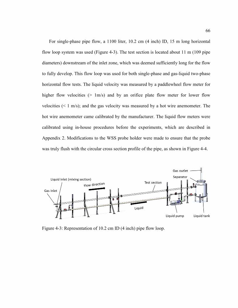
66
For single-phase pipe flow, a 1100 liter, 10.2 cm (4 inch) ID, 15 m long horizontal
flow loop system was used (Figure 4-3). The test section is located about 11 m (109 pipe
diameters) downstream of the inlet zone, which was deemed sufficiently long for the flow
to fully develop. This flow loop was used for both single-phase and gas-liquid two-phase
horizontal flow tests. The liquid velocity was measured by a paddlewheel flow meter for
higher flow velocities (> 1m/s) and by an orifice plate flow meter for lower flow
velocities (< 1 m/s); and the gas velocity was measured by a hot wire anemometer. The
hot wire anemometer came calibrated by the manufacturer. The liquid flow meters were
calibrated using in-house procedures before the experiments, which are described in
Appendix 2. Modifications to the WSS probe holder were made to ensure that the probe
was truly flush with the circular cross section profile of the pipe, as shown in Figure 4-4.
Figure 4-3: Representation of 10.2 cm ID (4 inch) pipe flow loop.
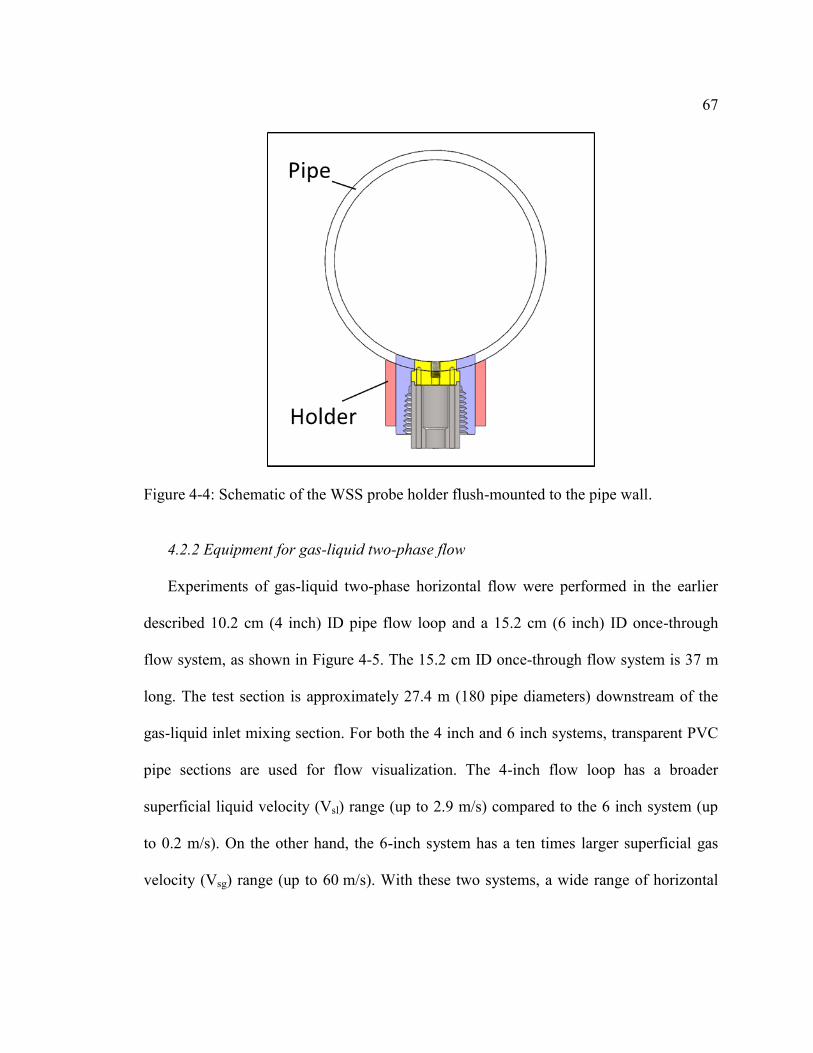
67
Figure 4-4: Schematic of the WSS probe holder flush-mounted to the pipe wall.
4.2.2 Equipment for gas-liquid two-phase flow
Experiments of gas-liquid two-phase horizontal flow were performed in the earlier
described 10.2 cm (4 inch) ID pipe flow loop and a 15.2 cm (6 inch) ID once-through
flow system, as shown in Figure 4-5. The 15.2 cm ID once-through flow system is 37 m
long. The test section is approximately 27.4 m (180 pipe diameters) downstream of the
gas-liquid inlet mixing section. For both the 4 inch and 6 inch systems, transparent PVC
pipe sections are used for flow visualization. The 4-inch flow loop has a broader
superficial liquid velocity (Vsl) range (up to 2.9 m/s) compared to the 6 inch system (up
to 0.2 m/s). On the other hand, the 6-inch system has a ten times larger superficial gas
velocity (Vsg) range (up to 60 m/s). With these two systems, a wide range of horizontal
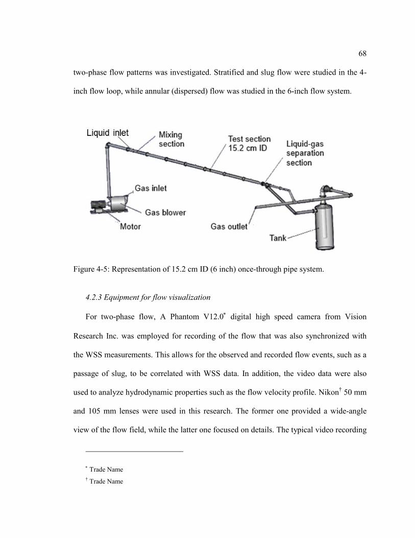
68
two-phase flow patterns was investigated. Stratified and slug flow were studied in the 4-
inch flow loop, while annular (dispersed) flow was studied in the 6-inch flow system.
Figure 4-5: Representation of 15.2 cm ID (6 inch) once-through pipe system.
4.2.3 Equipment for flow visualization
For two-phase flow, A Phantom V12.0 digital high speed camera from Vision
Research Inc. was employed for recording of the flow that was also synchronized with
the WSS measurements. This allows for the observed and recorded flow events, such as a
passage of slug, to be correlated with WSS data. In addition, the video data were also
used to analyze hydrodynamic properties such as the flow velocity profile. Nikon† 50 mm
and 105 mm lenses were used in this research. The former one provided a wide-angle
view of the flow field, while the latter one focused on details. The typical video recording
Trade Name † Trade Name
69
rate was 5000 fps (frames per second). A powerful light source (two 500 W lamps) was
placed behind the pipe test section with a paper light diffuser to provide adequate and
uniform illumination.
4.2.4 Computational fluid dynamics (CFD)
Computational fluid dynamics is a powerful tool for a wide range of physical
modeling processes in fluid mechanics such as turbulence, multiphase flow, heat and
mass transfer, and chemical reactions. In this research, ANSYS Academic Research‡
R 14.0 and R 15.0 were employed for CFD simulations. The CFD results supplemented
the experimental results of wall shear measurement in flow systems and allowed for
estimations of local hydrodynamic properties, which are often not easy to obtain by
experimental measurements.
4.3 Electrochemical Characterization Techniques for Corrosion Tests
Online corrosion measurements were conducted by using a Gamry Reference 600
Potentiostat/Galvanostat/ZRA†. Electrochemical techniques such as open circuit potential
(OCP), linear polarization resistance (LPR), electrochemical impedance spectroscopy
(EIS) and potentiodynamic polarization (PDP) were utilized. The typical parameter
settings for these techniques are given in Table 4-1.
‡ Trade Name † Trade Name
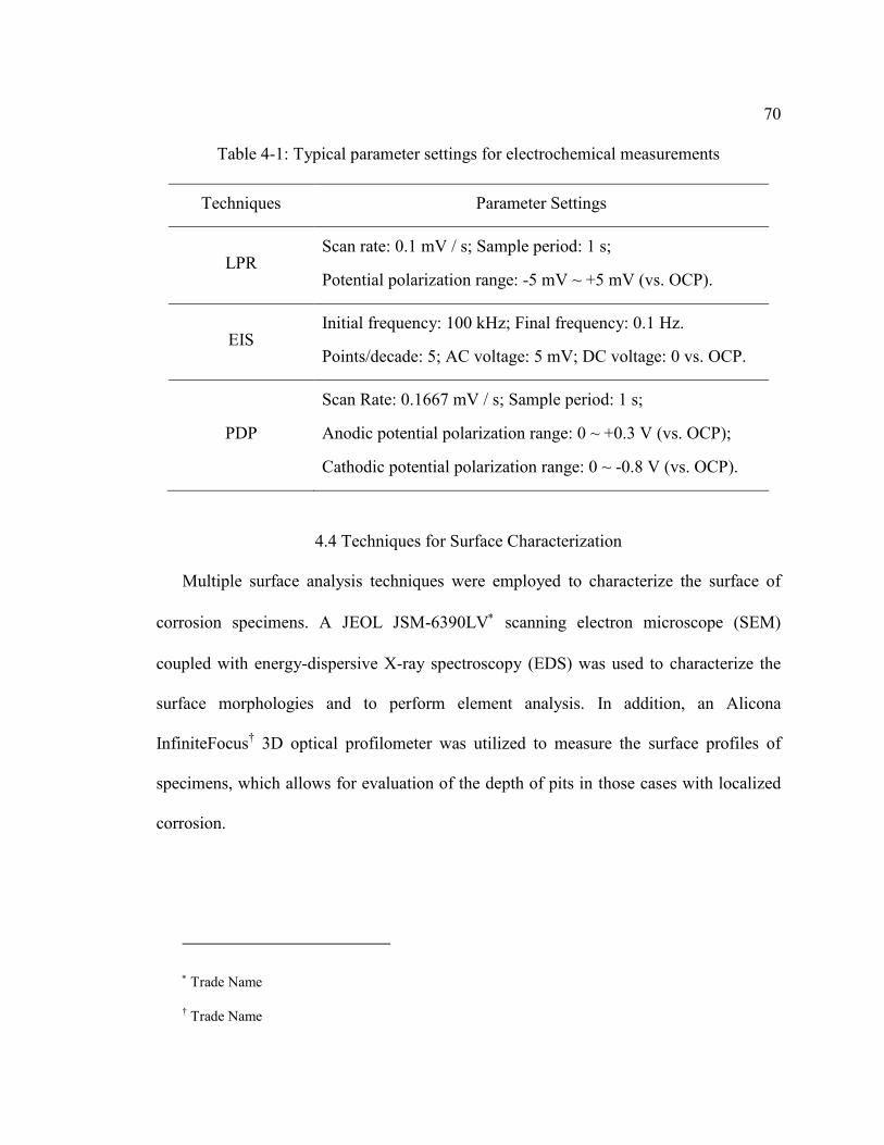
70
Table 4-1: Typical parameter settings for electrochemical measurements
Techniques Parameter Settings
LPR Scan rate: 0.1 mV / s; Sample period: 1 s;
Potential polarization range: -5 mV ~ +5 mV (vs. OCP).
EIS Initial frequency: 100 kHz; Final frequency: 0.1 Hz.
Points/decade: 5; AC voltage: 5 mV; DC voltage: 0 vs. OCP.
PDP
Scan Rate: 0.1667 mV / s; Sample period: 1 s;
Anodic potential polarization range: 0 ~ +0.3 V (vs. OCP);
Cathodic potential polarization range: 0 ~ -0.8 V (vs. OCP).
4.4 Techniques for Surface Characterization
Multiple surface analysis techniques were employed to characterize the surface of
corrosion specimens. A JEOL JSM-6390LV scanning electron microscope (SEM)
coupled with energy-dispersive X-ray spectroscopy (EDS) was used to characterize the
surface morphologies and to perform element analysis. In addition, an Alicona
InfiniteFocus† 3D optical profilometer was utilized to measure the surface profiles of
specimens, which allows for evaluation of the depth of pits in those cases with localized
corrosion.
Trade Name
† Trade Name
71
Chapter 5: Direct Wall Shear Stress Measurements in Gas-Liquid Two-Phase Flow
(Some contents in this chapter were presented in the paper no. 5922 at the NACE
International CORROSION 2015 Conference [76], and have been accepted for
publication in Corrosion Science (In Press) [77].)
5.1 Introduction
The adhesion strength of CO2 corrosion inhibitor films or corrosion product layers to
the steel surface is of the order 1 - 100 MPa, as discussed above. To answer the question
as to whether turbulent flow could mechanically damage the protective inhibitor films or
corrosion product layers, information regarding the magnitude of the hydrodynamic
stresses produced by the flow, particularly wall shear stress (WSS), is required. In this
chapter, single-phase liquid flow and selected, prevalent, gas-liquid two-phase flow
patterns are studied by flow loop experiments; the WSS in these flow patterns are directly
and accurately measured by employing a floating element method.
5.2 Experimental Methodology
In this research, WSS measurements were performed using the floating element WSS
probes (described in Chapter 4) in both single-phase and multiphase flows. Baseline tests
in single-phase flow were done to check the performance of the WSS probe and lay the
groundwork for applications in more complicated flow environments, such as two-phase
flow where accurate WSS predictions were expected to be more difficult.
72
Single-phase flow patterns were studied in the TCFC and the 4-inch pipe loop, while
horizontal gas-liquid two-phase flow patterns were investigated in the 4-inch pipe loop
and the 6-inch flow system (described in Chapter 4). For single-phase flow, WSS was
measured in the bounded channel flow and pipe flow with the test matrix shown in Table
5-1. For two-phase flow patterns, since the phases are not homogeneously distributed
over the pipe cross-section, it was necessary to measure the WSS circumferentially
around the pipe. Consequently, WSS measurements were conducted at three locations on
the pipe wall (bottom, top and side) with the test matrix given in Table 5-2. WSS
measurements were taken with at least one repeat for each flow condition. The summary
of all two-phase flow conditions, for which data were collected, is shown in the context
of a two-phase flow pattern map generated by an in-house gas-liquid flow model [63]
(Figure 5-1). The flow transition lines between stratified-wavy and annular-mist flow for
the 4 inch and 6 inch ID lines, carrying CO2 and air, respectively, are very similar;
therefore, the annular-mist flow data obtained from the 6 inch line was plotted alongside
the data collected in the 4 inch line in the same flow pattern map.
Recorded flow visualization was provided by the earlier described high speed video
camera system in Chapter 4, aiming to contribute to better understanding of the complex
hydrodynamic properties in two-phase flow.
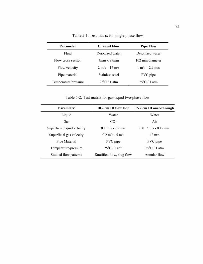
73
Table 5-1: Test matrix for single-phase flow
Parameter Channel Flow Pipe Flow
Fluid Deionized water Deionized water
Flow cross section 3mm x 89mm 102 mm diameter
Flow velocity 2 m/s – 17 m/s 1 m/s – 2.9 m/s
Pipe material Stainless steel PVC pipe
Temperature/pressure 25oC / 1 atm 25oC / 1 atm
Table 5-2: Test matrix for gas-liquid two-phase flow
Parameter 10.2 cm ID flow loop 15.2 cm ID once-through
Liquid Water Water
Gas CO2 Air
Superficial liquid velocity 0.1 m/s - 2.9 m/s 0.017 m/s - 0.17 m/s
Superficial gas velocity 0.2 m/s - 5 m/s 42 m/s
Pipe Material PVC pipe PVC pipe
Temperature/pressure 25oC / 1 atm 25oC / 1 atm
Studied flow patterns Stratified flow, slug flow Annular flow

74
Figure 5-1: Tested flow conditions for WSS measurements in a horizontal two-phase flow pattern map [63] for 1 bar, 25oC, CO2-water, and 4-inch pipe loop.
5.3 Wall Shear Stress Measurements in Single-Phase Flow
To evaluate the validity of WSS measurements made by the floating element probes,
the measured values were compared to empirical well known single-phase correlations
and CFD simulations.
Correlations for calculating mean WSS in single-phase flow are well-established. The
relationship between time-averaged WSS (𝜏) and mean flow velocity for single-phase
flow can be expressed as:
𝜏 =1
2𝜌𝐶𝑓𝑉2 (5-1)
75
where 𝜌 is the fluid density (kg/m3), 𝐶𝑓 is the Fanning friction factor, and 𝑉 is the mean
flow velocity (m/s). The Fanning friction factor is a function of the Reynolds number
(𝑅𝑒) and surface roughness. The Reynolds number is defined as:
𝑅𝑒 =𝜌𝑉𝑑
µ (5-2)
where µ is the dynamic viscosity of the fluid (Pa∙s) and 𝑑 is the hydraulic diameter (m).
For channel flow, the Patel correlation for a smooth surface can be used to calculate
the friction factor [78]:
𝐶𝑓 = 0.0376𝑅𝑒−1/6 (5-3)
The height of channel (h), instead of 2h, was used as the characteristic length to calculate
the Reynolds number as discussed before by Patel et al. [78].
For pipe flow, the Blasius friction factor for a smooth pipe wall was used [78]:
𝐶𝑓 = 0.079𝑅𝑒−1/4 (5-4)
The WSS can be calculated by using the above equations as long as the flow velocity,
pipe dimensions, and fluid properties are determined. The measured WSS from
experiments was compared to the calculated values for both channel and pipe flow. The
mean WSS measured in channel flow shows a reasonably good agreement with the Patel
correlation over a wide range of flow velocities (Figure 5-2). The measurements from
pipe flow are also consistent with the calculated values using the Blasius correlation, as
shown in Figure 5-3. The error bars in the graphs represent the maximum and minimum
values of the WSS measurements.
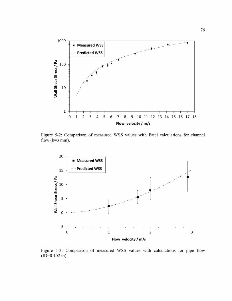
76
Figure 5-2: Comparison of measured WSS values with Patel calculations for channel flow (h=3 mm).
Figure 5-3: Comparison of measured WSS values with calculations for pipe flow (ID=0.102 m).

77
In addition, CFD simulations of the thin channel flow cell were performed. The
simulation geometry is shown in Figure 5-4. As the height of the thin channel (y direction)
is only 3mm, several meshing parameters were adjusted in order to accommodate
sufficient mesh layers in the y direction. Figure 5-5 shows the mesh structure on the x-y
plane in the thin channel. Energy and viscous models were selected to conduct the single-
phase turbulent flow simulations. In the viscous model (turbulent model), the standard k-
epsilon model was selected. The Standard Wall Functions [79] were selected as the near-
wall treatment. After setting up proper boundary conditions, simulations were performed
until all momentum and energy equations converged. Since wall functions were used in
the simulations, the results were checked to ensure that sufficient mesh cells were within
the boundary layers. Simulations with various flow velocities were conducted and
provided calculated WSS values. To illustrate the simulation results by an example,
Figure 5-6 shows the WSS distribution of the four ports at the bottom plate of the TCFC
when the flow velocity is 9.5 m/s. The similarity of the WSS values suggests that the
flow around these port locations is fully developed.
The WSS values obtained from different methods were compared, as shown in Figure
5-7. The error bars in the graph represent the maximum and minimum values of the WSS
using different methods. The agreement for single-phase flow results demonstrates that
the WSS probe had been properly calibrated and was ready for application in two-phase
flow situations.
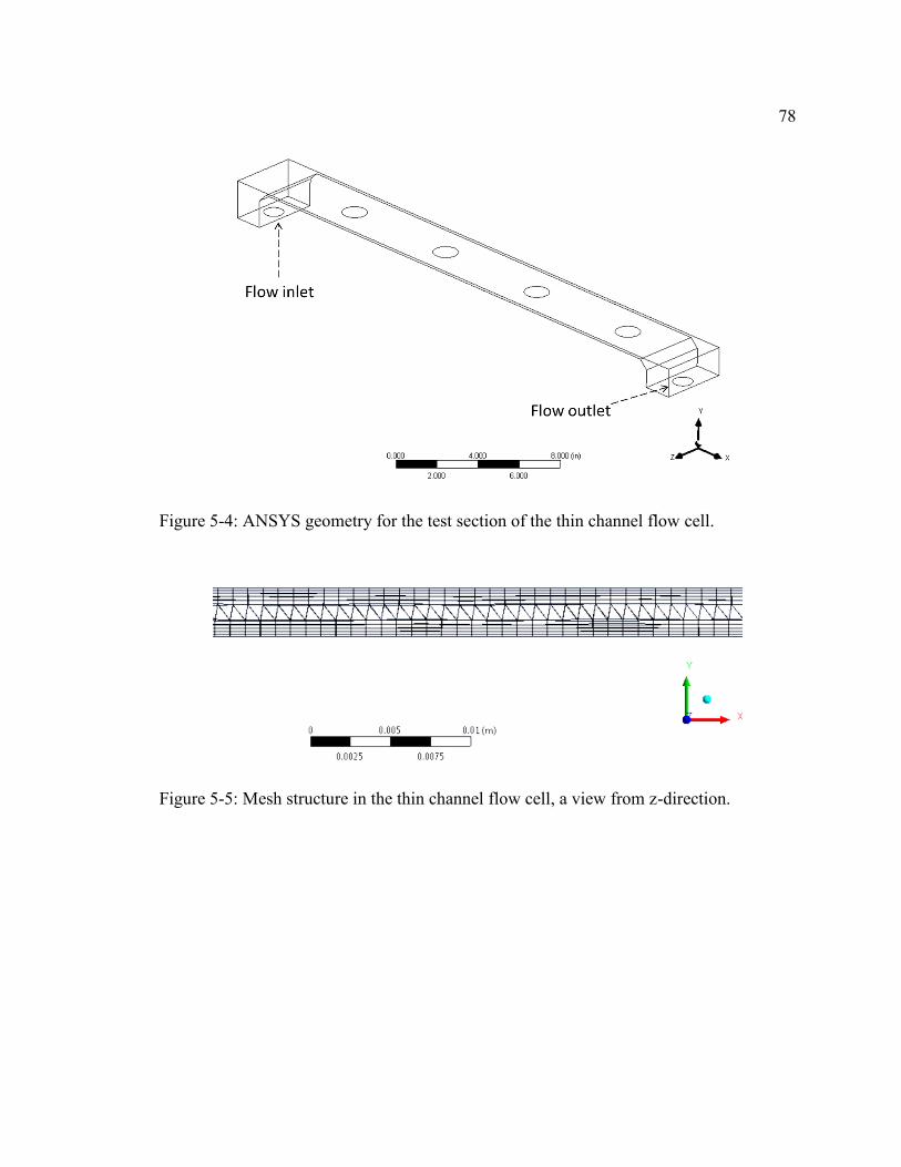
78
Figure 5-4: ANSYS geometry for the test section of the thin channel flow cell.
Figure 5-5: Mesh structure in the thin channel flow cell, a view from z-direction.
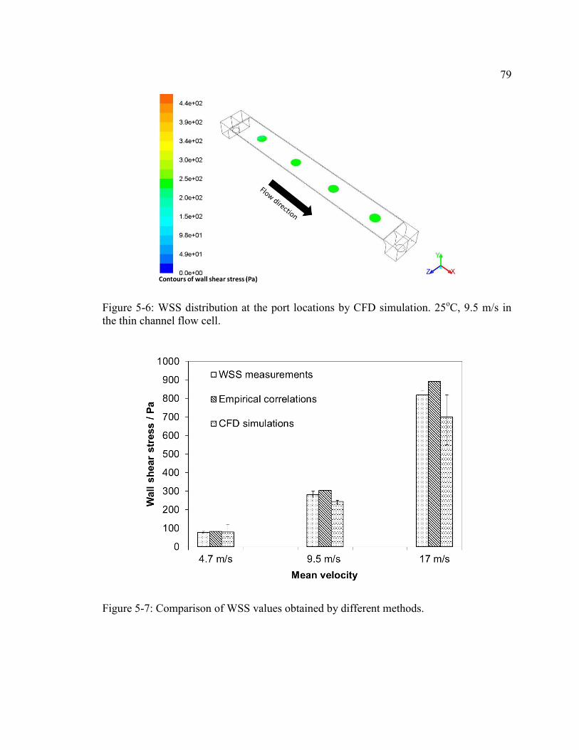
79
Figure 5-6: WSS distribution at the port locations by CFD simulation. 25oC, 9.5 m/s in the thin channel flow cell.
Figure 5-7: Comparison of WSS values obtained by different methods.

80
5.4 Wall Shear Stress Measurements in Gas-Liquid Two-Phase Horizontal Pipe Flow
WSS in multiphase flow exhibits much more complicated behavior compared to
single-phase flow, particularly due to the changes of the liquid phase distribution and
velocity over time and in space. Since there are no well-established WSS correlations for
multiphase flow, direct WSS measurements were seen as a means for contributing to a
better understanding of observed flow-related phenomena.
5.4.1 Wall shear stress measurements in slug flow
Slug flow is considered to be one of the most turbulent multiphase flow patterns [10].
In addition, due to its frequent occurrences in pipelines over a wide range of gas and
liquid flow velocities, understanding the hydrodynamics of slug flow was deemed an
important objective in this study. The features of horizontal slug flow were described
earlier in Figure 2-6. With high turbulence and gas/liquid mixing, the overall slug body
moves at a mixture velocity averaged over the cross-section of the pipe, as given by:
𝑉𝑚 = 𝑉𝑠𝑙 + 𝑉𝑠𝑔 (5-5)
In the stratified zone, a relatively slow liquid film is moving at the bottom, with faster
moving gas above. Due to this inhomogeneous distribution of phases, the WSS values
should be expected to be different around the pipe circumference.
WSS measurements were taken at three locations on the pipe wall (bottom, top and
side). A repeatable procedure was used for measuring WSS at each of these locations. To
illustrate this procedure with an example, Figure 5-8(A) shows the data from a test at
Vsl = 2.0 m/s and Vsg = 2.1 m/s with the WSS probe flush mounted at the bottom of the

81
pipe. A full measurement sequence consists of several steps: (a) the WSS probe started
recording data at 0 s with no flow; (b) the gas was introduced into the flow loop and
reached the required superficial velocity gradually over 10 to 15 s; (c) the liquid was
introduced into the flow loop and reached the specified superficial velocity (data between
the 15 - 20 s markers in Figure 5-8(A)); (d) slug flow became fully developed between 20
- 70 s; (e) the liquid supply was shut off after 70 s; (f) the gas supply was shut off
between 80 - 90 s; and (g) the WSS was recorded for another 10 s in order to confirm that
there was no offset in the measurement from beginning to end. Although the specific
times may vary from test to test, the measurement procedure was the same.
Figure 5-8(B) shows an expanded section of the WSS data taken at the bottom of the
pipe for the fully developed slug flow, covering the time period between the dotted lines
in Figure 5-8(A). The expanded graph shows a series of distinct wall shear stress peaks,
which are presumably corresponding to the passage of slugs.
Figure 5-9 shows a typical WSS measurement at the top of the pipe, which presents a
different pattern, compared to that at the pipe bottom. The WSS peaks are more
pronounced than those seen at the bottom, with much smaller base WSS values in
between. The video data confirmed that the shear stress peaks from both pipe bottom and
top coincided with liquid slug body passages. Three peaks from both Figure 5-8(B) and
Figure 5-9(B) are labeled with time stamps, which will be discussed in the next section.
A number of WSS measurements were taken at the side wall of the pipe, which showed a
similar measurement pattern as seen for the top (as exemplified in Figure 5-10).
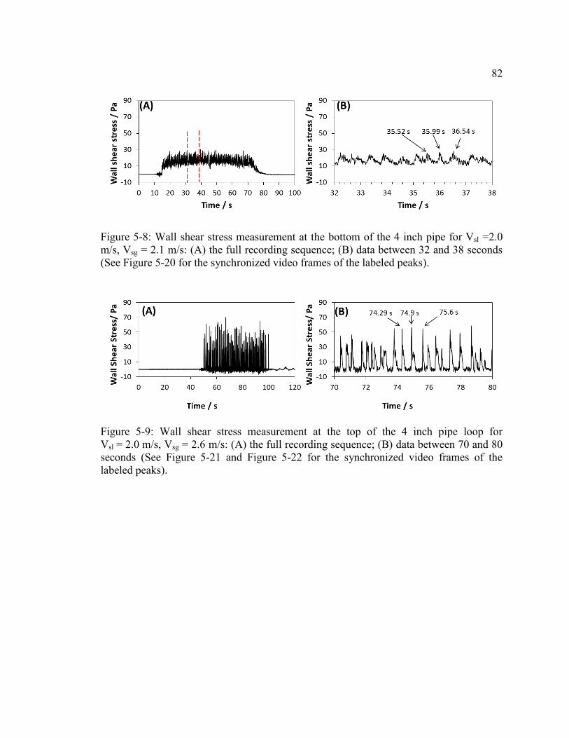
82
Figure 5-8: Wall shear stress measurement at the bottom of the 4 inch pipe for Vsl =2.0 m/s, Vsg = 2.1 m/s: (A) the full recording sequence; (B) data between 32 and 38 seconds (See Figure 5-20 for the synchronized video frames of the labeled peaks).
Figure 5-9: Wall shear stress measurement at the top of the 4 inch pipe loop for Vsl = 2.0 m/s, Vsg = 2.6 m/s: (A) the full recording sequence; (B) data between 70 and 80 seconds (See Figure 5-21 and Figure 5-22 for the synchronized video frames of the labeled peaks).

83
Figure 5-10: Wall shear stress measurement at the sidewall of the 4 inch pipe loop for Vsl = 0.3 m/s, Vsg = 2.6 m/s: (A) the full recording sequence; (B) data between 160 and 200 seconds.
The different patterns of the WSS data taken for different locations of the pipe
circumference can be easily explained by the characteristics of horizontal slug flow.
When the WSS probe was at the bottom, it was constantly immersed in a moving liquid
phase, either in the form of a stratified film or a liquid slug body. As shown in Figure
5-8(B), the base WSS value of about 15 Pa was due to the movement of the stratified film
between the slugs, which caused peak WSS up to 29 Pa. On the other hand, when the
WSS probe was at the top, there was a measurable WSS only when the liquid slug body
was bridging the entire pipe cross-section as it passed over the probe. Without the liquid
slug, the gas phase exerted a negligible WSS on the probe, due to its low density as
compared to the liquid phase. This is evident by the WSS data shown in Figure 5-9(B)
where the measured WSS was almost zero between peaks, when no liquid slug body was
present. The patterns of the WSS data at the sidewall suggest that the height of the liquid
phase in the stratified film zone was much lower than the probe location, and WSS was
recorded only when the liquid slug zone passed the probe. This is a reasonable
84
explanation as the liquid velocities were relatively low for WSS measurements at the
sidewall of the pipe.
It was generally found that an increasing mixture velocity leads to an increasing WSS
value at each of the probe locations. The maximum WSS values measured at the bottom,
top, and side of the pipe for each condition are tabulated in Table 5-3. The maximum
WSS value was determined by averaging the largest 20 values for each flow condition, in
order to get a more representative value that can be used for modeling. To demonstrate
this increase in WSS with increasing mixture velocity, Figure 5-11 to Figure 5-13 show
the maximum WSS value measured for each condition around the pipe circumference,
overlain with the corresponding two-phase flow pattern map. It should be noted that in
some of the test conditions stratified flow was predicted by the flow pattern map, while it
was actually slug flow (Figure 5-11) as confirmed by the video data. This is probably due
to these conditions being close to the transition line between stratified flow and slug flow,
and the inherent inaccuracy of the model used. Similarly, the maximum WSS values for
tests at Vsl = 2.9 m/s, Vsg = 0.2 m/s and 0.6 m/s were unreported (Figure 5-12), as
transitions between slug flow and dispersed-bubble flow were observed from the video
data.

85
Table 5-3: Wall shear stress measurements for slug flow in the 4 inch pipe loop
Probe location
Vsl / (m/s)
Vsg / (m/s)
Vm / (m/s)
Max WSS / (Pa)
Bottom 0.1 0.2 0.3 1 Bottom 0.1 0.6 0.7 2 Bottom 0.1 2.6 2.7 7 Bottom 0.2 0.6 0.8 2 Bottom 0.2 2.6 2.8 8 Bottom 0.3 0.2 0.5 1 Bottom 0.3 0.6 0.9 2 Bottom 0.3 2.6 2.9 10 Bottom 1.0 0.6 1.6 9 Bottom 1.0 1.3 2.3 12 Bottom 1.0 2.1 3.1 23 Bottom 1.0 2.6 3.6 22 Bottom 1.0 5.0 6 35 Bottom 2.0 0.6 2.6 24 Bottom 2.0 1.3 3.3 27 Bottom 2.0 2.1 4.1 28 Bottom 2.0 2.6 4.6 27 Bottom 2.9 1.3 4.2 29 Bottom 2.9 2.1 5.0 34 Bottom 2.9 2.6 5.5 38 Bottom 2.9 5.0 7.9 54
Top 0.1 0.6 0.7 18 Top 0.1 2.6 2.7 31 Top 0.2 2.6 2.8 41 Top 0.3 0.6 0.9 22 Top 0.3 2.6 2.9 36 Top 1.0 2.6 3.6 52 Top 1.0 5.0 6 75 Top 2.0 2.6 4.6 58 Top 2.0 5.0 7.0 79 Top 2.9 2.6 5.5 59 Top 2.9 5.0 7.9 80 Side 0.1 0.6 0.7 5 Side 0.1 2.6 2.7 17 Side 0.2 2.6 2.8 21 Side 0.3 0.6 0.9 10 Side 0.3 2.6 2.9 32

86
Figure 5-11: 𝜏max (Pa) shown next to markers for slug flow measured at the bottom of the pipe overlain with the flow pattern map [63], at 1 bar, 25oC, CO2-water, and in the 4-inch loop.
Figure 5-12: 𝜏max (Pa) shown next to markers for slug flow measured at the top of the pipe overlain with the flow pattern map [63], at 1 bar, 25oC, CO2-water, and in the 4-inch loop.
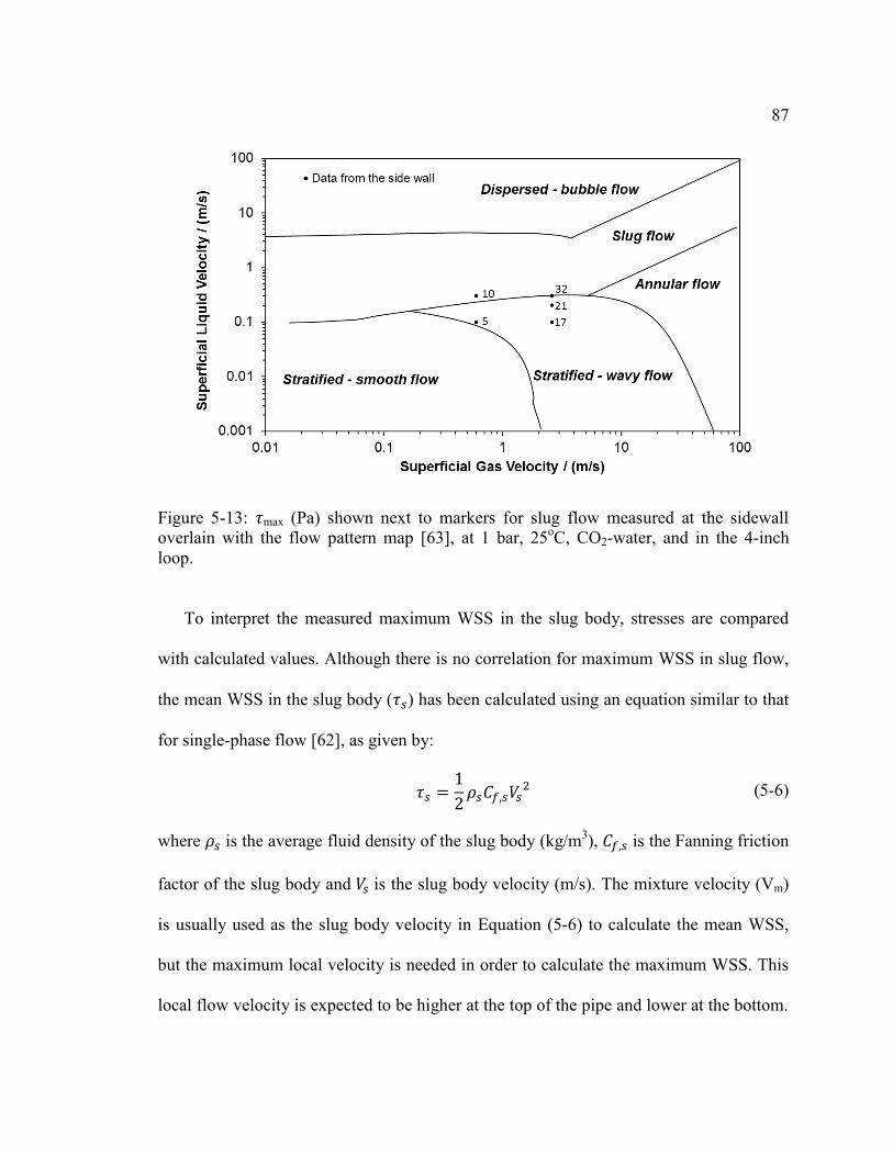
87
Figure 5-13: 𝜏max (Pa) shown next to markers for slug flow measured at the sidewall overlain with the flow pattern map [63], at 1 bar, 25oC, CO2-water, and in the 4-inch loop.
To interpret the measured maximum WSS in the slug body, stresses are compared
with calculated values. Although there is no correlation for maximum WSS in slug flow,
the mean WSS in the slug body (𝜏𝑠) has been calculated using an equation similar to that
for single-phase flow [62], as given by:
𝜏𝑠 =1
2𝜌𝑠𝐶𝑓,𝑠𝑉𝑠
2 (5-6)
where 𝜌𝑠 is the average fluid density of the slug body (kg/m3), 𝐶𝑓,𝑠 is the Fanning friction
factor of the slug body and 𝑉𝑠 is the slug body velocity (m/s). The mixture velocity (Vm)
is usually used as the slug body velocity in Equation (5-6) to calculate the mean WSS,
but the maximum local velocity is needed in order to calculate the maximum WSS. This
local flow velocity is expected to be higher at the top of the pipe and lower at the bottom.
88
To calculate the friction factor in Equation (5-6), the Blasius-type correlation for smooth
pipes was used:
𝐶𝑓,𝑠 = 0.079𝑅𝑒𝑠−1/4 (5-7)
where the Reynolds number of the slug body (𝑅𝑒𝑠) using the pipe diameter (𝐷) was
written as:
𝑅𝑒𝑠 =𝜌𝑠𝐷𝑉𝑠
𝜇𝑠 (5-8)
The average slug body density (𝜌𝑠) and viscosity (𝜇𝑠) were calculated as:
𝜌𝑠 = 𝜌𝐿𝐻𝑙𝑠 + 𝜌𝐺(1 − 𝐻𝑙𝑠) (5-9)
𝜇𝑠 = 𝜇𝐿𝐻𝑙𝑠 + 𝜇𝐺(1 − 𝐻𝑙𝑠) (5-10)
where 𝜌𝐿 and 𝜇𝐿 are the liquid density and viscosity, 𝜌𝐺 and 𝜇𝐺 are the gas density and
viscosity, and 𝐻𝑙𝑠 is the slug liquid holdup. A correlation for horizontal flow by
Gregory et al. [80] was used to calculate the slug liquid holdup:
𝐻𝑙𝑠 =1
1 + (𝑉𝑚
8.66)1.39 (5-11)
By using Equation (5-6) through Equation (5-11), the slug WSS can be calculated using
the average slug body density and viscosity and a defined slug body velocity, as given by:
𝜏𝑠 = 0.0395 ∙ 𝐷−0.25𝜌𝑠0.75𝜇𝑠
0.25𝑉𝑠1.75 (5-12)
The mean WSS of the slug body is compared with the measured maximum WSS for
each flow condition in Figure 5-14. Generally, the measured maximum WSS values for
all probe locations are higher than the calculated values when using the mixture velocity.
This finding is important as many slug flow models only calculate the mean shear stress
of the slug body by using the mixture velocity, which can underestimate the maximum

89
WSS by a large margin (a factor of 2-4). The finding also indicates that the highest WSS
value occurred when the liquid slug passed the probe with a local velocity being higher
than the mixture velocity. In addition, it was found that at the same flow condition, the
maximum WSS at the top of the pipe was higher than that measured at the bottom of the
pipe, while the maximum WSS measured at the sidewall was an intermediate value. It
was assumed that the difference among the maximum WSS values at these three probe
locations was due to the variation of the local liquid flow velocity in the slug body. In
other words, the top part of the slug body had a higher maximum flow velocity than the
bottom part of the slug body.
Figure 5-14: Comparison between measured maximum WSS values and calculated mean slug WSS values from Equation (5-12) by using mixture velocity (Vm), for 4-inch loop.

90
To better predict the maximum WSS, the maximum local velocity in the slug body
was required. The in situ local velocity of the liquid in the slug body was determined
using video data, as illustrated in Figure 5-15. Two images of a liquid slug with a small
time separation Δt (0.003 s) were compared. To determine actual liquid velocities, small
gas bubbles, entrained by the liquid, were used as tracers to determine liquid velocities.
For example, using Figure 5-15, the in situ liquid velocity at the pipe top near the slug
front was calculated as Δx1/Δt. For low-quality images, the slug nose interface near the
top was used as a tracer to estimate the liquid velocity. It should be noted that this
interface velocity, or slug translational velocity, is not an actual liquid velocity. Because
of the scooping up of the liquid from the stratified film into the slug body, the
translational velocity is higher than the mixture velocity. Nevertheless, the translational
velocity was deemed the maximum possible local velocity in the slug body [62].
Similarly, by tracking the horizontal movement of a small gas bubble in the slug body
near the pipe bottom (Δx2), the local liquid velocity at the pipe bottom was calculated as
Δx2/Δt.
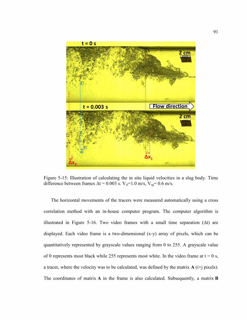
91
Figure 5-15: Illustration of calculating the in situ liquid velocities in a slug body. Time difference between frames Δt = 0.003 s. Vsl=1.0 m/s, Vsg= 0.6 m/s.
The horizontal movements of the tracers were measured automatically using a cross
correlation method with an in-house computer program. The computer algorithm is
illustrated in Figure 5-16. Two video frames with a small time separation (Δt) are
displayed. Each video frame is a two-dimensional (x-y) array of pixels, which can be
quantitatively represented by grayscale values ranging from 0 to 255. A grayscale value
of 0 represents most black while 255 represents most white. In the video frame at t = 0 s,
a tracer, where the velocity was to be calculated, was defined by the matrix A (i×j pixels).
The coordinates of matrix A in the frame is also calculated. Subsequently, a matrix B
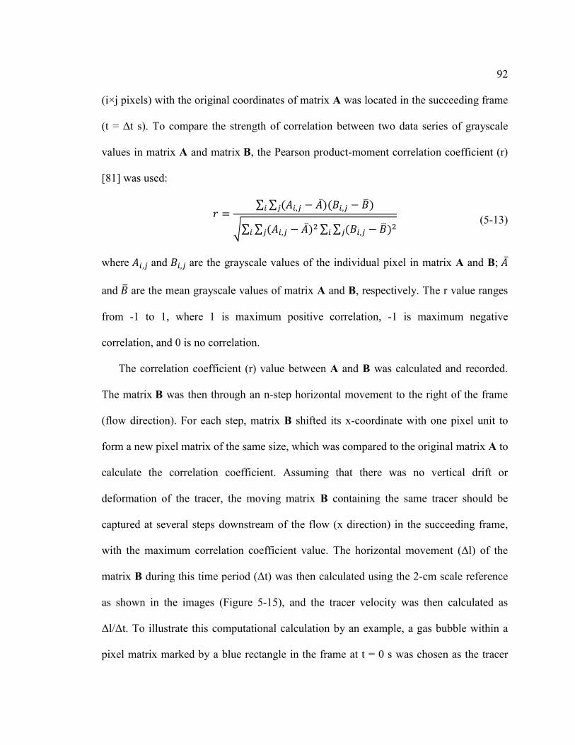
92
(i×j pixels) with the original coordinates of matrix A was located in the succeeding frame
(t = Δt s). To compare the strength of correlation between two data series of grayscale
values in matrix A and matrix B, the Pearson product-moment correlation coefficient (r)
[81] was used:
𝑟 =∑ ∑ (𝐴𝑖,𝑗 − �̅�)(𝐵𝑖,𝑗 − �̅�)𝑗𝑖
√∑ ∑ (𝐴𝑖,𝑗 − �̅�)2𝑗𝑖 ∑ ∑ (𝐵𝑖,𝑗 − �̅�)2
𝑗𝑖
(5-13)
where 𝐴𝑖,𝑗 and 𝐵𝑖,𝑗 are the grayscale values of the individual pixel in matrix A and B; �̅�
and �̅� are the mean grayscale values of matrix A and B, respectively. The r value ranges
from -1 to 1, where 1 is maximum positive correlation, -1 is maximum negative
correlation, and 0 is no correlation.
The correlation coefficient (r) value between A and B was calculated and recorded.
The matrix B was then through an n-step horizontal movement to the right of the frame
(flow direction). For each step, matrix B shifted its x-coordinate with one pixel unit to
form a new pixel matrix of the same size, which was compared to the original matrix A to
calculate the correlation coefficient. Assuming that there was no vertical drift or
deformation of the tracer, the moving matrix B containing the same tracer should be
captured at several steps downstream of the flow (x direction) in the succeeding frame,
with the maximum correlation coefficient value. The horizontal movement (Δl) of the
matrix B during this time period (Δt) was then calculated using the 2-cm scale reference
as shown in the images (Figure 5-15), and the tracer velocity was then calculated as
Δl/Δt. To illustrate this computational calculation by an example, a gas bubble within a
pixel matrix marked by a blue rectangle in the frame at t = 0 s was chosen as the tracer
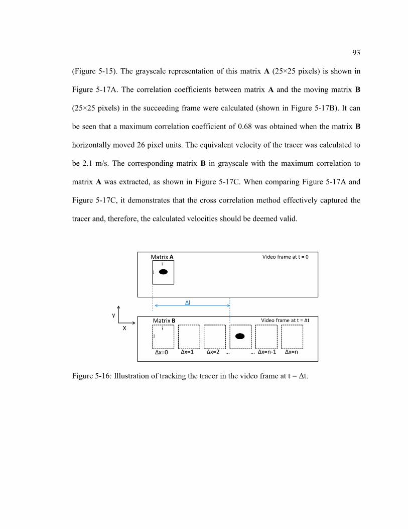
93
(Figure 5-15). The grayscale representation of this matrix A (25×25 pixels) is shown in
Figure 5-17A. The correlation coefficients between matrix A and the moving matrix B
(25×25 pixels) in the succeeding frame were calculated (shown in Figure 5-17B). It can
be seen that a maximum correlation coefficient of 0.68 was obtained when the matrix B
horizontally moved 26 pixel units. The equivalent velocity of the tracer was calculated to
be 2.1 m/s. The corresponding matrix B in grayscale with the maximum correlation to
matrix A was extracted, as shown in Figure 5-17C. When comparing Figure 5-17A and
Figure 5-17C, it demonstrates that the cross correlation method effectively captured the
tracer and, therefore, the calculated velocities should be deemed valid.
Figure 5-16: Illustration of tracking the tracer in the video frame at t = Δt.
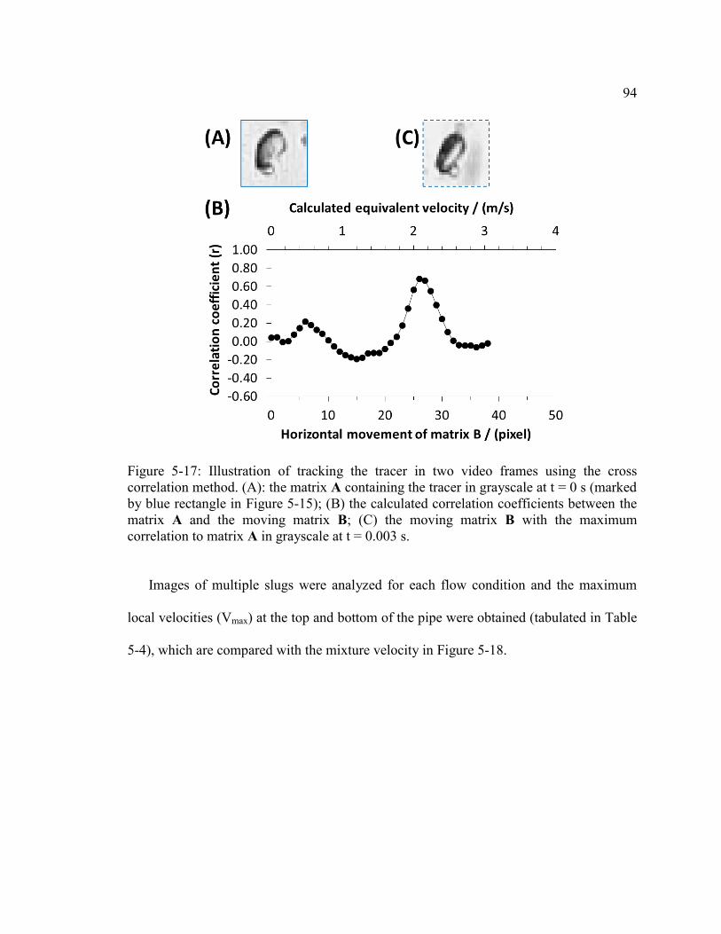
94
Figure 5-17: Illustration of tracking the tracer in two video frames using the cross correlation method. (A): the matrix A containing the tracer in grayscale at t = 0 s (marked by blue rectangle in Figure 5-15); (B) the calculated correlation coefficients between the matrix A and the moving matrix B; (C) the moving matrix B with the maximum correlation to matrix A in grayscale at t = 0.003 s.
Images of multiple slugs were analyzed for each flow condition and the maximum
local velocities (Vmax) at the top and bottom of the pipe were obtained (tabulated in Table
5-4), which are compared with the mixture velocity in Figure 5-18.
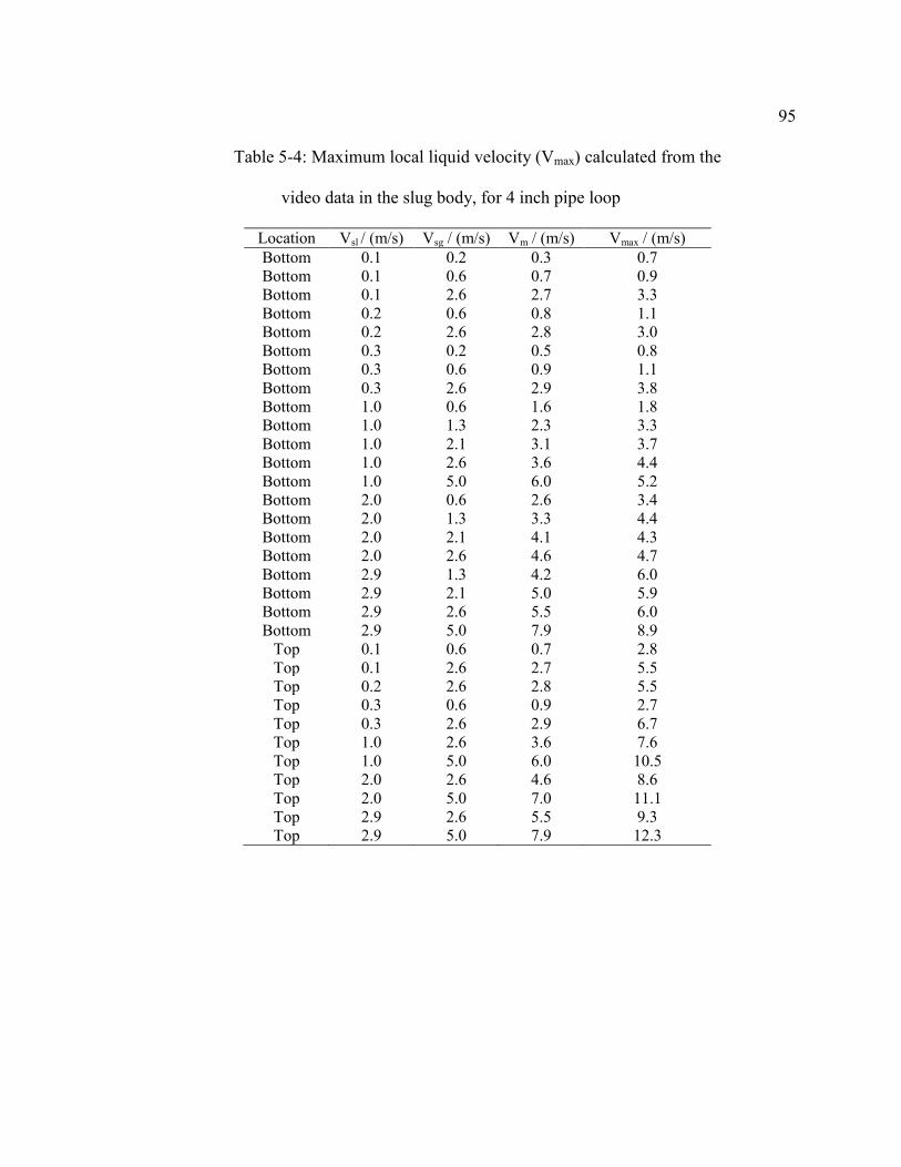
95
Table 5-4: Maximum local liquid velocity (Vmax) calculated from the
video data in the slug body, for 4 inch pipe loop
Location Vsl / (m/s) Vsg / (m/s) Vm / (m/s) Vmax / (m/s) Bottom 0.1 0.2 0.3 0.7 Bottom 0.1 0.6 0.7 0.9 Bottom 0.1 2.6 2.7 3.3 Bottom 0.2 0.6 0.8 1.1 Bottom 0.2 2.6 2.8 3.0 Bottom 0.3 0.2 0.5 0.8 Bottom 0.3 0.6 0.9 1.1 Bottom 0.3 2.6 2.9 3.8 Bottom 1.0 0.6 1.6 1.8 Bottom 1.0 1.3 2.3 3.3 Bottom 1.0 2.1 3.1 3.7 Bottom 1.0 2.6 3.6 4.4 Bottom 1.0 5.0 6.0 5.2 Bottom 2.0 0.6 2.6 3.4 Bottom 2.0 1.3 3.3 4.4 Bottom 2.0 2.1 4.1 4.3 Bottom 2.0 2.6 4.6 4.7 Bottom 2.9 1.3 4.2 6.0 Bottom 2.9 2.1 5.0 5.9 Bottom 2.9 2.6 5.5 6.0 Bottom 2.9 5.0 7.9 8.9
Top 0.1 0.6 0.7 2.8 Top 0.1 2.6 2.7 5.5 Top 0.2 2.6 2.8 5.5 Top 0.3 0.6 0.9 2.7 Top 0.3 2.6 2.9 6.7 Top 1.0 2.6 3.6 7.6 Top 1.0 5.0 6.0 10.5 Top 2.0 2.6 4.6 8.6 Top 2.0 5.0 7.0 11.1 Top 2.9 2.6 5.5 9.3 Top 2.9 5.0 7.9 12.3
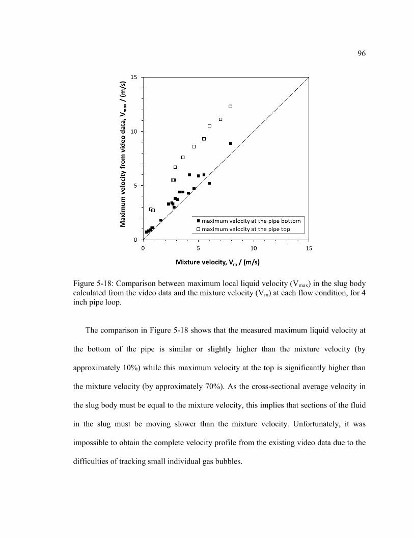
96
Figure 5-18: Comparison between maximum local liquid velocity (Vmax) in the slug body calculated from the video data and the mixture velocity (Vm) at each flow condition, for 4 inch pipe loop.
The comparison in Figure 5-18 shows that the measured maximum liquid velocity at
the bottom of the pipe is similar or slightly higher than the mixture velocity (by
approximately 10%) while this maximum velocity at the top is significantly higher than
the mixture velocity (by approximately 70%). As the cross-sectional average velocity in
the slug body must be equal to the mixture velocity, this implies that sections of the fluid
in the slug must be moving slower than the mixture velocity. Unfortunately, it was
impossible to obtain the complete velocity profile from the existing video data due to the
difficulties of tracking small individual gas bubbles.
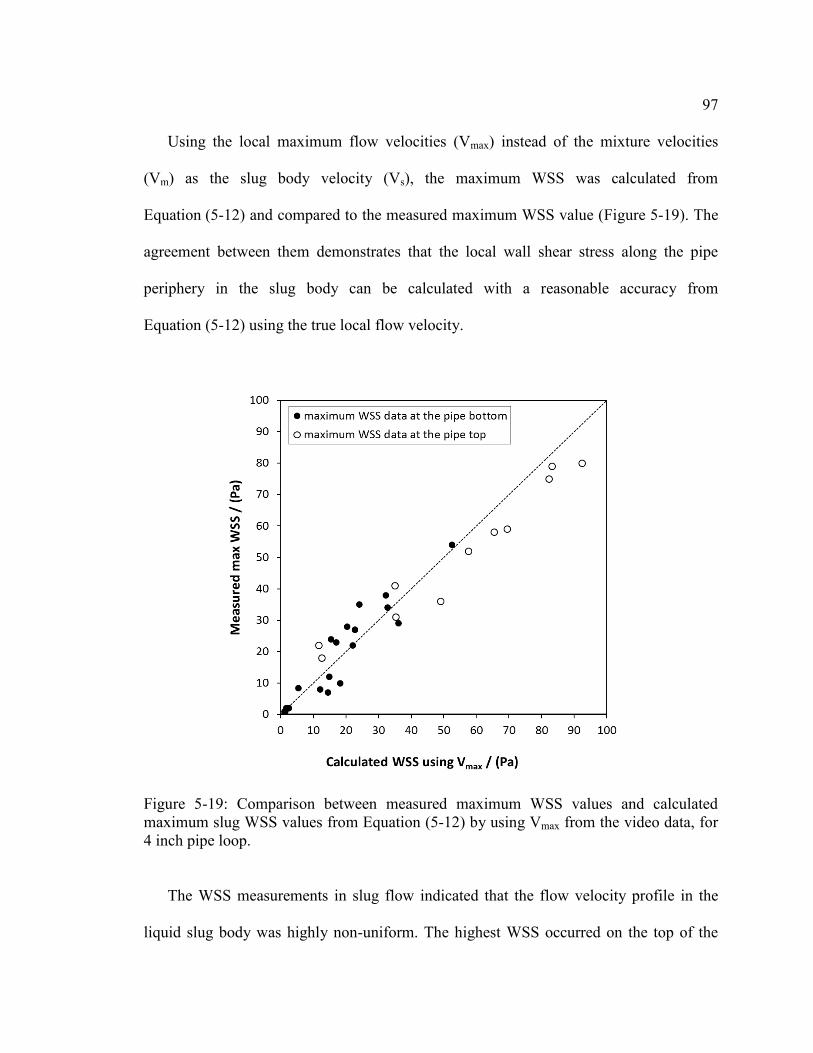
97
Using the local maximum flow velocities (Vmax) instead of the mixture velocities
(Vm) as the slug body velocity (Vs), the maximum WSS was calculated from
Equation (5-12) and compared to the measured maximum WSS value (Figure 5-19). The
agreement between them demonstrates that the local wall shear stress along the pipe
periphery in the slug body can be calculated with a reasonable accuracy from
Equation (5-12) using the true local flow velocity.
Figure 5-19: Comparison between measured maximum WSS values and calculated maximum slug WSS values from Equation (5-12) by using Vmax from the video data, for 4 inch pipe loop.
The WSS measurements in slug flow indicated that the flow velocity profile in the
liquid slug body was highly non-uniform. The highest WSS occurred on the top of the

98
pipe when the slug front passed with the maximum in situ flow velocity. The maximum
WSS value was about 2 to 4 times higher than the calculated mean WSS value from
empirical correlations when using the mixture velocity; this may serve as a guideline for
operations involving slug flow and for slug modeling with applications to other areas,
such as removal of corrosion inhibitor films and corrosion product layers.
5.4.2 Assessment of the location with the highest wall shear stress in a slug
In order to investigate the relationship between WSS measurements and flow
patterns, a synchronized high speed camera was used in tandem with the shear stress
probe. This was to assess which part of the liquid slug body would generate the highest
WSS. Figure 5-20 shows flow visualization frames of passing slug bodies corresponding
to the WSS peak values that occur at 35.52 s, 35.99 s, and 36.54 s, as marked in Figure
5-8(B), respectively. In the images the WSS probe was masked by the black opaque
probe holder and was flush mounted to the bottom pipe wall (at location “1” in Figure
5-20; also see Figure 4-4). A 2 cm tape was attached to the front pipe wall as a length
scale reference (marked as “2” in Figure 5-20). In this specific flow condition, for the
peaks at 35.52 s and 35.99 s, the highest bottom WSS value was recorded at exactly the
same time when the slug front passed the WSS probe. However, for the peak at 36.54 s,
the highest WSS was measured in the middle of the slug body. Considering all flow
conditions documented by direct WSS measurement and high speed video recordings, no
clear correlation was observed between the maximum WSS and a specific location in the
slug body when the probe was at the bottom of the pipe. This can be explained by the
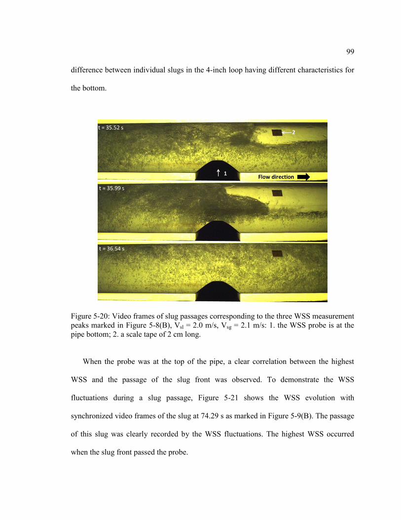
99
difference between individual slugs in the 4-inch loop having different characteristics for
the bottom.
Figure 5-20: Video frames of slug passages corresponding to the three WSS measurement peaks marked in Figure 5-8(B), Vsl = 2.0 m/s, Vsg = 2.1 m/s: 1. the WSS probe is at the pipe bottom; 2. a scale tape of 2 cm long.
When the probe was at the top of the pipe, a clear correlation between the highest
WSS and the passage of the slug front was observed. To demonstrate the WSS
fluctuations during a slug passage, Figure 5-21 shows the WSS evolution with
synchronized video frames of the slug at 74.29 s as marked in Figure 5-9(B). The passage
of this slug was clearly recorded by the WSS fluctuations. The highest WSS occurred
when the slug front passed the probe.

100
Figure 5-21: Evolution of the WSS fluctuations with synchronized video frames of the slug around 74.29 s marked in Figure 5-9(B), Vsl = 2.0 m/s, Vsg = 2.6 m/s, 4 inch pipe.
Figure 5-22 shows flow image frames corresponding to the three consecutive WSS
peaks shown in Figure 5-9(B). In this condition, the WSS peak values were always
recorded at a time shortly after the slug fronts passed the WSS probe. This observation
was repeatable and consistent for all slugs. This finding confirms that the slug front
generates the highest WSS at the top of the pipe irrespective of flow condition.
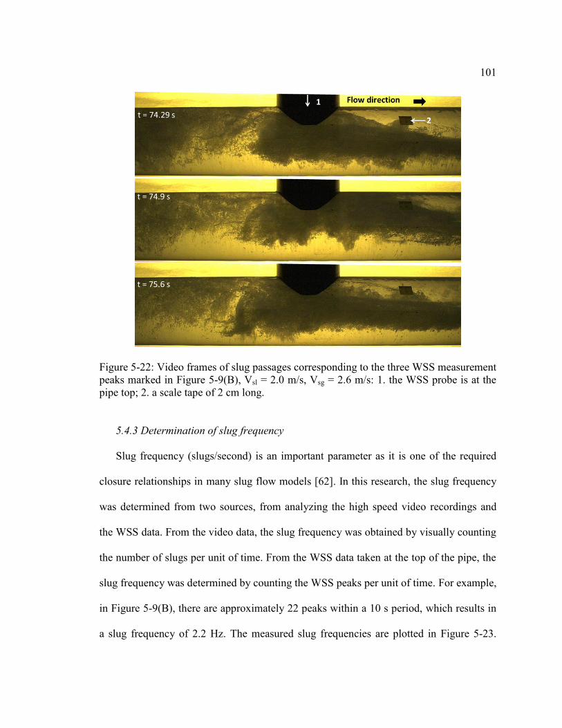
101
Figure 5-22: Video frames of slug passages corresponding to the three WSS measurement peaks marked in Figure 5-9(B), Vsl = 2.0 m/s, Vsg = 2.6 m/s: 1. the WSS probe is at the pipe top; 2. a scale tape of 2 cm long.
5.4.3 Determination of slug frequency
Slug frequency (slugs/second) is an important parameter as it is one of the required
closure relationships in many slug flow models [62]. In this research, the slug frequency
was determined from two sources, from analyzing the high speed video recordings and
the WSS data. From the video data, the slug frequency was obtained by visually counting
the number of slugs per unit of time. From the WSS data taken at the top of the pipe, the
slug frequency was determined by counting the WSS peaks per unit of time. For example,
in Figure 5-9(B), there are approximately 22 peaks within a 10 s period, which results in
a slug frequency of 2.2 Hz. The measured slug frequencies are plotted in Figure 5-23.
102
Both methods should and did give almost the same results. The slug frequency increases
with increasing superficial liquid velocity, and slightly decreases with increasing
superficial gas velocity. The measured slug frequencies were compared with the data of
Heywood and Richardson at similar flow conditions in a 42 mm ID (1.65 inch) pipe [82],
as shown in Figure 5-23. The results are coherent for these two sets of data despite the
fact they were obtained in different pipe diameter systems. Existing literature reports that
a minimum slug frequency exists as a function of Vsg for a given Vsl [82–84]. Gregory
and Scott reported slug frequency data with a Vsl up to 1.3 m/s, and found the minima
occurred at a slug translational velocity of approximately 6 m/s for each Vsl [84]. Woods
et al. [83] found the minimum slug frequency to be at approximately Vsg = 4 m/s in a
0.095 m ID pipe for data with Vsl up to 1.2 m/s. In the present study no clear minimum
was observed, which may be due to the narrow gas velocity range (up to 5 m/s).
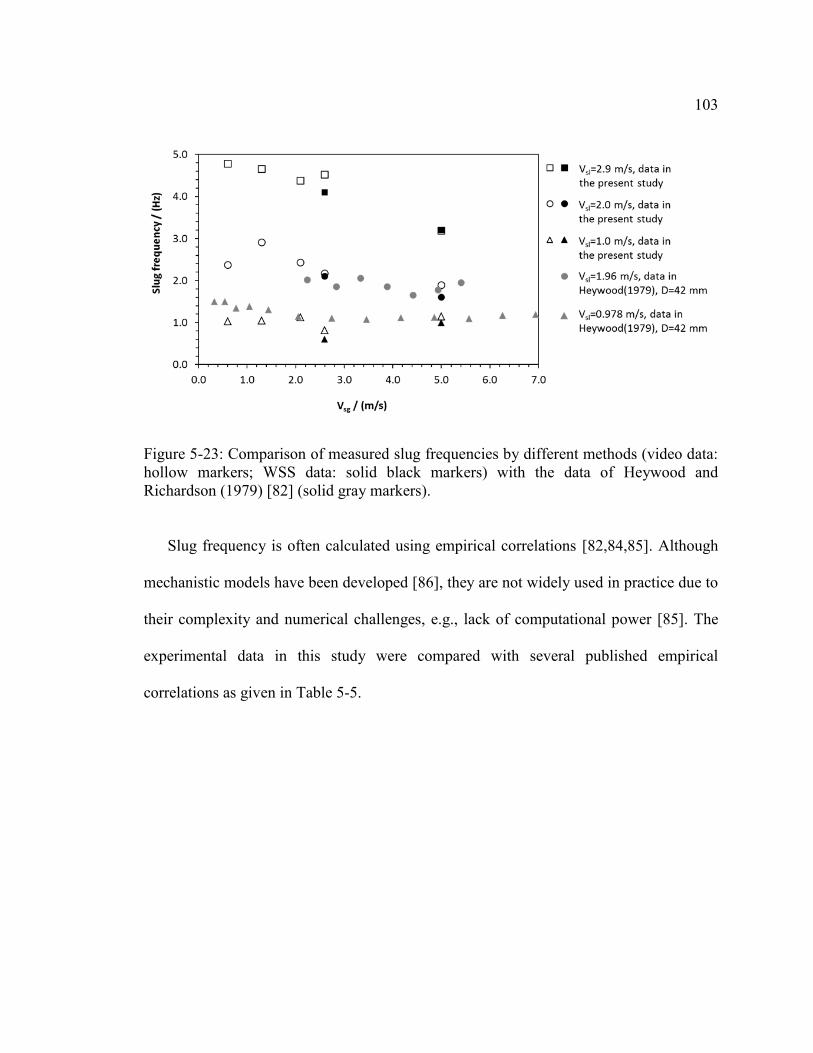
103
Figure 5-23: Comparison of measured slug frequencies by different methods (video data: hollow markers; WSS data: solid black markers) with the data of Heywood and Richardson (1979) [82] (solid gray markers).
Slug frequency is often calculated using empirical correlations [82,84,85]. Although
mechanistic models have been developed [86], they are not widely used in practice due to
their complexity and numerical challenges, e.g., lack of computational power [85]. The
experimental data in this study were compared with several published empirical
correlations as given in Table 5-5.
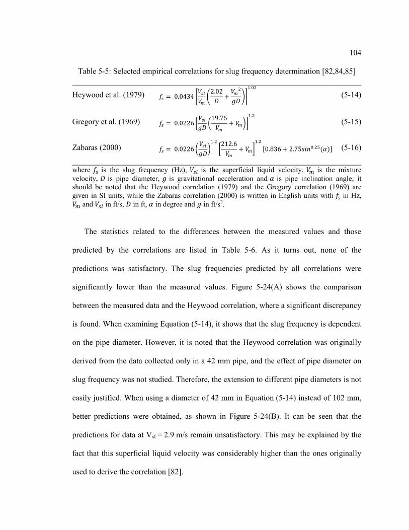
104
Table 5-5: Selected empirical correlations for slug frequency determination [82,84,85]
Heywood et al. (1979) 𝑓𝑠 = 0.0434 [𝑉𝑠𝑙
𝑉𝑚
(2.02
𝐷+
𝑉𝑚2
𝑔𝐷)]
1.02
(5-14)
Gregory et al. (1969) 𝑓𝑠 = 0.0226 [𝑉𝑠𝑙
𝑔𝐷(
19.75
𝑉𝑚
+ 𝑉𝑚)]1.2
(5-15)
Zabaras (2000) 𝑓𝑠 = 0.0226 (𝑉𝑠𝑙
𝑔𝐷)
1.2
[212.6
𝑉𝑚
+ 𝑉𝑚]1.2
[0.836 + 2.75𝑠𝑖𝑛0.25(𝛼)] (5-16)
where 𝑓𝑠 is the slug frequency (Hz), 𝑉𝑠𝑙 is the superficial liquid velocity, 𝑉𝑚 is the mixture velocity, 𝐷 is pipe diameter, 𝑔 is gravitational acceleration and 𝛼 is pipe inclination angle; it should be noted that the Heywood correlation (1979) and the Gregory correlation (1969) are given in SI units, while the Zabaras correlation (2000) is written in English units with 𝑓𝑠 in Hz, 𝑉𝑚 and 𝑉𝑠𝑙 in ft/s, 𝐷 in ft, 𝛼 in degree and 𝑔 in ft/s2.
The statistics related to the differences between the measured values and those
predicted by the correlations are listed in Table 5-6. As it turns out, none of the
predictions was satisfactory. The slug frequencies predicted by all correlations were
significantly lower than the measured values. Figure 5-24(A) shows the comparison
between the measured data and the Heywood correlation, where a significant discrepancy
is found. When examining Equation (5-14), it shows that the slug frequency is dependent
on the pipe diameter. However, it is noted that the Heywood correlation was originally
derived from the data collected only in a 42 mm pipe, and the effect of pipe diameter on
slug frequency was not studied. Therefore, the extension to different pipe diameters is not
easily justified. When using a diameter of 42 mm in Equation (5-14) instead of 102 mm,
better predictions were obtained, as shown in Figure 5-24(B). It can be seen that the
predictions for data at Vsl = 2.9 m/s remain unsatisfactory. This may be explained by the
fact that this superficial liquid velocity was considerably higher than the ones originally
used to derive the correlation [82].

105
Table 5-6: Error statistics for slug frequency: (predicted – measured)/measured,
for the data produced by using different empirical correlations
Correlations Heywood et al. (1979)
Gregory et al. (1969)
Zabaras (2000)
Average error (%) -59.3 -64.9 -70.7
Standard deviation (%) 12.0 9.2 7.7
Average absolute error (%) 59.3 64.9 70.7
Standard deviation of absolute error (%) 12.0 9.2 7.7
Overall, the results suggest that empirical correlations derived from a limited number
of data in a specific test setup may not be reliable when applying them to systems where
flow conditions (e.g., velocities, pipe diameters) are outside the original data set range. In
addition, all existing empirical correlations may suffer to some degree from laboratory
loop artefacts as the slug frequency in many laboratory facilities may be influenced by
factors such as the inlet geometry, upstream details (e.g., presence of a gas buffer) and
the length of the loop. Mechanistic approaches such as that given by, for example, the
Taitel and Dukler model [86] are therefore recommended for accurate slug frequency
predictions, even if these are much more complicated to implement [85].
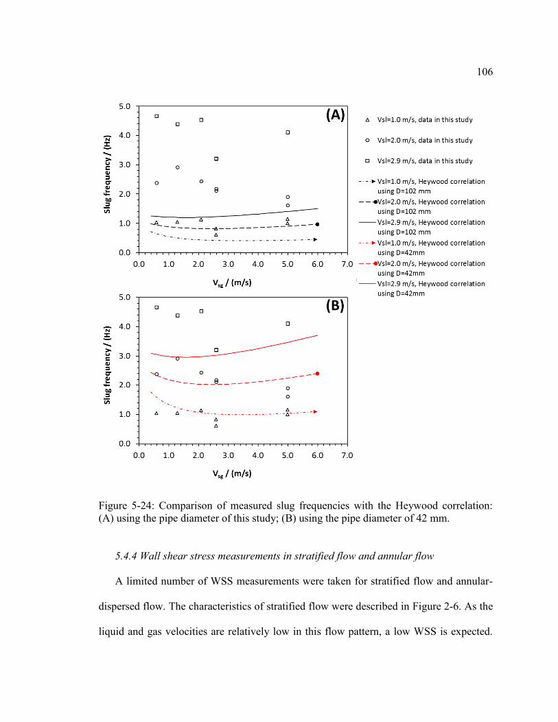
106
Figure 5-24: Comparison of measured slug frequencies with the Heywood correlation: (A) using the pipe diameter of this study; (B) using the pipe diameter of 42 mm.
5.4.4 Wall shear stress measurements in stratified flow and annular flow
A limited number of WSS measurements were taken for stratified flow and annular-
dispersed flow. The characteristics of stratified flow were described in Figure 2-6. As the
liquid and gas velocities are relatively low in this flow pattern, a low WSS is expected.
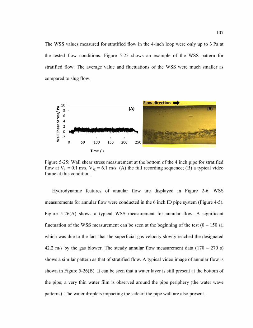
107
The WSS values measured for stratified flow in the 4-inch loop were only up to 3 Pa at
the tested flow conditions. Figure 5-25 shows an example of the WSS pattern for
stratified flow. The average value and fluctuations of the WSS were much smaller as
compared to slug flow.
Figure 5-25: Wall shear stress measurement at the bottom of the 4 inch pipe for stratified flow at Vsl = 0.1 m/s, Vsg = 6.1 m/s: (A) the full recording sequence; (B) a typical video frame at this condition.
Hydrodynamic features of annular flow are displayed in Figure 2-6. WSS
measurements for annular flow were conducted in the 6 inch ID pipe system (Figure 4-5).
Figure 5-26(A) shows a typical WSS measurement for annular flow. A significant
fluctuation of the WSS measurement can be seen at the beginning of the test (0 – 150 s),
which was due to the fact that the superficial gas velocity slowly reached the designated
42.2 m/s by the gas blower. The steady annular flow measurement data (170 – 270 s)
shows a similar pattern as that of stratified flow. A typical video image of annular flow is
shown in Figure 5-26(B). It can be seen that a water layer is still present at the bottom of
the pipe; a very thin water film is observed around the pipe periphery (the water wave
patterns). The water droplets impacting the side of the pipe wall are also present.
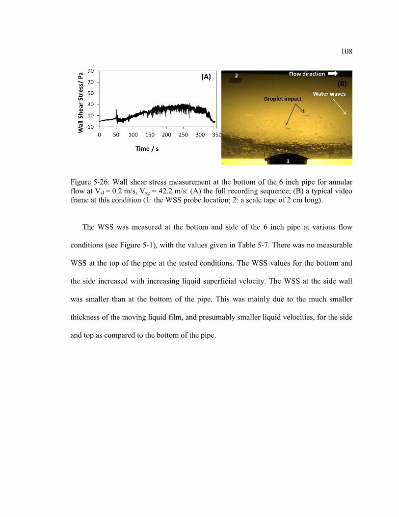
108
Figure 5-26: Wall shear stress measurement at the bottom of the 6 inch pipe for annular flow at Vsl = 0.2 m/s, Vsg = 42.2 m/s: (A) the full recording sequence; (B) a typical video frame at this condition (1: the WSS probe location; 2: a scale tape of 2 cm long).
The WSS was measured at the bottom and side of the 6 inch pipe at various flow
conditions (see Figure 5-1), with the values given in Table 5-7. There was no measurable
WSS at the top of the pipe at the tested conditions. The WSS values for the bottom and
the side increased with increasing liquid superficial velocity. The WSS at the side wall
was smaller than at the bottom of the pipe. This was mainly due to the much smaller
thickness of the moving liquid film, and presumably smaller liquid velocities, for the side
and top as compared to the bottom of the pipe.
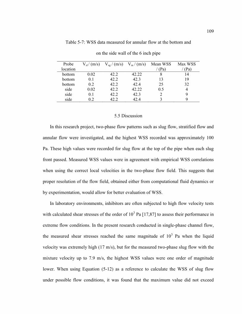
109
Table 5-7: WSS data measured for annular flow at the bottom and
on the side wall of the 6 inch pipe
Probe location
Vsl / (m/s) Vsg / (m/s) Vm / (m/s) Mean WSS / (Pa)
Max WSS / (Pa)
bottom 0.02 42.2 42.22 8 14 bottom 0.1 42.2 42.3 13 19 bottom 0.2 42.2 42.4 25 32
side 0.02 42.2 42.22 0.5 4 side 0.1 42.2 42.3 2 9 side 0.2 42.2 42.4 3 9
5.5 Discussion
In this research project, two-phase flow patterns such as slug flow, stratified flow and
annular flow were investigated, and the highest WSS recorded was approximately 100
Pa. These high values were recorded for slug flow at the top of the pipe when each slug
front passed. Measured WSS values were in agreement with empirical WSS correlations
when using the correct local velocities in the two-phase flow field. This suggests that
proper resolution of the flow field, obtained either from computational fluid dynamics or
by experimentation, would allow for better evaluation of WSS.
In laboratory environments, inhibitors are often subjected to high flow velocity tests
with calculated shear stresses of the order of 103 Pa [17,87] to assess their performance in
extreme flow conditions. In the present research conducted in single-phase channel flow,
the measured shear stresses reached the same magnitude of 103 Pa when the liquid
velocity was extremely high (17 m/s), but for the measured two-phase slug flow with the
mixture velocity up to 7.9 m/s, the highest WSS values were one order of magnitude
lower. When using Equation (5-12) as a reference to calculate the WSS of slug flow
under possible flow conditions, it was found that the maximum value did not exceed

110
1000 Pa with mixture velocities up to 30 m/s and gas densities up to 100 kg/m3 in a 4-
inch-ID pipe. This suggests that the maximum WSS in realistic multiphase pipe flow
under most extreme conditions would be of the order of 103 Pa.
Recalling the fact that the stresses required to remove inhibitor films and/or FeCO3
layers are at least 106 Pa in magnitude [9,11,19,22], there is a large gap between the
required stresses to remove these films/layers and flow shear stresses measured or
expected in practice. It may therefore be concluded that the high values of WSS found in
multiphase flow cannot lead to purely mechanical removal of inhibitor films and
protective corrosion product layers.
Although the floating element probe was used to successfully measure the WSS in the
multiphase flow, some possible shortcomings in the present research program have been
identified and are discussed below. The spatial and temporal resolutions of the WSS
probe do not allow measurement of very short-lived WSS values (fluctuations) occurring
over very small length scales.
The floating element on the WSS probe has a diameter of 6 mm, which still can be
much larger than the scale of some turbulent eddies. The smallest hydrodynamic scale in
turbulent flow can be estimated by the Kolmogorov length scale ( 𝜂 ), which is
approximately of the order of 10 - 100 µm in laboratory environments such as the one
used here [88,89]. Therefore, to accurately measure local WSS from small turbulent
eddies, a floating element with spatial dimensions of the order of 10-100 µm may be
necessary. The time scales associated with the smallest of eddies are of the order of ms,
or even less, putting an additional requirement on the temporal resolution of the

111
measurements. On the other hand, the energy levels associated with the smallest eddies
are also very low and it is not expected that they can contribute to a significant increase
of the time/space averaged WSS, such as the one measured here.
Using the highest recording rate of 1000 Hz, the WSS probe provided reasonable
measurements when it comes to the large time scale transients found in multiphase flows,
such as, for example, during slugging. For instance, the slug frequency was only a few
hertz, and any WSS fluctuations due to the passage of slugs would have been accurately
recorded by the floating element probe.
While a number of different multiphase flow patterns were investigated in the present
work, it is believed that some specific flow conditions found in the field, involving a
discrete phase, were not covered by our testing. A good example is liquid droplet
impingement found in annular-mist flow which may lead to much larger fluctuations of
the WSS magnitude than recorded in the present study. Annular-mist flow with entrained
liquid droplets, traveling at the gas velocity, can lead to high energy wall impacts
particularly at locations of disturbed flow, such as bends, valves, tees, weld beads, etc.
Very high local WSS and normal stresses could be found at impact locations [90],
particularly when there is little “cushioning” by an existing liquid film. Laboratory tests
have shown droplets having sizes of the order of 100 μm [91], which would produce very
short lived, high energy fluctuations at impact time. Therefore, a WSS probe would be
required to have both high temporal and spatial resolutions in order to capture this
behavior. This is an area that needs to be covered by future research.
112
5.6 Summary
The summary of the key findings of the research described in this chapter is given
below:
The floating element method was successful in directly measuring wall shear
stress in the studied multiphase flow, which provides valuable data for
mechanistic modeling.
The highest wall shear stress in horizontal slug flow occurred on the top section of
the pipe when the slug front passed. The higher wall shear stress as compared to
the bottom was because of the higher local in situ liquid flow velocity. The
maximum shear stress value was about 2 to 4 times higher than the calculated
mean shear stress of the slug body using mixture velocity, which can serve as a
guideline for improving slug flow modeling. When the correct local velocity is
used, the calculations of the wall shear stress were in good agreement with the
measured values.
In multiphase flow, studied here at ambient conditions, the maximum wall shear
stress was of an order of 102 Pa, obtained in slug flow. Using a model it was
estimated that the highest practical wall shear stress that could be expected in the
field is of the order of 103 Pa.
This suggests that purely mechanical removal of inhibitor films or FeCO3 layers
solely by wall shear stress, typically seen in multiphase flow pipelines, is very
unlikely. As failures of these protective films/layers in multiphase flow are

113
observed in laboratory and field studies, other factors associated with multiphase
flow must be considered.
114
Chapter 6: Mechanical Effects of Flow on CO2 Corrosion Inhibition
6.1 Introduction
In the previous chapter, it is found that the measured WSS in typical multiphase flow
pipelines is several orders of magnitude lower than the required stresses to remove
inhibitor films or corrosion product layers from the steel surface. Purely mechanical
removal of these films/layers solely by WSS is therefore very unlikely. In this chapter,
the hypothesis that surface geometric irregularity can locally lead to high instantaneous
hydrodynamic stresses and interfere with the corrosion inhibitor adsorption/desorption
processes is examined. In addition, other factors that may affect corrosion inhibitor films,
e.g., oxygen ingress, are studied. Last but not least, the mechanisms of how flow
mechanically affects the corrosion inhibitors are discussed.
6.2 Experimental
6.2.1 Flow system for corrosion tests
Experiments were performed in the earlier described thin channel flow cell system
(Figure 4-2). Due to the high flow velocity in the thin channel, a high wall shear stress
environment was expected. The flow generated by this system is considered to be the
most turbulent that can be simulated in our laboratory and was used to investigate the
mechanical integrity of TOFA/DETA imidazolinium inhibitor films in the presence of
high mechanical stresses.
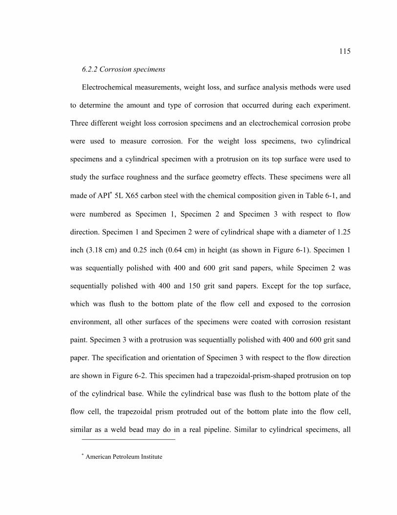
115
6.2.2 Corrosion specimens
Electrochemical measurements, weight loss, and surface analysis methods were used
to determine the amount and type of corrosion that occurred during each experiment.
Three different weight loss corrosion specimens and an electrochemical corrosion probe
were used to measure corrosion. For the weight loss specimens, two cylindrical
specimens and a cylindrical specimen with a protrusion on its top surface were used to
study the surface roughness and the surface geometry effects. These specimens were all
made of API 5L X65 carbon steel with the chemical composition given in Table 6-1, and
were numbered as Specimen 1, Specimen 2 and Specimen 3 with respect to flow
direction. Specimen 1 and Specimen 2 were of cylindrical shape with a diameter of 1.25
inch (3.18 cm) and 0.25 inch (0.64 cm) in height (as shown in Figure 6-1). Specimen 1
was sequentially polished with 400 and 600 grit sand papers, while Specimen 2 was
sequentially polished with 400 and 150 grit sand papers. Except for the top surface,
which was flush to the bottom plate of the flow cell and exposed to the corrosion
environment, all other surfaces of the specimens were coated with corrosion resistant
paint. Specimen 3 with a protrusion was sequentially polished with 400 and 600 grit sand
paper. The specification and orientation of Specimen 3 with respect to the flow direction
are shown in Figure 6-2. This specimen had a trapezoidal-prism-shaped protrusion on top
of the cylindrical base. While the cylindrical base was flush to the bottom plate of the
flow cell, the trapezoidal prism protruded out of the bottom plate into the flow cell,
similar as a weld bead may do in a real pipeline. Similar to cylindrical specimens, all
American Petroleum Institute

116
other surfaces of the specimen below the bottom plate of the flow cell were coated with
corrosion resistant paint. The top surface of the protrusion specimen exposed to the
corrosion environment was defined by 5 individual regions as shown in Figure 6-2 for
surface analysis.
Table 6-1: Chemical analysis [wt.%] of API 5L X65 carbon steel
C Mn Nb P S Ti V Fe 0.05 1.51 0.03 0.004 0.001 0.01 0.04 balance
Figure 6-1: Specification and flow orientation for flat weight loss specimens. Left: side view; right: top view.
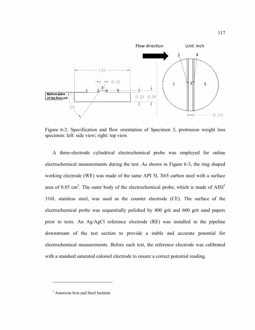
117
Figure 6-2: Specification and flow orientation of Specimen 3, protrusion weight loss specimen: left: side view; right: top view.
A three-electrode cylindrical electrochemical probe was employed for online
electrochemical measurements during the test. As shown in Figure 6-3, the ring shaped
working electrode (WE) was made of the same API 5L X65 carbon steel with a surface
area of 0.85 cm2. The outer body of the electrochemical probe, which is made of AISI†
316L stainless steel, was used as the counter electrode (CE). The surface of the
electrochemical probe was sequentially polished by 400 grit and 600 grit sand papers
prior to tests. An Ag/AgCl reference electrode (RE) was installed in the pipeline
downstream of the test section to provide a stable and accurate potential for
electrochemical measurements. Before each test, the reference electrode was calibrated
with a standard saturated calomel electrode to ensure a correct potential reading.
† American Iron and Steel Institute

118
Figure 6-3: Configuration of the electrochemical probe.
The three weight loss specimens and the electrochemical probe were flush-mounted
to the bottom plate in the TCFC test section in a sequence as shown in Figure 6-4. All
weight loss specimens were fixed in position by using a mechanical specimen holder
underneath (as shown in Figure 6-4). The protrusion specimen (Specimen 3) was placed
furthest downstream (port 4) to minimize the flow disturbance to other specimens.

119
Figure 6-4: Location arrangement of the specimens in the TCFC.
6.2.3 Experimental procedures
The test matrix for this work is shown in Table 6-2. The tests were maintained at
25oC, 0.97 bar CO2 partial pressure and a pH value of 5.0 to achieve a low FeCO3
saturation value (S(FeCO3) << 1) [6]. Accordingly, no FeCO3 was expected or observed on
the specimen surfaces in any of the following experiments, which was confirmed by SEM
analysis. The inhibitor used was TOFA/DETA imidazolinium (K1 ).
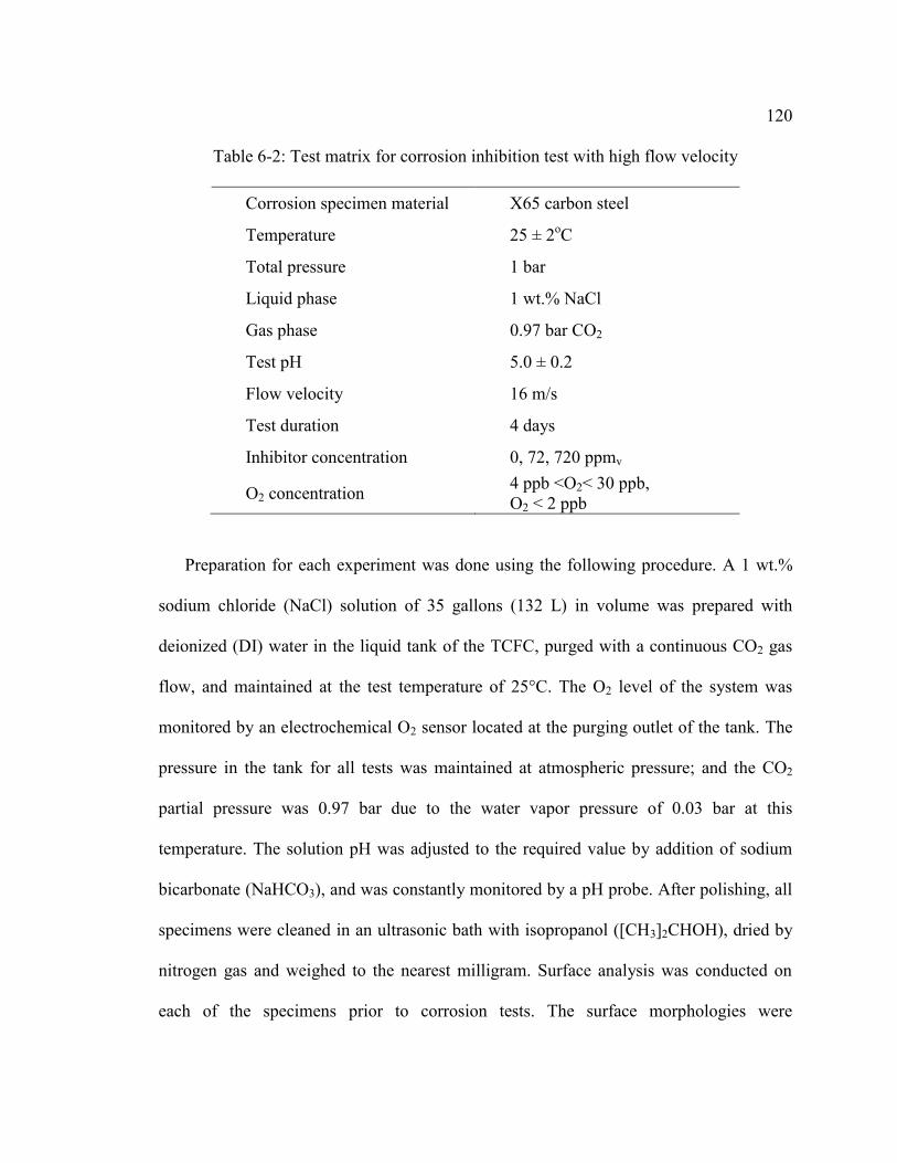
120
Table 6-2: Test matrix for corrosion inhibition test with high flow velocity
Corrosion specimen material X65 carbon steel
Temperature 25 ± 2oC
Total pressure 1 bar
Liquid phase 1 wt.% NaCl
Gas phase 0.97 bar CO2
Test pH 5.0 ± 0.2
Flow velocity 16 m/s
Test duration 4 days
Inhibitor concentration 0, 72, 720 ppmv
O2 concentration 4 ppb <O2< 30 ppb, O2 < 2 ppb
Preparation for each experiment was done using the following procedure. A 1 wt.%
sodium chloride (NaCl) solution of 35 gallons (132 L) in volume was prepared with
deionized (DI) water in the liquid tank of the TCFC, purged with a continuous CO2 gas
flow, and maintained at the test temperature of 25°C. The O2 level of the system was
monitored by an electrochemical O2 sensor located at the purging outlet of the tank. The
pressure in the tank for all tests was maintained at atmospheric pressure; and the CO2
partial pressure was 0.97 bar due to the water vapor pressure of 0.03 bar at this
temperature. The solution pH was adjusted to the required value by addition of sodium
bicarbonate (NaHCO3), and was constantly monitored by a pH probe. After polishing, all
specimens were cleaned in an ultrasonic bath with isopropanol ([CH3]2CHOH), dried by
nitrogen gas and weighed to the nearest milligram. Surface analysis was conducted on
each of the specimens prior to corrosion tests. The surface morphologies were

121
characterized by scanning electron microscopy (SEM) and profilometry. After surface
analysis, all specimens were rinsed with isopropanol and flush-mounted to the bottom
plate of the TCFC test section. The test section was then deaerated with dry CO2 gas.
Finally, the prepared test solution in the liquid tank was diverted to the test section at the
designated flow velocity, pH, O2 concentration and temperature.
During each experiment, a potentiostat connected with the electrochemical corrosion
probe was used for performing electrochemical measurements. The open-circuit potential
(OCP) was continuously monitored and linear polarization resistance (LPR)
measurements were conducted systematically to provide in situ corrosion rate
measurements. The potential polarization range was ± 5 mV versus OCP with a scanning
rate of 0.1 mV/s. The solution resistance was measured with electrochemical impedance
spectroscopy (EIS) to ensure satisfactory solution conductivity. Deaerated corrosion
inhibitor was added to the system typically 10 – 12 hours after the beginning of the
experiment when the corrosion rate was stable. Each experiment typically lasted another
4 days after the addition of inhibitor. In this work, a surfactant-type inhibitor,
TOFA/DETA imidazolinium salt, was used. The molecular structure of this inhibitor is
well understood, as depicted in Figure 2-5. A typical inhibitor concentration of 72 ppmv
was used in the tests, which exceeded the reported CMC value for this inhibitor [22,92]
and should effectively mitigate the corrosion at the tested temperature and pH [93,94].
After the corrosion test, all weight loss specimens were carefully taken out of the
TCFC, immediately immersed into deaerated deionized water to remove soluble salts and
impurities on the specimen surface. Sequentially, the specimens were cleaned in an
122
ultrasonic bath with isopropanol, dried by nitrogen gas, weighed to the nearest milligram,
and stored in a vacuum desiccator for further after-test surface analyses.
6.3 Experimental Results
The focus of this work is to determine how mechanical stresses produced by turbulent
flow affect corrosion inhibitor films. Wall shear stress (WSS) is one of the most
important forms of hydrodynamic stresses to characterize flow conditions. In this study,
the flow velocity in the TCFC test section was 16 m/s. The average WSS at the bottom
plate of the TCFC was corroborated by measurements using a floating element WSS
sensor (see Figure 5-2) to be approximately 700 - 800 Pa when the flow velocity was
16 m/s. But a special protrusion specimen was also used in this research, which was
expected to significantly change the local hydrodynamic conditions, lead to a higher local
WSS, and affect inhibitor films on the metal surface.
6.3.1 Corrosion tests without inhibitor
A blank test without addition of corrosion inhibitor was conducted, and the corrosion
rates were measured by weight loss and LPR. The details of corrosion rate calculation by
these two methods are described in Appendix 3. The weight losses from all three
corrosion specimens were measured and the average corrosion rate was calculated to be
5.7 ± 0.4 mm/yr.

123
The corrosion rate was also determined by the LPR technique, which measures the
polarization resistance of the working electrode and calculates the corrosion current
(𝐼𝑐𝑜𝑟𝑟) by the Stern-Geary equation [57]:
𝐼𝑐𝑜𝑟𝑟 =𝐵
𝑅𝑝 (6-1)
where Rp is the polarization resistance (ohm) and B is the proportionality constant, or B
value (V). For corrosion of steel (iron), the calculated corrosion current is related to the
corrosion rate, as given by:
𝐶𝑅 = 1.16 ∙𝐼𝑐𝑜𝑟𝑟
𝑆 (6-2)
where 𝐶𝑅 is the corrosion rate (mm/yr); 𝐼𝑐𝑜𝑟𝑟 is the corrosion current (A); and 𝑆 is the
surface area of the electrode (m2). The overall formula of corrosion rate calculation can
be written as:
𝐶𝑅 =1.16𝐵
𝑆𝑅𝑝 (6-3)
It should be noted that the B value is required to calculate the corrosion rate for the LPR
technique, and quite often it is not known a priori.
The measured average corrosion rate from weight loss and polarization resistance
from LPR were substituted in Equation (6-3) to determine the B value for the corrosion
experiments in this study. Since the average corrosion rate from weight loss measurement
was 5.7 mm/yr, the surface area of the electrode was 0.85×10⁻⁴ m2, and the time-averaged
polarization resistance from the LPR measurements was calculated to be 156 ohms, an
averaged B value of 65 mV was obtained. This B value was used throughout the entire
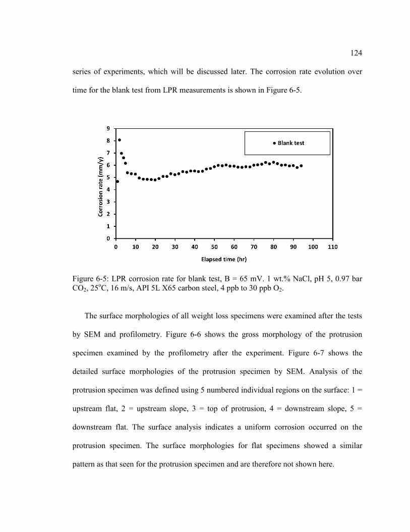
124
series of experiments, which will be discussed later. The corrosion rate evolution over
time for the blank test from LPR measurements is shown in Figure 6-5.
Figure 6-5: LPR corrosion rate for blank test, B = 65 mV. 1 wt.% NaCl, pH 5, 0.97 bar CO2, 25oC, 16 m/s, API 5L X65 carbon steel, 4 ppb to 30 ppb O2.
The surface morphologies of all weight loss specimens were examined after the tests
by SEM and profilometry. Figure 6-6 shows the gross morphology of the protrusion
specimen examined by the profilometry after the experiment. Figure 6-7 shows the
detailed surface morphologies of the protrusion specimen by SEM. Analysis of the
protrusion specimen was defined using 5 numbered individual regions on the surface: 1 =
upstream flat, 2 = upstream slope, 3 = top of protrusion, 4 = downstream slope, 5 =
downstream flat. The surface analysis indicates a uniform corrosion occurred on the
protrusion specimen. The surface morphologies for flat specimens showed a similar
pattern as that seen for the protrusion specimen and are therefore not shown here.
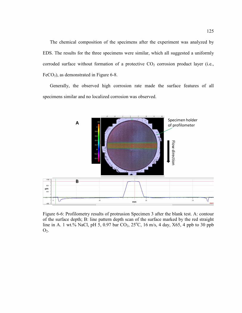
125
The chemical composition of the specimens after the experiment was analyzed by
EDS. The results for the three specimens were similar, which all suggested a uniformly
corroded surface without formation of a protective CO2 corrosion product layer (i.e.,
FeCO3), as demonstrated in Figure 6-8.
Generally, the observed high corrosion rate made the surface features of all
specimens similar and no localized corrosion was observed.
Figure 6-6: Profilometry results of protrusion Specimen 3 after the blank test. A: contour of the surface depth; B: line pattern depth scan of the surface marked by the red straight line in A. 1 wt.% NaCl, pH 5, 0.97 bar CO2, 25oC, 16 m/s, 4 day, X65, 4 ppb to 30 ppb O2.
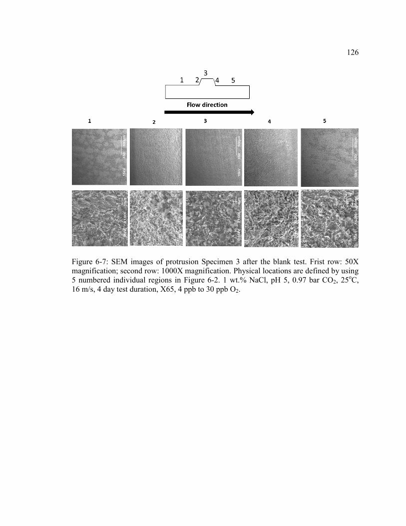
126
Figure 6-7: SEM images of protrusion Specimen 3 after the blank test. Frist row: 50X magnification; second row: 1000X magnification. Physical locations are defined by using 5 numbered individual regions in Figure 6-2. 1 wt.% NaCl, pH 5, 0.97 bar CO2, 25oC, 16 m/s, 4 day test duration, X65, 4 ppb to 30 ppb O2.
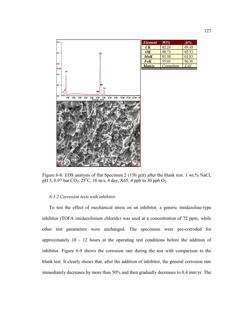
127
Figure 6-8: EDS analysis of flat Specimen 2 (150 grit) after the blank test. 1 wt.% NaCl, pH 5, 0.97 bar CO2, 25oC, 16 m/s, 4 day, X65, 4 ppb to 30 ppb O2.
6.3.2 Corrosion tests with inhibitor
To test the effect of mechanical stress on an inhibitor, a generic imidazoline-type
inhibitor (TOFA imidazolinium chloride) was used at a concentration of 72 ppmv while
other test parameters were unchanged. The specimens were pre-corroded for
approximately 10 - 12 hours at the operating test conditions before the addition of
inhibitor. Figure 6-9 shows the corrosion rate during the test with comparison to the
blank test. It clearly shows that, after the addition of inhibitor, the general corrosion rate
immediately decreases by more than 50% and then gradually decreases to 0.4 mm/yr. The
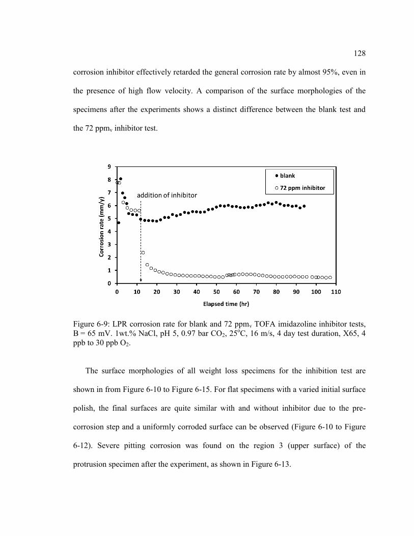
128
corrosion inhibitor effectively retarded the general corrosion rate by almost 95%, even in
the presence of high flow velocity. A comparison of the surface morphologies of the
specimens after the experiments shows a distinct difference between the blank test and
the 72 ppmv inhibitor test.
Figure 6-9: LPR corrosion rate for blank and 72 ppmv TOFA imidazoline inhibitor tests, B = 65 mV. 1wt.% NaCl, pH 5, 0.97 bar CO2, 25oC, 16 m/s, 4 day test duration, X65, 4 ppb to 30 ppb O2.
The surface morphologies of all weight loss specimens for the inhibition test are
shown in from Figure 6-10 to Figure 6-15. For flat specimens with a varied initial surface
polish, the final surfaces are quite similar with and without inhibitor due to the pre-
corrosion step and a uniformly corroded surface can be observed (Figure 6-10 to Figure
6-12). Severe pitting corrosion was found on the region 3 (upper surface) of the
protrusion specimen after the experiment, as shown in Figure 6-13.

129
Figure 6-10: SEM images of flat Specimen 1 (600 grit finish) and Specimen 2 (150 grit finish) at 1000X magnification. 1 wt.% NaCl, pH 5, 0.97 bar CO2, 25oC, 72 ppmv inhibitor, 16 m/s, 4 day test duration, X65, 4 ppb to 30 ppb O2: A. Specimen 1 before test; B. Specimen 1 after test; C. Specimen 2 before test; D. Specimen 2 after test.

130
Figure 6-11: Profilometry results of flat Specimen 1 (600 grit finish) after the test. A: contour of the surface depth; B: line pattern depth scan of the surface marked by the red straight line in A.
Figure 6-12: Profilometry results of flat Specimen 2 (150 grit finish) after the test. A: contour of the surface depth; B: line pattern depth scan of the surface marked by the red straight line in A.
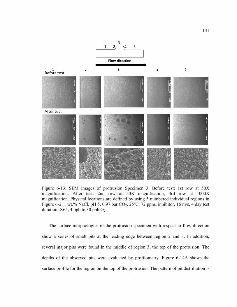
131
Figure 6-13: SEM images of protrusion Specimen 3. Before test: 1st row at 50X magnification. After test: 2nd row at 50X magnification; 3rd row at 1000X magnification. Physical locations are defined by using 5 numbered individual regions in Figure 6-2. 1 wt.% NaCl, pH 5, 0.97 bar CO2, 25oC, 72 ppmv inhibitor, 16 m/s, 4 day test duration, X65, 4 ppb to 30 ppb O2.
The surface morphologies of the protrusion specimen with respect to flow direction
show a series of small pits at the leading edge between region 2 and 3. In addition,
several major pits were found in the middle of region 3, the top of the protrusion. The
depths of the observed pits were evaluated by profilometry. Figure 6-14A shows the
surface profile for the region on the top of the protrusion. The pattern of pit distribution is
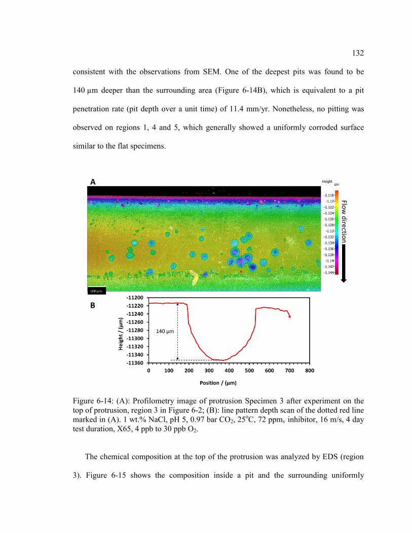
132
consistent with the observations from SEM. One of the deepest pits was found to be
140 µm deeper than the surrounding area (Figure 6-14B), which is equivalent to a pit
penetration rate (pit depth over a unit time) of 11.4 mm/yr. Nonetheless, no pitting was
observed on regions 1, 4 and 5, which generally showed a uniformly corroded surface
similar to the flat specimens.
Figure 6-14: (A): Profilometry image of protrusion Specimen 3 after experiment on the top of protrusion, region 3 in Figure 6-2; (B): line pattern depth scan of the dotted red line marked in (A). 1 wt.% NaCl, pH 5, 0.97 bar CO2, 25oC, 72 ppmv inhibitor, 16 m/s, 4 day test duration, X65, 4 ppb to 30 ppb O2.
The chemical composition at the top of the protrusion was analyzed by EDS (region
3). Figure 6-15 shows the composition inside a pit and the surrounding uniformly
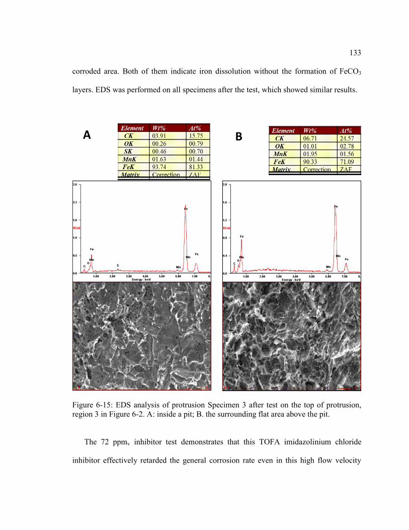
133
corroded area. Both of them indicate iron dissolution without the formation of FeCO3
layers. EDS was performed on all specimens after the test, which showed similar results.
Figure 6-15: EDS analysis of protrusion Specimen 3 after test on the top of protrusion, region 3 in Figure 6-2. A: inside a pit; B. the surrounding flat area above the pit.
The 72 ppmv inhibitor test demonstrates that this TOFA imidazolinium chloride
inhibitor effectively retarded the general corrosion rate even in this high flow velocity
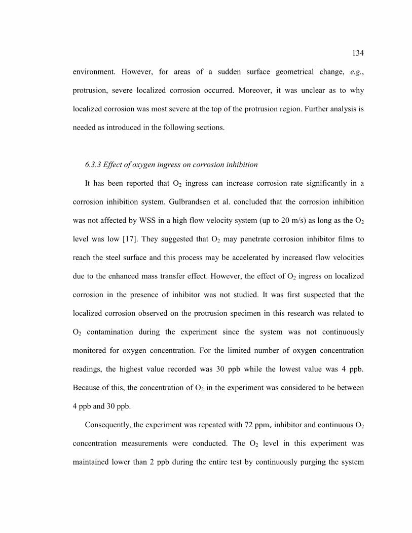
134
environment. However, for areas of a sudden surface geometrical change, e.g.,
protrusion, severe localized corrosion occurred. Moreover, it was unclear as to why
localized corrosion was most severe at the top of the protrusion region. Further analysis is
needed as introduced in the following sections.
6.3.3 Effect of oxygen ingress on corrosion inhibition
It has been reported that O2 ingress can increase corrosion rate significantly in a
corrosion inhibition system. Gulbrandsen et al. concluded that the corrosion inhibition
was not affected by WSS in a high flow velocity system (up to 20 m/s) as long as the O2
level was low [17]. They suggested that O2 may penetrate corrosion inhibitor films to
reach the steel surface and this process may be accelerated by increased flow velocities
due to the enhanced mass transfer effect. However, the effect of O2 ingress on localized
corrosion in the presence of inhibitor was not studied. It was first suspected that the
localized corrosion observed on the protrusion specimen in this research was related to
O2 contamination during the experiment since the system was not continuously
monitored for oxygen concentration. For the limited number of oxygen concentration
readings, the highest value recorded was 30 ppb while the lowest value was 4 ppb.
Because of this, the concentration of O2 in the experiment was considered to be between
4 ppb and 30 ppb.
Consequently, the experiment was repeated with 72 ppmv inhibitor and continuous O2
concentration measurements were conducted. The O2 level in this experiment was
maintained lower than 2 ppb during the entire test by continuously purging the system
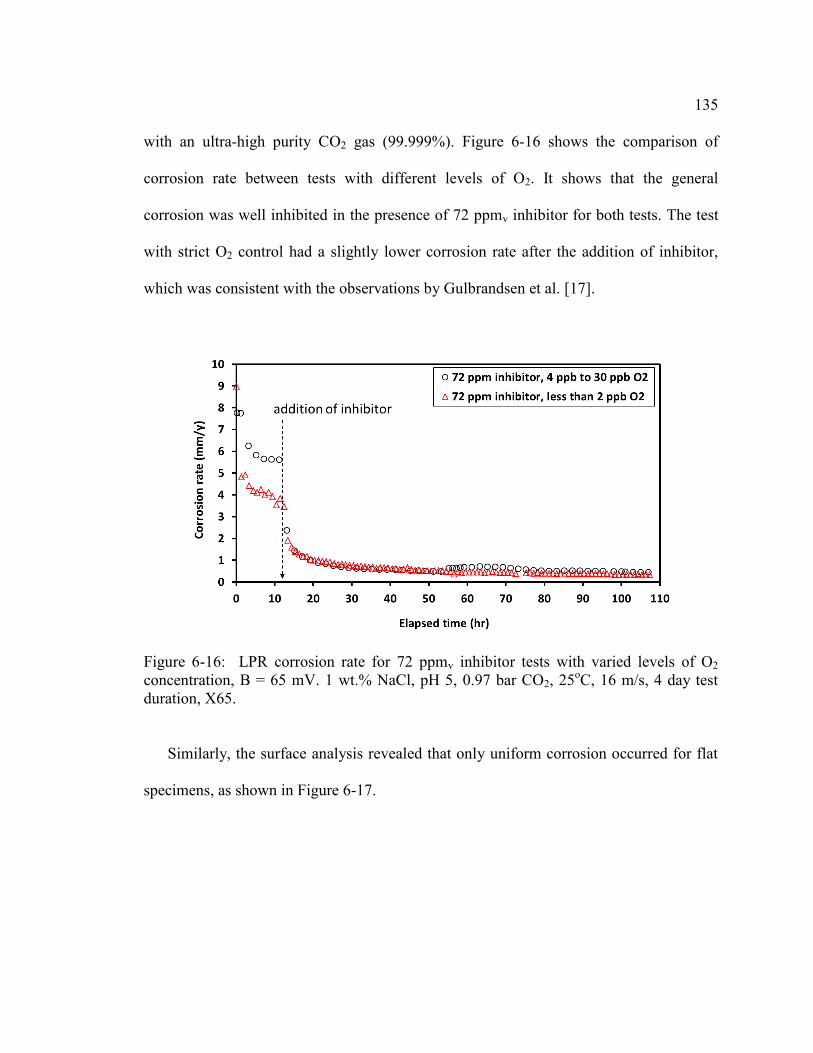
135
with an ultra-high purity CO2 gas (99.999%). Figure 6-16 shows the comparison of
corrosion rate between tests with different levels of O2. It shows that the general
corrosion was well inhibited in the presence of 72 ppmv inhibitor for both tests. The test
with strict O2 control had a slightly lower corrosion rate after the addition of inhibitor,
which was consistent with the observations by Gulbrandsen et al. [17].
Figure 6-16: LPR corrosion rate for 72 ppmv inhibitor tests with varied levels of O2 concentration, B = 65 mV. 1 wt.% NaCl, pH 5, 0.97 bar CO2, 25oC, 16 m/s, 4 day test duration, X65.
Similarly, the surface analysis revealed that only uniform corrosion occurred for flat
specimens, as shown in Figure 6-17.

136
Figure 6-17: SEM images of flat Specimen 1 (600 grit finish) and Specimen 2 (150 grit finish) at 1000X magnification. 1 wt.% NaCl, pH 5, 0.97 bar CO2, 25oC, 72 ppmv inhibitor, 16 m/s, 4 day test duration, X65, O2 < 2 ppb: A. Specimen 1 before test; B. Specimen 1 after test; C. Specimen 2 before test; D. Specimen 2 after test.
The surface morphology of the protrusion specimen before and after this experiment
is shown in Figure 6-18. Once again, pitting corrosion was found on the upstream slope
and top of the protrusion regions. Figure 6-19A shows the surface depth profile at the top
of the protrusion region obtained by profilometry. One of the deepest pits was found to be
154 µm below the surrounding area, which is equivalent to a pit penetration rate (PR) of
12.5 mm/yr.
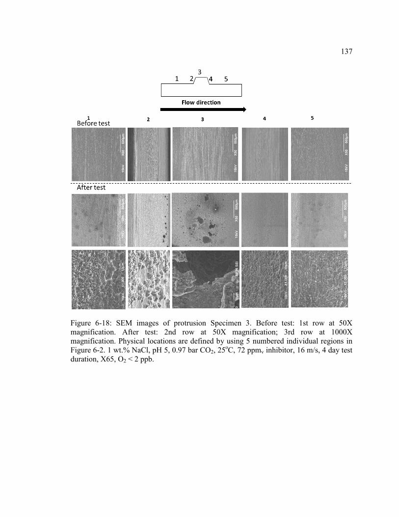
137
Figure 6-18: SEM images of protrusion Specimen 3. Before test: 1st row at 50X magnification. After test: 2nd row at 50X magnification; 3rd row at 1000X magnification. Physical locations are defined by using 5 numbered individual regions in Figure 6-2. 1 wt.% NaCl, pH 5, 0.97 bar CO2, 25oC, 72 ppmv inhibitor, 16 m/s, 4 day test duration, X65, O2 < 2 ppb.

138
Figure 6-19: (A): Profilometry image of protrusion Specimen 3 after experiment on top of protrusion, region 3 in Figure 6-2; (B): line pattern depth scan marked by the dotted red line in (A). 1 wt.% NaCl, pH 5, 0.97 bar CO2, 25oC, 72 ppmv inhibitor, 16 m/s, 4 day test duration, X65, O2 < 2 ppb.
The chemical composition of all specimens before and after the test was analyzed by
EDS, as shown in Figure 6-20, Figure 6-21 and Figure 6-22. In the low O2 environment,
all specimens showed similar results in that the steel surface was corroded with no FeCO3
layer formation.
139
Figure 6-20: EDS analysis of flat Specimen 1 (600 grit finish). A: before experiment; B. after experiment. 1 wt.% NaCl, pH 5, 0.97 bar CO2, 25oC, 72 ppmv inhibitor, 16 m/s, 4 day test duration, X65, O2 < 2 ppb.

140
Figure 6-21: EDS analysis of flat Specimen 2 (150 grit finish). A: before experiment; B. after experiment. 1 wt.% NaCl, pH 5, 0.97 bar CO2, 25oC, 72 ppmv inhibitor, 16 m/s, 4 day test duration, X65, O2 < 2 ppb.
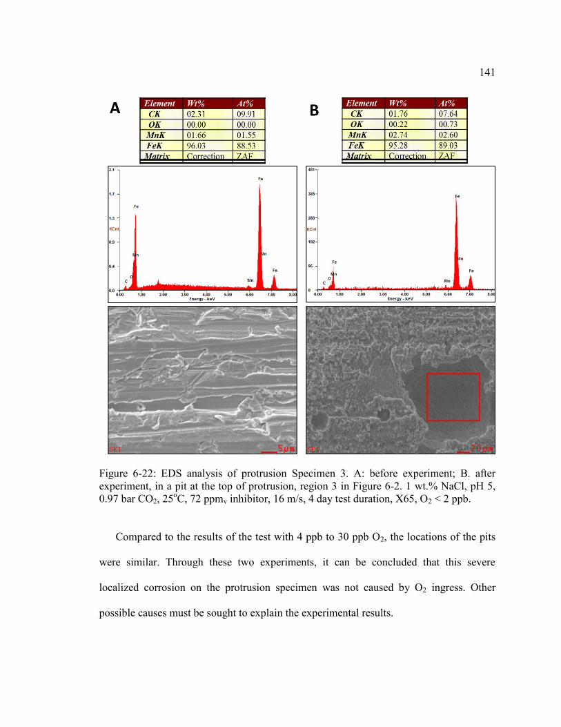
141
Figure 6-22: EDS analysis of protrusion Specimen 3. A: before experiment; B. after experiment, in a pit at the top of protrusion, region 3 in Figure 6-2. 1 wt.% NaCl, pH 5, 0.97 bar CO2, 25oC, 72 ppmv inhibitor, 16 m/s, 4 day test duration, X65, O2 < 2 ppb.
Compared to the results of the test with 4 ppb to 30 ppb O2, the locations of the pits
were similar. Through these two experiments, it can be concluded that this severe
localized corrosion on the protrusion specimen was not caused by O2 ingress. Other
possible causes must be sought to explain the experimental results.
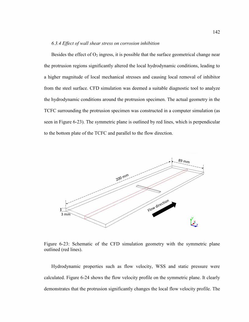
142
6.3.4 Effect of wall shear stress on corrosion inhibition
Besides the effect of O2 ingress, it is possible that the surface geometrical change near
the protrusion regions significantly altered the local hydrodynamic conditions, leading to
a higher magnitude of local mechanical stresses and causing local removal of inhibitor
from the steel surface. CFD simulation was deemed a suitable diagnostic tool to analyze
the hydrodynamic conditions around the protrusion specimen. The actual geometry in the
TCFC surrounding the protrusion specimen was constructed in a computer simulation (as
seen in Figure 6-23). The symmetric plane is outlined by red lines, which is perpendicular
to the bottom plate of the TCFC and parallel to the flow direction.
Figure 6-23: Schematic of the CFD simulation geometry with the symmetric plane outlined (red lines).
Hydrodynamic properties such as flow velocity, WSS and static pressure were
calculated. Figure 6-24 shows the flow velocity profile on the symmetric plane. It clearly
demonstrates that the protrusion significantly changes the local flow velocity profile. The
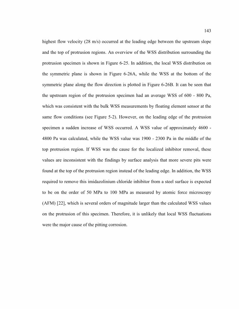
143
highest flow velocity (28 m/s) occurred at the leading edge between the upstream slope
and the top of protrusion regions. An overview of the WSS distribution surrounding the
protrusion specimen is shown in Figure 6-25. In addition, the local WSS distribution on
the symmetric plane is shown in Figure 6-26A, while the WSS at the bottom of the
symmetric plane along the flow direction is plotted in Figure 6-26B. It can be seen that
the upstream region of the protrusion specimen had an average WSS of 600 - 800 Pa,
which was consistent with the bulk WSS measurements by floating element sensor at the
same flow conditions (see Figure 5-2). However, on the leading edge of the protrusion
specimen a sudden increase of WSS occurred. A WSS value of approximately 4600 -
4800 Pa was calculated, while the WSS value was 1900 - 2300 Pa in the middle of the
top protrusion region. If WSS was the cause for the localized inhibitor removal, these
values are inconsistent with the findings by surface analysis that more severe pits were
found at the top of the protrusion region instead of the leading edge. In addition, the WSS
required to remove this imidazolinium chloride inhibitor from a steel surface is expected
to be on the order of 50 MPa to 100 MPa as measured by atomic force microscopy
(AFM) [22], which is several orders of magnitude larger than the calculated WSS values
on the protrusion of this specimen. Therefore, it is unlikely that local WSS fluctuations
were the major cause of the pitting corrosion.
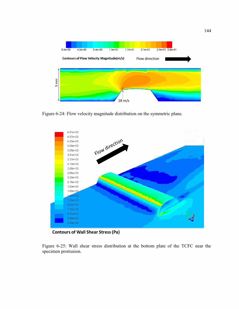
144
Figure 6-24: Flow velocity magnitude distribution on the symmetric plane.
Figure 6-25: Wall shear stress distribution at the bottom plate of the TCFC near the specimen protrusion.

145
Figure 6-26: Wall shear stress distribution: A. on the symmetric plane; B. on the bottom wall of the symmetric plane.
6.3.5 Effect of cavitation on corrosion inhibition
Because of the drastic increase of flow velocity at the leading edge of the protrusion,
the pressure at the same location was greatly reduced according to Bernoulli's principle
[95]. The pressure distribution on the symmetric plane along the flow direction is shown
in Figure 6-27A, which clearly illustrates such pressure fluctuations. From this graph, a
low pressure zone approximately -5.1 bar compared to the simulation inlet, is found at the

146
leading edge of the protrusion specimen. The pressure in the middle of the top protrusion
region then quickly recovers to -2.4 bar as compared to the simulation inlet. It should be
noted that the gauge pressure at the simulation outlet was set to be 0 bar as a reference
pressure.
Figure 6-27: Gauge pressure distribution: A. on the symmetric plane; B. on the bottom wall of the symmetric plane.
This unusual large pressure fluctuation at the leading edge may be the cause of the
pitting corrosion. During an additional experiment, pressure measurements at multiple
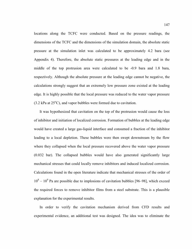
147
locations along the TCFC were conducted. Based on the pressure readings, the
dimensions of the TCFC and the dimensions of the simulation domain, the absolute static
pressure at the simulation inlet was calculated to be approximately 4.2 bara (see
Appendix 4). Therefore, the absolute static pressures at the leading edge and in the
middle of the top protrusion area were calculated to be -0.9 bara and 1.8 bara,
respectively. Although the absolute pressure at the leading edge cannot be negative, the
calculations strongly suggest that an extremely low pressure zone existed at the leading
edge. It is highly possible that the local pressure was reduced to the water vapor pressure
(3.2 kPa at 25oC), and vapor bubbles were formed due to cavitation.
It was hypothesized that cavitation on the top of the protrusion would cause the loss
of inhibitor and initiation of localized corrosion. Formation of bubbles at the leading edge
would have created a large gas-liquid interface and consumed a fraction of the inhibitor
leading to a local depletion. These bubbles were then swept downstream by the flow
where they collapsed when the local pressure recovered above the water vapor pressure
(0.032 bar). The collapsed bubbles would have also generated significantly large
mechanical stresses that could locally remove inhibitors and induced localized corrosion.
Calculations found in the open literature indicate that mechanical stresses of the order of
108 – 109 Pa are possible due to implosions of cavitation bubbles [96–98], which exceed
the required forces to remove inhibitor films from a steel substrate. This is a plausible
explanation for the experimental results.
In order to verify the cavitation mechanism derived from CFD results and
experimental evidence, an additional test was designed. The idea was to eliminate the
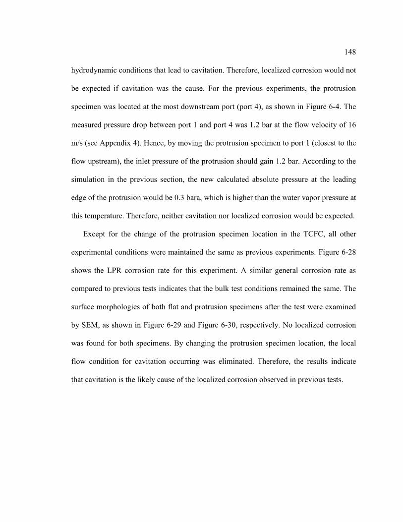
148
hydrodynamic conditions that lead to cavitation. Therefore, localized corrosion would not
be expected if cavitation was the cause. For the previous experiments, the protrusion
specimen was located at the most downstream port (port 4), as shown in Figure 6-4. The
measured pressure drop between port 1 and port 4 was 1.2 bar at the flow velocity of 16
m/s (see Appendix 4). Hence, by moving the protrusion specimen to port 1 (closest to the
flow upstream), the inlet pressure of the protrusion should gain 1.2 bar. According to the
simulation in the previous section, the new calculated absolute pressure at the leading
edge of the protrusion would be 0.3 bara, which is higher than the water vapor pressure at
this temperature. Therefore, neither cavitation nor localized corrosion would be expected.
Except for the change of the protrusion specimen location in the TCFC, all other
experimental conditions were maintained the same as previous experiments. Figure 6-28
shows the LPR corrosion rate for this experiment. A similar general corrosion rate as
compared to previous tests indicates that the bulk test conditions remained the same. The
surface morphologies of both flat and protrusion specimens after the test were examined
by SEM, as shown in Figure 6-29 and Figure 6-30, respectively. No localized corrosion
was found for both specimens. By changing the protrusion specimen location, the local
flow condition for cavitation occurring was eliminated. Therefore, the results indicate
that cavitation is the likely cause of the localized corrosion observed in previous tests.
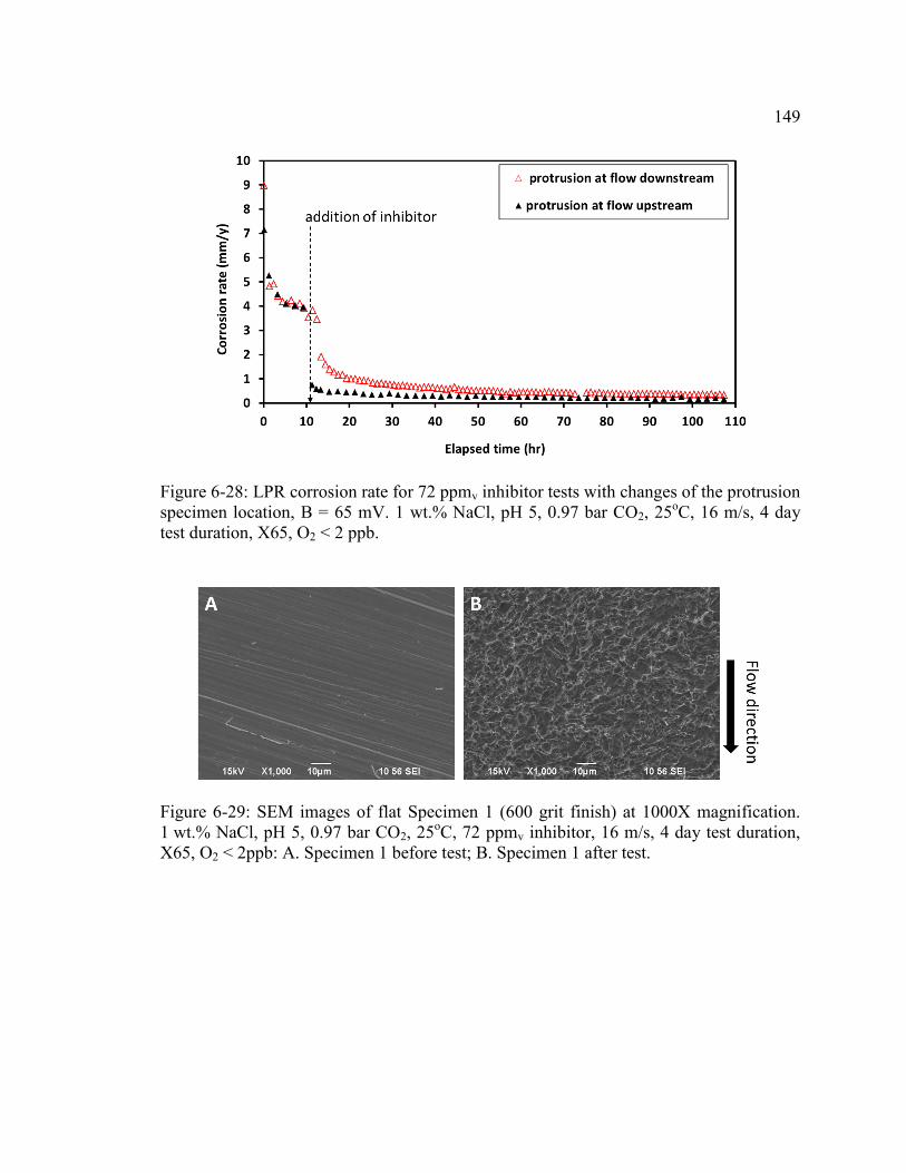
149
Figure 6-28: LPR corrosion rate for 72 ppmv inhibitor tests with changes of the protrusion specimen location, B = 65 mV. 1 wt.% NaCl, pH 5, 0.97 bar CO2, 25oC, 16 m/s, 4 day test duration, X65, O2 < 2 ppb.
Figure 6-29: SEM images of flat Specimen 1 (600 grit finish) at 1000X magnification. 1 wt.% NaCl, pH 5, 0.97 bar CO2, 25oC, 72 ppmv inhibitor, 16 m/s, 4 day test duration, X65, O2 < 2ppb: A. Specimen 1 before test; B. Specimen 1 after test.
150
Figure 6-30: SEM images of protrusion Specimen 3 on the most upstream port in the TCFC (port 1). Before test: 1st row at 50X magnification. After test: 2nd row at 50X magnification; 3rd row at 1000X magnification. Physical locations are defined by using 5 numbered individual regions in Figure 6-2. 1 wt.% NaCl, pH 5, 0.97 bar CO2, 25oC, 72 ppmv inhibitor, 16 m/s, 4 day test duration, X65, O2 < 2 ppb.
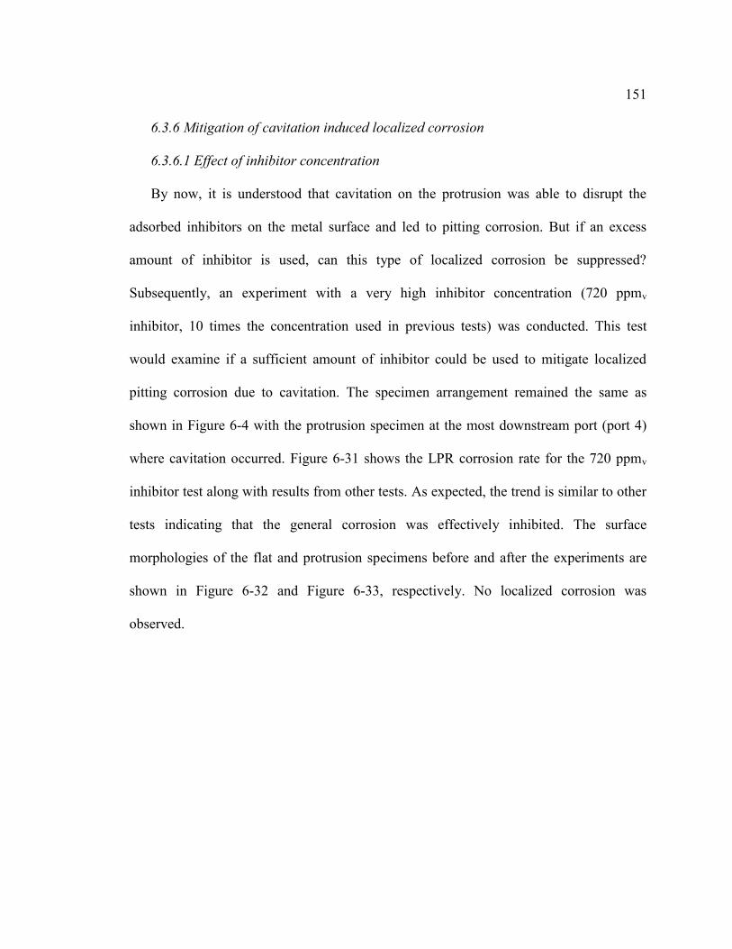
151
6.3.6 Mitigation of cavitation induced localized corrosion
6.3.6.1 Effect of inhibitor concentration
By now, it is understood that cavitation on the protrusion was able to disrupt the
adsorbed inhibitors on the metal surface and led to pitting corrosion. But if an excess
amount of inhibitor is used, can this type of localized corrosion be suppressed?
Subsequently, an experiment with a very high inhibitor concentration (720 ppmv
inhibitor, 10 times the concentration used in previous tests) was conducted. This test
would examine if a sufficient amount of inhibitor could be used to mitigate localized
pitting corrosion due to cavitation. The specimen arrangement remained the same as
shown in Figure 6-4 with the protrusion specimen at the most downstream port (port 4)
where cavitation occurred. Figure 6-31 shows the LPR corrosion rate for the 720 ppmv
inhibitor test along with results from other tests. As expected, the trend is similar to other
tests indicating that the general corrosion was effectively inhibited. The surface
morphologies of the flat and protrusion specimens before and after the experiments are
shown in Figure 6-32 and Figure 6-33, respectively. No localized corrosion was
observed.
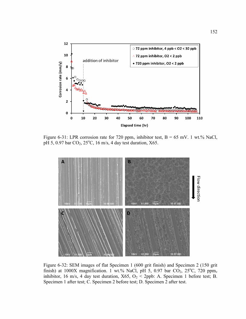
152
Figure 6-31: LPR corrosion rate for 720 ppmv inhibitor test, B = 65 mV. 1 wt.% NaCl, pH 5, 0.97 bar CO2, 25oC, 16 m/s, 4 day test duration, X65.
Figure 6-32: SEM images of flat Specimen 1 (600 grit finish) and Specimen 2 (150 grit finish) at 1000X magnification. 1 wt.% NaCl, pH 5, 0.97 bar CO2, 25oC, 720 ppmv inhibitor, 16 m/s, 4 day test duration, X65, O2 < 2ppb: A. Specimen 1 before test; B. Specimen 1 after test; C. Specimen 2 before test; D. Specimen 2 after test.
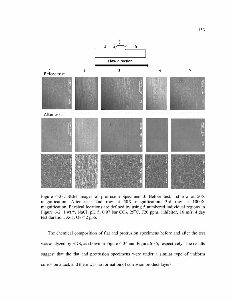
153
Figure 6-33: SEM images of protrusion Specimen 3. Before test: 1st row at 50X magnification. After test: 2nd row at 50X magnification; 3rd row at 1000X magnification. Physical locations are defined by using 5 numbered individual regions in Figure 6-2. 1 wt.% NaCl, pH 5, 0.97 bar CO2, 25oC, 720 ppmv inhibitor, 16 m/s, 4 day test duration, X65, O2 < 2 ppb.
The chemical composition of flat and protrusion specimens before and after the test
was analyzed by EDS, as shown in Figure 6-34 and Figure 6-35, respectively. The results
suggest that the flat and protrusion specimens were under a similar type of uniform
corrosion attack and there was no formation of corrosion product layers.
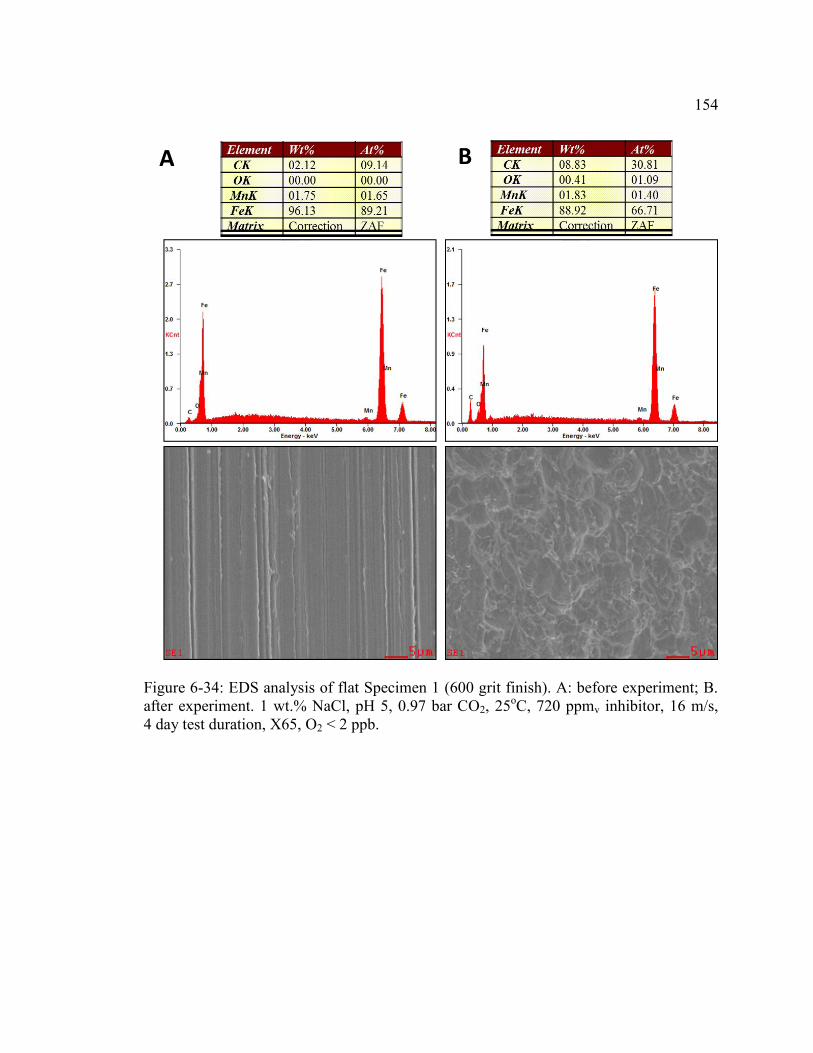
154
Figure 6-34: EDS analysis of flat Specimen 1 (600 grit finish). A: before experiment; B. after experiment. 1 wt.% NaCl, pH 5, 0.97 bar CO2, 25oC, 720 ppmv inhibitor, 16 m/s, 4 day test duration, X65, O2 < 2 ppb.
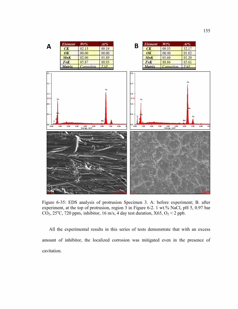
155
Figure 6-35: EDS analysis of protrusion Specimen 3. A: before experiment; B. after experiment, at the top of protrusion, region 3 in Figure 6-2. 1 wt.% NaCl, pH 5, 0.97 bar CO2, 25oC, 720 ppmv inhibitor, 16 m/s, 4 day test duration, X65, O2 < 2 ppb.
All the experimental results in this series of tests demonstrate that with an excess
amount of inhibitor, the localized corrosion was mitigated even in the presence of
cavitation.
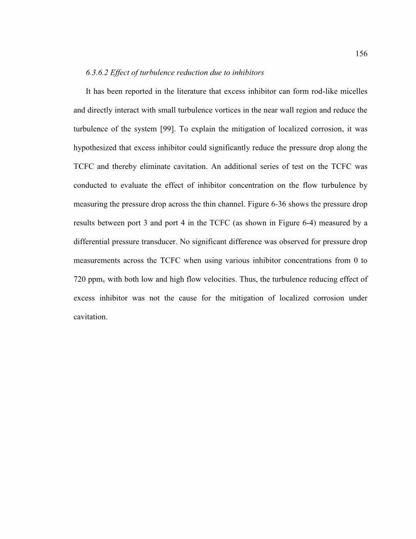
156
6.3.6.2 Effect of turbulence reduction due to inhibitors
It has been reported in the literature that excess inhibitor can form rod-like micelles
and directly interact with small turbulence vortices in the near wall region and reduce the
turbulence of the system [99]. To explain the mitigation of localized corrosion, it was
hypothesized that excess inhibitor could significantly reduce the pressure drop along the
TCFC and thereby eliminate cavitation. An additional series of test on the TCFC was
conducted to evaluate the effect of inhibitor concentration on the flow turbulence by
measuring the pressure drop across the thin channel. Figure 6-36 shows the pressure drop
results between port 3 and port 4 in the TCFC (as shown in Figure 6-4) measured by a
differential pressure transducer. No significant difference was observed for pressure drop
measurements across the TCFC when using various inhibitor concentrations from 0 to
720 ppmv with both low and high flow velocities. Thus, the turbulence reducing effect of
excess inhibitor was not the cause for the mitigation of localized corrosion under
cavitation.
157
Figure 6-36: Pressure drop measurements between port 3 and port 4 in the TCFC with various inhibitor concentrations. 1 wt.% NaCl, pH 5, 0.97 bar CO2, 25oC.
So far, without a doubt, it was found that cavitation led to inhibitor failure at 72 ppmv
and caused pitting corrosion, while this did not happen by using 720 ppmv of the same
inhibitor under the same experimental conditions. The mechanism related to this
phenomenon is discussed in the next section.
6.4 Discussion
In this work, it was found that the WSS of the order of 103 Pa introduced by the
highly turbulent single phase flow with a locally disturbed flow by a surface protrusion
was unable to affect the corrosion inhibitor adsorption/desorption process on a steel
surface. This is in line with other authors’ experimental observations [17] and
calculations that a much higher stress or energy would be needed to disrupt the inhibitor
films adsorbed on a steel surface [22].
158
6.4.1 Effect of pre-corrosion on corrosion inhibition at high flow velocity
Different surface polishing treatments on the steel surface did not influence the
inhibitor performance as evidenced by similar corrosion behaviors of Specimen 1 (600
grit sand paper polished) and Specimen 2 (150 grit sand paper polished). This was due to
the pre-corrosion procedure during the experiments. In order to obtain a stable blank
corrosion rate before an addition of inhibitor, the pre-corrosion periods were generally 10
to 12 hours in these tests. It was possible that a uniformly corroded steel surface was
created in the presence of such a high flow velocity (high uniform corrosion rate)
regardless of the initial surface polish. It has been reported that pre-corrosion on a steel
surface generally impaired the inhibitor performance at relative low flow velocity (1 m/s)
due to the formation of a cementite layer on the steel surface [100]. However, in the
presented work, the detrimental effect of pre-corrosion due to the formation of a
cementite layer was unlikely. This is because the formed cementite was probably
mechanically removed by the high general WSS and local WSS fluctuations (order of
103 Pa).
6.4.2 B value at high flow velocity
In this study, weight loss and LPR measurements were used to determine the
corrosion rates. The weight loss results gave an accurate time-averaged corrosion rate but
with no indication of momentary corrosion rate changes when the inhibitor was added.
LPR is a suitable technique for online corrosion rate monitoring and is capable of
capturing the transients with the addition of an inhibitor. However, a suitable B value

159
needs to be determined in order to obtain correct instantaneous corrosion rates. A B value
of 65 mV was used throughout the present tests for LPR corrosion rate calculation. The B
value was calibrated through the blank test and was assumed unchanged after the addition
of inhibitor. It is noted that this B value is much larger than the typical value in a CO2
corrosion system (e.g., B= 26 mV). This is because the limiting current for H+ reduction
in the present study was drastically enhanced by the high flow velocity, which increased
the cathodic reaction rate. It is found in the literature that the CO2 corrosion rate at pH 5
is flow dependent due to the increase of mass transfer controlled H+ reduction reaction
[64]. The calculated large B value indicates that the cathodic reaction is to some extent
controlled by the mass transfer process. The time-averaged corrosion rate that is
calculated from the LPR technique by integrating the area underneath the corrosion rate –
time curve are compared with the averaged corrosion rates calculated from weight losses
of specimens, as shown in Figure 6-37. The corrosion rates are generally coherent except
for the 720 ppmv test, where the corrosion rate from LPR is much larger than the weight
loss corrosion rate. This discrepancy may be due to the measurement error from that
individual test.

160
Figure 6-37: Corrosion rates calculated from averaged weight losses of specimens and from LPR corrosion rate curves with B = 65 mV. 1 wt.% NaCl, pH 5, 0.97 bar CO2, 25oC, 16 m/s, 4 day test duration, X65.
6.4.3 Mechanisms of flow cavitation induced pitting corrosion and its mitigation
6.4.3.1 Effects of flow on inhibitor adsorption / desorption equilibrium
In this research, it was found that pitting corrosion occurred at the leading edge and at
the top of the protrusion in the presence of 72 ppmv inhibitor with local flow velocities up
to 28 m/s. With an excess amount of inhibitor (720 ppmv), this pitting corrosion was
mitigated under the same environmental and flow conditions. The pitting corrosion was
determined to be caused by local flow cavitation using experimental and computational
evidence. However, the effect of inhibitor concentration on the mitigation of this
cavitation induced pitting corrosion is not yet clear. Unlike the mechanical removal of a
solid corrosion product layer by high hydrodynamic stresses produced by flow, the
interactions between flow stresses and inhibitor films are less straightforward. As
discussed, the collapsed cavitation bubbles may generate significantly high stresses that
161
locally remove inhibitor molecules from the steel surface. The mechanical impacts of
collapsing bubbles onto a surface can reach MPa, even GPa magnitude [101,102].
Undoubtedly, this stress exceeds the adhesion strength of the inhibitor films to the steel
surface and mechanical removal of inhibitor is expected. However, the inhibitor
adsorption / desorption process on a steel surface is not static, but is considered to be in a
dynamic equilibrium. The adsorption kinetics of inhibitors is usually fast, especially in
this highly turbulent flow where the mass transfer is significantly enhanced. It is not easy
to interpret why the inhibitors on the steel surface, which were mechanically removed by
flow, were not replenished by the remaining inhibitors readily available in the bulk
solution. Instead of a standpoint derived from flow hydrodynamics, it may be useful to
discuss the flow effects on corrosion inhibition in relation to adsorption / desorption
reaction equilibria.
Experimental results from various researchers suggest that the adsorption of
imidazoline-type inhibitors follows the Langmuir adsorption model [4,93,103,104]. Thus,
the adsorption and desorption rates of the inhibitor (𝑅𝑎𝑑𝑠 and 𝑅𝑑𝑒𝑠) are simply written as:
𝑅𝑎𝑑𝑠 = 𝑘𝑎𝑑𝑠(1 − 𝜃)𝑐𝑖𝑛ℎ𝑖𝑏𝑏 (6-4)
𝑅𝑑𝑒𝑠 = 𝑘𝑑𝑒𝑠𝜃 (6-5)
where 𝑘𝑎𝑑𝑠 and 𝑘𝑑𝑒𝑠 are the reaction rate constants for adsorption and desorption
processes, respectively; 𝑐𝑖𝑛ℎ𝑖𝑏𝑏 is the inhibitor concentrations in the bulk; θ is the surface
coverage of inhibitor (0 < θ < 1). At equilibrium, the adsorption and desorption rates
should be equal, which yields:
𝑘𝑎𝑑𝑠(1 − 𝜃)𝑐𝑖𝑛ℎ𝑖𝑏𝑏 = 𝑘𝑑𝑒𝑠𝜃 (6-6)
162
Rearrangement of Equation (6-6) for a single equilibrium constant results in:
(1
𝜃− 1) 𝑐𝑖𝑛ℎ𝑖𝑏
𝑏 =1
𝐾 (6-7)
where 𝐾 is the inhibitor adsorption equilibrium constant, defined as:
𝐾 =𝑘𝑎𝑑𝑠
𝑘𝑑𝑒𝑠 (6-8)
The explanation for a series of small pits found along the leading edge of the
protrusion specimen is straightforward. As discussed in previous sections, formation of
cavitation bubbles at this location created large areas of gas-liquid interface and
consumed a fraction of the inhibitors which are amphiphilic and tend to aggregate at any
available interface. This led to a local depletion of inhibitor and caused localized
corrosion due to the incomplete inhibitor coverage on the steel surface. Consideration
from the view of adsorption / desorption reaction equilibria draws the same conclusion.
From Equation (6-7), if the bulk concentration of inhibitor (𝑐𝑖𝑛ℎ𝑖𝑏𝑏 ) is reduced due to the
consumption by cavitation bubbles, and if the adsorption equilibrium constant ( 𝐾 )
remains unchanged, the only way to hold the balance in this equation is to have a
decreasing surface coverage of inhibitor (θ), which results in a local depletion of
inhibitor.
In the present research, the majority of pits were found at the top of the protrusion
region, where the cavitation bubble implosions presumably occurred. Bubble collapses at
the top of the protrusion are supported by fundamental calculations. The streamwise
length at the top of the protrusion region is approximately 4 mm. When assuming that the
bubbles obtain the streamwise core flow velocity of 25 m/s (Figure 6-24), the time for

163
bubbles to travel across the top of the protrusion region would be approximately 160 µs.
This is generally coherent with findings in the literature that the collapse time of
cavitation bubbles vary from 100 µs to a few ms [102,105,106]. Thus, bubble collapses
on top of the protrusion would occur, as also were corroborated by the present
experimental results.
The dynamics of cavitation bubbles near a solid wall have been extensively
researched [101,102,107–109]. During bubble collapses, the potential energy of vaporous
bubbles is converted into mechanical energy (including shock waves), heat, chemical
energy, sound and light emissions [101,110]. It is assumed that the energy releases in
various forms during bubble collapses negatively affect the inhibitor adsorption
equilibrium constant (𝐾) by enhancing the desorption reaction (increasing the 𝑘𝑑𝑒𝑠 ),
which results in a decreasing surface coverage of inhibitor according to Equation (6-7).
As discussed, the high mechanical stresses generated by collapsing bubbles can
directly remove the adsorbed inhibitors on the steel surface, which essentially facilitates
the desorption reaction. Because of that, the overall inhibitor adsorption equilibrium
would shift to the direction of desorption reaction, leading to the local depletion of
inhibitor and localized corrosion.
Besides the high magnitude of mechanical energy, collapsing cavitation bubbles can
also release an enormous amount of heat (thermal energy) and even emit light [111–113].
The temperature surrounding the collapsing cavitation bubbles can reach several
thousands of Kelvins (K) [110,114]. It is also possible that some of the released heat is
also transferred to the steel surface, resulting in local temperature increase. It is found in
164
the literature that the desorption reaction of imidazoline-type inhibitors is favorable when
the surface temperature increases [4,103,115]. From Equation (6-7), if the 𝐾 decreases
and the bulk concentration of inhibitor remains the same, the surface coverage has to
decrease to balance this equation.
6.4.3.2 Energy consideration in the thin channel flow cell system
As mentioned earlier, it is assumed that the flow can negatively affect the inhibitor
adsorption/desorption reaction equilibrium by enhancing the desorption reaction rate.
Several forms of energy are involved in this process and are discussed below.
The reaction equilibrium is controlled by the chemical thermodynamics. A vast
amount of research has been conducted focusing on the thermodynamic properties of
inhibitor adsorption reactions. For example, it has been generally accepted that the
standard free energy change due to surfactant inhibitor adsorption reaction (∆𝑟𝑥𝑛𝐺𝑜) is
approximately -40 kJ to -20 kJ per mole of adsorbed inhibitors [116,117], which suggests
that the adsorption reaction is thermodynamically favored at standard conditions.
The reaction rate of inhibitor adsorption is controlled by the chemical kinetics. The
kinetic activation energy of the inhibitor adsorption reaction (∆𝐺𝑎𝑑𝑠) is estimated to be
approximately 19 ± 2 kJ per mole of inhibitor [118,119]. The relationship between the
thermodynamic and kinetic energy changes due to the inhibitor adsorption/desorption
process can be illustrated by an energy diagram (as shown in Figure 6-38). From this
diagram, it can be seen that the desorption process has a much larger activation energy
(∆𝐺𝑑𝑒𝑠) than the adsorption reaction. Obviously, if the flow would affect the inhibitor
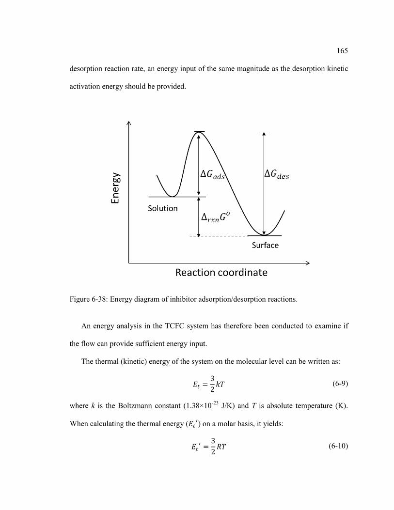
165
desorption reaction rate, an energy input of the same magnitude as the desorption kinetic
activation energy should be provided.
Figure 6-38: Energy diagram of inhibitor adsorption/desorption reactions.
An energy analysis in the TCFC system has therefore been conducted to examine if
the flow can provide sufficient energy input.
The thermal (kinetic) energy of the system on the molecular level can be written as:
𝐸𝑡 =3
2𝑘𝑇 (6-9)
where k is the Boltzmann constant (1.38×10⁻²³ J/K) and T is absolute temperature (K).
When calculating the thermal energy (𝐸𝑡′) on a molar basis, it yields:
𝐸𝑡′ =
3
2𝑅𝑇 (6-10)
166
where R is the gas constant (8.314 J/K∙mole).
Besides random motions of the molecules, there is also an ordered directional
movement of the liquid molecules in a flow system, referred to as the bulk flow velocity.
The additional kinetic energy (𝐸𝑘) due to the directional flow can be written as:
𝐸𝑘 =1
2𝑚𝑣2 (6-11)
where m is the molar mass of the liquid molecules (kg/mole); and 𝑣 is the flow
velocity (m/s).
The bulk temperature in the TCFC was 298 K, while the flow stream velocity on the
top of the protrusion was 25 m/s (Figure 6-24). According to Equation (6-10) and (6-11),
the thermal energy and flow kinetic energy are calculated to be 3.7 kJ and 5.6 J per mole
of water, respectively.
The Langmuir adsorption of inhibitor is essentially the displacement of adsorbed
water molecules at the steel surface, as given by [120]:
𝑖𝑛ℎ𝑖𝑏𝑖𝑡𝑜𝑟 (𝑠𝑜𝑙) + 𝐻2𝑂(𝑎𝑑𝑠) ⇌ 𝑖𝑛ℎ𝑖𝑏𝑖𝑡𝑜𝑟 (𝑎𝑑𝑠) + 𝐻2𝑂(𝑠𝑜𝑙) (6-12)
Because the stoichiometric coefficients for all substances in this reaction are equal,
the molar energies of inhibitor adsorption and water flow can be directly comparable. It
shows that the energy level of the bulk flow kinetic energy (only several J/mole) is
several orders of magnitude smaller than the adsorption/desorption activation energies
(several kJ/mole). It may be therefore concluded that the energy due to bulk flow in the
TCFC (e.g., wall shear stress) could not affect the inhibitor adsorption/desorption
process.
167
Although bulk flow seems unable to provide enough energy to affect inhibitor
adsorption/desorption processes, the collapses of cavitating bubbles in the TCFC may do
so. The total potential energy by a single spherical cavitation bubble is given by [102]:
𝐸𝑝 =4
3𝜋𝑟3(𝑃∞ − 𝑃𝑣) (6-13)
where 𝑃∞ is the ambient pressure at infinite distance; 𝑃𝑣 is the vapor pressure of the
liquid; 𝑟 is the bubble radius; and 𝐸𝑝 is the bubble potential energy. The potential energy
on a molar basis may be written as:
𝐸𝑝′ =𝑚
𝜌𝑣
(𝑃∞ − 𝑃𝑣) (6-14)
where m is the molar mass of the liquid (kg/mole); and 𝜌𝑣 is the vapor density of the
liquid (kg/m3). At 298 K, the vapor pressure and vapor density of water are 3200 Pa and
0.024 kg/m3 (ideal gas law), respectively. The ambient pressure at infinite distance in the
TCFC is 1×10⁵ Pa. Consequently, the bubble potential energy is calculated to be 72.6 kJ
per mole of water vapor, which is much larger than the energy levels of inhibitor
adsorption reactions.
The collapsing cavitation bubbles with their various forms of energy releases,
particularly the mechanical energy release, undoubtedly reach the magnitude of the
inhibitor desorption activation energy. It is therefore proposed that the desorption
activation energy is decreased as the surface energy level is increased due to the energy
input from collapsing cavitation bubbles (shown in Figure 6-39).
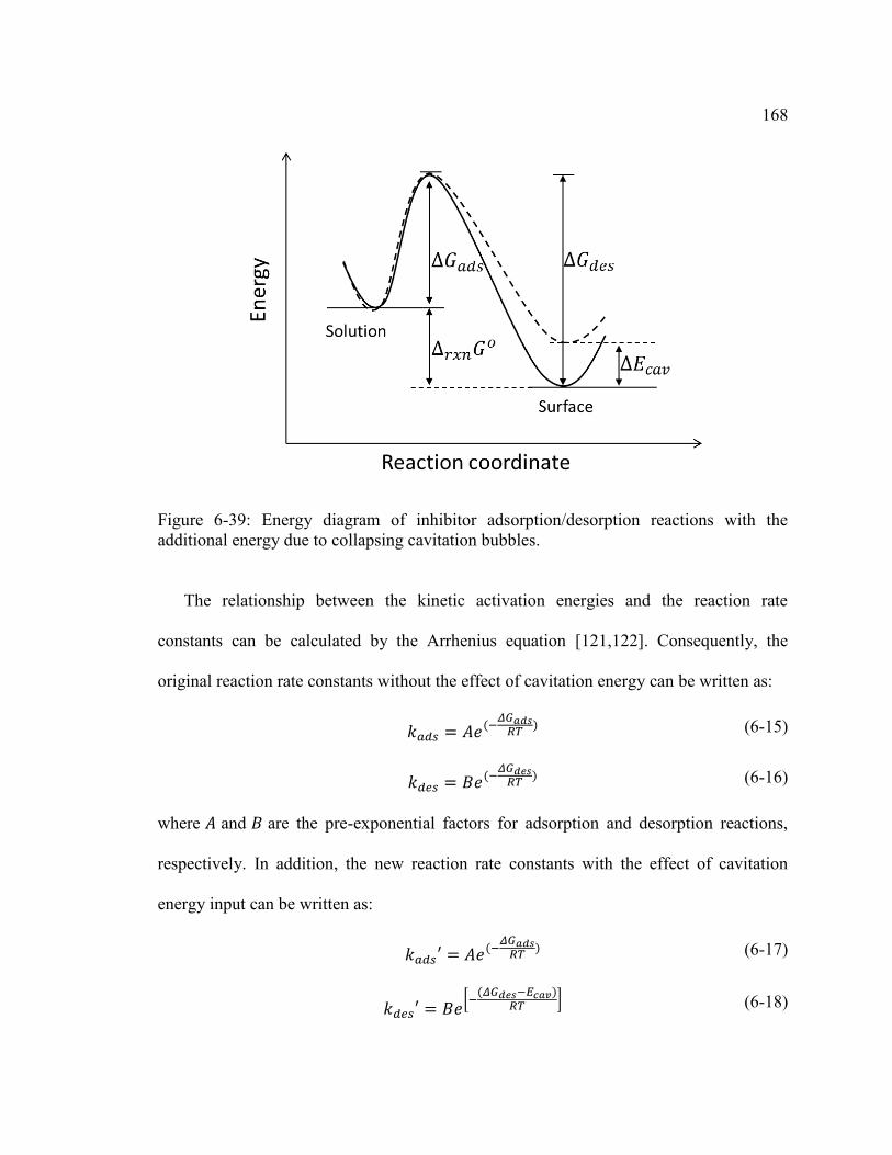
168
Figure 6-39: Energy diagram of inhibitor adsorption/desorption reactions with the additional energy due to collapsing cavitation bubbles.
The relationship between the kinetic activation energies and the reaction rate
constants can be calculated by the Arrhenius equation [121,122]. Consequently, the
original reaction rate constants without the effect of cavitation energy can be written as:
𝑘𝑎𝑑𝑠 = 𝐴𝑒(−𝛥𝐺𝑎𝑑𝑠
𝑅𝑇) (6-15)
𝑘𝑑𝑒𝑠 = 𝐵𝑒(−𝛥𝐺𝑑𝑒𝑠
𝑅𝑇) (6-16)
where 𝐴 and 𝐵 are the pre-exponential factors for adsorption and desorption reactions,
respectively. In addition, the new reaction rate constants with the effect of cavitation
energy input can be written as:
𝑘𝑎𝑑𝑠′ = 𝐴𝑒(−𝛥𝐺𝑎𝑑𝑠
𝑅𝑇) (6-17)
𝑘𝑑𝑒𝑠′ = 𝐵𝑒[−
(𝛥𝐺𝑑𝑒𝑠−𝐸𝑐𝑎𝑣)𝑅𝑇
] (6-18)

169
where 𝐸𝑐𝑎𝑣 is the energy input due to collapsing cavitation bubbles. When substituting
these reaction rate constants into Equation (6-8), it reveals that the adsorption/desorption
reaction equilibrium shifts to the direction of desorption reaction (𝐾′ < 𝐾). According to
Equation (6-7), when the equilibrium constant decreases and the bulk inhibitor
concentration is unchanged, the surface coverage of inhibitor has to decrease, which
explains the inhibitor failure at 72 ppmv.
From the energy analysis, a same postulate can be made that the bulk flow seen in
typical systems is very unlikely to affect the inhibitor adsorption/desorption process.
However, the physical effects of collapses of cavitation bubbles, e.g., releases of high
magnitude mechanical energy and thermal energy, may influence the inhibitor
adsorption/desorption equilibrium.
6.4.3.3 Mitigation of cavitation induced localized corrosion
It has been shown above that collapsing cavitation bubbles affect the inhibitor
adsorption/desorption equilibrium by facilitating the desorption process, which leads to a
decreasing coverage of inhibitor on the steel surface and induces localized corrosion.
From Equation (6-7), a higher bulk concentration of inhibitor (𝑐𝑖𝑛ℎ𝑖𝑏𝑏 ) would be required
in order to maintain a sufficient surface coverage of inhibitor and mitigate the localized
corrosion. This was corroborated by the experimental results that an excess amount of
inhibitor (720 ppmv) mitigated the cavitation induced localized corrosion at the
protrusion.

170
In a nutshell, collapsing cavitation bubbles disrupt the original inhibitor
adsorption/desorption equilibrium by enhancing the desorption process, which results in a
decreasing surface coverage of inhibitor. Excess inhibitor reverses this situation by
enhancing the inhibitor adsorption process and thereby mitigates cavitation induced
localized corrosion.
6.4.4 Microscopic expressions for continuum hydrodynamics
The present study shows that some flow conditions can mechanically affect the
inhibitor adsorption/desorption equilibrium by hydrodynamic stresses, e.g., impacts of
shock waves due to cavitation bubble implosions. However, the link between bulk flow
hydrodynamics and inhibitor behaviors on the surface is not yet established. The inhibitor
adsorption/desorption process occurs at molecular length scales (order of nm), which are
much smaller than the spatial resolution of continuum hydrodynamics. A means to
connect the macroscopic and molecular hydrodynamics is crucial in order to interpret the
interactions between bulk flow and inhibitor molecules. Fortunately, such a bridge has
already been built, for example, by molecular dynamics simulation (MD) [123,124].
In molecular dynamics simulation, the movements of individual molecules in the
simulated system are governed by prescribed intermolecular potentials. The time
evolution of the system is obtained by solving Newton’s equations of motion for all the
molecules [123]. By averaging the quantities of molecules, such as their trajectories and
intermolecular potentials, the continuum hydrodynamic properties may be obtained
171
[124]. For example, the microscopic expression of the shear stress tensor may be given
by [123]:
𝜏𝑥𝑦 =1
𝑉[∑ 𝑚(𝑣𝑥𝑖 − �̅�𝑥)(𝑣𝑦𝑖 − �̅�𝑦) +
𝑖
1
2∑ ∑ 𝑥𝑖𝑗
𝜕𝑢(𝒓𝑖𝑗)
𝜕𝑦𝑖𝑗
𝑁
𝑗≠𝑖=1
𝑁
𝑖=1
] (6-19)
where 𝒓𝑖𝑗 is the trajectory between molecule 𝑖 and 𝑗; 𝑢 is the intermolecular potential; 𝑥𝑖𝑗
and 𝑦𝑖𝑗are projections of 𝒓𝑖𝑗 in x and y directions; 𝑣𝑥𝑖 and 𝑣𝑦𝑖 are velocities of molecule 𝑖
in x and y directions; �̅�𝑥 and �̅�𝑦 are the averaged velocities of all molecules in x and y
directions; 𝑚 is the mass of molecule; and 𝑉 is the volume of the simulated system.
Molecular dynamics simulation bridges the gap between measured macroscopic
hydrodynamic quantities and the motions of individual molecules beneath the length and
time scales of continuum fluid mechanics. Therefore, molecular dynamics simulation can
be used for future research as a diagnostic tool to investigate the effects of bulk flow on
inhibitor adsorption/desorption processes.
6.5 Summary
Mechanical removal of inhibitor by flow cavitation was confirmed. Based on the
presented results and discussion, the findings can be summarized as:
Specimens protruded into the flow stream drastically changed the local
hydrodynamic conditions and caused cavitation in a highly turbulent flow system.
The protrusion led to a local wall shear stress up to 4.8 kPa in the studied flow
conditions. However, an effect of wall shear stress on the inhibitor
adsorption/desorption process was not observed. This is because the wall shear

172
stress, even in “extreme” flow conditions, is several orders of magnitude lower
than the adhesion strength of inhibitor films to the steel surface.
The inhibitor adsorption/desorption equilibrium was significantly influenced by
the collapsing cavitation bubbles, which enhanced the inhibitor desorption
process, reduced the surface coverage of inhibitor, and caused localized corrosion
due to local inhibitor depletion.
An excess amount of inhibitor eliminated the cavitation induced localized
corrosion by establishing a new adsorption/desorption equilibrium and
maintaining a sufficient surface coverage of inhibitor.
173
Chapter 7: Conclusions and Recommendations
7.1 Conclusions
In the research reported in this dissertation, the mechanical effects of flow on CO2
corrosion inhibition of carbon steel pipelines have been investigated. The experimental
studies mainly focused on two main topics: hydrodynamics relating to wall shear stress
measurement in flow pipelines encountered CO2 corrosion problems and failure of
corrosion inhibition due to mechanical effects of extremely turbulent flow. Several
conclusions based on the present research can be drawn:
The floating element method was successful in directly measuring wall shear
stress in the studied flow, which provides a new means for building better
understanding of complex multiphase flow.
In the studied multiphase flow patterns at ambient conditions, the highest wall
shear stress occurred in the slug flow pattern on the top of the pipe when the slug
front passed with the maximum in situ flow velocity.
The maximum wall shear stress in slug flow can be evaluated by current flow
modeling when a proper resolution of the local flow velocity profile is achieved.
The maximum shear stress value was about 2 to 4 times higher than the calculated
mean shear stress of the slug body using mixture velocity. This can serve as a
guideline for improving slug flow modeling with applications to other areas, such
as removal of corrosion inhibitor films and corrosion product layers.
In the studied flow at ambient conditions, the maximum wall shear stress value
for any horizontal two-phase flow pattern was of an order of 100 Pa, the value for
174
single-phase liquid flow did not exceed 1000 Pa. These stress values are several
orders of magnitude lower than the reported adhesion strength of inhibitor films
or FeCO3 layers. This suggests that mechanical removal of these films or layers
solely by wall shear stress typically seen in flow lines is very unlikely.
Results from corrosion inhibitor experiments and flow simulations at high flow
velocity conditions confirmed that a local wall shear stress up to 4.8 kPa could not
affect the protectiveness of corrosion inhibitor films on the steel surface.
A flow disturbance caused by surface protrusion significantly changed the local
hydrodynamics and caused flow cavitation at a high flow velocity.
In laboratory experiments, flow cavitation was identified as being able to
mechanically affect corrosion inhibitor films and cause localized corrosion.
The inhibitor adsorption/desorption equilibrium was significantly influenced by
the collapsing cavitation bubbles, which generated a mechanical stress that
exceeds the magnitude of the adhesion strength of inhibitor, enhanced the
inhibitor desorption process, and caused localized corrosion due to local inhibitor
depletion.
An excess amount of inhibitor eliminated the cavitation induced localized
corrosion by establishing a new adsorption/desorption equilibrium and
maintaining a high surface coverage of inhibitor.

175
7.2 Recommendations
This dissertation focuses on the hydrodynamics of extremely turbulent flow and the
mechanical interactions between flow and CO2 corrosion inhibition, both of which are
complex. Although most of the initial research questions have been answered, some other
aspects related to these topics have been identified in the present research, and should be
taken into account for further investigation. Some recommendations are given below:
The floating element probe provides direct and accurate measurements of wall
shear stress fluctuations of relatively large time scale transients in single-phase
and multiphase flow, e.g, the passage of slugs. However, a floating element probe
with both high temporal and spatial resolutions may be necessary in order to
investigate the local wall shear stress fluctuations due to the smallest turbulent
eddies.
The present research shows that a proper resolution of the flow field is essential
for building understanding of multiphase flow, including evaluation of wall shear
stress. Future research may focus on obtaining the complete flow velocity profile
in multiphase flow patterns through experiments and/or computational
simulations.
Although a number of different multiphase flow patterns have been studied in the
present research, some specific flow conditions found in the field, involving a
discrete phase, were not covered. For example, entrained liquid droplets in
annular-mist flow, that travel at high gas velocities, can lead to high energy wall
impacts (high local mechanical stresses), particularly at locations of disturbed
176
flow, such as bends, valves, tees, weld beads, etc. A proper evaluation of the
mechanical stresses during the impacts through experimental research or
numerical simulation would be needed to assess the mechanical effect of discrete
phases on corrosion inhibition.
The present experimental research undoubtedly demonstrates that some flow
conditions can mechanically affect inhibitor adsorption/desorption equilibria.
However, the link between the macroscopic flow behavior and the microscopic
inhibitor adsorption/desorption process is not fully understood. Future
investigation may use computer simulation approaches, for example, such as
molecular dynamics simulation, in order to connect the macroscopic laboratory
experiments to the microscopic behaviors of inhibitor molecules.
177
References
[1] U.S. Liquids Pipeline Usage & Mileage Report, Association of Oil Pipe Lines
(AOPL) and American Petroleum Institute (API), November 2015.
[2] S. Nesic, W. Sun, Corrosion in acid gas Solutions, in: J.A. Richardson, et al.
(Eds.), Shreir’s Corrosion, Elsevier, Amsterdam, The Netherlands, 2010, pp.
1270–1298.
[3] S. Nesic, Carbon dioxide corrosion of mild steel, in: R. Winston Revie (Ed.),
Uhlig’s Corrosion Handbook, third ed., John Wiley & Sons, Inc., Hoboken, New
Jersey, 2011, pp. 229–245.
[4] S. Ramachandran, B.-L. Tsai, M. Blanco, H. Chen, Y. Tang, W.A. Goddard III,
Self-assembled monolayer mechanism for corrosion inhibition of iron by
imidazolines, Langmuir 12 (1996) 6419–6428.
[5] T. Li, Y. Yang, K. Gao, M. Lu, Mechanism of protective film formation during
CO2 corrosion of X65 pipeline steel, J. Univ. Sci. Technol. Beijing 15 (2008) 702–
706.
[6] W. Li, B. Brown, D. Young, S. Nesic, Investigation of pseudo-passivation of mild
steel in CO2 corrosion, Corrosion 70 (2014) 294–302.
[7] J. Zhang, Z.L. Wang, Z.M. Wang, X. Han, Chemical analysis of the initial
corrosion layer on pipeline steels in simulated CO2-enhanced oil recovery brines,
Corros. Sci. 65 (2012) 397–404.
[8] J. Han, D. Young, H. Colijn, A. Tripathi, S. Nesic, Chemistry and structure of the
passive film on mild steel in CO2 corrosion environments, Ind. Eng. Chem. Res. 48
(2009) 6296–6302.

178
[9] R.H. Hausler, G. Schmitt, Hydrodynamic and flow effects on corrosion inhibition,
in: NACE International CORROSION 2004 conference, 2004, paper no. 04402.
[10] S. Nesic, Effects of multiphase flow on internal CO2 corrosion of mild steel
pipelines, Energy Fuels 26 (2012) 4098–4111.
[11] K. Gao, F. Yu, X. Pang, G. Zhang, L. Qiao, W. Chu, M. Lu, Mechanical properties
of CO2 corrosion product scales and their relationship to corrosion rates, Corros.
Sci. 50 (2008) 2796–2803.
[12] V. Ruzic, M. Veidt, S. Nesic, Protective iron carbonate films – part 1: mechanical
removal in single-phase aqueous flow, Corrosion. 62 (2006) 419–432.
[13] G. Schmitt, M. Mueller, Critical wall shear stresses in CO2 corrosion of carbon
steel, in: NACE International CORROSION 99 conference, 1999, paper no. 44.
[14] B.F.M. Pots, E.L.J.A. Hendriksen, H.A.M. de Reus, H.B. Pit, S.J. Paterson, Field
study of corrosion inhibition at very high flow velocity, in: NACE International
CORROSION 2003 conference, 2003, paper no. 03321.
[15] B. Poulson, Advances in understanding hydrodynamic effects on corrosion,
Corros. Sci. 35 (1993) 655–665.
[16] S. Seal, K. Sapre, A. Kale, V. Desai, M. Gopal, P. Jepson, Effect of multiphase
flow on corrosion of C-steel in presence of inhibitor: a surface morphological and
chemical study, Corros. Sci. 42 (2000) 1623–1634.
[17] E. Gulbrandsen, A. Grana, Testing of carbon dioxide corrosion inhibitor
performance at high flow velocities in jet impingement geometry. Effects of mass
transfer and flow forces, Corrosion 63 (2007) 1009–1020.
[18] F. Farelas, Thin channel flow cell study: mechanical and chemical removal of
FeCO3 scales in carbon steel, CCJIP Advisory Board Meeting, Institute for
Corrosion and Multiphase Technology, Ohio Univ., Athens, OH, November 2008.

179
[19] Y. Yang, B. Brown, S. Nesic, M. Elena Gennaro, B. Molinas, Mechanical strength
and removal of a protective iron carbonate layer formed on mild steel in CO2
corrosion, in: NACE International CORROSION 2010 conference, 2010, paper no.
10383.
[20] J. Huang, B. Brown, S. Nesic, Localized corrosion of mild steel under silica
deposits in inhibited aqueous CO2 solutions, in: NACE International
CORROSION 2013 conference, 2013, paper no. 2144.
[21] J.R. Shadley, S.A. Shirazi, E. Dayalan, E.F. Rybicki, Prediction of erosion-
corrosion penetration rate in a carbon dioxide environment with sand, Corrosion
54 (1998) 972–978.
[22] Y. Xiong, B. Brown, B. Kinsella, S. Nesic, A. Pailleret, Atomic force microscopy
study of the adsorption of surfactant corrosion inhibitor films, Corrosion 70 (2014)
247–260.
[23] G. Schmitt, C. Bosch, P. Plagemann, K. Moeller, Local wall shear stress gradients
in the slug flow regime – Effects of hydrocarbon and corrosion inhibitor, in:
NACE International CORROSION 2002 conference, 2002, paper no. 02244.
[24] V.E. Nakoryakov, O.N. Kashinsky, A.P. Burdukov, V.P. Odnoral, Local
characteristics of upward gas-liquid flows, Int. J. Multiphase Flow 7 (1981) 63–81.
[25] H. Wang, T. Hong, J.Y. Cai, W.P. Jepson, C. Bosch, Enhanced mass transfer and
wall shear stress in multiphase slug flow, in: NACE International CORROSION
2002 conference, 2002, paper no. 02501.
[26] T.K. Villiger, M. Morbidelli, M. Soos, Experimental determination of maximum
effective hydrodynamic stress in multiphase flow using shear sensitive aggregates,
AIChE J. 61 (2015) 1735–1744.
180
[27] D. Zheng, D. Che, Y. Liu, Experimental investigation on gas-liquid two-phase slug
flow enhanced carbon dioxide corrosion in vertical upward pipeline, Corros. Sci.
50 (2008) 3005–3020.
[28] J.W. Naughton, M. Sheplak, Modern developments in shear-stress measurement,
Prog. Aerospace Sci. 38 (2002) 515–570.
[29] T.J. Hanratty, J.A. Campbell, Measurement of wall shear stress, in: R.J. Goldstein
(Ed.), Fluid Mechanics Measurements, second ed., Taylor & Francis, Washington,
DC, 1996: pp. 575–649.
[30] J.F. Kiefner, C.J. Trench, Oil Pipeline Characteristics and Risk Factors:
Illustrations from the Decade of Construction, American Petroleum Institute (API),
December 2001.
[31] A. Danesh, PVT and Phase Behaviour of Petroleum Reservoir Fluids, Elsevier,
Amsterdam, The Netherlands, 1998.
[32] H.J. Herzog, What future for carbon capture and sequestration?, Environ. Sci.
Technol. 35 (2001) 148A–153A.
[33] J.C.M. Pires, F.G. Martins, M.C.M. Alvim-Ferraz, M. Simoes, Recent
developments on carbon capture and storage: An overview, Chem. Eng. Res. Des.
89 (2011) 1446–1460.
[34] S. Chu, Carbon capture and sequestration, Science 325 (2009) 1599.
[35] H.J. Herzog, E.M. Drake, Carbon dioxide recovery and disposal from large energy
systems, Annu. Rev. Energy Environ. 21 (1996) 145–166.
[36] Carbon Dioxide Enhanced Oil Recovery. Untapped Domestic Energy Supply and
Long Term Carbon Storage Solution, National Energy Technology Laboratory
(NETL), U.S. Department of Energy, March 2010.

181
[37] M.K. Verma, Fundamentals of Carbon Dioxide-Enhanced Oil Recovery (CO2-
EOR) – A Supporting Document of the Assessment Methodology for Hydrocarbon
Recovery Using CO2-EOR Associated with Carbon Sequestration, U.S. Geological
Survey, Open-File Report 2015-1071, 2015.
[38] J.P. Meyer, Summary of Carbon Dioxide Enhanced Oil Recovery (CO2EOR)
Injection Well Technology, American Petroleum Institute (API), 2005.
[39] M.B. Kermani, A. Morshed, Carbon dioxide corrosion in oil and gas production –
A compendium, Corrosion 59 (2003) 659–683.
[40] C. de Waard, D.E. Milliams, Carbonic acid corrosion of steel, Corrosion 31 (1975)
177–181.
[41] L.G.S. Gray, B.G. Anderson, M.J. Danysh, P.R. Tremaine, Mechanisms of carbon
steel corrosion in brines containing dissovled carbon dioxide at pH 4, in: NACE
International CORROSION 89 conference, 1989, paper no. 464.
[42] L.G.S. Gray, B.G. Anderson, M.J. Danysh, P.R. Tremaine, Effect of pH and
temperature on the mechanism of carbon steel corrosion by aqueous carbon
dioxide, in: NACE International CORROSION 90 conference, 1990, paper no. 40.
[43] S. Nesic, J. Postlethwaite, S. Olsen, An electrochemical model for prediction of
corrosion of mild steel in aqueous carbon dioxide solutions, Corrosion 52 (1996)
280–294.
[44] W. Sun, S. Nesic, R.C. Woollam, The effect of temperature and ionic strength on
iron carbonate (FeCO3) solubility limit, Corros. Sci. 51 (2009) 1273–1276.
[45] E. Gulbrandsen, J.-H. Morard, J.-L. Crolet, Study of the possible mechanisms of
steel passivation in CO2 corrosion, in: NACE International CORROSION 99
conference, 1999, paper no. 624.
182
[46] F.D. de Moraes, J.R. Shadley, J. Chen, E.F. Rybicki, Characterization of CO2
corrosion product scales related to environmental conditions, in: NACE
International CORROSION 2000 conference, 2000, paper no. 00030.
[47] V.S. Sastri, Corrosion Inhibitors: Principles and Applications., John Wiley & Sons,
Ltd, Chichester, England, 1998.
[48] B. Sanyal, Organic compounds as corrosion inhibitors in different environments –
A review, Prog. Org. Coatings 9 (1981) 165–236.
[49] M.W. Ranney, Corrosion Inhibitor. Manufacture and Technology, Noyes Data
Corporation, Park Ridge, New Jersey, 1976.
[50] M.A. Migahed, A.M. Al-Sabagh, Beneficial role of surfactants as corrosion
inhibitors in petroleum industry : a review article, Chem. Eng. Comm. 196 (2009)
1054–1075.
[51] M.J. Rosen, Surfactants and Interfacial Phennomena, third ed., John Wiley &
Sons, Inc., Hoboken, New Jersey, 2004.
[52] R. Fuchs-Godec, Effects of surfactants and their mixtures on inhibition of the
corrosion process of ferritic stainless steel, Electrochim. Acta 54 (2009) 2171–
2179.
[53] R. Zhang, P. Somasundaran, Advances in adsorption of surfactants and their
mixtures at solid/solution interfaces, Adv. Colloid Interface Sci. 123-126 (2006)
213–229.
[54] R. Atkin, Mechanism of cationic surfactant adsorption at the solid–aqueous
interface, Adv. Colloid Interface Sci. 103 (2003) 219–304.
[55] L.K. Koopal, E.M. Lee, M.R. Bohmer, Adsorption of cationic and anionic
surfactants on charged metal oxide surfaces, J. Colloid Interface Sci. 170 (1995)
85–97.

183
[56] P. Muller, Glossary of terms used in physical organic chemistry (IUPAC
Recommendations 1994), Pure Appl. Chem. 66 (1994) 1077–1184.
[57] D.A. Jones, Principles and Prevention of Corrosion, second ed., Prentice Hall,
Upper Saddle River, NJ, 1996.
[58] A. Edwards, C. Osborne, S. Webster, D. Klenerman, M. Joseph, P. Ostovar, M.
Doyle, Mechanistic studies of the corrosion inhibitor oleic imidazoline, Corros.
Sci. 36 (1994) 315–325.
[59] J.A. Martin, F.W. Valone, The existence of imidazoline corrosion inhibitors,
Corrosion 41 (1985) 281–287.
[60] N. Pebere, M. Duprat, F. Dabosi, A. Lattes, A. de Savignac, Corrosion inhibition
study of a carbon steel in acidic media containing hydrogen sulphide and organic
surfactants, J. Appl. Electrochem. 18 (1988) 225–231.
[61] A.J. McMahon, The mechanism of action of an oleic imidazoline based corrosion
inhibitor for oilfield use, Colloids Surf. 59 (1991) 187–205.
[62] O. Shoham, Mechanistic Modeling of Gas-Liquid Two-Phase Flow in Pipes,
Society of Petroleum Engineers, Richardson, Texas, 2006.
[63] S. Nesic, S. Wang, J. Cai, Y. Xiao, Integrated CO2 corrosion - multiphase flow
model, in: NACE International CORROSION 2004 conference, 2004, paper no.
04626.
[64] S. Nesic, G.T. Solvi, J. Enerhaug, Comparison of the rotating cylinder and pipe
flow tests for flow-sensitive carbon dioxide corrosion, Corrosion 51 (1995) 773–
787.
[65] L.P. Reiss, T.J. Hanratty, Measurement of instantaneous rates of mass transfer to a
small sink on a wall, AIChE J. 8 (1962) 245–247.

184
[66] G. Schmitt, C. Werner, M. Bakalli, Fluid mechanical interactions of turbulent
flowing liquids with the wall – revisited with a new electrochemical tool, in:
NACE International CORROSION 2005 conference, 2005, paper no. 05344.
[67] Z. Zhang, D. Hinkson, M. Singer, H. Wang, S. Nesic, A mechanistic model of top-
of-the-line corrosion, Corrosion 63 (2007) 1051–1062.
[68] K.G. Winter, An outline of the techniques available for the measurement of skin
friction in turbulent boundary layers, Prog. Aerospace Sci. 18 (1977) 1–57.
[69] L. Lofdahl, M. Gad-el-Hak, MEMS applications in turbulence and flow control,
Prog. Aerospace Sci. 35 (1999) 101–203.
[70] S. Tavoularis, Measurement in Fluid Mechanics, Cambridge University Press,
New York, NY, 2005.
[71] M.A. Schmidt, R.T. Howe, S.D. Senturia, J.H. Haritonidis, Design and calibration
of a microfabricated floating-element shear-stress Sensor, IEEE Trans. Electron.
Dev. 35 (1988) 750–757.
[72] A. Padmanabhan, H. Goldberg, K.D. Breuer, M.A. Schmidt, A wafer-bonded
floating-element shear stress microsensor with optical posititon sensing by
photodiodes, J. Microelectromech. Syst. 5 (1996) 307–315.
[73] J. Shajii, K.-Y. Ng, M.A. Schmidt, A microfabricated floating-element shear stress
sensor using wafer-bonding technology, J. Microelectromech. Syst. 1 (1992) 89–
94.
[74] V.A. Sheverev, V. Stepaniuk, Shear stress measurement apparatus, United States
patent no. US 8,276,463 B2, 2012.
[75] H. Ludwieg, W. Tillmann, Investigations of the Wall-Shearing Stress in Turbulent
Boundary Layers, National Advisory Committee for Aeronautics, Technical
Memorandum 1285, 1950.
185
[76] W. Li, Y. Xiong, B. Brown, K.E. Kee, S. Nesic, Measurement of wall shear stress
in multiphase flow and its effect on proctetive FeCO3 corrosion product layer
removal, in: NACE International CORROSION 2015 conference, 2015, paper no.
5922.
[77] W. Li, B.F.M. Pots, B. Brown, K.E. Kee, S. Nesic, A direct measurement of wall
shear stress in multiphase flow − Is it an important parameter in CO2 corrosion of
carbon steel pipelines?, Corros. Sci. http://dx.doi.org/10.1016/j.corsci.2016.04.008
[78] V.C. Patel, M.R. Head, Some observations on skin friction and velocity profiles in
fully developed pipe and channel flows, J. Fluid Mech. 38 (1969) 181–201.
[79] B.E. Launder, D.B. Spalding, The numerical computation of turbulent flows,
Comput. Methods Appl. Mech. Eng. 3 (1974) 269–289.
[80] G.A. Gregory, M.K. Nicholson, K. Aziz, Correlation of the liquid volume fraction
in the slug for horizontal gas-liquid slug flow, Int. J. Multiphase Flow. 4 (1978)
33–39.
[81] J.L. Rodgers, W.A. Nicewander, Thirteen ways to look at the correlation
coefficient, Am. Stat. 42 (1988) 59–66.
[82] N.I. Heywood, J.F. Richardson, Slug flow of air-water mixtures in a horizontal
pipe: determination of liquid holdup by γ-ray absorption, Chem. Eng. Sci. 34
(1979) 17–30.
[83] B.D. Woods, Z. Fan, T.J. Hanratty, Frequency and development of slugs in a
horizontal pipe at large liquid flows, Int. J. Multiphase Flow. 32 (2006) 902–925.
[84] G.A. Gregory, D.S. Scott, Correlation of liquid slug velocity and frequency in
horizontal cocurrent gas-liquid slug flow, AIChE J. 15 (1969) 933–935.
[85] G.J. Zabaras, Prediction of slug frequency for gas/liquid flows, SPE J. 5 (2000)
252–258.
186
[86] Y. Taitel, A.E. Dukler, A model for slug frequency during gas-liquid flow in
horizontal and near horizontal pipes, Int. J. Multiphase Flow. 3 (1977) 585–596.
[87] R. Barker, X. Hu, A. Neville, S. Cushnaghan, Assessment of preferential weld
corrosion of carbon steel pipework in CO2-saturated flow-induced corrosion
environments, Corrosion 69 (2013) 1132–1143.
[88] H. Xu, E. Bodenschatz, Motion of inertial particles with size larger than
Kolmogorov scale in turbulent flows, Physica D 237 (2008) 2095–2100.
[89] G.A. Voth, A. La Porta, A.M. Crawford, J. Alexander, E. Bodenschatz,
Measurement of particle accelerations in fully developed turbulence, J. Fluid
Mech. 469 (2002) 121–160.
[90] J.H. Gerretsen, A. Visser, Inhibitor performance under liquid droplet impingement
conditions in CO2-containing environment, Corros. Sci. 34 (1993) 1299–1310.
[91] A. Al-Sarkhi, T.J. Hanratty, Effect of pipe diameter on the drop size in a horizontal
annular gas-liquid flow, Int. J. Multiphase Flow 28 (2002) 1617–1629.
[92] Y. Xiong, AFM studies of the metallicity of single-walled carbon nanotubes and
corrosion inhibitor adsorption, PhD dissertation, Ohio University, 2011.
[93] I. Jevremovic, M. Singer, S. Nesic, V. Miskovic-Stankovic, Inhibition properties
of self-assembled corrosion inhibitor talloil diethylenetriamine imidazoline for
mild steel corrosion in chloride solution saturated with carbon dioxide, Corros. Sci.
77 (2013) 265–272.
[94] I. Jevremovic, M. Singer, M. Achour, D. Blumer, T. Baugh, V. Miskovic-
Stankovic, S. Nesic, A novel method to mitigate the top-of-the-line corrosion in
wet gas pipelines by corrosion inhibitor within a foam matrix, Corrosion 69 (2013)
186–192.
187
[95] D.F. Young, B.R. Munson, T.H. Okiishi, A Brief Introduction to Fluid Mechanics,
John Wiley & Sons, Inc., New York, NY, 1997.
[96] D. Carnelli, A. Karimi, J.-P. Franc, Evaluation of the hydrodynamic pressure of
cavitation impacts from stress-strain analysis and geometry of individual pits,
Wear 289 (2012) 104–111.
[97] A.S. Grinspan, R. Gnanamoorthy, Development of a novel oil cavitation jet
peening system and cavitation jet erosion in aluminum alloy, AA 6063-T6, J.
Fluids Eng. 131 (2009) 061301-1 – 061301-8.
[98] I. Tzanakis, D.G. Eskin, A. Georgoulas, D.K. Fytanidis, Incubation pit analysis
and calculation of the hydrodynamic impact pressure from the implosion of an
acoustic cavitation bubble, Ultrason. Sonochem. 21 (2014) 866–878.
[99] G. Schmitt, Drag reduction by corrosion inhibitors – A neglected option for
mitigation of flow induced localized corrosion, Mater. Corros. 52 (2001) 329–343.
[100] E. Gulbrandsesn, S. Nesic, A. Stangeland, T. Burchardt, B. Sundfaer, S.M.
Hesjevik, S. Skjerve, Effect of precorrosion on the performance of inhibitors for
CO2 corrosion of carbon steel, in: NACE International CORROSION 98
conference, 1998, paper no. 13.
[101] A. Philipp, W. Lauterborn, Cavitation erosion by single laser-produced bubbles, J.
Fluid Mech. 361 (1998) 75–116.
[102] A. Vogel, W. Lauterborn, R. Timm, Optical and acoustic investigations of the
dynamics of laser-produced cavitation bubbles near a solid boundary, J. Fluid
Mech. 206 (1989) 299–338.
[103] X. Zhang, F. Wang, Y. He, Y. Du, Study of the inhibition mechanism of
imidazoline amide on CO2 corrosion of Armco iron, Corros. Sci. 43 (2001) 1417–
1431.
188
[104] J. Zhao, G. Chen, The synergistic inhibition effect of oleic-based imidazoline and
sodium benzoate on mild steel corrosion in a CO2-saturated brine solution,
Electrochim. Acta 69 (2012) 247–255.
[105] I. Akhatov, O. Lindau, A. Topolnikov, R. Mettin, N. Vakhitova, W. Lauterborn,
Collapse and rebound of a laser-induced cavitation bubble, Phys. Fluids 13 (2001)
2805–2819.
[106] S.-H. Yang, S.-Y. Jaw, K.-C. Yeh, Single cavitation bubble generation and
observation of the bubble collapse flow induced by a pressure wave, Exp. Fluids
47 (2009) 343–355.
[107] A. Vogel, S. Busch, U. Parlitz, Shock wave emission and cavitation bubble
generation by picosecond and nanosecond optical breakdown in water, J. Acoust.
Soc. Am. 100 (1996) 148–165.
[108] J.-C. Isselin, A.-P. Alloncle, M. Autric, On laser induced single bubble near a solid
boundary: Contribution to the understanding of erosion phenomena, J. Appl. Phys.
84 (1998) 5766–5771.
[109] R. Fortes-Patella, G. Challier, J.L. Reboud, A. Archer, Energy balance in
cavitation erosion: from bubble collapse to indentation of material surface, J.
Fluids Eng. 135 (2013) 011303-1 – 011303-11.
[110] Y.T. Didenko, K.S. Suslick, The energy efficiency of formation of photons,
radicals and ions during single-bubble cavitation, Nature 418 (2002) 394–397.
[111] Y.T. Didenko, W.B. McNamara III, K.S. Suslick, Hot spot conditions during
cavitation in water, J. Am. Chem. Soc. 121 (1999) 5817–5818.
[112] T.J. Matula, Inertial cavitation and single-bubble sonoluminescence, Phil. Trans.
R. Soc. Lond. A 357 (1999) 225–249.

189
[113] J. Lee, S. Kentish, T.J. Matula, M. Ashokkumar, Effect of surfactants on inertial
cavitation activity in a pulsed acoustic field, J. Phys. Chem. B 109 (2005) 16860–
16865.
[114] E.B. Flint, K.S. Suslick, The temperature of cavitation, Science 253 (1991) 1397–
1399.
[115] G. Zhang, C. Chen, M. Lu, C. Chai, Y. Wu, Evaluation of inhibition efficiency of
an imidazoline derivative in CO2-containing aqueous solution, Mater. Chem. Phys.
105 (2007) 331–340.
[116] W. Durnie, R. de Marco, A. Jefferson, B. Kinsella, Development of a structure-
activity relationship for oil field corrosion inhibitors, J. Electrochem. Soc. 146
(1999) 1751–1756.
[117] F. Bentiss, M. Lebrini, M. Lagrenee, Thermodynamic characterization of metal
dissolution and inhibitor adsorption processes in mild steel/2,5-bis(n-thienyl)-
1,3,4-thiadiazoles/hydrochloric acid system, Corros. Sci. 47 (2005) 2915–2931.
[118] A. Honciuc, D.J. Baptiste, I.P. Campbell, D.K. Schwartz, Solvent dependence of
the activation energy of attachment determined by single molecule observations of
surfactant adsorption, Langmuir 25 (2009) 7389–7392.
[119] A. Honciuc, A.L. Howard, D.K. Schwartz, Single molecule observations of fatty
acid adsorption at the silica/water interface: Activation energy of attachment, J.
Phys. Chem. C 113 (2009) 2078–2081.
[120] J.O’M. Bockris, D.A.J. Swinkels, Adsorption of n-decylamine on solid metal
electrodes, J. Electrochem. Soc. 111 (1964) 736–743.
[121] D.D. Ebbing, S.D. Gammon, General Chemistry, ninth ed., Houghton Mifflin
Company, Boston, MA, 2009.
190
[122] P. Atkins, J. de Paula, Physical Chemistry, eighth ed., Oxford University Press,
Great Britain, 2006.
[123] G. Chen, Nanoscale Energy Transport and Conversion: a Parallel Treatment of
Electrons, Molecules, Phonons, and Photons, Oxford University Press, Inc., New
York, NY, 2005.
[124] J. Koplik, J.R. Banavar, Continuum deductions from molecular hydrodynamics,
Annu. Rev. Fluid Mech. 27 (1995) 257–292.
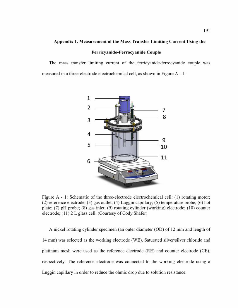
191
Appendix 1. Measurement of the Mass Transfer Limiting Current Using the
Ferricyanide-Ferrocyanide Couple
The mass transfer limiting current of the ferricyanide-ferrocyanide couple was
measured in a three-electrode electrochemical cell, as shown in Figure A - 1.
Figure A - 1: Schematic of the three-electrode electrochemical cell: (1) rotating motor; (2) reference electrode; (3) gas outlet; (4) Luggin capillary; (5) temperature probe; (6) hot plate; (7) pH probe; (8) gas inlet; (9) rotating cylinder (working) electrode; (10) counter electrode; (11) 2 L glass cell. (Courtesy of Cody Shafer)
A nickel rotating cylinder specimen (an outer diameter (OD) of 12 mm and length of
14 mm) was selected as the working electrode (WE). Saturated silver/silver chloride and
platinum mesh were used as the reference electrode (RE) and counter electrode (CE),
respectively. The reference electrode was connected to the working electrode using a
Luggin capillary in order to reduce the ohmic drop due to solution resistance.
192
Before each test, an aqueous solution consisting of 0.01 M K4[Fe(CN)6] /
K3[Fe(CN)6] and 2 M NaOH1 was prepared in the glass cell, and was deaerated by
continuously purging with nitrogen gas. In addition, the solution was kept in the dark to
eliminate the decomposition of ferricyanide and ferrocyanide2.
For each rotating speed, potentiodynamic polarization (PDP) measurements were
conducted, with a potential polarization range from -1.6 V to + 0.4 V (vs. open circuit
potential). Clear and reproducible limiting currents were observed for both anodic and
cathodic polarizations (see Figure 2-8). These limiting current values were later used to
calculate the mass transfer coefficient under each flow condition.
1 K.D. Efird, Flow accelerated corrosion testing basics, in: NACE International CORROSION 2006 conference, 2006, paper no. 06689.
2 M. Eisenberg, C.W. Tobias, C.R. Wilke, Ionic mass transfer and concentration polarization at rotating electrodes, J. Electrochem. Soc. 101 (1954) 306–320.
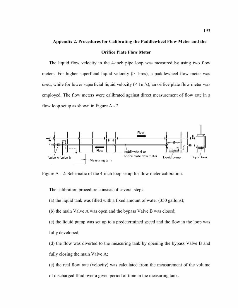
193
Appendix 2. Procedures for Calibrating the Paddlewheel Flow Meter and the
Orifice Plate Flow Meter
The liquid flow velocity in the 4-inch pipe loop was measured by using two flow
meters. For higher superficial liquid velocity (> 1m/s), a paddlewheel flow meter was
used; while for lower superficial liquid velocity (< 1m/s), an orifice plate flow meter was
employed. The flow meters were calibrated against direct measurement of flow rate in a
flow loop setup as shown in Figure A - 2.
Figure A - 2: Schematic of the 4-inch loop setup for flow meter calibration.
The calibration procedure consists of several steps:
(a) the liquid tank was filled with a fixed amount of water (350 gallons);
(b) the main Valve A was open and the bypass Valve B was closed;
(c) the liquid pump was set up to a predetermined speed and the flow in the loop was
fully developed;
(d) the flow was diverted to the measuring tank by opening the bypass Valve B and
fully closing the main Valve A;
(e) the real flow rate (velocity) was calculated from the measurement of the volume
of discharged fluid over a given period of time in the measuring tank.

194
(f) the meter reading and the real flow rate for the given pump speed were
documented; and step (a)-(f) were repeated at various pump speeds.
(g) the calibration coefficient was determined.
For paddlewheel flow meter, the meter reading should be linear with the real flow
rate. By conducting direct flow rate measurements at several pump speeds, the calibration
coefficient for the flow meter can be determined.
For the orifice plate flow meter, the pressure drop across the orifice is measured and
correlated to the flow rate through Bernoulli's principle, as given by:
𝑣𝑠 = 𝐴0𝑈0 = 𝐴𝑝𝑈𝑝 = 𝐶0𝐴0√2𝛥𝑝
𝜌 (A 1)
where 𝑣𝑠 is the volumetric flow rate (m3/s); 𝐴0 is the cross-sectional area of the orifice
hole; 𝑈0 is the flow velocity at the orifice hole (m/s); 𝐴𝑝 is the cross-sectional area of the
pipe; 𝑈𝑝 is the pipe flow velocity (m/s); 𝐶0 is the orifice coefficient; 𝛥𝑝 is the pressure
drop across the orifice (Pa); and 𝜌 is the liquid density (kg/m3). The relationship between
the measured pressure drop and the pipe flow velocity may be rewritten as:
𝑈𝑝2 = 𝐶0
′∆𝑝 (A 2)
where 𝐶0′ is a calibration coefficient. 𝐶0
′ can be determined by conducting pressure drop
and real flow rate measurements at several pump speeds, which is illustrated by an
example, as shown in Figure A - 3.
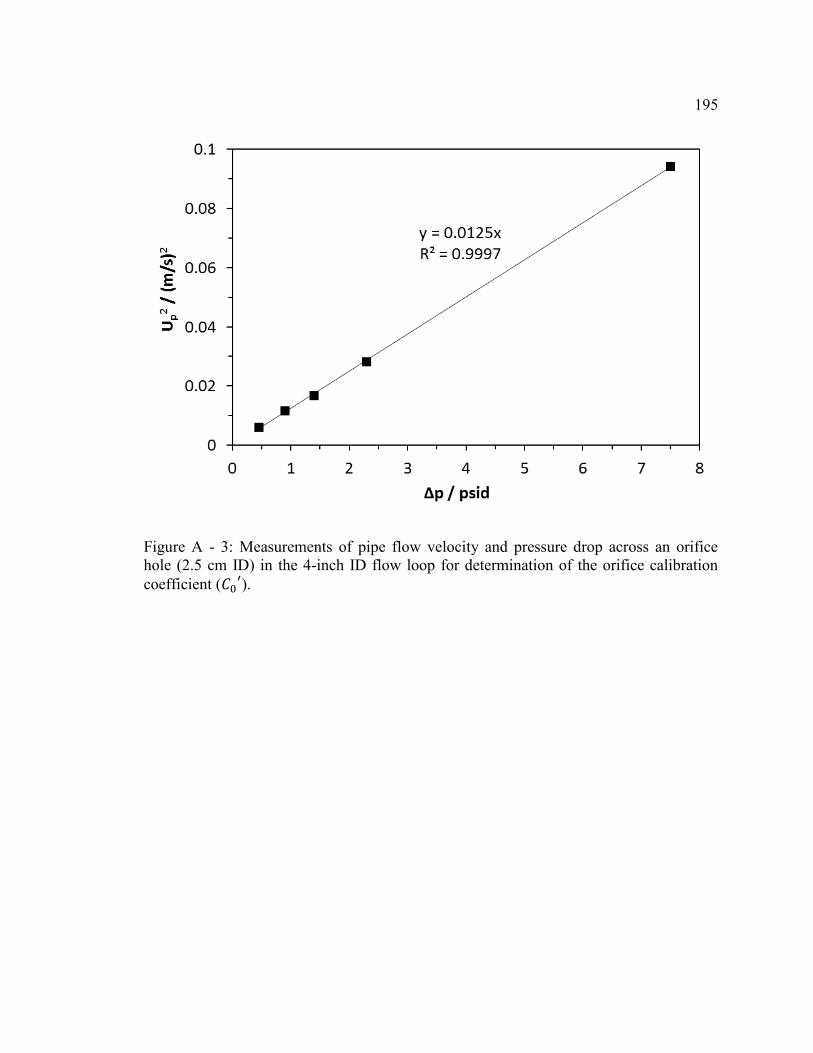
195
Figure A - 3: Measurements of pipe flow velocity and pressure drop across an orifice hole (2.5 cm ID) in the 4-inch ID flow loop for determination of the orifice calibration coefficient (𝐶0
′).
196
Appendix 3. Calculation of Corrosion Rate by Weight Loss and Linear
Polarization Resistance
In this study, weight loss and linear polarization resistance (LPR) measurements were
used to determine the corrosion rates. Corrosion rate (CR) is defined as the metal loss in
thickness per year:
𝐶𝑅 =𝑚
𝜌𝑆𝑡 (A 3)
where 𝑚 is the metal loss; 𝜌 is the metal density; 𝑆 is the surface area of the metal; and 𝑡
is the elapsed time. The measured weight losses can be directly used to calculate the
time-averaged corrosion rate but with no indication of momentary corrosion rate changes.
To measure the instantaneous corrosion rate, LPR was used. LPR is a non-destructive
technique for online corrosion rate monitoring and is capable of capturing the transients
in a corrosion system, for example, such as the addition of an inhibitor. LPR measures the
polarization resistance of the electrode (𝑅𝑝), and is correlated to the corrosion current
(𝐼𝑐𝑜𝑟𝑟) by the Stern-Geary equation:
𝐼𝑐𝑜𝑟𝑟 =𝐵
𝑅𝑝 (A 4)
where B is the proportionality constant, B value (V).
The corrosion current can be used to calculate the metal loss due to the corrosion
reaction from Faraday's law of electrolysis1, as given by:
1 D.A. Jones, Principles and Prevention of Corrosion, 2nd ed., Prentice Hall, Upper Saddle River, NJ, 1996.
197
𝑚 =𝐼𝑐𝑜𝑟𝑟𝑀𝑡
𝑛𝐹 (A 5)
where 𝑀 is the molecular weight of the metal; 𝑡 is the elapsed time; 𝑛 is the number of
electrons involved in the corrosion reaction; and 𝐹 is the Faraday’s constant. Substituting
Equation (A 5) into Equation (A 3), the corrosion rate is calculated as:
𝐶𝑅 =𝐼𝑐𝑜𝑟𝑟𝑀
𝑛𝐹𝜌𝑆 (A 6)
For corrosion of steel (iron), the relationship between the corrosion current and the
corrosion rate can be written as:
𝐶𝑅 = 1.16 ∙𝐼𝑐𝑜𝑟𝑟
𝑆 (A 7)
where the units for CR, Icorr and S are mm/yr, A and m2, respectively. In order to
calculate the corrosion current and the corrosion rate from LPR measurement, a proper B
value needs to be assigned, as shown in Equation (A 4). The B value is defined as: 1
𝐵 =𝑏𝑎𝑏𝑐
ln 10 (𝑏𝑎 + 𝑏𝑐) (A 8)
where 𝑏𝑎 and 𝑏𝑐 are anodic and cathodic Tafel parameters (mV/decade). The Tafel
parameters can be predetermined or measured by the slopes in the potentiodynamic
curves (E-log(i) curves), namely Tafel slopes.
1 R.G. Kelly, J.R. Scully, D.W. Shoesmith, R.G. Buchheit, Electrochemical Techniques in Corrosion Science and Engineering, Marcel Dekker, Inc., New York, NY, 2003.
198
Appendix 4. Calculation of the Absolute Pressure at the Inlet of the CFD
Simulation for Protrusion in the Thin Channel Flow Cell
In Chapter 6, the hydrodynamic conditions surrounding the protrusion specimen were
simulated by using CFD method. A large pressure decrease was found at the leading edge
of the protrusion, as compared to the CFD inlet (see Figure 6-27). However, the CFD
results only showed the relative pressure changes with respect to an arbitrary CFD inlet
pressure. To evaluate the absolute pressure at the protrusion, the true pressure at the CFD
inlet was needed, which required physical pressure measurements in the thin channel
flow cell.
Pressure drop measurements between various pressure taps along the TCFC (“P1, P2,
P3, P4, P5 and P6” in Figure A - 4) were conducted by using a differential pressure
transducer. At the testing flow velocity of 16 m/s, the pressure drop results are given in
Table A - 1. In addition, the pressure in the water tank was monitored by a pressure
gauge.
Due to the computational cost, the CFD simulation only calculated the flow field
10 cm upstream and downstream of the protrusion. The relative positions of the CFD
domain and the physical geometry of TCFC are shown in Figure A - 4. With the pressure
drop measurements and the relative positions, the CFD inlet is calculated to be 40.5 psi
(2.80 bar) smaller than that at location P1. The pressure drop between location P1 and P6
is 78.6 psi (5.42 bar). Considering the fact that the pipe length between location P6 and
the water tank is approximately 160 cm and the tank pressure was measured to be
14.5 psi (1.00 bar), the actual pressure at P6 is calculated to be 1.56 bar, assuming that
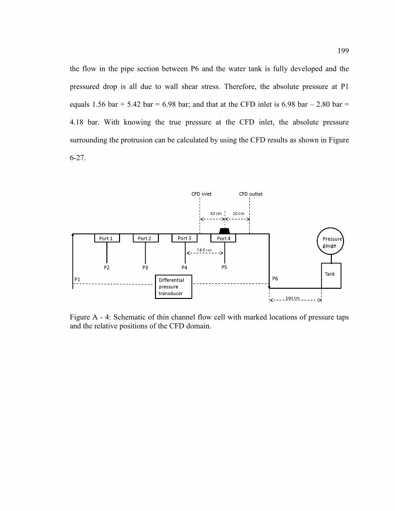
199
the flow in the pipe section between P6 and the water tank is fully developed and the
pressured drop is all due to wall shear stress. Therefore, the absolute pressure at P1
equals 1.56 bar + 5.42 bar = 6.98 bar; and that at the CFD inlet is 6.98 bar – 2.80 bar =
4.18 bar. With knowing the true pressure at the CFD inlet, the absolute pressure
surrounding the protrusion can be calculated by using the CFD results as shown in Figure
6-27.
Figure A - 4: Schematic of thin channel flow cell with marked locations of pressure taps and the relative positions of the CFD domain.
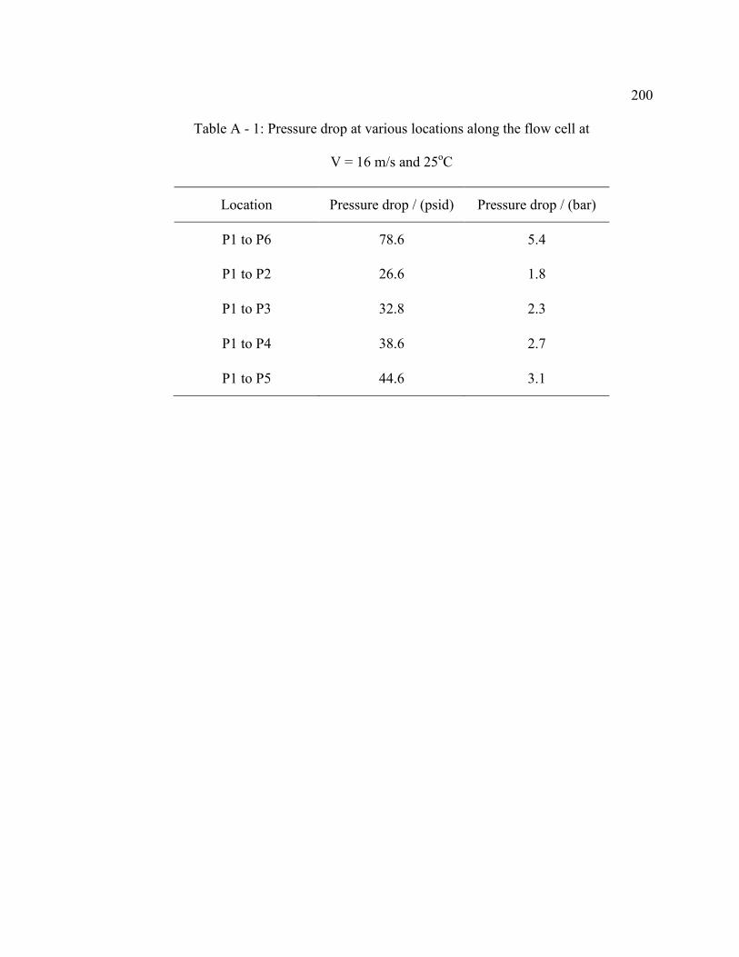
200
Table A - 1: Pressure drop at various locations along the flow cell at
V = 16 m/s and 25oC
Location Pressure drop / (psid) Pressure drop / (bar)
P1 to P6 78.6 5.4
P1 to P2 26.6 1.8
P1 to P3 32.8 2.3
P1 to P4 38.6 2.7
P1 to P5 44.6 3.1

!!!!!!!!!!!!!!!!!!!!!!!!!!!!!!!!!!!!!!!
!!
Thesis and Dissertation Services