Evan H. CoplandATI Allvac, Monroe, North Carolina

Nathan S. JacobsonGlenn Research Center, Cleveland, Ohio

Measuring Thermodynamic Properties of Metals and Alloys With Knudsen Effusion Mass Spectrometry

NASA/TP—2010-216795

November 2010

https://ntrs.nasa.gov/search.jsp?R=20110001597 2018-09-01T01:33:34+00:00Z

NASA STI Program . . . in Profi le

Since its founding, NASA has been dedicated to the advancement of aeronautics and space science. The NASA Scientifi c and Technical Information (STI) program plays a key part in helping NASA maintain this important role.

The NASA STI Program operates under the auspices of the Agency Chief Information Offi cer. It collects, organizes, provides for archiving, and disseminates NASA’s STI. The NASA STI program provides access to the NASA Aeronautics and Space Database and its public interface, the NASA Technical Reports Server, thus providing one of the largest collections of aeronautical and space science STI in the world. Results are published in both non-NASA channels and by NASA in the NASA STI Report Series, which includes the following report types: • TECHNICAL PUBLICATION. Reports of

completed research or a major signifi cant phase of research that present the results of NASA programs and include extensive data or theoretical analysis. Includes compilations of signifi cant scientifi c and technical data and information deemed to be of continuing reference value. NASA counterpart of peer-reviewed formal professional papers but has less stringent limitations on manuscript length and extent of graphic presentations.

• TECHNICAL MEMORANDUM. Scientifi c

and technical fi ndings that are preliminary or of specialized interest, e.g., quick release reports, working papers, and bibliographies that contain minimal annotation. Does not contain extensive analysis.

• CONTRACTOR REPORT. Scientifi c and

technical fi ndings by NASA-sponsored contractors and grantees.

• CONFERENCE PUBLICATION. Collected papers from scientifi c and technical conferences, symposia, seminars, or other meetings sponsored or cosponsored by NASA.

• SPECIAL PUBLICATION. Scientifi c,

technical, or historical information from NASA programs, projects, and missions, often concerned with subjects having substantial public interest.

• TECHNICAL TRANSLATION. English-

language translations of foreign scientifi c and technical material pertinent to NASA’s mission.

Specialized services also include creating custom thesauri, building customized databases, organizing and publishing research results.

For more information about the NASA STI program, see the following:

• Access the NASA STI program home page at http://www.sti.nasa.gov

• E-mail your question via the Internet to help@

sti.nasa.gov • Fax your question to the NASA STI Help Desk

at 443–757–5803 • Telephone the NASA STI Help Desk at 443–757–5802 • Write to:

NASA Center for AeroSpace Information (CASI) 7115 Standard Drive Hanover, MD 21076–1320

Evan H. CoplandATI Allvac, Monroe, North Carolina

Nathan S. JacobsonGlenn Research Center, Cleveland, Ohio

Measuring Thermodynamic Properties of Metals and Alloys With Knudsen Effusion Mass Spectrometry

NASA/TP—2010-216795

November 2010

National Aeronautics andSpace Administration

Glenn Research CenterCleveland, Ohio 44135

Acknowledgments

Helpful discussions about multiple-cell sampling with Christian Chatillon are very much appreciated. We are grateful to Gerd Rosenblatt and Andrea Ciccioli for their critical reviews of this manuscript.

Available from

NASA Center for Aerospace Information7115 Standard DriveHanover, MD 21076–1320

National Technical Information Service5301 Shawnee Road

Alexandria, VA 22312

Available electronically at http://gltrs.grc.nasa.gov

This work was sponsored by the Fundamental Aeronautics Program at the NASA Glenn Research Center.

Level of Review: This material has been technically reviewed by expert reviewer(s).

NASA/TP—2010-216795 iii

Contents

Summary........................................................................................................................................................................ 1 Introduction ................................................................................................................................................................... 1 Knudsen-Cell Vapor Sources and Molecular Beams .................................................................................................... 3

Description of Knudsen Cells From the Kinetic Theory of Gases ......................................................................... 3 Design of Knudsen Cells ........................................................................................................................................ 6 Heating System/Furnace Design ............................................................................................................................ 7 Temperature Measurement ..................................................................................................................................... 8 Thermocouples ....................................................................................................................................................... 8 Pyrometry ............................................................................................................................................................... 9 Molecular Beams .................................................................................................................................................. 10

Mass Spectrometric Analysis of the Molecular Beam ................................................................................................. 12 Instrument Description ......................................................................................................................................... 12 Ionizer ................................................................................................................................................................... 12 Mass Analyzer ...................................................................................................................................................... 14 Detector ................................................................................................................................................................ 15 Vacuum System and Separation of Signals From Background Gases .................................................................. 16 Derivation of the KEMS Equation ....................................................................................................................... 16

Measurement of Thermodynamic Properties of Metals and Alloys ............................................................................ 18 Single-Cell Techniques for Pure Materials ........................................................................................................... 18 Activity Measurements ......................................................................................................................................... 19 Single-Cell Techniques for Alloys ....................................................................................................................... 20 Multiple-Cell Techniques—Direct Measurement of Activities ............................................................................ 22 Activity Calculation for Species That Cannot Be Measured Directly .................................................................. 24

Checks for Correct Operation and Consistency in Measurements .............................................................................. 25 Consistency in Ion Intensity Measurements ......................................................................................................... 25 Consistency in Vapor Sampling and Temperature Measurement ........................................................................ 25 Accuracy of Absolute Temperature Measurement .............................................................................................. 26 Geometry Factor Ratio ......................................................................................................................................... 26 Isothermal Effusion Cells ..................................................................................................................................... 26 Importance of Constant Electron Energy ............................................................................................................. 26

Measurement Procedures ............................................................................................................................................. 26 Sample Exchange ................................................................................................................................................. 27 Instrument Setup and Configuration ..................................................................................................................... 27 Taking Measurements .......................................................................................................................................... 27

Future Directions ......................................................................................................................................................... 28 Summary and Conclusions .......................................................................................................................................... 29 Appendix A.—Symbols ............................................................................................................................................... 31 Appendix B.—SIMION 8 Model of the Ion Source and Analyzer .............................................................................. 33 Appendix C.—Instrument-Control and Data-Acquisition System .............................................................................. 39 References ................................................................................................................................................................... 43

NASA/TP—2010-216795 iv

NASA/TP—2010-216795 1

Measuring Thermodynamic Properties of Metals and Alloys With Knudsen Effusion Mass Spectrometry

Evan H. Copland

ATI Allvac Monroe, North Carolina 28111

Nathan S. Jacobson

National Aeronautics and Space Administration Glenn Research Center Cleveland, Ohio 44135

Summary

This report reviews Knudsen effusion mass spectrometry (KEMS) as it relates to thermodynamic measurements of metals and alloys. First, general aspects are reviewed, with emphasis on the Knudsen-cell vapor source and molecular beam formation, and mass spectrometry issues germane to this type of instrument are discussed briefly. The relationship between the vapor pressure inside the effusion cell and the measured ion intensity is the key to KEMS and is derived in detail. Then common methods used to determine thermo-dynamic quantities with KEMS are discussed. Enthalpies of vaporization vap∆ o

TH —the fundamental measurement—are determined from the variation of relative partial pressure with temperature using the second-law method or by calculating a free energy of formation and subtracting the entropy contribu-tion using the third-law method. For single-cell KEMS instruments, vap∆ o

TH measurements can be used to determine the partial Gibbs free energy if the sensitivity factor remains constant over multiple experiments. The ion-current ratio method and dimer-monomer method are also viable in some systems. For a multiple-cell KEMS instrument, vap∆ o

TH and activities are obtained by direct comparison with a suitable component reference state or a secondary standard. Internal checks for correct instrument operation and general procedural guidelines also are discussed. Finally, general comments are made about future directions in measuring alloy thermo-dynamics with KEMS.

Introduction Accurate measurements of thermodynamic properties in

metal and alloy systems are an important part of metallurgy. These measurements are essential for understanding multiple-component solution behavior and making accurate predictions of the stability of a given system under a range of environ-ments. Furthermore, advanced composites contain many interfaces (e.g., the fiber/matrix interface), and accurate prediction of potential interface reactions requires accurate thermodynamic data (Ref. 1). In recent years, there have been dramatic advances in computational thermodynamics, both

from a fundamental basis and from a phenomenological basis (Ref. 2), but over the same period we have seen a decline in experimental thermodynamics. Basic experimentally deter-mined thermodynamic data are still necessary, both to check the fundamentals-based calculations and as an input to the phenomenological calculations. The need for accurate thermo-dynamic data is recognized by a number of groups that have focused on improving the capabilities of the Knudsen effusion mass spectrometry (KEMS) technique to provide routine measurement of relative partial pressure and partial Gibbs energy in alloy systems (Refs. 3 to 5).

The KEMS technique allows the measurement of relative partial pressure of components, which then is used as a means to obtain thermodynamic property data in condensed alloy systems. The advantage of KEMS is that it can be applied to a wide range of technically important alloy systems over rele-vant temperature ranges. A concise description of the tech-nique is given in the following paragraphs.

A metal or alloy sample is placed in a small enclosure with a well-defined orifice known as a Knudsen cell, or effusion cell, as shown in Figure 1 (Ref. 6). Through careful considera-tion of the inner shape of the cell, effusion orifice, and surface area of the metallic sample, near equilibrium conditions are attained between the condensed phases and the vapor phase while the orifice continuously samples the vapor by effusion. The distribution of the effusing vapor is defined by the shape of the orifice, and typically only a small solid-angle of the distribution is selected to form a molecule beam that is ana-lyzed with a mass spectrometer. A critical, but often over-looked, issue is correctly defining the thermodynamic system that is actually measured (Refs. 7 and 8). In a Knudsen cell, the boundary of the thermodynamic system is the inner surface of the cell, and thus the alloy sample, cell material, and vapor are all part of the equilibrium state being measured (alloy + cell material + vapor). All additional components and phases introduced by the “container” need to be included in the subsequent analysis and in the use of measured data (the same is true for all experimental thermodynamic measurements made in the past and to be made in the future). In addition to components and phases, the temperature and chemical compo-sition of the system need to be determined. Temperature is a particularly critical measurement in thermodynamics and will be discussed in detail.

NASA/TP—2010-216795 2

Figure 1.—Knudsen cell showing key features;

p, partial pressure.

Mass spectrometric analysis of a molecular beam selected from the effusate distribution coming from a Knudsen cell provides information about the identity of the vapor species in the cell and their flux in the beam by analysis of a representa-tive ion beam. If one assumes that a gaseous species A forms an ion A+, the relationship between its partial pressure pA in the effusion cell and the measured intensity in the ion beam IA and absolute temperature T is given by

= AA

A

I TpS

(1)

where SA is the sensitivity factor, which is derived from the instrument configuration and the ionization process. Ideally, absolute pressures can be measured if SA is accurately known. In practice this is extremely difficult; it is typical to assume that SA is constant and to consider relative partial pressures (i.e., pA ∝ IAT). The variation of IAT with inverse temperature leads to the enthalpy of vaporization vap∆ o

TH , which is a cen-tral measurement in KEMS. Partial Gibbs free energy or com-ponent activities are obtained by comparing the pressure of a component in equilibrium with an alloy to that in equilibrium with the pure component at the same temperature (Refs. 8 to 10). The KEMS technique is well-suited for measuring thermodynamic activity. With a single-cell vapor source, thermodynamic activity measurements require mul-tiple experiments where SA must remain constant, whereas with a multiple-cell-configured vapor source, activity is meas-ured directly from the ion intensity ratio from samples in adjacent cells. Thus thermodynamic activity is determined by Equation (2):

= =A A

A o oA A

p Iap I

(2)

Here oAp and o

AI are the partial pressure and ion intensity over the pure component, respectively.

Component activity is a direct measure of the slope of the Gibbs energy surfaces of the stable phases from the direction of the component reference state. The variation of the loga-rithm of activity with inverse temperature gives the partial molar enthalpy and entropy of mixing of the alloy component A, using the second-law method. A well-defined reference state that can be routinely measured is critical for activity measurements. In addition to these thermodynamic quantities, phase transformation temperatures can be determined from changes in the slopes of these plots. The extraction of the various thermodynamic properties from KEMS measurements is discussed later.

KEMS has a long history. It was first applied in 1948 (Ref. 11) and was used quite extensively in the 1960s and 1970s to study the vapors above pure compounds. There are a number of excellent reviews on this technique (Refs. 12 to 18). More recently some groups have extended this tech-nique to multiple-component solutions, as discussed in the review by Kato (Ref. 3). Today there are only a small number of groups worldwide that utilize KEMS for both pure com-pound and solution thermodynamics.

This report discusses the application of KEMS to measure thermodynamic properties in alloy systems. The first part of the report describes each part of a typical magnetic- sector KEMS instrument (Modified Nuclide/MAAS/PATCO 12–90–HT, shown in Fig. 2), with particular emphasis given to the Knudsen-cell vapor source, cell heating, temperature measurement, and molecular beam formation. Although a magnetic-sector mass spectrometer is the best choice for a KEMS measurement, other types of mass spectrometers have been shown to be suitable. The key equation relating the vapor pressure inside the Knudsen cell to ion intensity measured by the mass spectrometer (Eq. (1)) is derived together with a discussion of important features of the ion source design.

Actual measurements are discussed with examples of how to extract meaningful thermodynamic data from the collected data. The critical issue is maintaining constant instrument sensitivity. For a single-cell-configured instrument, constant instrument sensitivity requires a very stable ion source. With-out this instrument stability, special procedures must be utilized such as the ion-current ratio technique or monomer-dimer method in a single-cell configuration or an internal standard in a multiple-cell configuration. Each of these approaches is discussed. Then various routine checks for proper system operation are discussed. We conclude with some comments on future directions of KEMS for alloy thermodynamics. Additional information is provided in the appendixes to aid the reader. Appendix A defines the symbols used in the report, Appendix B provides additional informa-tion about the SIMION Version 8.0 (Scientific Instrument Services, Inc.) model of the ion source, and Appendix C provides a detailed description of the instrument-control and data-acquisition system.

NASA/TP—2010-216795 3

Figure 2.—Knudsen effusion mass spectrometer—magnetic-sector instrument with key components indicated.

Knudsen-Cell Vapor Sources and Molecular Beams Description of Knudsen Cells From the Kinetic Theory of Gases

Figure 1 illustrates a typical Knudsen cell. The Knudsen cell provides a way to probe the vapor in equilibrium with the condensed sample of interest plus cell material. Under the low-pressure conditions used (<10−4 bar) the fugacities of real gases are equal to their partial pressure, and the behavior of the vapor phase is readily described by the kinetic theory of gases. There are several excellent texts on this subject (Refs. 19 and 20). The key relationship derived from kinetic theory to this technique is the Hertz-Knudsen-Langmuir (HKL) expression, which relates the flux of a molecular species striking a surface, JA (mol ⋅ area−1 ⋅ s−1), to its equili-brium vapor pressure in a closed container:

4 2 R

= = π

EA A AE

AA

pN cJV M T

(3)

Here AN V is the density of molecules in the gas, Ac is the average molecular speed, MA is the molecular weight, T is the

absolute temperature, and R is the gas constant. Under equili-brium conditions, the flux of molecular species striking and condensing on a surface is equal to the number of molecular species vaporizing and also relates to equilibrium vapor pressure. In the case where not all molecular species striking a surface condense, Equation (3) is extended to a condensed phase vaporizing into a vacuum (Ref. 21):

2 Rα

= α =π

Eov AEo

A v AA

pJ J

M T (4a)

Here αov is the vacuum vaporization coefficient, which ac-

counts for the reduction in the observed vaporization flux relative to the maximum flux calculated for equilibrium conditions, E

Ap . In the general case where the condensed phase vaporizes in an unsaturated vapor phase, where pA is less than E

Ap , the flux is given by

( )2 R

α −=

π

Ev AA

AA

p pJ

M T (4b)

This is the general form of the HKL equation. Vaporization coefficients vary from ~10−6 to 1, depending

on the material system and molecular species (Ref. 22).

NASA/TP—2010-216795 4

Condensation coefficients may be similarly defined as part of the equilibrium vaporization-condensation process between a vapor and a condensed phase. Vaporization and condensation coefficients are important for ceramics, but for metals these coefficients are generally 1. Therefore in this report we use the HKL equation in the form of Equation (3).

Now consider a vaporizing phase in the Knudsen cell in Figure 1. In the cell, molecule-sample, molecule-wall, and molecule-molecule collisions are important. According to kinetic theory, after a molecule strikes a surface, it desorbs in a completely random direction—that is, the cosine distribution—

( ) ( )d ( ) dcos( ) 2 cos sin d4

θ ω = θ = θ θ θ π Tj N Nc cJ V V

(5)

Here dj(θ) is the element of flux at an angle θ from the normal, JT is the incident flux upon the surface, dω is an element of solid angle ω, as shown in Figure 3(a), and dθ is an element of angle θ.

A plot of dj(θ)/JT versus θ in three dimensions yields a sphere, as shown in Figure 3(b). The HKL equation and flux distribution described by kinetic theory relate directly to the effusion process, which is most simply described as the loss of material from a cell due to the absence of a wall (i.e., the orifice). The type of flow through the orifice of the Knudsen cell defines the maximum pressure and temperature at which the KEMS technique can be applied. If the probability of molecule-molecule collisions is low over the nominal dimen-sions of the orifice, then the flow is characterized as “molecu-lar flow” or “effusion” and the Knudsen cell accurately samples the equilibrium vapor. If the probability of molecule-molecule collisions is high, then the flow is “hydrodynamic” and the Knudsen cell does not accurately sample the vapor phase. The general criterion for effusion flow through an orifice is a Knudsen number, Kn, greater than 8; where Kn = / 2λ r and where λ and r are the mean free path and radius of the orifice. Knudsen numbers from 0.4 to 8 introduce a ~2.5-percent difference between calculated and measured fluxes, which can extend the range of the technique (Ref. 17). The mean free path is the average distance between molecule-molecule collisions and is defined as

( ) 2

12 R

λ =π

P T d

(6)

where P is the total pressure and d is the molecular diameter. At P = 10−4 bar, d = 4×10−10 m, and T = 1273 K, the mean free path is 2.4×10−4 m. Thus, a 1-mm-diameter orifice in a Knudsen cell will accurately sample pressures up to 10−4 bar. Molecular flow is also important because it ensures that the vapor in equilibrium with the condensed phases inside the Knudsen cell does not react via molecule-molecule interactions in the orifice as it exits the cell or in the ensuing molecular beam.

Again, the flux of molecules leaving the orifice is described by the HKL equation. For a real orifice, Equation (3) is modified by including the cross-sectional area of the orifice C and the shape, or Clausing factor, WC, which is the escaping flux from the orifice normalized to the incident flux integrated over the hemisphere. The rate of molar loss of a vapor species is given by Equation (7), which is used to relate measured ion intensity to the corresponding vapor pressure (where t is time).

d ord 2 R 2 R

= =π π

A C A C AA

A A

N CW p W pjt M T M T

(7)

The shape of a real orifice has a more complex effect than just reducing the transmission probability of effusion mol-ecules as represented by WC in Equation (7). Any orifice with a finite length changes the angular distribution of the effusing molecules according to the cosine law. This deviation from ideal behavior can be described analytically or modeled using a Monte Carlo simulation. The pioneering work in the field of Knudsen effusion used the analytical approach (Refs. 23 to 27). The relatively simple behavior of molecular flow through an effusion orifice is easily modeled with a Monte Carlo simulation (Refs. 28 to 30). A simple code can easily be written, and simulations can be conducted with millions of molecules for adequate statistics (Ref. 31, unpublished work). These simulations accurately model Knudsen effusion through an orifice or a small channel.

Monte Carlo modeling of Knudsen effusion easily yields a number of important results. The transmission coefficient, or Clausing factor, can be calculated as the number of escapes divided by the number of molecules entering the orifice. This is shown in Table I. The major advantage of the Monte Carlo approach over analytical approaches is that the number of wall collisions can be counted and averaged. Some of the molecules will go through the channel with no wall collisions. This frac-tion can also be readily obtained with the Monte Carlo simula-tion. As the length of the channel increases, the probability that molecules will pass through the orifice without any wall colli-sions decreases. These results are all listed in Table I. An understanding of this wall collision behavior is important in understanding Knudsen effusion because the molecule would be expected to thermally equilibrate with the wall after a collision.

In addition, the angle to the normal through the channel can be recorded for each molecule. A simple sorting routine then gives the angular distribution emerging from an orifice. A polar plot of dj(θ)/JT is shown in Figure 3(c) for a very thin orifice and a channel. Note that the channel gives a more directed distribution. The same results are obtained from the analytical approach (Ref. 27). It is important to note that these Clausing factors are all calculated. The degree of agreement with the actual experiment depends on the accuracy of machining and measuring the actual orifice dimensions and attaining molecular flow conditions.

NASA/TP—2010-216795 5

Figure 3.—Molecules desorbing from a surface or emerging from an orifice.

(a) Molecule desorbing from a surface into a solid-angle element; θ, angle to the normal from a surface; dω, element of solid angle ω. (b) Cosine distribu-tion for a molecule desorbing from a surface. (c) Distribution for a thin orifice and a channel, derived from a Monte Carlo simulation.

TABLE I.—CLAUSING FACTORS FOR DIFFERENT ORIFICES FROM MONTE CARLO MODELING Length/radius,

l/r Clausing

factor Average number of wall

collisions for returns Average number of wall

collisions for escapes Fraction of escapes with no

wall collisions 0.1 0.9523 1.0513 0.0523 0.9048 1.0 .6720 1.5870 .7136 .3821 2.0 .5144 2.2429 1.7694 .1718 4.0 .3566 3.5742 4.7624 .0557

10.0 .1910 7.5607 20.3455 .0098

NASA/TP—2010-216795 6

The Clausing factor and the distribution of effusing molecules have important ramifications for the accuracy of vapor sampling, the design of the vapor source furnace, and molecular beam formation. In some cases, an orifice with a high Clausing factor is desirable, whereas in other cases a cell with a lower Clausing factor is desirable. A short, or “knife-edge,” orifice has a Clausing factor close to unity and, thus, a near-uniform flux distribution. This orifice also yields the minimum number of wall collisions within the orifice and a large vapor flux. This type of orifice has traditionally been used with the Knudsen effusion weight-loss technique. One disadvantage of this type of orifice is that a large fraction of the effusing molecules are trapped inside the furnace heat shields, which can act as a coaxial “virtual effusion cell” and contaminate the effusate coming from the effusion cell. Also the high rate of material loss attained with a large knife-edge orifice can produce errors in vapor-pressure sampling. The last major problem with knife-edge orifices is that they promote surface diffusion (Ref. 16). Longer, or channel, effusion orifices have a lower Clausing factor and a lower probability of molecules leaving the cell, particularly at high angles from the normal, but there is a higher probability that the effusing molecules will have collided with the orifice wall. The lower Clausing factor helps in attaining solid/vapor equilibrium and accurate sampling of the vapor phase. Low Clausing factors at high angles from the normal greatly reduce the amount of effusate trapped in the furnace and contaminating the molecular beam. Careful selection of the effusate distribution close to the normal and within the orifice to form the molecular beam, limits the sampling of molecules that have collided with the orifice wall. From the authors’ perspective, channel orifices are ideal for the KEMS technique.

Design of Knudsen Cells The considerations discussed thus far can be used to design a

cell for optimum vapor sampling. A real cell is not a closed container, and removal of vapor means the sampled flux is not the same as that passing through an imaginary plane near the surface of the sample in a closed container. The presence of the orifice means that there is no condensation/revaporization flux in the area taken by the orifice. Thus, pressure in this region is necessar-ily lower than in the rest of the cell. Furthermore, not all con-densed phases have vaporization and condensation coefficients equal to 1. Thus, the measured vapor pressure must differ from the equilibrium value.

This problem has been approached by several investigators (Refs. 15 and 32 to 35). In general, the closest approach to equilibrium is attained with the following conditions:

(1) A large sample surface-area to orifice-area ratio, which ensures that many more molecules are involved in vaporization and condensation than escape from the ori-fice (ratio values of greater than 100 are recommended (Ref. 16)).

(2) A large Clausing factor for vapor transport from the sam-ple surface to the orifice.

(3) A low Clausing factor for the cell orifice (as discussed in the previous section).

(4) Materials being measured have vaporization and conden-sation coefficients that are close to unity (e.g., metals).

These factors are summarized in the Whitman-Motzfeld equa-

tion (Refs. 32 and 33):

1 11 2

= + + − α C

e mv D

W Cp pD W (8)

Here pe is the equilibrium pressure inside the Knudsen cell, pm is the measured vapor pressure, WC is the Clausing factor for the orifice, C is the surface area of the orifice, D is the surface area of the bottom of the cell cavity, αv is the vaporization coefficient, and WD is the Clausing factor for the cell itself. A number of assumptions have been made in this derivation, most notably that the condensation coefficient equals the vaporization coefficient. However, the important points about the design of a Knudsen cell are captured in the basic Whitman-Motzfeld equation. Our cells have a cavity with a diameter of 10 mm and height of 7.6 mm, and a typical orifice has a diameter of 1.5 mm and a length of 4.0 mm. If tabulated Clausing factors (Ref. 27) and a vaporiza-tion coefficient of 1 are assumed, the ratio Pe/Pm has a value of 1.005.

The selection of an appropriate material for a Knudsen cell is a challenging problem. No combinations of materials are truly inert, considering solubility and reactivity at high temperatures. Selection of an appropriate material requires examining all possible reactions and solution formation possibilities with phase diagrams and thermodynamic calculations. Table II presents some typical cell materials for different types of samples. Typi-cally, ceramics are used for metals and refractory metals are used for ceramics. Often it is best to select a cell material made of a stable compound in the system under investigation. For example, SiC in a graphite cell can be used to study carbon-saturated SiC (Ref. 36), Si3N4 can be used to study Si-O-N compounds (Ref. 37), and Al in an alumina cell can be used to study Al-saturated Al2O3 (Refs. 38 and 39).

TABLE II.—KNUDSEN-CELL MATERIALS

Material studied Knudsen-cell material Reference SiC-C Graphite Rocabois et al. (Ref. 36) Si3N4 Si3N4 Rocabois et al. (Ref. 37) Al-Al2O3 Al2O3 Copland (Refs. 38 and 39) ZrO2-Y2O3 W Stolyarova and Semenov; Belov and Semenov (Refs. 18 and 40) SiO2 Ta with ZrO2 liners Zmbov et al. (Ref. 41) TiC, ZrC, HfC, ThC W, Ta with graphite liners Kohl and Stearns (Ref. 42) Ti-Al alloys Y2O3 Eckert et al. (Ref. 43)

NASA/TP—2010-216795 7

Heating System/Furnace Design Resistance heating or electron bombardment is typically

used to heat the Knudsen cells. Both heating methods have their advantages and disadvantages. Below about 1000 °C, resistance heating needs to be used, whereas at higher temper-atures either resistance heating or electron bombardment can be used. Resistance heating has the advantage that no arcing or ion formation takes place inside the furnace. A simple passive control system is used and generally voltage is regulated. Thus, temperature is set by a voltage. However, this control system makes temperature sensitive to any changes in resis-tance in the circuit, and great care needs to be taken when designing all electrical connections and feed-throughs. An issue closely related to resistance heating is that power is proportional to current squared and that high currents are necessary, which means the large-diameter water-cooled power feed-throughs are required. Furthermore, heating cannot be directed to only the cell, so the entire area around the cell needs to be heated, resulting in more power usage. It is generally impractical to heat the cell in a multiple-zone furnace, and extra care must be taken to avoid ther-mal gradients.

The electron-bombardment heating method allows direct heating of the cell alone, and it is relatively easy to apply two or more zones to remove thermal gradients. However, the circuitry is more complex than that used for resistance heating. Also, the higher voltages of electron bombardment can lead to arcing and interference with spectrometer electronics.

In the authors’ KEMS instrument, resistance heating is used. Heating elements are made of either W or Ta and are illustrated as part of the entire flange assembly in Figures 4 and 5. Ta elements can easily be formed at room temperature, and they heat to temperatures just slightly lower than W elements. The “hairpin” design used with the single-cell flange (Fig. 4) provides uniform heating and allows sighting of side blackbody holes for pyrometer temperature measurements. A 25-µm-thick sheet heating element made from either W or Ta is used in the multiple-cell flange (Fig. 5) and provides the most uniform heating.

The furnace must provide an isothermal hot zone large enough to contain the effusion cell(s): thermal gradients within the Knudsen cell cannot be tolerated (Ref. 44). In most laboratory applications, long tube furnaces are used and provide a uniform heat zone in the center. This is not possible with KEMS. The furnace must be compact to allow placement of the Knudsen cell(s) as close to the ionizer as possible. An isothermal hot zone in such a compact furnace is achieved with a carefully constructed multiple-layer heat-shield pack that completely surrounds the cell, with a small opening for the molecular beam. The heat shields act as a “virtual black-body” cavity around the Knudsen cell(s) and ensure uniform heating. In addition, the Knudsen cell can be placed inside a conductive envelope or block to further reduce thermal gra-dients. The use of a conductive envelope (shown in Fig. 5) is

vital for a multiple-effusion-cell vapor source. At temperatures below 900 °C, heat transfer by radiation becomes less effi-cient, and other ways to maintain isothermal conditions need to be considered. Placing the effusion cell inside a heat pipe envelope is an option (Ref. 45).

Figure 4.—Single-cell flange used in our system. Resistance

heating is used with the “hairpin” element.

NASA/TP—2010-216795 8

Figure 5.—Multiple-cell flange used in our system with resistance heating using a sheet

element. The x-y position motors are computer controlled. Temperatures are meas-ured with a pyrometer from the bottom.

As noted, the cavity created by the heat shields produces a

“virtual Knudsen cell.” Although most of the vapor escapes through the hole in the heat shields, some of it remains in this cavity for a short time. This problem is rarely discussed, but these trapped vapor species would be expected to collide with the inner heat shield and cell block, eventually escaping from the hole in the heat shields. Thus, these species constitute a secondary vapor flux that is not representative of the cell interior. The secondary flux cannot be eliminated completely, but it may be minimized by placing the cell orifice as close to the heat shields as possible.

Temperature Measurement The importance of precise temperature measurement rela-

tive to thermodynamic temperature in experimental thermo-dynamic measurements cannot be overstated. Perhaps the most difficult challenges with regard to the determination of heats of vaporization and other thermodynamic properties arise from errors in measuring the absolute temperature of the effusion cell. The best approach to measuring absolute tem-perature is to use the techniques and standards that define or realize the International Temperature Scale (ITS–90, Refs. 46 to 50) and to calibrate the measuring instrument directly in situ with one or more fixed points. This approach ensures that

the measuring instrument is as close as possible to the absolute temperature scale and removes the costly and time-consuming procedure of routine calibration at a national standards labora-tory. The KEMS technique is ideally suited for in situ calibra-tion because “pure” metals can be placed inside an effusion cell and continuously ramped through the invariant point solid + liquid + vapor + container while both the signal from the temperature sensor and relative partial pressures in the equilibrium vapor are monitored (Ref. 51). The fixed points of Ag (1234.93 K), Au (1337.33 K), and Cu (1357.77 K) are the most practical and, together with the Planck radiation law ratio, define ITS–90 above 1234.93 K.

The temperature of the cell must be uniform, and the meas-uring device must accurately reflect the temperature within the cell. Two methods are commonly used for measuring temperatures—thermocouples and pyrometry. In alloy studies, pyrometry is the more reliable technique, but at temperatures below about 800 °C, the use of thermocouples is necessary. In both cases it is critical to measure the temperature as close to the cell as possible.

Thermocouples Although thermocouples are generally seen as easy to set

up and use for temperature measurement, particular care must

NASA/TP—2010-216795 9

be taken to ensure that accurate values are obtained (Ref. 52). The major challenges encountered when using thermocouples with KEMS are the quality of the junctions, incorrect use of lead wires (the uninterrupted thermocouple wire must extend all the way from the hot junction to the ice-point reference), use of an ice-point reference, prevention of contamination inside the furnace, and routine calibration. The basic thermo-couple equation is

1 2 1 2( )− = α − J JV V T T (9)

Here V1 – V2 is the measured potential difference, 1J is the reference junction and 1JT is its temperature, 2J is the measuring junction and 2JT is its temperature, and α is the Seebeck coefficient. The reference junction should be in a controlled 0 °C ice-point reference, thus the measured voltage directly indicates the temperature of 2J .

The junctions may be formed with a variety of methods, including an oxyacetylene flame and spot welding. The choice of method depends on the oxidation resistance of the particu-lar type of thermocouple wire used. Typically the actual thermocouple wires are made of high-purity, reference-grade material. Wires with compositional variations may generate secondary voltages and produce erroneous readings.

Although Pt/Pt-Rh thermocouples are widely used for high-temperature studies, we have found a number of critical problems that effectively preclude their use with KEMS alloy studies. The first is contamination of the wires. This is particu-larly a problem for Pt/Pt-Rh thermocouples, which are not recommended for use in vacuum systems and environments containing metal vapors, as encountered in a KEMS alloy study. Pt readily alloys with metals such as Al and Ag, form-ing intermetallic compounds. A partial solution is to use a ceramic thermocouple sheath to protect the thermocouple wires as much as possible. Frequent calibration and replace-ment of contaminated thermocouple wire is essential, but this is very time consuming and expensive. Calibration can be performed by comparison to a National Institute of Standards and Technology (NIST)-traceable standard thermocouple, but fixed routing in the effusion-cell vapor-source furnace makes this impossible. A further factor acting against the use of thermocouples in KEMS studies is that they are not a primary measurement technique used to define and maintain ITS–90. This introduces unnecessary calibration steps and the potential for uncertainty in measuring absolute temperature.

Pyrometry When the temperatures of interest are in a suitable range,

pyrometry is the best technique for measuring the temperature of the Knudsen-cell vapor sources in KEMS instruments. Some of the major advantages are that it is a noncontact technique, with the pyrometer placed outside the furnace and vacuum chamber. Also, one pyrometer can be used to measure temperature at multiple locations, which improves the consis-

tency of calibration. The key advantage is that pyrometry, as stated in the “Temperature Measurement” section, is based on the Planck radiation law, which in ratio form defines ITS–90 at all temperatures above the Ag fixed point (1234.93 K). Thus, pyrometry is the standard method for realizing thermo-dynamic temperature through the use of Equation (10):

90 2 90

90 2 90

( ) exp(c ( )) 1( ( )) exp(c ) 1λ

λ

λ −=

λ −L T T X

L T X T (10)

where Lλ(T90) and Lλ(T90(X)) are the radiances of a blackbody at wavelength λ, at the temperature to be determined T90 and the fixed point T90(X), where X can equally be Ag (1234.93 K), Au (1337.3 K), or Cu (1357.77 K) and where the second radiation constant c2 = 0.014388 mK (Ref. 46).

To ensure the correct application of pyrometry, one must take care to design and fabricate blackbody radiation sources in the effusion cell to have an emissivity that approaches unity. Typically, this means that the length-to-radius ratio of the cavity should be at least 10:1. There are a number of similarities in constructing a close-to-ideal blackbody cavity and an effusion cell that accurately samples the equilibrium vapor. When functioning correctly, a blackbody should emit a uniform flux of radiation; and when visually observed at steady-state conditions, it should never appear darker than the surrounding parts of the furnace. If the blackbody source does appear darker, it is likely due to reflected radiation from hotter surfaces like the heating element. If this occurs, radiation shields are needed to prevent radiation from the hotter surface from directly impinging on the blackbody source.

The pyrometer also needs to be carefully aligned with the blackbody sighting holes and chamber window so that there are no obstructions. An instrument that allows sighting through the optics of the pyrometer is invaluable and allows the experimenter to see the source area of the measurement exactly and to confirm that the proper object is being sighted. Furthermore, it is important for the source area to lie fully within the opening of the blackbody and for the measured temperature to be independent of the location of the source area inside the blackbody.

After the blackbody cavities, the next critical issue is the window transmissivity changing with time. Even with a well-designed vapor source to minimize the trapping of effusing vapors, with proper placement of the blackbody source, and with the use of shutters; there will inevitably be some conden-sation of high-temperature vapors on the window. As a result, the window needs to be cleaned regularly, and the transmis-sivity of the window needs to be measured. Window changes can be checked routinely using an in situ calibration technique where “pure” Ag, Au, or Cu are placed in an effusion cell and the invariant point solid + liquid + vapor + container is ramped through while both temperature and relative partial pressures are monitored. This procedure can be done a number of times during an experiment. Figure 6 illustrates an example of this for Au in a graphite container (Ref. 51). A clear plateau

NASA/TP—2010-216795 10

Figure 6.—Melting point of Au in a graphite cell, showing variation of the measured

ion intensity and temperature with time. The plateau on the measured ion intensity curve shows the existence of an invariant, or triple point.

is observed in relative pAu, which is characteristic of an invariant reaction. The changes in slope of the curve in a temperature-versus-time plot correspond to the start and finish of melting. Because the thermal mass of the sample is small in comparison to the whole furnace and the blackbody is not fully inside the metal sample, the measured temperature is not fixed while the invariant equilibrium exists. Thus, the invar-iant can only be observed on heat-up, and the first thermal arrest is the invariant temperature. The slower the heating rate, the more accurate that these measurements are. The measured current from the photomultiplier at the invariant point is used to determine the window transmissivity for correcting the measured temperature.

Traditionally disappearing filament pyrometers have been used, but these are subjective, with measurements varying from operator to operator, and are no longer used. Today, there are a variety of pyrometers available that use a photo-multiplier tube to measure radiance at a given wavelength; these have been shown to work very successfully. It is com-monly thought that the effusion orifice and cell can be used as a blackbody cavity for temperature measurement. Indeed, this is cited as an advantage of a cross-axis ionizer, as illustrated in Figure 2. However, in practice this involves sighting through the apertures in the ionizer, and alignment becomes difficult. The major problem with sighting the orifice is contamination of the window above the orifice with time. In general, the authors have found that precise temperature measurements are better made from a side or bottom port, as close to the cell as possible.

Molecular Beams In KEMS only a small portion of the total distribution of

the molecules effusing from the cell orifice form the molecular

beam that is analyzed by the ion-source/mass spectrometer. Thus, the portion of the distribution that is selected is critical to the success of KEMS in general, but it is particularly important for a multiple-effusion-cell-configured KEMS instrument. In the traditional approach, the effusion orifice and the larger diameter entrance orifice or slit to the ion source are considered to define the molecular beam. However, as shown in Figure 7(a), molecules can enter the ion source from a wide angular range (defined by holes in the heat shields and ion source entrance). Clearly this situation allows molecules to enter the molecular beam that do not originate from inside the effusion cell and will result in erroneous results. A technique developed by Chatillon and coworkers (Refs. 5, 45, and 53) can be used to solve this problem. Two small, fixed apertures are introduced between the effusion cell and ion source, as shown in the restricted collimation part of Figures 7(a) and (b). These apertures select a small, well-defined angular range that a molecule must be traveling to enter the ion source, form an ionization volume, and thus be analyzed. The selected angular range is fixed and independent of the vapor source. For the vapor effusing from a Knudsen cell to be sampled, the center of the orifice needs to be moved to be concentric with the fixed apertures. The beam molecules must now have velocities aligned along the axis perpendicular to the orifice and minimal molecule-molecule interactions within the beam. Thus the beam will accurately represent the vapor above the condensed phase in the Knudsen cell. Although a well-defined molecular beam is essential for Knudsen-cell mass spectrom-etry (Ref. 53), it has not been given adequate attention in the past. Our system uses two apertures above the Knudsen cell to define the beam (see Figs. 1 and 7). Following Morland et al. (Ref. 53), we refer to the fixed aperture closest to the cell as the “field aperture” and the aperture closest to the ion source as the “source aperture.”

NASA/TP—2010-216795 11

Figure 7.—Molecular beam collimation. (a) Ray diagram showing that a small field aperture limits the sampling area and allows only

the material effusing from the cell to be sampled (adapted from Ref. 53). (b) Three-dimensional diagram of molecular beam for-mation and collimation, showing the beam-defining orifices, ion-beam formation, and a well-defined ionization volume.

A well-defined molecular beam strictly defines the source

area and angular range of molecules and restricts the amount of background vapor that reaches the ionizer. Furthermore, by using a small field aperture one can make the source area of the molecular beam smaller than the cross-sectional area of the cell orifice. This definition of the beam effectively removes the effect of the shape of the orifice on the flux distribution of the molecular beam and makes KEMS measurements inde-pendent of orifice shape. This effect is analogous to the requirements of sampling the radiation from fully within the blackbody when temperature is measured with a pyrometer.

The major advantage of defining the molecular beam this way is calibration. Consider two Knudsen cells on a multiple-

cell flange—one with a pure material that has a known vapor pressure and one with an alloy with a component that has an unknown vapor pressure. Ideally we can use the cell with the pure material to determine the calibration constant that relates measured ion intensity to vapor pressure. However, this deter-mination of a calibration constant only gives a reliable value if the molecular beam from each cell is sampled in exactly the same way.

Our goal in this section is to describe the molecular beam mathematically. We need to understand how the intensity varies a function of the pressure in the cell, the Clausing factor of the cell orifice, the distance from the cell orifice, the area of the cell orifice, and the placement of defining apertures in the

NASA/TP—2010-216795 12

molecular beam. Chatillon and his group (Refs. 5, 45, and 53) discuss defining a molecular beam in the KEMS technique, and we shall follow their arguments.

Molecular beams are analogous to the transmission of light—a stream of photons. Many of the equations developed for light are readily applicable to these molecular beams. First, note that the flux decays as 1/a2, where a is the distance from the source to the receiver. The basic equations for the flux received from a radiating element are derived in the paper and textbook by Walsh (Refs. 54 and 55). The problem germane to the collimation of a molecular beam in a mass spectrometer is the transmission of the beam from one disk source to another coaxial disk source. The fraction of molecules that leave the radiating disk and arrive at the receiving disk is given by

2 2 2 2 2 22 21 2 1 2 1 2

1 2 21

( ) ( ) 4( , , )

2+ + − + + −

=r r a r r a r r

F r r ar

(11)

Here a is the distance between the two disks, r1 is the radius of the radiating disk, and r2 is radius of the receiving disk. This quantity is the unit of the solid angle that reaches the second aperture (Ref. 53). Thus, the flux reaching the second aperture can be described as

( )1 2( ) , ,

2 R

′θ= π

C AA

A

W pj F r r aM T

(12)

Here WC(θ´) is the Clausing factor discussed earlier in Equation (7), but it is for the limited angle from the normal θ´ defined by the field and source apertures (Eq. (13)). Note also that the number distribution is not the same everywhere in the molecular beam. This is evident if a portion of the beam distribution is sampled as shown in Figure 3(c). If the center of the collimating apertures is collinear with the center of the distribution, then there is a symmetric number density about this center.

10

( ) , d′θ

′θ = θ ω ∫ C

LW Tr

(13)

The function T is the angular distribution of a real orifice relative to an ideal cosine distribution, as discussed previ-ously. We select the function for the smaller angles about the normal to the orifice. Equation (13) then describes the flux reaching the ionization chamber in terms of the critical beam-defining parameters. Figure 7(b) shows the fixed apertures that select a portion of the effusate distribution to form a molecular beam. In our system the molecular beam includes the solid angle about 0.76° from the normal, and the furnace is trans-lated on an x-y plane to ensure that all cells that are sampled form the same angle to the normal. Such variations from cell-to-cell in the multiple-cell system are accounted for in the experimentally determined geometry factor ratio (GFR), as

discussed later in the “Derivation of the KEMS Equation” section.

Mass Spectrometric Analysis of the Molecular Beam

Although the quantitative nature of the KEMS technique was indicated in the introduction, it is important to reiterate it at the start of a discussion of the ion source, mass analysis, and detector. The aim of this technique is to measure the relative partial pressure of vapor species in equilibrium with a condensed sample as a function of sample composition and absolute temperature. The pressure of each species is meas-ured indirectly by sampling its flux in a molecular beam by ionization and analysis of the ion beam. Ideally, the ion-beam composition is representative of the molecular beam; however, the indirect nature of these measurements introduces a range of factors that affect the measured intensities in the mass spectra. These factors are unrelated to sample composition and temperature. Clearly then, the goal is to reduce the effect and variation of these other factors to allow the accurate study of vapor pressure with temperature and sample composition. The next section briefly discusses the aspects of mass spectrometry with the aim of identifying the other factors and indicating how their effects can be reduced to provide accurate meas-urement of thermodynamic activities.

Instrument Description All mass spectrometers consist of four common elements:

(1) the ion source, (2) the mass analyzer, (3) the detector, and (4) the vacuum system (Ref. 56). Quadrupole, time-of-flight, and magnetic-sector instruments have all been used success-fully to obtain thermodynamic data from metallic and alloy systems. It is important that the instrument introduce no mass-discrimination effects or that corrections be applied for these effects. Thus, in general, magnetic-sector instruments are preferred because they can be designed to minimize mass discrimination.

Ionizer The purpose of the ion source is to produce ions representa-

tive of the sample and to accelerate and focus them through a static potential field to form a well-defined ion beam that is directed to the mass analyzer. The vapor is introduced to the ion source as a well-defined molecular beam that is selected from the material effusing out of a Knudsen-cell vapor source. There are a variety of methods available for producing ions from gases (thermal ionization, vacuum discharge, ion impact, photo ionization, and electron impact), all of which have advantages for specific applications. Electron impact is the most versatile for high-temperature inorganic vapors and is generally used. The main advantages offered by electron impact are good sensitivity, ease of forming a controlled

NASA/TP—2010-216795 13

electron beam, and the ability to vary the energy of the elec-trons over a wide range.

Ion sources used for KEMS have either (1) a mutually per-pendicular arrangement of molecular, electron, and ion beams or (2) parallel molecular and ion beams with a perpendicular electron beam. As shown in Figures 1 and 7(b), our mass spectrometer has a mutually perpendicular arrangement. Although this arrangement may reduce sensitivity, it has the advantages that collisions between ions and neutral molecules are reduced following ionization and that the kinetic energy spread of the molecules (due to the temperature of the vapor source) is not transferred to the ionization process and to the ion beam. This arrangement results in a smaller energy spread in the ion beam, which results in better ion-beam focusing and resolu-tion in the mass analyzer. In a static electric field, ions with the same starting location, direction, and kinetic energy per unit charge will traverse an identical path (i.e., no mass discrimina-tion) (Refs. 56 and 57).

Understanding ionization processes is important for interpret-ing measured mass spectra because it provides a method to identify possible “parent molecule(s)” for each ion species. The identification process typically involves determining the relative ionization potential (IP)/appearance potential (AP) of each parent and fragment ion and studying the shape of their ioniza-tion efficiency (IE) curves. This information allows the selec-tion of an electron energy that will ensure that the measured ion intensity is not, in part, due to a fragmentation process, while providing the maximum instrument sensitivity. Electron impact ionization, ionization-efficiency curves, and ionization cross sections have been discussed in detail by many investigators (Refs. 14, 56, 58, and 59). Therefore, only the basic aspects of the ionization process important to activity measurements are summarized here.

An electron with kinetic energy E collides inelastically with a neutral atom or molecule, some kinetic energy is absorbed, and the valance electron configuration of that atom takes an excited state. Above a threshold energy Ec, the collision results in the removal of a valance electron and the formation of a stable ion. The energy for this process is the IP.

( ) ( ) 2− + −+ → +A g e A g e (14)

Simple ionization of a molecule may also occur:

( ) ( ) 2− + −+ → +AB g e AB g e (15)

where B represents another alloy component. However, many other processes may occur besides these simple ionization processes. Fragmentation may occur:

( ) ( ) ( ) 2− + −+ → + +AB g e A g B g e (16)

Double ionization and ion-neutral molecule reactions may also occur. An understanding of the ionization process is important

for correlating the correct magnitude of ion intensity with partial pressure in Equation (1).

One important tool in understanding ionization processes of high-temperature inorganic vapors is an IE curve or a plot of the energy of the ionizing electrons versus ion current. Drowart and Goldfinger (Ref. 13) and Grimley (Ref. 14) discuss the use of IE curves to understand fragmentation patterns. Figure 8 is a typical IE curve. The most common type of informa-tion obtained from such curves is the AP shown in the figure. The AP for the ionization of the molecule AB is composed of

AP IP= + + ΣAB AB ABD E (17)

Here DAB is the dissociation energy of AB, and ΣE is the sum of any excitation levels of the molecule.

In the case of an atomic species, there is, of course, no dis-sociation term. Generally, one of two methods is used to obtain the AP—the linear extrapolation (LE) or the critical slope (CS) method. The LE method involves fitting a straight line to the apparently linear section of the IE curve, extrapolating back to the electron energy axis, and taking the intercept as the AP. This method is subjective, since a series of data points are approx-imated by the operator to be linear. Fundamentally, the IE curve is never linear (Ref. 60). The CS method is based on assigning the initial curvature of the IE at the IP to a Maxwellian energy distribution of the thermally emitted electrons (Refs. 56 and 58).

It should be noted that this is an approximation, since the energy distribution of thermally emitted electrons shows devia-tions from a pure Maxwellian distribution (Refs. 61 and 62). A plot of the logarithm of ion intensity versus electron energy exhibits a linear region below the AP. The slope of the linear region is typically independent of material. The point where this curve deviates from linearity is the IP for the ion. The CS method is generally considered to be more reliable than the LE method (Ref. 58). APs are generally instrument specific (Ref. 56) because of the spread of electron energies and the method of calculation. A stable and known electron energy across multiple experiments is critical in thermodynamic measurements because it ensures a consistent IE for each species. Figure 8 is a representative IE curve with the LE method used to obtain an AP for Al. To select a consistent operating electron energy, it is essential to measure IE curves as part of each experiment in a thermodynamic study and to set the electron energy relative to the measured APs.

The probability of ionization by electron impact is put into a quantitative context through the concept of ionization cross section. An ionization cross section, σA(E) (dimensions × area/molecule), is specific to an ionization reaction (e.g.,

( ) ( ) 2− + −+ → +A g e A g e ). It is defined experimentally by the following relation (Ref. 58):

( ) ( ) ( )

( )( )

( )

e e AA

AA

e e A

II E I E l E

II EE

I E l

+ −

+

−

= ρσ

σ =ρ

(18)

NASA/TP—2010-216795 14

Figure 8.—Example of an ionization efficiency (IE) curve showing the appearance poten-

tial (AP) derived from the linear extrapolation (LE) method, where the coefficient of determination, R2, is 0.9634 and AP is 6.83 eV.

where ( )+

AII E is the ion current of the ion immediately after ionization and before extraction, ( )−

eI E is the current of impacting electrons, ρA is the density of the vapor in the ion source, and le is the “collision path” of the electrons through the vapor in dimensions of length. An identical definition of cross section is used for molecular species. When multiple ionization processes occur, a total cross section of the neutral species is defined as the summation of all ion species collected in the ion current (Ref. 59). Although the cross-section concept is simple, the determination of accurate absolute values from experi-ments involves considerable difficulties. This description implies the following necessary conditions:

( )+AII E Ions are only produced by single-electron impact

in the electron beam, and the fraction of ions col-lected to ions produced is known.

( )−eI E There is a total current collection of electrons

producing ions, a uniform electron current (or known distribution if inhomogeneous), and no collection of secondary electrons.

le The electron trajectory and the shape of the ioni-zation volume is accurately known, and therefore the collision path of the impacting electrons is known.

ρA The vapor density is uniform and known in the ionization region. Typically for molecular beams this involves knowing the temperature and pres-sure of the vapor source, the velocity of the molecules, the total beam flux, and a known dis-tribution, if inhomogeneous.

The ionization cross section is a central quantity in the sen-sitivity factor in Equation (1). Difficulties in obtaining relia-ble, absolute cross sections result in the use of calculated atomic cross sections (Refs. 63 to 66) together with the addi-tive rule for molecules species for absolute pressure calcula-tions with KEMS. More recently, better experimental results have been published for absolute cross sections and for cross-section ratios for various species (Refs. 67 to 77), but there are still many molecular species with no data, and there is little agreement between reported values of commonly studied species (Ref. 17). The problem is clear for atoms, and it is even greater for molecules. For molecules, the atomic cross sections are commonly summed and then multiplied by 0.75 (Ref. 4). This method for molecules is an estimate, and errors are up to 30 percent or more. These problems suggest that the best approach for KEMS is to use measured cross-section ratios (made with the specific instrument), and this is best achieved with a well-designed multiple-cell configuration. Improved calculations also lead to more reliable cross sections (Ref. 66).

Mass Analyzer The resulting ion beam is sorted according to its mass-to-

charge ratio by the mass analyzer. Mass spectrometers are generally classified according to the mass analysis method—magnetic-sector, quadrupole, or time-of-flight. Our instrument is a 90° magnetic-sector instrument that uses the force exerted on a moving charged particle in a magnetic field to separate the beam according to ion momentum. For the conditions of equal kinetic energy and charge, these momentum spectra become mass-to-charge spectra. The key equation is then

NASA/TP—2010-216795 15

2 2

2=

m r Bq V

(19)

Here m is the mass of the ion, q is the charge, r is the radius of deflection, B is the magnetic field, and V is the accelerating voltage. Thus the mass-to-charge ratio varies as the square of the magnetic field and the inverse of the voltage. Generally, spectra are scanned by varying the magnetic field. However, finer scanning may be accomplished by varying the voltage.

Magnetic-sector instruments are generally preferred for high-temperature vapor studies because of their lack of mass-discrimination effects. The identity of an ion species is deter-mined from the mass-to-charge ratio, whereas its relative abundance is determined from the intensity of its peak in the mass spectrum. The isotopic “fingerprint” is also useful in identifying peaks. Tables and computer codes are available to calculate isotopic abundances to check these values. The analyzer must sort the ions so that adjacent mass numbers are sufficiently separated. The resolution Res of an instrument is defined for two adjacent masses, M and M + ∆M (Ref. 56), in Equation (20):

Res =∆MM

(20)

The units of M and ∆M can be mass units, voltage, or mag-netic field units. If the desired distance between the peaks is taken as the base width, then the distance between the peaks becomes 1. However, a 10-percent peak-overlap criterion is typically used. In a magnetic-sector instrument, resolution is set by the beam-defining slits at the exit of the ionizing cham-ber (electrostatic accelerator) and entrance to the multiplier. These are vertical slits whose widths are adjustable from the outside of the instrument. These slits define the beam and resolution (Ref. 56):

RadiusRes(Source slit Detector slit)

≈+

(21)

In our system the radius is 305 mm, the source slit is ~0.25 mm, and the detector slit is ~0.025 mm. Thus, a resolu-tion of ~1100 is calculated. For an inorganic species with a molecular weight of 100, we can separate an adjacent species of 100.1. We have found that this resolution is adequate for at least partial separation of the inorganic vapor species from background hydrocarbons.

Detector The intensity of each mass-to-charge peak is measured by the

detector—generally a Faraday cup or multiplier. Our instrument uses a 22-dynode electron-multiplier detector where the selected ions pass through a defining slit and impinge on the first dynode, producing secondary electrons. These electrons are

then measured with a sensitive electrometer (ion-current meas-urement) or an ion counter (Refs. 56 and 78).

The output of the Faraday cup goes to a precision 2×1011-Ω resistor, and the output of the last dynode in the multiplier goes to a precision 1×109-Ω resistor. The voltage drop VA across the resistor R is measured with an electrometer, and the ion current IA is simply calculated from Ohm’s law:

=

A

AVIR (22)

Ion currents can be converted to counts per second, since 1 ampere equals 6.24×1018 counts per second. Multiplier gains are determined from comparison of the multiplier output to the Faraday cup output. The major disadvantage of ion-current measurements is the dependence of sensitivity on mass num-ber (Ref. 56). This problem of dependence on mass number is introduced in the first, or conversion, dynode, where the number of electrons ejected from a single ion depends on the mass of that ion (Ref. 78). Generally, for masses greater than ~50 amu,

Kγ =A AM (23)

Here γA is the gain, K is a constant, and MA is the mass. To avoid these mass bias effects, we do most of our measure-ments with ion counting. If the system is set up so that >99 percent of the pulses are counted, then the efficiency of the first dynode does not matter and the multiplier introduces no mass-discrimination effects (Ref. 79).

An important aspect of detection efficiency is the “dead time,” τ, of the detector. This is the period of time required by the detector to process an event and is related to the duration of the pulse (Ref. 78). As the count rate increases, the time between events approaches τ and the probability of multiple events occurring during the processing time increases, result-ing in possible errors. Our detector is nonextendable and multiple events occurring during this processing time simply go unnoticed and are lost. To avoid large dead-time effects, one should keep count rates low. However, the need for a large dynamic measurement range makes this difficult, and a correction is thus needed for high count rates. The empirical correction is quite simple with the true count rate RT given by

(1 )

=− τ ⋅

mT

m

RRR

(24)

where Rm is the measured count rate and τ is the dead time. The major factor determining τ is the shape of the pulse leaving the multiplier and how detector electronics modify this shape during amplification prior to counting. It is worth determining if the detector amplifier changes the pulse shape, which can be done with a representative pulse provided by a signal generator and oscilloscope. It is critical to avoid

NASA/TP—2010-216795 16

excessive gain and “clipping” of the amplified pulse, which increases pulse duration and can introduce spurious secondary pulses. A typical multiplier pulse has an amplitude of ~10 mV and is ~5 ns in duration. Provided that the amplified pulse remains less than 20 ns, there is very minimal dead time loss at count rates approaching 5 MHz. If needed, τ can be deter-mined experimentally by measuring the ion intensity of two isotopes over a wide range of count rates. Provided that the isotopic abundance KT is unaffected by the changing experi-mental conditions, the ratio of the measured isotopes is given by Equation (25), from which the dead time can be extracted.

1 1 2

2 2 1(1 )(1 )

− τ ⋅= =

− τ ⋅T m m

TT m m

R R RKR R R

(25)

To ensure good accuracy of this measurement, it is impor-tant to use an element with the largest possible isotopic abundance ratio (i.e., >10).

Vacuum System and Separation of Signals From Background Gases

A reliable, oil-free vacuum system is an essential part of a KEMS system. The location of the pumps on our system are shown in Figure 2. The vacuum system of course allows proper operation of the air-sensitive components such as the ionizer and the detector. An oil-free system minimizes back-ground, which may block the ions formed from the molecular beam. Today’s oil-free turbopumps and backing pumps, together with ion pumps, allow the construction of a true oil-free pumping system throughout.

In addition to minimizing the overall background, ions formed from the species in the cell can be distinguished from any specific background peaks by high resolution in the ion sorter, by the measurement of isotopes, and by use of a “shut-ter profile.” The shutter, which is typically a small paddle with a slot, can be externally scanned across the molecular beam. The shape of the resultant profile gives some information about the origins of the molecular beam (Ref. 13). The inten-sity of the beam is thus taken as the difference between the maximum (peak + background) and the minimum (back-ground). In our system, the precision movement of cells in one direction, in both single- and multiple-cell flanges, together with a small field aperture, allows a shutter profile to be obtained. Alternatively, in the multiple-cell flange, an empty cell can be used for background measurements.

Derivation of the KEMS Equation

The central KEMS equation can be derived now that the Knudsen-cell vapor source and mass spectrometer have been described. This follows directly from the vapor flux in the molecular beam selected from the distribution of material effusing from the Knudsen cell (molecular-beam flux equa-tion) and the definition of the ionization cross section

(Eq. (18)). However, in accordance with the aim of identifying factors that affect the measured ion intensity and that are unrelated to sample temperature and composition, it is useful to rewrite Equation (18) in terms of the number of ions pro-duced per second in the elementary volume dv in the region defined by the intersection of the molecular and electron beams, ( )+

An E (Refs. 71 and 80) (this is prior to the formation of the ion beam):

( )d ( ) ( )d

( ) ( ) d

+ −

−

= ρ σ

= σ

e e A AA

Ae e A

A

n E v I E l E vjI E l E vc

(26)

Here jA is the flux of molecular beam. The region defined by the intersection of the electron and molecular beams is the ionization volume and, provided that the electron beam is wider than the molecular beam, it has an approximately cylindrical shape (Fig. 7(b)).

Consider first an electron beam with a uniform flux. A uni-form electron flux requires a specially designed electron gun (Refs. 81 and 82). Further consider a molecular beam with uniform flux across a plane perpendicular to its direction. As noted, the intensity of the molecular beam decreases with 1/a2, where a is the distance from the cell orifice to the ionization region. Provided that the molecular beam stays fully within the electron beam, this will result in a uniform rate of ion production across the ionization volume.

KEMS typically uses thermally generated electrons, so the electron beam does not have a uniform flux across a plane perpendicular to its direction. Furthermore, the molecular beam is not uniform across a plane perpendicular to its direc-tion, as shown in Figures 3(c) and 7(b). The mathematical description of a molecular beam has been discussed previously with Equation (12). Here the differential of the molecular beam flux can be written as follows:

2( ) 1 d

2 RC A

AAS

W pj saM T

′θ= π ∫ (27)

where ds is an element of a surface perpendicular to the molecular beam. Substitution of Equation (27) into (26) with the assumption of a homogeneous electron beam and inte-grating, results in the total number of ions produced per unit time, ( ) :+

AN E

2

2

( ) ( )d

( ) 1 1( ) d d2 R

( ) 1 ( ) d d8R2 R

+ +

−

−

=

′θ= σ π

′θ π= σ π

∫

∫ ∫

∫ ∫

A AV

C Ae e A

AAV S

C A Ae e A

AV S

N E n E v

W pI l E s va cM T

W p MI l E s va TM T

(28)

NASA/TP—2010-216795 17

Here ( )+AN E is the total number of ions produced per unit time

(ion intensity). The integral in Equation (28) is difficult to evaluate for these reasons:

(1) Coordinate systems—The molecular beam is best described with polar coordinates such that r is meas-ured perpendicular to the beam. As noted, a beam of thermally generated electrons is difficult to describe in any coordinate system. If we assume that the electron beam apertures create a cylindrical electron beam, then the electron beam may be described with polar coor-dinates such that its radius is perpendicular to the direction of the electron beam. These two coordinate systems must be consistent for the integration.

(2) Electron beam—As noted, the mathematical descrip-tion of this is not known.

Nonetheless, the dependency of ion intensity is clearly indi-

cated in Equation (28). The ion intensity is a function of the ionization volume, the electron beam flux, the vapor pressure in the cell, the temperature of the cell, the size of the orifice, the distance from the effusion orifice, and the ionization cross section. We can easily extract the KEMS equation (Eq. (1)) from Equation (28):

2( ) 1( ) ( ) d d

8R2 R

k ( )

+ − ′θ π

= σ π σ

=

∫ ∫ C A Ae e AA

AV S

A A

W p MN E I l E s va TM T

p ET

(29)

Here k is a constant incorporating all the factors in Equation (29).

The final stage in deriving Equation (1) is converting the rate of ion production to the measured ion intensity in the mass spectra. This involves extracting ions from the ion source, forming an ion beam, separating the beam according to mass-to-charge analysis, and measuring intensities. Therefore the measured ion intensity IA(E) depends on the ion-extraction efficiency ε(x, y, z), the transmission probability of the mass analyzer τion, the detection coefficient γA, and the isotopic abundance fA. The ion-extraction efficiency is a nonuniform function of the position in the ion source, which highlights the need for a consistent ionization volume to ensure that the ion beam accurately represents the rate of ion formation. The mutually perpendicular design of the ion source and small ionization volume ensure that the ions have similar starting positions and that their initial velocity in the ion-beam direc-tion is negligible. Therefore, the transition probability should be identical for all ions:

( ) ( ) ( , , )+= ε τ γion A AA AI E N E x y z f (30)

Substitution of Equation (30) into (29) gives the KEMS equation:

k ( )( )( , , )

A AA

ion A A

p EI ET x y z f

σ=

ε τ γ (31)

Commonly, this equation is written in the following form:

k ( )( )

′=

σA

AA

I E Tp

E (32)

where k' is a constant relating ion intensity and temperature to pressure.

Much of this report has focused on our multiple-cell vapor-source flange and the use of an in situ standard. The proper use of a multiple-cell configuration requires that the molecular beam from different cells be sampled in a consistent manner. Consistent sampling is only possible if the shape of the ioniza-tion volume is constant and the same portion of the flux distributions of the molecular and electron beams intersect (i.e., the relative positions of the beams do not change).

Consistent sampling is achieved by introducing two fixed apertures (the field-aperture and the source-aperture) between the Knudsen-cell vapor source and the ion source, as discussed previously. These apertures fully define the shape and position of the molecular beam in the ion source. Also, the apertures limit the trajectory of molecules that can enter the ion source to a small, clearly defined solid angle, which removes the possibility of direct contamination of the molecular beam from adjacent effusion cells, revaporization flux from the shields, and general background. The ionization volume is then fixed by the stability of the potential surface in the ion source, which determines electron beam shape. Part of tuning the ion source, therefore, involves adjusting this potential surface to align the maximum flux portions of the electron and molecular beams. The final aspect is the consistent alignment of the effusion orifice with the fixed apertures so that the same portion of the effusate distribution from each effusion cell is selected by the molecular beam. It is helpful to consider the molecular beam to be independent of the molecular species it samples. Alignment of the cells is very important and is checked visually with a camera sighting the effusion orifice through the molecular beam apertures (Fig. 2) and through scans of ion intensities with cell position.

If the conditions of consistent ionization volume, a fixed electron beam, and consistent alignment of the cell orifice with the molecular beam-defining apertures are met, the integration over the electron beam and the molecular beam shape in Equation (29) will be constant from cell to cell. Provided that the cells are isothermal, for a comparison between different molecular beams, the ion ratio is given by

I

II

( ) ( ) C( ) ( ) C

σ= ⋅ ⋅

σA AA

B BB

I E E pI E E p

(33)

where CI and CII are constants relating only to variations in the flux distribution in the molecular beam because of differences in effusion orifice geometry. Since the true nature of the

NASA/TP—2010-216795 18

electron and molecular beam flux distributions and the exact shape of the ionization volume are not known, absolute measurements cannot be made. However, consistent sampling allows accurate relative measurements. When different species coming from one cell are compared, the GFR for a nonideal effusate distribution is the same for both species and it cancels out.

From this discussion, the effect of orifice shape on the effusate distribution needs to be removed before the relation-ship between vapor pressure and sample composition and temperature can be studied accurately. The calibration of orifices is easily achieved with a multiple-cell configuration by putting the same material in different cells and comparing the rate or ion production at the one temperature. This calibra-tion procedure is referred to as a GFR measurement:

-cell I I

II-cell II

( ) CGFR( ) C

= =A

A

I E

I E (34)

Measurement of Thermodynamic Properties of Metals and Alloys

Single-Cell Techniques for Pure Materials

Most KEMS instruments use a single Knudsen-cell vapor source. A variety of techniques have been developed for

measuring thermodynamic quantities with a single-cell config-uration (Refs. 12 to 17). First consider a pure metal. The determination of the heat of vaporization ∆vapHo(A) is one of the most common measurements in KEMS for

( ) ( )

ApgAsA

=eqK (35)

This is done with two related methods (Ref. 12): the second-law method and the third-law method. The second-law method is based on the van 't Hoff equation:

eq vapd ln K ( )d(1 ) R

oTmH A

T∆

= − (36)

where Keq is the equilibrium constant. As indicated by Equation (32), pA is proportional to IA(E)T. In

most metals it has been found that the primary ionized species is A+ and is representative of the vapor. Thus a plot of ln(IA(E)T) versus 1/T gives a linear plot with slope vap ( ) R∆ o

TmH A ,where Tm is the average temperature of the measurement. Figure 9 is an example of such a plot for Au and Ni.

Equation (36) implies that ∆vapHo(A) is independent of tem-perature, but given that the heat capacities of the condensed and gaseous phases are different, ∆vapHo(A) is temperature dependent. This makes it difficult to compare measured

Figure 9.—Example of Au and Ni heat of vaporization, ∆Hv, measurement; IA, ion

intensity in counts per second from A(g); E, energy of ionizing electrons; and T, absolute temperature.

NASA/TP—2010-216795 19

data taken at different temperatures. It is better to report the enthalpy for the reaction at the standard temperature (298 K), which is done with the Σ´ method (Refs. 51, 83, and 84) using the free-energy functions (FEF298.15) for the condensed and vapor phases, which are known for the pure metals.

298.15 (FEF ) ln( )∆ − − = +AR I T P Q T (37)

where 298.15 298.15FEF ( )= −o oTG H T for each phase. If the left-

hand side of Equation (37) is plotted versus 1/T, the slope (Q) gives ∆vapHo(A) at 298.15 K and the intercept (P) gives an estimate of instrument sensitivity factor for species A (Ref. 51). The third-law method is similar but requires the conversion of the measured ion intensities into absolute vapor pressures:

[ ]298.15 vap 298.15 (FEF ) R ln( ) ( )∆ − − = ∆ oAT p H A (38)

Of course, free-energy functions referenced to zero kelvin can be used to derive a heat at zero. Basically the Gibbs free energy is calculated at a series of data points, and the entropy contribution is subtracted. This results in the heat of vaporiza-tion for each data point. The average is taken from all the data points, and this method can give a very accurate heat-of-vaporization measurement. However, as has been discussed, all the factors necessary to accurately convert ion intensities to vapor absolute pressures are not typically known.

Activity Measurements Thermodynamic activities aA provide a measure of the reac-

tivity of a component (A) in a solution phase, designated here as β, relative to a reference state indicated by the super-script (o). Activities are fundamental to understanding the thermodynamics of multiple-component systems (Refs. 8 to 10). Activity is defined as the ratio of a component’s fugacity (Ref. 8) in the solution to the reference state and also in terms of the change in Gibbs free energy for a mixing or solution reaction, which provides relative chemical potentials,

βµ − µoA A , ( )( ), , ,...

β βµ = ∂ ∂B

AA T P nG N , where NA is the num-

ber of moles of A(g), as shown in Equation (39):

mix AR ln R lnβ β∆ = µ − µ = =oA A A o

fG T T af

(39)

The value of the activity depends on the choice of the refer-ence state. The selection of a reference state is arbitrary, but it must be clearly defined and, ideally, something that can be routinely realized in an experiment (Refs. 9 to 10). A typical experimental reference state is the stable defect-free phase of the pure-element at the temperature of interest (Raoultian reference state). The mixing or solution reactions that represent the activity of components A and B in the binary solution phase AxBy

β are shown in Equations (40a) and (40b)

(Ref. 10). The reference states for pure A and B are the δ-phase and ε-phase, respectively. In these reactions, the amounts of A and B added are so small relative to the amount of AxBy

β that the composition of the solution does not change:

δ β β

1

mix R ln

+

β β

+ =

∆ = µ − µ =

x y x y

oAA A A

A A B A B

G T a (40a)

ε β β1

mix R ln

+

β β

+ =

∆ = µ − µ =

x y x y

oBB B B

B A B A B

G T a (40b)

Each partial mixing reaction is studied directly by compar-ing the vaporization behavior of A from the reference and solution-phase equations (Eqs. (41a) and (41b)). For pure A in the δ-phase, aA = 1 and pA = o

Ap by definition. At high tem-peratures and low pressures, the equilibrium vapor approaches ideal behavior and fugacity can be determined by measuring the partial pressure of a characteristic vapor species. The mixing reaction equation (Eq. (40a)) is obtained by subtracting the vaporization reactions (Eq. (41a) – (41b)), and the activity of component A in AxBy

β is determined directly at T by com-paring pA in equilibrium with the solution and reference state (Eq. (2)).

( )

vapΔ R ln oA

A A g

G T p

δ

δ

=

= − (41a)

( )1

vapΔ R ln

x y x y

AA

A B A B A g

G T p

β β+

β

= +

= − (41b)

A = AoA

pap

(2)

If the composition and activity of all components in a sys-tem are measured, then the total Gibbs energy of mixing can be determined by Equation (42), where xi is the mole fraction. Measuring the partial pressure of all components is not com-mon, but in this case the temperature dependence of the logarithm of activity can be used to determine the partial molar heat of mixing as shown in Equation (43).

mix R lnβ∆ = ∑ i ii

G T x a (42)

( )mixd ln( )

d 1 R

β∆=i iHa

T (43)

where mix iH β∆ is the partial molar heat of mixing. If partial molar heat can be obtained for each of the alloy’s

components, then the integral heat of mixing can be calculated

NASA/TP—2010-216795 20

and compared with that obtained from calorimetric measure-ments or other techniques (Ref. 43).

mix mixβ β∆ = ∆∑ i i

iH x H (44)

Single-Cell Techniques for Alloys Even though thermodynamic activity is a pressure ratio or

relative measurement, a single-cell KEMS instrument can be used if absolute pressures can be determined and the instru-ment sensitivity does not vary from run to run. Constant sensitivities are difficult to achieve because of changes in cell position and the molecular and electron beam alignment in the ionizer, which all lead to changes in the ionization volume. Some investigators have a valve that isolates the ionizer in a highly rigid cell-holding system to minimize this problem (Refs. 85 and 86), but this may not be possible on all instru-ments. Several methods have been developed to overcome the problem of a nonconstant sensitivity factor in a single-cell configuration. The ion-current-ratio technique is widely applied, and several groups are associated with the develop-ment of this technique (Refs. 87 to 89), which is based on the Gibbs-Duhem relationship (Ref. 8). For a binary alloy,

ln ln 0A A B Bx a x a+ = (45a)

d ln d ln d ln

= =

A AA B B

B B

a Ia x xa I

(45b)

1

ln d lnA A

A

x xA

A BBx

Ia xI

=

=

= −

∫ (45c)

1

ln d ln lnA A

A

x xB B

A BA Ax

I xxI x

=

=

γ = − −

∫ (45d)

Here xi is the mole fraction of a component. Equation (45d) is equivalent to Equation (45c), where γA is the activity coeffi-cient of component A, which is given by aA /xA. This change is made because Equation (45d) is readily integrated graphically. Similar to Equation (43), the partial molar heats of mixing are obtained by the temperature dependence of activity or in terms of ion-current ratios as

( )( )mix

1

d lnR d

d 1

A A

A

x xB A

BAx

I IH x

T

=β

=

∆ = −

∫ (46)

It is important to recognize that the ion-current technique requires that measurements are taken at a series of compositions starting from a “pure” component at one side of the system. Some representative measurements from our laboratory on Fe-Al alloys are given in Figure 10 (Ref. 90). This is a very valuable technique and has been used extensively with binary alloys and even some ternary alloys (Refs. 3, 4, 91, and 92).

The ion-current ratio or pressure ratio is a sensitive indica-tor of phase changes. The ratio represents the ratio of the slope

Figure 10.—Example of activity data for the Fe-Al system at 1573 K from

the ion-current ratio method (Ref. 90).

NASA/TP—2010-216795 21

of the Gibbs energy surface from two corners of the system, which can change dramatically as the phase equilibria in the system change (Refs. 3 and 93):

( ) vap vapln CR

∆ − ∆= +

i iB A

A BG G

I IT

(47)

Here vap∆ iAG and vap∆ i

BG are the partial molar free energies of vaporization from a solution i of A and B, respectively, and C is a constant. A linear slope for ln (PA/PB) versus 1/T is obtained for a liquid solution over a narrow temperature range. When the liquidus is reached, crystals of the solid will precipi-tate. The partial molar quantities would change dramatically with composition, and hence the plot would no longer be linear. Such plots for a range of compositions can yield quite accurate solidus and liquidus lines. Nunoue and Kato (Ref. 94) have used this technique with the Fe-Ge system, and Copland has used this technique with the Ni-Al-O system (Ref. 95), as shown in Figures 11(a) and (b). Note the discontinuity in the activity ratios in Figure 11(a), which clearly establish the liquidus lines. The convergence at 1640 °C of five phases (not possible according to the phase rule) indicates the need to look in detail at this region. This convergence is shown in more detail in Figure 11(b), which indicates eutectic and peritectic points over

a small temperature region. This phase change is further con-firmed with the activity ratios of Ni-23Al and Ni-27Al, which show the three-phase field of γ + β + Al2O3 (Fig. 11(c)).

Another technique used to measure activity in alloys with a single-cell KEMS is the dimer-monomer method that was developed by Berkowitz and Chupka (Ref. 96). This requires a system that has a dimer-monomer equilibrium, which is not common:

2A(g) = A2(g) (48)

The equilibrium ratio over the alloy is compared with that over the pure component A, and the activity is given by

2

2

alloy

alloy=oAA

A oA A

I Ia

I I (49)

Here alloyAI and

2

alloyAI are the ion intensities of the monomer

and dimer, respectively, for the alloy, and oAI and

2oAI are the

ion intensities of the monomer and dimer, respectively, for the pure material. In situations where the monomer and dimer are measureable, this is a valuable technique for single-cell systems (Ref. 4).

Figure 11.—Measurement of phase boundaries in the Ni-Al-O system (from

Ref. 95). Copyright Elsevier; used with permission. (a) Measurement of phase boundaries (γ, β, γ', γ' + β) using ion activities. (b) Focus on the region near 1640 °C. (c) Activity ratios of Ni-23Al and Ni-27Al showing phase boundaries.

NASA/TP—2010-216795 22

Figure 11.—Concluded.

Multiple-Cell Techniques—Direct Measurement of Activities

The critical need for a constant sensitivity factor is solved with a multiple-cell-configured KEMS, as shown in Figures 5 and 7(b). Critical conditions for this method are (1) a fixed ionization volume that allows consistent sampling of the

molecular flux from all cells, (2) the ability to consistently sample a well-defined portion of the effusate distribution from each cell, (3) an isothermal furnace that allows sampling from all cells at one temperature, and (4) the ability to accurately measure the absolute temperature of the samples. Once these conditions are achieved, the multiple-cell configuration provides two independent methods for determining component

NASA/TP—2010-216795 23

activities in alloy systems. The most general method is the direct comparison of the measured ion intensities IA of a characteristic species (A) over the alloy and the pure compo-nent (°) at a single temperature (Refs. 5, 13, 97, and 98). The activity of A (aA) is obtained from the following equation:

oII

I

CC

⋅= = ⋅ = ⋅

⋅

oA A AA

A o o oAA A A

Sp I T Iap I T S I

(50)

where SA is the instrument coefficient that has been discussed. Since identical molecular species are compared, all factors associated with the ion-extraction and mass-sorting processes are constant, and provided that the ionization volume remains constant, the instrument coefficient ratio reduces to the differ-ence in effusate distribution due to the variation in the shape of each orifice, which is represented by the GFR: C1/CII (Refs. 5, 13, 17, and 97 to 99). The GFRs are determined for each pair of cells in a separate run. A standard substance is placed in all cells, and provided that the cells are isothermal, the vapor pressures will be identical. This vapor pressure combined with the assumption of a constant ionization volume allows the GFRs to be determined by a comparison of the ion intensities for each pair of cells (Refs. 5, 17, 97, and 98), as discussed previously and described by Equation (34).

This method does not involve the determination of absolute pressures and requires no comparison with tabulated thermo-dynamic data, and therefore gives activities directly. An addi-tional advantage is that the requirement for accurate absolute temperature measurement can be relaxed to some degree because all intensities are measured at a single temperature in an isother-mal block (Ref. 5). Unfortunately, the high reactivity and high vapor pressures of pure components prohibit the use of direct measurements in some systems. The most important example is pure Al for Al-containing alloys. For these cases, a second method of determining activities is required.

The second method of determining activity is an indirect procedure that uses a secondary reference, for which Au(s,l) + graphite is ideal. In this method, activities are determined at each T by comparing the measured ratio, Au

oAp p or Au

oAI I ,

to the accepted vaporization behavior Au o o

Ap p of Au(s,l) + graphite and the pure-element reference, Equation (51):

Au IIAu AuoIAu Au

CC

= ⋅ = ⋅ ⋅ ⋅

o oA i

A o o oiA AT T T T

p pp I Sap p I S p

(51)

The ratio CI/CII is the GFR and accounts for variations in effusion orifices. GFRs are routinely measured to be 1.00 ± 0.01 for a pair of cells with the field and source aper-tures in place (Refs. 100 to 102). The SAu/SA term is an instrument sensitivity (or ionization cross-section) ratio that relates the secondary reference, Au

op of Au(s,l) + graphite, to the pure-element reference, o

Ap . These terms are

determined in a separate experiment comparing the measured ratio of the vaporization behavior of A and the pure-element reference Au

o oAI I of Au(s,l) + graphite, to the accepted

vaporization behavior Au o oAp p . The SAu/SA terms must be

independent of T; thus the accepted vaporization behavior for both must be correct and able to be measured routinely (Refs. 100 to 102).

Au Au AuI

II

CC

o oo

o oA A AT T

I pSS I p

= ⋅ ⋅

(52)

Although it is more complex than the direct method (Eq. (50)), this procedure provides the following advantages: (1) multiple alloys can be measured in a single experiment (depending on the number of effusion cells in the furnace); (2) T measurements are calibrated with the Au melting in each experiment (Tmp(Au) = 1337.33 K is a fixed point defining ITS−90) (Ref. 46); and (3) routine measurements of

( )vap 298.15 Au∆ oH by the second- and third-law methods provide a systematic accuracy check (Refs. 51 and 103). Examples of the successful use of this second indirect method of measuring activities are given for the Ni-Al-O system in Figures 11(a) and (c) and for the Ni-Al-Pt(-O) system in Figure 12 (Refs. 95 and 101). The data in Figure 12 show how maintaining a constant Ni/Al ratio and varying the Pt content affects the activities of Ni and Al (Refs. 100 and 102).

In addition to absolute activities, the multiple-cell KEMS technique allows relative activities to be determined directly by comparing the relative partial pressure of species in equili-brium with different samples, with compositions I and II, and in adjacent effusion cells in a single experiment, according to Equation (53a), where any difference in flux distribution of the molecular beams is again represented by the GFR. Rela-tive activities are the most direct measure of any differences between the solution behavior and phase equilibrium of two samples. According to Equation (39), relative activities provide a direct measure of the difference in chemical poten-tial between the two compositions, as in Equation (53b).

I

IIII

IA

C(I II)C

AA

Ia

I− = ⋅ (53a)

R ln (I II) (I) (II)i iA A AT a − = µ − µ (53b)

This method is particularly powerful for studying phase transformations when the compositions are chosen so that they are on different sides of a single phase. An example of this is shown in Figure 11(c), where the measurement compares Ni-23Al and Ni-27Al, on either side of γ′-Ni3Al, in the γ′ + γ + Al2O3 and γ′ + β + Al2O3 three-phase fields. This result clearly shows that the γ′-Ni3Al phase decomposes prior to melting (Ref. 95).

NASA/TP—2010-216795 24

Figure 12.—Example of activity data for the Ni-Al-Pt system obtained using the

multiple-cell method (adapted from Ref. 100). Activity Calculation for Species That Cannot Be Measured Directly

The preceding discussion was based on the situation where an alloy component vaporizes or sublimates directly to charac-teristic species that can be measured easily. This situation is not the case in some reactive alloy systems because one component may not vaporize directly or its vapor pressure may be too low to measure. However, its activity can be calculated through an additional equilibrium between the components and easily measurable vapor species. Ti-Al-O is an important example of this type of system. Here interstitial O has a very high solubility in Ti-rich compositions, and

O concentrations less than 10 at.% have O partial pressures pO lower than about 10−20 atm at 1500 K. Clearly, these low partial pressures are not measurable by KEMS. Fortunately, both Al(g) and Al2O(g) are present with significant vapor pressures in this highly reducing system, and they are related by the reaction 2Al(g) + O(g) = Al2O(g). This relation is used to calculate the pO in equilibrium with the atomic O in these alloys. The following equilibria can all be studied with a pure-Al(l) + α-Al2O3 standard:

( ) ( )

Al

Al , Al

K o

s l g

p

=

= (54a)

NASA/TP—2010-216795 25

( ) ( ) ( )

2

2 3 2

Al O

4 3Al , 1 3 -Al O Al O

K o

s l s g

p

+ α =

= (54b)

( ) ( ) ( )2 3

3O

2Al , 3O -Al O1K

( )o

s l g s

p

+ = α

= (54c)

The Al + Al2O3 mixture allows the simultaneous determination of Au Al/S S and 2Au Al O/S S according to Equation (52), which allows Ala and 2Al Oa to be determined above the alloy according to Equation (51). The activities of O and Al2O3 in an alloy + oxide system can be determined provided that both Alp and 2Al Op can be measured accord-ing to the gas-condensed phase reactions, Equations (54d) and (54e), and that the chemical potential of Al2O and Al2O3 can be defined in terms of µAl and µO (i.e., 2Al O Al O2µ = µ + µ and

2 3Al O Al O2 3µ = µ + µ ) (Ref. 9).

( ) ( )

2

2

Al O*O 2

Al

2Al O Al Og ga

aa

+ =

= (54d)

( ) ( )

22 3

2 3 23

Al OAl O 4

Al

4Al Al O 3Al Og g

aa

a

+ =

= (54e)

The Al + Al2O3 standard state defines a very stable refer-ence state for O, and as a result, a measured aO greater than unity is common (Refs. 100 and 101). An interesting problem encountered with this procedure is the large discrepancy with the published data for the reactions (Eqs. (54a) and (54d)). Clearly more accurate measurements of the vapor species in the Al-O system are needed (Refs. 38, 39, 95, and 100 to 102).

A similar situation exists for alloys where a component pressure is not measurable under the temperatures for measur-able vapor pressures of other components. Examples are Hf in Ni-Al-Hf (Ref. 85), Cr in Mn-Cr (Ref. 104), and rare earth (RE) in Mg-RE alloys (Ref. 105). The latter study was based on a Knudsen cell without the use of a mass spectrometer. Nonetheless the approach is applicable to a mass spectrom-etric study. Depending on the alloy system, several approaches can be taken. In some cases the effect of controlled additions of the low-pressure component on a fixed ratio of the meas-ured elements is the only required information (Refs. 100 and 102). Albers et al. (Ref. 85) and Zaitsev et al. (Ref. 104) did a Gibbs-Duhem integration to obtain the activities of the low-vapor-pressure component. Pahlman and Smith (Ref. 105) assumed Raoultian behavior in the terminal RE-Mg solution and moved across the phase diagram to derive the activity of the RE component in each two-phase region.

Checks for Correct Operation and Consistency in Measurements Consistency in Ion Intensity Measurements

The most basic check is the reproducibility of ion intensity IA at each experimental measurement temperature. The typical cycle consists of taking six ion-intensity measurements from each effusion cell in turn and then repeating the process. Therefore, 12 measurements are taken for each cell at each experimental temperature. Provided that the furnace maintains a constant temperature, IA remains consistent between the two measurements (typically within 1 percent) if the effusion orifice was consistently aligned with the fixed molecular beam (i.e., sampling the same portion of the effusate distribution). Orifice alignment is checked visually by sighting through the ion-source and field apertures. In addition to variations in temperature and effusate sampling, inconsistencies in IA may be due to the kinetics of a phase transformation occurring in the effusion cell. Therefore, it is important to compare the behavior of all the measured ion intensities (assuming that all the phase changes of the in situ standard are known). If a similar variation is observed in both the in situ standard and alloy, then typically the furnace has changed temperature between measurements. If the furnace temperature and the in situ standard intensities are consistent but the alloy intensi-ties vary, then a phase change may have occurred in the sample. The consistency of measured ion intensities is a check that equilibrium and/or steady-state conditions are achieved in the effusion cell.

As discussed at the beginning of this report, it is safe to assume that the vaporization coefficient of the common metals is 1. However, nonmetallic constituents of an alloy, such as phosphorous, may not have a vaporization coefficient of 1, and this needs to be considered (Ref. 106, personal communication).

Consistency in Vapor Sampling and Temperature Measurement

A good real-time check for the consistent sampling of vapor pressure and temperature measurements is the straight-line correlation of the raw data in a ln IAT versus 1/T plot. This works best with the in situ standard because all the phase changes are clearly known. A correlation that is clearly a straight line with a resultant heat of ±1 kJ/mol or less indicates that there have been no systematic errors in either sampling the vapor pressure or measuring the temperature, as shown in Figure 9. That is, the electron beam and the electric fields have remained constant in the ion source, neither the cell orifice nor field aperture have clogged, there have been no discontinuities in the temperature measurements, the electron multiplier operation has remained stable, and the effusate distribution is being consistently sampled by aligning the orifice with the molecular beam. Provided that there is a clear straight-line

NASA/TP—2010-216795 26

correlation for the in situ standard, any subsequent error observed for ∆vapHo is probably due to a systematic error in the measurement of absolute temperature.

Accuracy of Absolute Temperature Measurement

The most fundamental check for the accuracy of absolute temperature is to measure a range of thermodynamic invariant points that define the ITS–90 (Ref. 46). In our case the most applicable are the triple points of Ag, Au, and Cu. For a unary system (or a eutectic or peritectic point in the binary system when the graphite container is included), this is an invariant point (zero degrees of freedom) that is clearly identified as a plateau in the measured ion intensity of a characteristic vapor species on heating through the triple point. Changes in the slope of the ion intensity versus temperature curves, corres-ponding to the start and finish of melting, are also clearly observed, as shown in Figure 6. These measurements can only be made on heating because the sample volume is small and the temperature measuring device is not embedded in the sample. A slower heating rate leads to more accurate meas-urements. A measurement of the Au invariant reaction is made using the in situ standard for every alloy experiment (Ref. 51). This is also suited to measurements made with a pyrometer since this is the definition of temperature above the melting points of either Ag, Au, or Cu. Temperature measurements made with thermocouples are more susceptible to errors because of contamination and the need for calibration with a series of fixed points that span the whole range of measured temperatures. The assumption of a constant temperature offset over an extended temperature range cannot be made for thermocouples.

The measured enthalpy of vaporization ∆vapHo of the in situ standard is an excellent check of the accuracy of the temperature-pressure measurements (Ref. 51). If the differ-ence between the measured and accepted value for ∆vapHo is within the experimental error, then the temperature-pressure measurements can be assumed to be accurate. In addition, it is useful to check for variation of the sensitivity factor SA with temperature, according to Equation (1), with a third-law-type method.

Geometry Factor Ratio A major aspect of all multiple-cell measurements is the

relative difference in the effusate distribution due to variations in cell orifice shape, represented by the GFR. This needs to be measured for each set of effusion cells in a complementary run with a standard substance in each cell. Typically these runs are done between activity measurement runs. This is a good opportunity to systematically check the isothermal nature of the effusion cells, as discussed later. With suitable field and source apertures, the source of the molecular beam lies fully within the cross section of the effusion orifice. In this case the

flux distribution in the selected molecular beam is effectively independent of the variation in the effusion orifice shape.

Isothermal Effusion Cells The condition that the cell or cells be isothermal is a fun-

damental requirement of both single-cell and multiple-cell configurations that should be continually checked. This check can be done in three ways, depending on the methods used to measure the temperature. If thermocouples are used on each cell, then an isothermal condition can be verified at the invar-iant point of the in situ standard by observing the onset of melting, as an arrest point in a plot of T versus time, at the same time in all cells during a slow ramp. If a pyrometer is used, an isothermal condition can be verified by repeatedly measuring the temperatures from all cells, which should be the same. The third method involves comparing the measured enthalpy of sublimation ∆vapHo of the in situ standard with the ion intensities taken from all cells but with the temperature measurements from one cell. If the cells are isothermal, all enthalpies will be identical within the experimental error. This last method can be used with either thermocouples or a pyrometer.

Importance of Constant Electron Energy Previous sections have highlighted the importance of defin-

ing an appropriate electron energy and reproducing this for all experiments when an in situ standard is used in activity measurements. A suitable electron energy is identified by considering the ionization-efficiency curve for all species and finding an energy that gives the maximum ion intensities without fragmentation of complex molecules. Because the shape of the IE curve of each species is different, any variation in electron energy will result in a change in the relative ion intensities that is unrelated to either alloy composition or temperature. Therefore, the electron energy must remain constant between runs. This is best achieved by defining the experimental electron energy relative to the AP and/or maxi-mum intensity of the in situ standard, as seen in Figure 8. This removes any calibration errors in the indicated electron energy.

Measurement Procedures This section reviews some practical procedures that outline

an experimental run. The major points of the measurement procedure are presented in the following lists: (1) sample exchange, (2) instrument configuration, and (3) taking meas-urements. Since there are many types of KEMS instruments and cell configurations, all of which can generate excellent data, a detailed universal operating procedure for alloy meas-urements cannot be written. Rather we list some general points for the correct operation of a KEMS instrument. These lists should apply to single-cell or multiple-cell configurations and

NASA/TP—2010-216795 27

any type of mass analyzer. Thus, it is by no means all-inclusive.

Sample Exchange The procedure for exchanging samples follows: • Have a clean set of effusion cells and fresh samples

ready to load. The least damaging method of cleaning effusion cells is a high-temperature bake-out. For some ceramic cells, an aqua regia (HNO3:HCl-1:3) soak prior to bake-out will help remove bulk quantities of residual metals without damaging the cell.

• Weigh the metal or alloy, and load the cell about one-half full.

• Close the high-vacuum valves, and vent the chamber slowly. We use a leak valve for venting.

• Unbolt and remove the Knudsen-cell flange. It is conven-ient to have a flange lift or elevator so that the flange does not need to be carried.

• Check that the orifices of the cell(s) were not obstructed by the holder or heat shields during the previous run.

• Check the alignment of each cell orifice with a fictitious molecular beam prior to removing the heat shields and effusion cells. This is done by installing an alignment fixture that contains a laser pointer mounted in the cen-ter, which represents the molecular beam. This fixture remains in place until the new cells have been loaded and the cell positions have been checked.

• Clean the condensed vapor from the bottom of the plate separating the furnace and ion-source chambers, and check the aperture for clogging.

• Take great care to avoid damaging the heating element when removing and replacing the heat shields, cell holder, and effusion cell(s).

• Load the cell(s) into the cell holder, ensuring that all ori-fices are unobstructed.

• Check the alignment of each orifice with the fictitious molecular beam; physically set the center position, and adjust the designated position of each cell in the stage-control window as required.

• Reinstall the heat shields at the standard height, and recheck for any obstruction of the orifices. Remove the alignment fixture.

• Move the cell and cell holder into the appropriate position.

• Raise the flange into position, and bolt it in place. • To ensure that the cells do not move, pump down the

chamber slowly. We pump through a leak valve with an oil-free pump, taking about 2 hr to pump from atmos-pheric pressure to 5 torr. Below 5 torr, we close the leak valve and open the high-vacuum valve for the furnace chamber to continue pumping with a turbomolec-ular pump.

• Pump down the chamber overnight until the base pres-sures are reached.

Instrument Setup and Configuration The procedure for setting up and configuring the instru-

ments follows: • Start heating about 12 hr before beginning the experi-

ment. Use a slow heating rate to reach a temperature well below that of the experiment. This procedure will create a well-baked-out system.

• Begin experiments in the middle of the temperature range of interest. This will give an adequate signal for tuning and will allow clear observation of the cell orifice (if the system is so configured).

• Make sure that the cell is centered visually and is posi-tioned for maximum signal.

• If using a pyrometer, check that there are no obstructions and that a reasonable temperature is measured.

• Check the electron energy calibration of the ion source by measuring the ionization-efficiency curve and deter-mining the AP of several important vapor species. Set the electron energy for the current run relative to the measured APs. This will ensure that all experiments will take place at an identical region of the ionization-efficiency curves of the sample and reference materials and will allow direct comparison of the results from dif-ferent runs.

• Tune the ion source to give the maximum ion intensity. It is important to note that this is also a function of the alignment of the effusion orifice with the molecular beam, and the position of the orifice at the maximum intensity should be recorded. The effusion orifices of the cell(s) must always be moved to this position when tak-ing data. Generally, broad tuning maxima are preferred.

• Record the furnace temperature T, voltage V, and current I at each experimental temperature. Plot T versus VI and T versus V, and compare the results with those of pre-vious runs. Update the furnace-control function before the next experiment if significant variation is observed. (Such variations typically only occur when there has been a physical change in the furnace, and it is important to identify the cause of any observed changes.)

• Measure the melting point of a reference material (typi-cally Au) in each experimental run. This is used for the thermocouple or pyrometer calibration and instrument sensitivity determination.

Taking Measurements These procedures depend on the type of measurement being

taken (e.g., multiple cell, ion-current ratio, or monomer- dimer equilibria). However, we can identify these general procedures:

• Prior to starting an experimental run, identify a tempera-

ture range and determine a random sequence of equally spaced measurement temperatures that span the entire

NASA/TP—2010-216795 28

temperature range. This will help eliminate the natural tendency to take a series of measurements with a contin-uously ramping temperature.

• The involved nature of these requirements means that the maximum number of data points need to be taken in each experimental run. Therefore, a typical run should involve at least 14 temperatures, which will take at least 40 hr over 3 days.

• The following considerations apply to a multiple-cell measurement: – A relative measurement of the effusate distribution of

each pair of cells (GFR) is needed. – An electron-energy calibration of the ion source

is needed. – A known ionization cross-section ratio at a defined

electron energy is needed. – Accurate absolute temperature measurements are

essential. – An instrument sensitivity coefficient SA for the in situ

reference material is necessary. – The cells must always be in the same position. For a

given ion-source tuning, the effusion orifice of each cell must be returned to the same alignment used in the tuning procedure. This ensures that the same por-tion of the effusate distribution is sampled by the electron beam in each measurement. This must be visually checked for each measurement.

• To ensure that the vapor from all cells is sampled iso-thermally, it is essential to continually monitor the tem-perature of the furnace and the current supplied to the furnace with time.

• Typically it takes 40 to 60 min for the furnace to reach a steady state after the voltage is changed. The time to reach a steady state appears to be a function of the mag-nitude of the voltage change (whether the change is heat-ing or cooling) and the temperature of the furnace. An extended flat region (for more than 5 min) in the temperature-versus-time chart indicates a steady state, and this should always be used to determine when to start sampling the vapor pressures.

• In addition to comparing the measurements taken at a uniform temperature, using a plot of ln IAT versus 1/T is very useful for determining the quality of the measure-ments. This works best with a pure reference material (A) because any phase changes are known. If there is a strong straight-line correlation (typically R2 > 0.995), it can be assumed that there have been no physical changes associated with the vapor sampling processes: that is, – The effusate distribution has been consistently

sampled. – The ion source (electron beam and ion accelerator

tuning) has remained stable, and there has been a consistent ionization volume.

– There have been no changes to the cell orifice during the experiment.

– There are no obstructions to the molecular beam.

– The electron multiplier and detector have remained stable.

– If the preceding conditions are met, it is valid to assume that any subsequent difference observed between the measured ∆vapHo and the tabulated value for the pure reference material is solely due to an error in the measurement of the absolute temperature.

• Any thermodynamic measurement must be repeated at least once. The initial run should consist of evenly spaced data points over the widest possible temperature range. Regions of interest should be identified from this initial run. The subsequent measurements should be spaced between the data from the previous runs but should also focus on regions of interest.

Future Directions In many ways, the application of KEMS to alloys is only in

its infancy. As indicated, this technique offers great potential for accurate thermodynamic measurements on many alloys. There are many refinements possible, particularly with current advances in instrumentation and data acquisition.

We have devoted a large section to the derivation of the KEMS equation, relating ion intensity to vapor pressure. As noted, it would be beneficial to understand some of the variables in this relationship further. In particular, an indepen-dent measurement of the total vapor flux would be helpful. This could be accomplished with an in situ weight-loss meas-urement or target collection system. Improved molecular beam definition could include better positioning of the cell, with more precise x, y, and z coordinates.

In regard to the ionization process, an electron gun with a narrow spread of electron energy would define APs better. Although the problem of ionization cross sections can be partially circumvented in a multiple-cell system, better meas-urements and/or calculations of absolute cross sections for atoms and molecules would be helpful. Currently, the lower limit of measurement with a KEMS apparatus is ~10–10 to 10–11 atm, and it may be possible to extend this lower limit with more efficient ionization processes.

In regard to the Knudsen-cell vapor source, improvement in micromachining techniques may give a more uniform orifice and the measured GFR may be closer to 1. An intriguing idea explored by only a few investigators is the electrochemical Knudsen cell (Refs. 107 and 108). In such a case, it should be possible to fix the activity of one component or follow changes in stoichiometry as the contents of the cell vaporize over long periods (Ref. 16).

Finally, data acquisition in mass spectrometry has come a very long way. Although the assignment of parent neutral molecules to ions for inorganic vapors over alloy systems is probably best done with operator judgment (utilizing the mass number, isotopic fingerprint, and ionization-efficiency curve appearance), the actual acquisition and processing of thermo-dynamic data is best done with a computer. Some single-cell systems are fully automated; our multiple-cell system is

NASA/TP—2010-216795 29

partially automated. In principle, a multiple-cell system could be fully automated as well. The use of computers for acquiring and manipulating data will undoubtedly continue to be a growing area.

Summary and Conclusions KEMS is a tremendously powerful technique for obtaining

thermodynamic data on metals and alloys. Such information as heats of vaporization, thermodynamic activities of compo-nents, partial and integral molar heats of mixing, and phase transformation temperatures can be obtained with a high degree of accuracy. General experimental aspects of the technique have been discussed with particular emphasis on the Knudsen-cell vapor source. Critical considerations with the Knudsen cell include geometry, orifice size and shape, resul-tant effusate distribution, uniform heating, and temperature measurement. In particular, temperature measurement is one of the most important aspects of KEMS. It is also critical that the effusate from the cell form a well-defined molecular beam into the mass spectrometer. The basic aspects of a mass spectrometer, as required for these measurements, were discussed in this report. Generally, instruments with a mag-netic ion sorter and ion-counting detection are favored to avoid mass-discrimination effects. A detailed derivation of the KEMS equation, which relates partial pressure in the cell to ion intensity, also was provided.

Both single-Knudsen-cell and multiple-Knudsen-cell systems can be used for thermodynamic measurements of metals and alloys. The critical consideration is the sensitivity constant SA from Equation (1):

= AA

A

I TpS

(1)

where for a gaseous species A that forms an ion A+, Equation (1) gives the relationship between A’s partial pressure pA in the effusion cell and the measured intensity in the ion beam IA and absolute temperature T. The constant SA is derived from the instrument configuration and the ionization process.

Some single-cell systems have been designed for a constant sensitivity factor. Other methods to circumvent this problem include the ion-current ratio method and the dimer-monomer method. The ion-current ratio is based on a Gibbs-Duhem integration and has been used extensively for alloys with similar vapor pressures. The multiple-cell technique offers great flexibility for studying the thermodynamics of different alloy systems. Thermodynamic quantities can be obtained by either direct comparison with a standard for the component in question or with a secondary standard. Internal checks for correct instrument operation and some general procedural guidelines were discussed for both single- and multiple-cell systems. These include guidelines on sample exchange, instrument setup, and actual measurements. Finally, some general comments were provided about future directions for measurements of alloy thermodynamics with the KEMS technique. Glenn Research Center National Aeronautics and Space Administration Cleveland, Ohio, October 6, 2010

NASA/TP—2010-216795 30

NASA/TP—2010-216795 31

Appendix A.—Symbols A, B general designations for alloy components A+ ion of alloy element A AxBy

β general composition of alloy AB in phase β APAB appearance potential of gaseous molecule AB a distance between two disks; distance from cell

orifice to ionization region aA thermodynamic activity of component A

ia constants in conversion of voltage to temperature

B magnetic field strength C cross-sectional area of orifice of Knudsen cell CI, CII combined constants involved in the interaction

between nonuniform molecular beams and electron beams inside the ion sources for “identical” cells

C general constant in deriving ion current ratio dependence on phase changes

2c second radiation constant

ic constants in conversion of field to digital-to-analog controller (DAC) number

Ac average molecular speed of atom A D surface area of bottom of Knudsen cell DAB dissociation energy of gaseous molecule AB d diameter of molecule

id constants in conversion of mass to digital-to-analog controller (DAC) number

E kinetic energy of ionizing electrons ΣE sum of excitation levels of gaseous

molecule AB Ec threshold energy below which no ionization

occurs e effective emissivity e− ionizing electron F(r1, r2, a) fraction of molecules that leave radiating disk

and arrive at receiving disk FEF298 free-energy function referenced to 298 K fA isotopic abundance GT Gibbs free energy at temperature T GFR geometry factor ratio (g) gaseous state

298oH enthalpy at 298 K

I detector current in pyrometer

AI ion intensity in counts per second from A(g) alloyAI ,

2

alloyAI ion intensities for the monomer and dimer of

the alloy oAI ion intensity of A over pure component

( )−eI E current of impacting electrons

( )+AII E ion current immediately after ionization and

before extraction IPAB ionization potential of gaseous molecule AB JA flux of A (mole/unit time-unit area)

EAJ flux JA related to A’s equilibrium vapor pres-

sure in a closed container JT

incident flux on a surface 1J reference junction 2J measuring junction

J1 to J7 focusing plates in ionizer j(θ) flux of molecules leaving an orifice at angle θ jA flux of A effusion from the effusion cell

(mole/unit time-unit area) K constant for relating multiplier gain to mass

number Kn Knudsen number Keq equilibrium constant KT isotopic abundance k constant relating ion flux to pressure k' constant relating ion intensity and temperature

to pressure Lλ(T90) radiance of blackbody at wavelength λ and

absolute temperature (T90)

Lλ(T90(X)) radiance of blackbody at wavelength λ and a fixed temperature point, where X is a fixed point material such as Ag (1234.93 K), Au (1337.3 K), or Cu (1357.77 K)

(l) liquid state le

collision path of electrons through the vapor M mass number M + ΔM mass number of peak adjacent to peak with

mass number M m mass of ion

mixβ∆ G partial molar free energy of mixing

mixβ∆ iH partial molar heat of mixing

NASA/TP—2010-216795 32

NA moles of A ( )+

AN E total number of ions produced in the ion source per unit time

( )+An E density of ions of A

nA density of A(g) P, Q fitting parameters pA partial pressure of A over alloy

EAp equilibrium partial pressure of A in a closed

container oAp partial pressure of A over pure component

pe equilibrium pressure inside the Knudsen cell pm measured vapor pressure q charge of ion R gas constant Res resolution of mass spectrometer Rm measured count rate RT true count rate R value of precision resistor in detector

r radius of orifice rd radius of deflection r1 radius of radiating disk r2 radius of receiving disk SA sensitivity factor ds element of surface perpendicular to molec-

ular beam (s) solid state T absolute temperature

1JT temperature at reference junction

2JT temperature at measuring junction Tm average temperature of measurement Tmp temperature at melting point T90 absolute temperature (based on ITS−90) T angular distribution of real orifice relative to

ideal cosine distribution t time

V accelerating voltage of ion source VA voltage for signal from ion current of A V1 voltage generated at a reference junction V2 voltage generated at a measuring junction V volume

vapiBG∆

partial molar free energies of vaporization from a solution i of A and B

( )vap∆ oH A

heat of vaporization of A

vap∆ oTH heat of enthalpy at temperature T

WC Clausing factor WC(θ') Clausing factor for limited angle from normal

defined by the field and source apertures WD Clausing factor for the Knudsen cell x, y, z coordinates xA, xB mole fractions of A and B α Seebeck coefficient αv vaporization coefficient

αov vacuum vaporization coefficient

β solution phase of alloy AB γ multiplier gain γA detection coefficient δ phase of A in the reference state ε phase of B in the reference state ε(x,y,z) extraction efficiency of ion source θ angle to the normal from a surface λ wavelength λ mean free path

,βµ µoA A relative chemical potentials

dν elementary volume ρA density of gas in ionizing region σA(E) ionization cross section τ dead time τion transmission efficiency of ion source dω element of solid angle ω

NASA/TP—2010-216795 33

Appendix B.—SIMION 8 Model of the Ion Source and Analyzer The ion source in our instrument was provided by the manu-

facturer (Nuclide/PATCO/MAAS Cross Axis Ionizer) and fitted with additional apertures. Figure 13 is a drawing of the ionizer “box” with the added apertures; Figure 14 is a drawing of the entire ionizer.

It is useful to have a qualitative image of the shape of the elec-tron and ion beams in this ion source and ion extraction/focusing region. This will aid in tuning the ion source and identifying any possible problems in ion-beam definition. SIMION Version 8.0 (Scientific Instrument Services, Inc., Ref. 109) was used to model the electrostatic potential surfaces in both the ionizer and ion-focusing region. This important tool allowed a systematic qualita-tive study of how varying electrode potentials affect, in theory, the focusing and deflection of the electron and ions beams. The intent was to answer these questions about the ionizer and ion-focusing region:

(1) What ion-source variables affect the path of the elec-

tron beam? (2) What range of deflection is expected (within usual ion-

source settings), and will this result in changes to the interaction volume?

(3) How does varying each electrode potential in the ion-focusing plates affect the ion beam?

(4) Does the spatial range of ion generation within the ion source affect an ion’s transport through the ion- focusing plates?

(5) In theory, what are the best ion-focusing settings? Modeling involved constructing an array of electrode and non-

electrode points in a three-dimensional space inside the SIMION 8.0 program. The success of such a model is predominately based on how accurately its dimensions and potentials match reality. Figure 15 shows the model of the ion source and ion accelerator with all parts identified. The ion accelerator is operated at 10 000 V. The actual electronic circuit allows the range of voltages in Table III:

TABLE III.—RANGE OF POTENTIAL SETTINGS FOR ION SOURCE AND ION ACCELERATOR

Electron energya ......................................... 10 000 + E Repeller, V ..................................... 10 000 + (0 to 50) Trap, V ......................................... 10 000 + (0 to 100) J1, V ................................................................. 10 000 J2, V .................................................... 9540 to 10 000 J3, V .................................................... 9082 to 10 000 J4, V ....................................................... 6582 to 9400 J4(a-b), V.................................................... 229 to 240 J5 ..................................................................... Ground J6, V ........................................................... 115 to 120 J7, V ........................................................... 115 to 120 Exit slit ............................................................ Ground aE, kinetic energy of electrons.

Figure 13.—Electron impact ionizer with added apertures.

NASA/TP—2010-216795 34

Figure 14.—Ionizer and ion-extraction and focusing plates.

Figure 15.—SIMION 8.0 model of ionizer and focusing plates.

NASA/TP—2010-216795 35

The potential of J3 is a function of J2. The potential of both parts of J4 is also a function of J2 but is independent of J3. The potentials identified for the split plates, J4(a-b), J6, and J7 are the sum of both halves.

To answer the first two questions, only the ion source was considered and the potentials of the trap, J2, filament, and repeller were systematically varied from their typical range for a J1 potential of 10 kV. The “electrons” flown in these simula-tions were arbitrarily assumed to have a constant initial kinetic energy of 0.1 eV (due to thermal emission) with a trajectory toward the ionization chamber. The starting position spanned the width of the W filament (2 mm) where maximum electron emission was expected. The variables in order of decreasing effect on the electron beam trajectory (for any given electron energy) are the repeller voltage, the J2 voltage, and the trap voltage. The trap voltage has no apparent effect on the elec-tron trajectory inside the chamber, but as its name suggests, it stops reflected electrons from reentering the chamber and should be set at a higher voltage (positive relative to J1) than the electron energy (negative relative to J1). Typically our trap was set to 40 V. The purpose of the repeller is to aid ion extraction from the source, but it must be balanced against its effect on the electron beam. The repeller voltage (positive relative to J1) always has the largest effect in attracting the electron beam to the repeller plate. This effect decreases with increasing electron energy, and typically no major effect is observed for repeller voltages less than 2 V. (Typically opera-tion is less than 1 V.) J2 affects the electron beam trajectory by leaking the accelerator potential field into the ionization chamber through the ion exit slit. This field leakage (negative relative to J1) also forces the beam toward the repeller plate. The expected electron-beam shape for low-energy electrons (electron, 4 eV; repeller, 2 V; J2, 9600 V; and trap, 40 V) is shown in Figure 16, and a portion of the molecular beam is clearly missed by the ionizing electrons. However, this is not a great problem because it occurs below 5 eV, which is less than the typical ionization potential of the species being examined and is below the energy required for emission control of the electron gun.

The shape of the electron beam for typical operating condi-tions (electron, 25 eV; repeller, 1 V; J2, 9600 V; and trap, 40 V) together with the expected position on the molecular beam is shown on Figure 17, and little change is observed as the electron energy is increased to 70 eV. As shown in this figure, the electron beam flux is nonuniform and its width is close to that of the molecular beam, highlighting the require-ments of a consistent ionization volume and fixed relationship between the beams. In addition, a large portion of the electron beam is attenuated by the apertures of the ionization chamber, which agrees with the pattern of deposits (“electron dirt”),

Figure 16.—Undesirable shape of electron flux, where part of

the molecular beam (red circle) is missed. This is due to a very low electron energy. Electron energy, 4 eV; trap, 10 040 V; repeller, 10 002 V; J2, 9600 V.

Figure 17.—Typical operating conditions where electron beam

correctly crosses the molecular beam (red circle). Electron energy, 25 eV; trap, 10 040 V; repeller, 10 002 V; J2, 9600 V.

NASA/TP—2010-216795 36

observed on the ion source after operation. Clearly an electron gun design with an electrostatic lens system that confines the electron beam and allows accurate beam steering (Ref. 110) would greatly improve the rate of ion production and the accuracy of these measurements. Note also that the ion source

and accelerator should be shielded from all magnetic fields to ensure that there is no mass discrimination.

The ion beam must accurately sample the ions produced in the source and have the highest possible flux at the detector. This requires the highest possible ion extraction and the formation of a nondivergent beam that has the highest trans-mission through the fixed ground potential slits at J5 and the beam-defining exit slit. To model the ion beam, we considered particles with a single atomic charge with a range of atomic weights. The ions were created at a range of positions that fully spanned the ionization volume and were assumed to have no initial kinetic energy. As expected, no variation was observed in the shape of the ion beam with atomic weight, indicating no mass discrimination. Ions corresponding to Au+ (196.97 amu) were used in Figures 18 to 20, which show representative ion-beam shapes.

The repeller voltage and the field induced by J2 are the only factors involved in ion extraction. The best ion-beam shape occurs with the repeller voltage set to zero. Increasing the repeller voltage increases the beam width and results in attenuation at the exit slit and J5. The model indicates that the repeller should always be set at less than 1 V. The field induced by J2 is the most useful force for ion extraction, and J2 should always be set at the lowest voltage (9540 V). The model also suggests that all produced ions are successfully extracted, and therefore the ion beam would accurately represent the ionization volume.

The best beam shape appears to be characterized by the formation of two focal points, as shown in Figures 19 and 20. The first in the extraction slit in J1 and the second in the region of J2. The relative potentials of J3 and J4 determine the final shape of the ion beam. There appears to be two configu-rations that produce a nondivergent beam: (1) J4 set at its lowest (6582 V) and J3 set about 200 V lower than J2 (~9400 V) and (2) J4 set at the midrange (∼8000 V) and J3 set to the minimum (9082 V). J4(a-b) provides the field to steer the beam through the aperture in J5. When J5 reaches ground potential, the shape of the beam is fixed. Therefore, it is important to adjust J4(a-b) before and after other potentials are changed to ensure that the beam is always centered on J5. Following J5, limited steering of the beam is provided by changing the potentials of J6(y) and J7(z), which allows the beam to be centered on the exit slit. As with J4(a-b), J6 and J7 should be adjusted before and after any changes are made to the repeller, J2, J3, and J4.

Figure 18.—Poor ion-beam shape. A large portion of the ions are lost by not passing through the ion source exit slit. Repeller, 10 005 V; J2, 9540 V; J3, 9390 V; J4, 8500 V.

NASA/TP—2010-216795 37

Figure 19.—Ideal thin, nondivergent ion-beam

shape. Repeller, 10 000 V; J2, 9560 V; J3, 9390 V; J4, 6500 V.

Figure 20.—Ideal thin, nondivergent ion-beam

shape. Repeller, 10 001 V; J2, 9540 V; J3, 9090 V; J4, 8000 V.

NASA/TP—2010-216795 38

NASA/TP—2010-216795 39

Appendix C.—Instrument-Control and Data-Acquisition System There are many approaches to controlling a KEMS instru-

ment and acquiring data (Refs. 111 to 114). Our instrument-control and data-acquisition system for KEMS was written in Delphi (Ref. 115) by Judith Auping of the NASA Glenn Research Center. Most of the functions connect to the com-puter via a General Purpose Interface Bus (GPIB), which allows a number of devices to be integrated and “daisy chained” together. A National Instruments NI–488.2 card is used together with a Dell Duo-Core Desktop Computer. The following devices are controlled:

(1) Magnet: The magnet current controls the magnetic field

strength for sorting the mass-to-charge ratio—GPIB interface.

(2) Electron energy selector: The selector controls the energy of ionizing electrons to determine appearance potential curves—GPIB interface.

(3) Furnace: The fixed and ramp voltage are set to con-trol the temperature of the Knudsen-cell furnace—GPIB interface.

(4) Ion counter: The output of the ion counter is monitored with the magnetic field strength to measure ion intensity—GPIB interface.

(5) Pyrometer: The output of the nano-ammeter attached to the pyrometer is read, and the temperature is calculated—GPIB interface.

(6) Thermocouple: The thermocouple connected to the Agilent 34970A data acquisition/switch unit with the GPIB interface is read.

(7) Stepper motors: The stepper motors on the x-y table are controlled to support the Knudsen-cell furnace and molecular beam shutter. These move the furnace and cells so that the molecular beam is sampled from differ-ent effusion cells. Thus, the shutter allows analysis of the molecular beam source. The controllers for these motors are “daisy chained” together via an RS485 interface.

(8) Electrometer: A data translation DT–333 16-bit analog-to-digital interface card gives the option to read the large dynamic range of the electrometer.

Initial parameters are read from the HTMS.ini file, shown

in Figure 21. This gives the parameters for calibrating the magnetic field. We will follow the manual for the first-generation data system, which was supplied with the instru-ment (Ref. 114). The magnetic field may be scanned as either the mass number, field strength, or digital-to-analog controller (DAC) number. A DAC number of 65 535 corresponds to 10 V to the magnet regulator, which is the maximum field strength. As discussed, mass is proportional in theory to the square of the magnetic field. A two-term equation is used:

( )1 2

1 2

field c c DAC

mass d exp(d ln(DAC))

= +

=

(C1)

The constants ic and id are determined via experiments with known mass and field numbers.

Figure 21.—HTMS.ini file showing calibration values for the magnet, furnace, and pyrometer.

NASA/TP—2010-216795 40

A similar polynomial is used for the calibration of the heater. Here temperature is related to voltage via a simple cubic equation:

2 31 2 3a a aoV a T T T= + + + (C2)

The constants are determined and continuously checked using the relationship between furnace voltage setting, measured current, and the temperature measured with a pyrometer. Small changes in the resistance in any connections in the furnace power system can have a significant effect on the voltage/temperature relationship, and this must be checked routinely.

The temperature from the pyrometer is calibrated via the following polynomial:

2 3

1 2 31 a ln a ln a lno

I I IaT e e e

= + + +

(C3)

Here the calibration constants ia are supplied by the pyrom-eter manufacturer (Mikron Instruments) from a factory cali-bration, and e is the effective emissivity. There is an option for selecting either the first two terms or the full cubic. The

parameter

I is the detector current in nanoamperes from the pyrometer photomultiplier tube. The value of e is determined by a temperature calibration, where the measured detector current at a fixed reference temperature is used to determine the effective emissivity. This effective emissivity is a combi-nation of the emissivity of the blackbody source and the transmissivity of the vacuum chamber window. The transmis-sivity of the window can change from experiment to experi-ment because of condensation. This procedure is discussed in more detail in the main portion of this report.

The main control screen is shown in Figure 22. This shows each of the functions that are controlled by the computer—the magnet, the electron energy, the ion counter, the heater, and the stage position. This also displays the individual peaks as they are being scanned. Typically a peak is scanned as a first step in a measurement. Then the magnetic field might be moved to the center of the peak for cell-position scanning or ionization efficiency curve (electron energy) scanning. For determining the temperature dependence of ion intensity, the peak might be scanned and the peak height and temperature recorded. The flexibility of the Windows operating system allows these values to be easily copied to the clipboard and transferred to a plotting program.

Figure 22.—Main control screen.

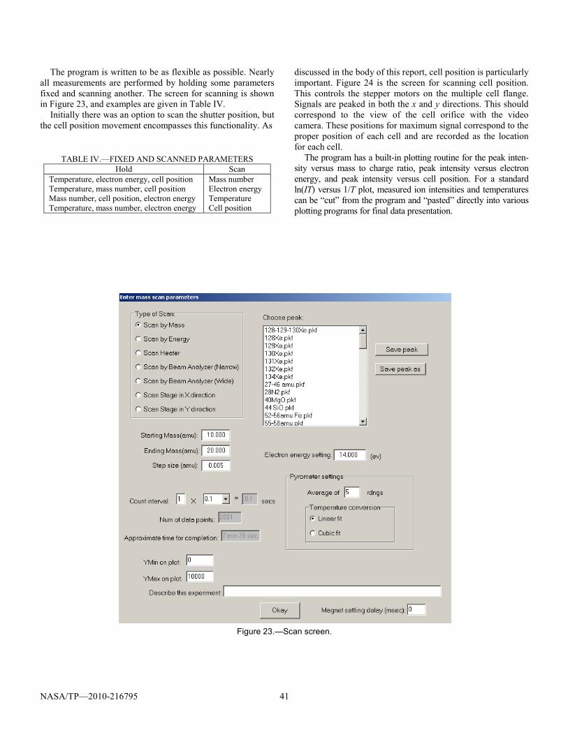
NASA/TP—2010-216795 41

The program is written to be as flexible as possible. Nearly all measurements are performed by holding some parameters fixed and scanning another. The screen for scanning is shown in Figure 23, and examples are given in Table IV.

Initially there was an option to scan the shutter position, but the cell position movement encompasses this functionality. As

TABLE IV.—FIXED AND SCANNED PARAMETERS Hold Scan

Temperature, electron energy, cell position Mass number Temperature, mass number, cell position Electron energy Mass number, cell position, electron energy Temperature Temperature, mass number, electron energy Cell position

discussed in the body of this report, cell position is particularly important. Figure 24 is the screen for scanning cell position. This controls the stepper motors on the multiple cell flange. Signals are peaked in both the x and y directions. This should correspond to the view of the cell orifice with the video camera. These positions for maximum signal correspond to the proper position of each cell and are recorded as the location for each cell.

The program has a built-in plotting routine for the peak inten-sity versus mass to charge ratio, peak intensity versus electron energy, and peak intensity versus cell position. For a standard ln(IT) versus 1/T plot, measured ion intensities and temperatures can be “cut” from the program and “pasted” directly into various plotting programs for final data presentation.

Figure 23.—Scan screen.

NASA/TP—2010-216795 42

Figure 24.—Screen showing x-y table position.

NASA/TP—2010-216795 43

References 1. Misra, A.K.: Thermodynamic Analysis of Compatibility of Several

Reinforcement Materials With Beta Phase NiAl Alloys, Final Report. NASA CR–4171, 1988.

2. Saunders, N.; and Miodownik, A.P.: CALPHAD, Calculation of Phase Diagrams, A Comprehensive Guide. Elsevier Science Ltd., Oxford, U.K., 1998.

3. Kato, Eiichi: Thermodynamic Studies of Metallurgical Systems by Mass Spectrometry. J. Mass Spectrom. Soc. Jpn., vol. 41, no. 6, 1993, pp. 297–316.

4. Hilpert, K.: High Temperature Mass Spectrometry in Materials Research. Rapid Commun. Mass Spectrom., vol. 5, no. 4, 1991, pp. 175–187.

5. Chatillon, Christian, et al.: High-Temperature Mass Spectrometry With the Knudsen-Cell: II. Technical Constraints in the Multiple-Cell Method for Activity Determinations. High Temperatures—High Pressures, vol. 34, no. 2, 2002, pp. 213–233.

6. Knudsen, Martin: Die Gesetze der Molekularströmung und der inneren Reibungsströmung der Gase durch Röhren. Annalen der Physik, vol. 333, no. 1, 1909, pp. 75–130.

7. Chang, Y. Austin; and Oats, Alan: Materials Thermodynamics. John Wiley, Hoboken, NJ, 2010.

8. Lewis, Gilbert Newton; and Randall, Merle: Thermodynamics. Second ed., revised by Kenneth S. Pitzer and Leo Brewer, McGraw-Hill, New York, NY, 1961.

9. Lupis, C.H.P.: Chemical Thermodynamics of Materials. North-Holland, New York, NY, 1983.

10. Kubachewski, O.; and Alcock, C.B.: Metallurgical Thermochemi-stry. Fifth ed., Pergamom Press, Oxford, U.K., 1979.

11. Ionov, N.I.: Ionization of KI, NaI, and CsCl Molecules by Electrons. Doklady Akademii Nauk S.S.S.R., vol. 59, 1948, pp. 467–469.

12. Inghram, M.G.; and Drowart, J.: Mass Spectrometry Applied to High Temperature Chemistry. Proceedings of an International Symposium on High Temperature Technology, McGraw-Hill Book Company, New York, NY, 1960.

13. Drowart, J.; and Goldfinger, P.: Investigation of Inorganic Systems at High Temperature by Mass Spectrometry. Angew. Chem. Int. Ed., vol. 6, no. 7, 1967, pp. 581–648.

14. Grimley, Robert T.: Mass Spectrometry. The Characterization of High-Temperature Vapors, John L. Margrave, ed., John Wiley & Sons, New York, NY, 1967, pp. 195–243.

15. Cater, E. David: Measurement of the Gross Equilibrium Vaporization Rate (Knudsen Methods). Physicochemical Meas-urements in Metals Research, Robert Anthony Rapp, ed., Interscience Publishers, New York, NY, 1970, pp. 21–94.

16. Cater, E. David: The Effusion Method at Age 69: Current State of the Art. Characterization of High Temperature Vapors and Gases, vol. I, U.S. Department of Commerce, National Bureau of Stan-dards, 1979, pp. 3–38.

17. Drowart, Jean, et al.: High-Temperature Mass Spectrometry: Instrumental Techniques, Ionization Cross-Sections, Pressure Measurements, and Thermodynamic Data (IUPAC Technical Report), Pure Appl. Chem., vol. 77, no. 4, 2005, pp. 683–737.

18. Stolyarova, V.L.; and Semenov, G.A.: Mass Spectrometric Study of the Vaporization of Oxide Systems. Wiley, New York, NY, 1994.

19. Jeans, James Hopwood: An Introduction to the Kinetic Theory of Gases. Cambridge University Press, London, U.K., 1962.

20. Loeb, Leonard B.: The Kinetic Theory of Gases. Third ed., Dover Publications, New York, NY, 1961.

21. Rosenblatt, Gerd M.: Evaporation from Solids. Treatise on Solid State Chemistry. Vol. 6A, N.B. Hannay, ed., Plenum Press, New York, NY, 1976, pp. 165–240.

22. Searcy, A.W.: Kinetics of Evaporation and Condensation Reactions. Chemical and Mechanical Behavior of Inorganic Mate-rials, Alan W. Searcy, David V. Ragone, and Umberto Colombo, eds., Wiley-Interscience, New York, NY, 1970, pp. 107–133.

23. Clausing, P.: Over de Stationnaire Strooming van Zeer Verdunde Gassen. Ph.D. Thesis, Eindhoven, 1929.

24. Clausing, P.: Uber die Strahlformung bei der Molekularstromung. Z. Angew. Phys., 1930, pp. 471–476.

25. DeMarcus, W.C.: The Problem of Knudsen Flow. Oak Ridge Gaseous Diffusion Plant Report K–1302, pts. I–VI, 1956/1957.

26. Freeman, Robert D.; and Edwards, Jimmie G.: Transmission Probabilities and Recoil Force Correction Factors for Conical Orifices. The Characterization of High-Temperature Vapors, John L. Margrave, ed., John Wiley & Sons, New York, NY, 1967, pp. 508–527.

27. Grimley, Robert T.; Wagner, L.C.; and Castle, Peter M.: Angular Distributions of Molecular Species Effusing From Near-Ideal Ori-fices. J. Phys. Chem., vol. 79, no. 4, 1975, pp. 302–308.

28. Davis, D.H.: Monte Carlo Calculation of Molecular Flow Rates through a Cylindrical Elbow and Pipes of Other Shapes. J. Appl. Phys., vol. 31, no. 7, 1960, pp. 1169–1176.

29. Ward, J.W.; Mulford, R.N.R.; and Bivins, R.L.: Study of Some of the Parameters Affecting Knudsen Effusion. II. A Monte Carlo Computer Analysis of Parameters Deduced from Experiment. J. Chem. Phys., vol. 47, 1967, pp. 1718–1723.

30. Jacobson, Nathan S.: The Diffusion of Gases Through Capillaries. Ph.D. Thesis. University of California, Berkeley, 1981.

31. Jacobson, N.S.: Monte Carlo Simulation of Knudsen Effusion. Unpublished work, 2004.

32. Whitman, Charles I.: On the Measurement of Vapor Pressures by Effusion. J. Chem. Phys., vol. 20, no. 1, 1952, pp. 161–164.

33. Motzfeldt, Ketil: The Thermal Decomposition of Sodium Carbonate by the Effusion Method. J. Phys. Chem., vol. 59, no. 2, 1955, pp. 139–147.

34. Hollahan, John R.: Molecular Effusion: Its Newer Features and Applications. J. Chem. Educ., vol. 39, no. 1, 1962, pp. 23–26.

35. Rosenblatt, Gerd M.: Effect of Restrictions to Molecular Flow Upon Measurements of Vaporization Rate and Vapor Pressure. J. Phys. Chem., vol. 71, no. 5, 1967, pp. 1327–1333.

36. Rocabois, Philippe; Chatillon, Christian; and Bernard, Claude: Thermodynamics of the Si–C System I. Mass Spectrometric Studies of the Condensed Phases at High Temperature. High Temperatures—High Pressures, vols. 27/28, 1995/1996, pp. 3–23.

37. Rocabois, P.; Chatillon, C.; and Bernard, C.: Thermodynamics of the Si-O-N System: I. High-Temperature Study of the Vaporization Behavior of Silicon Nitride by Mass Spectrometry. J. Am. Ceram. Soc., vol. 79, no. 5, 1996, pp. 1351–1360.

38. Copland, E.: Comparing the Thermodynamic Behavior of Al(l) + ZrO2(4% Y2O3) and Al(l) + Al2O3(s). Int. J. Mater. Res., vol. 97, 2006, pp. 1108–1114.

39. Copland, Evan: Vapor Pressures in the Al(l) + Al2O3(s) System: Reconsidering Al2O3(s) Condensation. J. Chem. Thermodyn., vol. 38, no. 4, 2006, pp. 443–449.

NASA/TP—2010-216795 44

40. Belov, A.N.; and Semenov, G.A.: Thermodynamics of Binary Solid Solutions of Zirconium, Hafnium, and Yttrium Oxides from High-Temperature Mass Spectrometry Data. Russ. J. Phys. Chem., vol. 59, no. 3, 1985, pp. 342–344.

41. Zmbov, K.F.; Ames, L.L.; and Margrave, J.L.: A Mass Spectro-metric Study of the Vapor Species Over Silicon and Silicon Oxides. High Temp. Sci., vol. 5, 1973, pp. 235–240.

42. Kohl, F.J.; and Stearns, C.A.: Vaporization Dissociation Energies of the Molecular Carbides of Titanium, Zirconium, Hafnium, and Thorium. High Temp. Sci., vol. 6, no. 4, 1974, pp. 284–302.

43. Eckert, M., et al.: Thermodynamic Activities in the Alloys of the Ti-Al System. Ber. Bunsen Ges., vol. 100, no. 4, 1996, pp. 418–424.

44. Storms, E.: Some Effects of a Temperature Gradient on Knudsen Effusion. High Temp. Sci., vol. 1, 1969, pp. 456–465.

45. Chatillon, C., et al.: High-Temperature Thermodynamical Studies by Mass Spectrometry: Use of Heat Pipe Devices To Main-tain Isothermal Conditions in Effusion Cells. J. Appl. Phys., vol. 47, no. 4, 1976, pp. 1690–1693.

46. Preston-Thomas, H.: International Temperature Scale of 1990 (ITS–90). Metrologia, vol. 27, 1990, pp. 3–10.

47. McGlashan, M.L.: The International Temperature Scale of 1990 (ITS–90). J. Chem. Thermodyn., vol. 22, no. 7, 1990, pp. 653–663.

48. Bedford, R.E., et al.: Recommended Values of Temperature on the International Temperature Scale of 1990 for a Selected Set of Secondary Reference Points. Metrologia, vol. 33, no. 2, 1996, pp. 133–154.

49. Walker, Raymond F.: Temperature Measurement in High Tem-perature Chemistry: 1 000–3 000° C. Rev. Hautes Temper. et Refract., vol. 3, 1966, pp. 301–308.

50. Wensel, H.T.: Temperature. Temperature, Its Measurement and Control In Science and Industry. Reinhold Publishing Corp., New York, NY, 1941, pp. 3–23.

51. Copland, Evan H.: Long Term Measurement of the Vapor Pressure of Gold in the Au-C System; Final Report. NASA/CR—2009-215498, 2009.

52. Manual on the Use of Thermocouples in Temperature Meas-urement. ASTM Special Technical Publication 470, American Society for Testing Materials, Philadelphia, PA, 1994.

53. Morland, Peter; Chatillon, Christian; and Rocabois, Philippe: High-Temperature Mass Spectrometry Using the Knudsen Effusion Cell, I—Optimization of Sampling Constraints on the Molecular Beam. High Temp. Mater. Sci., vol. 37, no. 3, 1997, pp. 167–187.

54. Walsh, John W.T.: Radiation From a Perfectly Diffusing Circular Disc (Part I). Proc. Phys. Soc. London, vol. 32, 1919, p. 59.

55. Walsh, John W.T.: Photometry. Constable & Company, London, UK, 1958, pp. 136–144.

56. Roboz, John: Introduction to Mass Spectrometry; Instrumentation and Techniques. Interscience Publishers, New York, NY, 1968.

57. Dahl, David A.: Simion 3D, Version 7.0, User’s Manual. INEEL–95/0403 (formerly EGG-C7–7233), Rev. 5, 2000.

58. Morrison, J.D.: Application of the Mass Spectrometer to the Study of the Upper Energy States of Molecules. J. Appl. Phys., vol. 28, 1957, pp. 1409–1413.

59. Kieffer, Lee Joseph; and Dunn, G.H.: Electron Impact Ionization Cross-Section Data for Atoms, Atomic Ions, and Diatomic Molecules: I. Experimental Data. Joint Institute for Laboratory Astrophysics Report 51, University of Colorado, Boulder, 1965.

60. Morrison, J.D.: Studies of Ionization Efficiency. I. The Determina-tion of Molecular Appearance Potentials Using the Mass Spectrom-eter. J. Chem. Phys., vol. 19, no. 10, 1951, pp. 1305–1308.

61. Simpson, J. Arol; and Kuyatt, C.E.: Anomalous Energy Spreads in Electron Beams. J. Appl. Phys., vol. 37, no. 10, 1966, pp. 3805–3809.

62. Fischer, M.: Kinetic Theory of the Energy Spread in Electron Beams. J. Appl. Phys., vol. 41, no. 9, 1970, pp. 3615–3620.

63. Otvos, J.W.; and Stevenson, D.P.: Cross-Sections of Molecules for Ionization by Electrons. J. Am. Chem. Soc., vol. 78, no. 3, 1956, pp. 546–551.

64. Mann, Joseph B.: Ionization Cross Sections of the Elements Calcu-lated from Mean-Square Radii of Atomic Orbitals. J. Chem. Phys., vol. 46, no. 5, 1967, pp. 1646–1651.

65. Gryzinski, Michal: Classical Theory of Atomic Collisions. I. Theory of Inelastic Collisions. Physical Review, vol. 138, no. 2A, 1965, pp. A336–A358.

66. Deutsch, H., et al.: A Detailed Comparison of Calculated and Measured Electron-Impact Ionization Cross Sections of Atoms Using the Deutsch-Märk Formalism. Int. J. Mass Spectrom., vol. 243, 2005, pp. 215–221.

67. Schroeer, Juergen M.; Gunduz, Dincer H.; and Livingston, Spencer: Electron Impact Ionization Cross Sections of Cu and Au Between 40 and 250 eV, and the Velocity of Evaporated Atoms. J. Chem. Phys., vol. 58, no. 11, 1973, pp. 5135–5140.

68. Brook, E.; Harrison, M.F.A.; and Smith, A.C.H.: Measurements of the Electron Impact Ionisation Cross Sections of He, C, O and N Atoms. J. Phys. B: Atom. Molec. Phys., vol. 11, no. 17, 1978, pp. 3115–3132.

69. Hayes, Todd R., et al.: Absolute Cross Sections for Electron-Impact Ionization and Dissociative Ionization of the SiF Free Radical. J. Chem. Phys., vol. 88, no. 2, 1988, pp. 823–829.

70. Wetzel, Robert C., et al.: Absolute Cross Sections for Electron-Impact Ionization of the Rear-Gas Atoms by the Fast-Neutral-Beam Method. Phys. Rev. A: At. Mol. Opt. Phys., vol. 35, no. 2, 1987, pp. 559–577.

71. Freund, Robert S., et al.: Cross-Section Measurements for Electron-Impact Ionization of Atoms. Phys. Rev. A: At. Mol. Opt. Phys., vol. 41, no. 7, 1990, pp. 3575–3595.

72. Cooper, John L., Jr.; Pressley, George A., Jr.; and Stafford, Fred E.: Electron-Impact Ionization Cross Sections for Atoms. J. Chem. Phys., vol. 44, no. 10, 1966, pp. 3946–3949.

73. Pottie, R.F.: Cross Sections for Ionization by Electrons. I. Absolute Ionization Cross Sections of Zn, Cd, and Te2. II. Comparison of Theoretical with Experimental Values for Atoms and Molecules. J. Chem. Phys., vol. 44, no. 3, 1966, pp. 916–922.

74. Alcock, Charles B.: Relative Ionization Efficiencies From Alloy Thermodynamic Data. High Temperatures—High Pressures, vol. 20, 1988, pp. 165–168.

75. Gingerich, Karl A.; and Blue, Gary D.: Experimental Relative Electron Impact Cross Sections for Group-III Metal Atoms and Comparison with Theories. J. Chem. Phys., vol. 53, 1970, pp. 4713–4714.

76. Blackburn, P.E.; and Danielson, P.M.: Electron Impact Relative Ionization Cross Sections and Fragmentation of U, UO, UO2, and UO3. J. Chem. Phys., vol. 56, no. 12, 1972, pp. 6156–6164.

77. Kohl, Fred J.; Uy, O. Manuel; and Carlson, K. Douglas: Cross Sec-tions for Electron-Impact Fragmentation and Dissociation Energies of the Dimer and Tetramer of Bismuth. J. Chem. Phys., vol. 47, no. 8, 1967, pp. 2667–2676.

78. Leo, William R.: Techniques for Nuclear and Particle Physics Experiments: A How-To Approach. Second ed., Springer-Verlag, Berlin, 1994.

NASA/TP—2010-216795 45

79. Dietz, Leonard A.: Basic Properties of Electron Multiplier Ion Detection and Pulse Counting Methods in Mass Spectrometry. Rev. Sci. Instrum., vol. 36, 1965, pp. 1763–1770.

80. Chatillon, C.; Allibert, M.; and Pattoret, A.: Thermodynamic and Physico-Chemical Behavior of the Interactions Between Knudsen-Effusion-Cells and the Systems Under Investigation, Analysis by High Temperature Mass Spectrometry. National Bureau of Stan-dards Special Publication 561/1, 1979, p. 181.

81. Dunn, Gordon H.; and Van Zyl, Bert: Electron Impact Dissociation of H2

+. Physical Review, vol. 154, no. 1, 1967, pp. 40–51. 82. Muller, A., et al.: An Improved Crossed-Beams Technique for

the Measurement of Absolute Cross Sections for Electron Impact Ionisation of Ions and Its Application to Ar+ Ions. J. Phys. B: At. Mol. Phys., vol. 18, 1985, pp. 2993–3009.

83. Cubicciotti, Daniel: A New Σ-Plot Treatment of Equilibrium Data and Its Application to the Vaporization of Bismuth Chloride. J. Phys. Chem., vol. 70, no. 7, 1966, pp. 2410–2413.

84. Horton, William S.: Statistical Aspects of Second and Third Law Heats. J. Res. Nat. Bur. Stand., vol. 70A, no. 6, 1966, pp. 533–539.

85. Albers, M., et al.: Chemical Activities in the Solid Solution of Hf in Ni3Al. Ber. Bunsen Ges. Phys. Chem., vol. 96, no. 11, 1992, pp. 1663–1668.

86. Lee, Marvin C.Y.; and Adams, Arnold: A Combination Compact Knudsen Cell-Mass Spectrometer Apparatus for Alloy Studies. High Temp. Sci., vol. 25, no. 2, 1988, pp. 103–116.

87. Lyubimov, A.P.; Zobens, V. Ya; and Rakhovskii, V.I.: A Mass Spectrometric Determination of the Thermodynamic Characteris-tics of Binary Metallic Systems. Zhur. Fiz. Khim., vol. 32, 1958, pp. 1804–1808.

88. Belton, Geoffrey R.; and Fruehan, Richard J.: Determination of Activities by Mass Spectrometry. I. The Liquid Metallic Systems Iron-Nickel and Iron-Cobalt. J. Phys. Chem., vol. 71, no. 5, 1967, pp. 1403–1409.

89. Neckel, Von A.; and Wagner, Sigurd: Massenspektrometrische Bestimmung Thermodynamischer Aktivitäten, I. Das System Gold-Kupfer. Ber. Bunsen Ges. Phys. Chem., vol. 73, no. 2, 1969, pp. 210–217.

90. Jacobson, Nathan S.; and Mehrotra, Gopal M.: Thermodynamics of Iron-Aluminum Alloys at 1573 K. Metall. Trans. B, vol. 24B, 1993, pp. 481–486.

91. Belton, G.R.; and Fruehan, R.J.: Determination of Activities by Mass-Spectrometry, Some Additional Methods. Met. Trans., vol. 2, no. 1, 1971, pp. 291–296.

92. Neckel, A.: Mass-Spectrometric Determination of Thermodynamic Mixing Effects of Alloys. Thermochemistry of Alloys, H. Brodowsky and H.-J. Schaller, eds., Kluwer Academic Publishers, Dordrecht, 1989, pp. 221–246.

93. Gokcen, N.A.; Chang, E.T.; and Marx, P.C.: Novel Uses of Knudsen Cells at High Temperatures. High Temperature Tech-nology, Butterworth & Co., London, 1969, pp. 611–627.

94. Nunoue, Shin-Ya; and Kato, Eiichi: Mass Spectrometric Study of the Partial Phase Diagram of the Fe-Ge System Above 1050 °C. Metall. Trans. A, vol. 20 A, 1989, pp. 975–976.

95. Copland, Evan: Solidification Behavior of γ′ -Ni3Al-Containing Alloys in the Ni-Al-O System. Acta Mater., vol. 55, 2007, pp. 4853–4865.

96. Berkowitz, J.; and Chupka, W.: Composition of Vapors in Equili-brium With Salts at High Temperatures. Ann. N.Y. Acad. Sci., vol. 79, 1960, pp. 1073–1078.

97. Johnston, G.R.; and Burley, N.A.: Quad-Cell Mass Spectrometry: Vaporization Studies up to 2300 K Using a Rotatable, Multiple Knudsen Cell (‘QUAD-CELL’). Proceedings of the Seventh Sym-posium on Thermophysical Properties. Ared Cezairliyan, ed., American Society of Mechanical Engineers, New York, NY, 1977, pp. 222–230.

98. Raychaudhuri, P.K.; and Stafford, F.E.: Alloy Thermodynamics by Mass Spectrometry: A Critical Review. Mater. Sci. Eng., vol. 20, no. 1, 1975, pp. 1–18.

99. Stickney, Michael J.; Chandrasekharaiah, Mallasetty S.; and Gingerich, Karl A.: Twin-Chamber Knudsen-Effusion-Cell Mass Spectrometer for Thermodynamic Studies of Alloys. High Temperatures—High Pressures, vol. 20, 1988, pp. 627–635.

100. Copland, Evan: Partial Thermodynamic Properties of γ ′-(Ni,Pt)3Al in the Ni-Al-Pt System. J. Phase Equilib. Diffus., vol. 28, no. 1, 2007, pp. 38–48.

101. Copland, Evan: Dissolved Oxygen and the Partial Thermodynamic Properties of γ′-Ni3Al + β-NiAl Alloys. Scripta Mater., vol. 57, no. 1, 2007, pp. 21–24.

102. Copland, Evan: Thermodynamic Effect of Platinum Addition to β−NiAl: An Initial Investigation. NASA/CR—2005-213330, 2005.

103. Paule, Robert C.; and Mandel, John: Analysis of Interlaboratory Measurements on the Vapor Pressure of Gold. Pure Appl. Chem., vol. 31, 1972, pp. 371–394.

104. Zaitsev, A.I.; Zemchenko, M.A.; and Mogutnov, B.M.: Thermody-namic Properties of the Alloys (1–x)Cr + xMn. J. Chem. Thermodynamics, vol. 22, no. 1, 1990, pp. 41–53.

105. Pahlman, J.E.; and Smith, J.F.: Thermodynamics of Formation of Compounds in the Ce-Mg, Nd-Mg, Gd-Mg, Dy-Mg, Er-Mg, and Lu-Mg Binary Systems in the Temperature Range 650° to 930°K. Met. Trans., vol. 3, no. 9, 1972, pp. 2423–2432.

106. Ciccioli, A., personal communication, 2010. 107. Detry, D., et al.: Zur Thermodynamik von Schwefeldampf,

Massenspektrometrishe Untersuchungen mit der Knudsen-Zelle. Z. Phys. Chem., vol. 55, 1967, pp. 314–319.

108. Keller, H., et al.: Zur Thermodynamik von Selendampf, Massenspektrometrische Untersuchungen mit der elektro-chemischen Knudsen-Zelle. Z. Phys. Chem., vol. 75, 1971, pp. 273–286.

109. Manura, D.; and Dahl, D.: SIMION Version 8.0 User Manual. Scientific Instrument Services, Ringoes, NJ, 2008.

110. Dunn, Gordon H.; and Van Zyl, Bert: Electron Impact Dissociation of H2

+. Phys. Rev., vol. 154, no. 1, 1967, pp. 40–51. 111. Wyatt, J.R.; Pressley, G.A., Jr.; and Stafford, F.E.: On-line Com-

puter Control and Data Acquisition for a High Tempera-ture/Molecular Beam Mass Spectrometer. High Temperature Science, vol. 3, no. 2, 1971, pp. 130–137.

112. Liu, Norman W.K.; and Muenow, David W.: A Control and Data Acquisition for a High-Temperature Knudsen-Cell Quadrupole Mass Spectrometer. High Temp. Sci., vol. 10, 1978, pp. 145–153.

113. Instruction Manual for General Purpose Physical Chemistry/Mass Spectroscopy Software. Version 3.5, Measurement and Analysis Systems, Inc., Bellefonte, PA, and Lowell, MA, 1989.

114. User’s Guide to Program HTMS Analysis: A Computer Program to Process and Display Nuclide High Temperature Mass Spectra. Version 1.0, Corning Incorporated, Corning, NY, 1994.

115. Borland Delphi 7 Professional. Embarcadero Technologies, Inc., San Francisco, CA, 2010.

REPORT DOCUMENTATION PAGE Form Approved

OMB No. 0704-0188 The public reporting burden for this collection of information is estimated to average 1 hour per response, including the time for reviewing instructions, searching existing data sources, gathering and maintaining the data needed, and completing and reviewing the collection of information. Send comments regarding this burden estimate or any other aspect of this collection of information, including suggestions for reducing this burden, to Department of Defense, Washington Headquarters Services, Directorate for Information Operations and Reports (0704-0188), 1215 Jefferson Davis Highway, Suite 1204, Arlington, VA 22202-4302. Respondents should be aware that notwithstanding any other provision of law, no person shall be subject to any penalty for failing to comply with a collection of information if it does not display a currently valid OMB control number. PLEASE DO NOT RETURN YOUR FORM TO THE ABOVE ADDRESS.

1. REPORT DATE (DD-MM-YYYY) 01-11-2010

2. REPORT TYPE Technical Paper

3. DATES COVERED (From - To)

4. TITLE AND SUBTITLE Measuring Thermodynamic Properties of Metals and Alloys With Knudsen Effusion Mass Spectrometry

5a. CONTRACT NUMBER

5b. GRANT NUMBER

5c. PROGRAM ELEMENT NUMBER

6. AUTHOR(S) Copland, Evan, H.; Jacobson, Nathan, S.

5d. PROJECT NUMBER

5e. TASK NUMBER

5f. WORK UNIT NUMBER WBS 599489.02.07.03.02.11.02

7. PERFORMING ORGANIZATION NAME(S) AND ADDRESS(ES) National Aeronautics and Space Administration John H. Glenn Research Center at Lewis Field Cleveland, Ohio 44135-3191

8. PERFORMING ORGANIZATION REPORT NUMBER E-17245

9. SPONSORING/MONITORING AGENCY NAME(S) AND ADDRESS(ES) National Aeronautics and Space Administration Washington, DC 20546-0001

10. SPONSORING/MONITOR'S ACRONYM(S) NASA

11. SPONSORING/MONITORING REPORT NUMBER NASA/TP-2010-216795

12. DISTRIBUTION/AVAILABILITY STATEMENT Unclassified-Unlimited Subject Category: 26 Available electronically at http://gltrs.grc.nasa.gov This publication is available from the NASA Center for AeroSpace Information, 443-757-5802

13. SUPPLEMENTARY NOTES The main part of this document will also appear in “Applied Mass Spectroscopy Handbook,” ed. M. Lee, Wiley, 2010, in press, as the chapter “Measuring Thermodynamic Properties of Metals and Alloys.”

14. ABSTRACT This report reviews Knudsen effusion mass spectrometry (KEMS) as it relates to thermodynamic measurements of metals and alloys. First, general aspects are reviewed, with emphasis on the Knudsen-cell vapor source and molecular beam formation, and mass spectrometry issues germane to this type of instrument are discussed briefly. The relationship between the vapor pressure inside the effusion cell and the measured ion intensity is the key to KEMS and is derived in detail. Then common methods used to determine thermodynamic quantities with KEMS are discussed. Enthalpies of vaporization ΔvapH

oT--the fundamental measurement--are determined from the variation of relative

partial pressure with temperature using the second-law method or by calculating a free energy of formation and subtracting the entropy contribution using the third-law method. For single-cell KEMS instruments, ΔvapH

oT measurements can be used to determine the partial

Gibbs free energy if the sensitivity factor remains constant over multiple experiments. The ion-current ratio method and dimer-monomer method are also viable in some systems. For a multiple-cell KEMS instrument, ΔvapH

oT and activities are obtained by direct comparison

with a suitable component reference state or a secondary standard. Internal checks for correct instrument operation and general procedural guidelines also are discussed. Finally, general comments are made about future directions in measuring alloy thermodynamics with KEMS.15. SUBJECT TERMS Metals; Alloys; Thermodynamics; Mass spectroscopy

16. SECURITY CLASSIFICATION OF: 17. LIMITATION OF ABSTRACT UU

18. NUMBER OF PAGES

50

19a. NAME OF RESPONSIBLE PERSON STI Help Desk (email:help@sti.nasa.gov)

a. REPORT U

b. ABSTRACT U

c. THIS PAGE U

19b. TELEPHONE NUMBER (include area code) 443-757-5802

Standard Form 298 (Rev. 8-98)Prescribed by ANSI Std. Z39-18