Embed Size (px)
Citation preview
Measuring Texture and Color inImages
Avinash Kak
Purdue University
October 11, 2018
1:15pm
An RVL Tutorial Presentation
Originally presented in Fall 2016. Code examples updated in January 2018
Minor fixes in October 2018
c©2018 Avinash Kak, Purdue University
CONTENTS
Section Title Page
1 Does the World Really Need Yet Another Tutorial? 3
2 Characterizing Image Textures 4
3 Characterizing a Texture with a Gray-Level 8Co-Occurrence Matrix (GLCM)
3.1 Summary of GLCM Properties 173.2 Deriving Texture Measures from GLCM 193.3 Python Code for Experimenting with GLCM 24
4 Characterizing Image Textures with Local 28Binary Pattern (LBP) Histograms
4.1 Characterizing a Local Inter-Pixel Gray-Level 30Variation with a Contrast-Change-InvariantBinary Pattern
4.2 Generating Rotation-Invariant Representations 35from Local Binary Patterns
4.3 Encoding the minIntVal Forms of LBP 384.4 Python Code for Experimenting with LBP 47
5 Characterizing Image Textures with a Gabor 51Filter Family
5.1 A Brief Review of 2D Fourier Transform 555.2 The Gabor Filter Operator 575.3 Python Code for Experimenting with Gabor 69
Filter Banks
6 Dealing with Color in Images 74
6.1 What Makes Learning About Color So Frustrating 776.2 Our Trichromatic Vision and the RGB Model 826.3 Color Spaces 886.4 The Great Difficulty of Measuring the True 118
Color of an Object Surface
2

Texture and Color An RVL Tutorial by Avi Kak
1: Does the World Really Need Yet AnotherTutorial?
• The main reason for this tutorial is for it to serve as a handout for
Lecture 15 of my class on Computer Vision at Purdue University.
Here is a link to the course website so that you can see for yourself
where this lecture belongs in an overall organization of the course:
https://engineering.purdue.edu/kak/computervision/ECE661Folder
• All of the code examples you see in this tutorial can be down-
loaded as a gzipped tar archive from
https://engineering.purdue.edu/kak/distTextureAndColor/CodeForTextureAndColorTutorial.tar.gz
• PLEASE HELP! Since this is an early draft of this tutorial,
I am sure it contains typos, inadvertently skipped words (the
fingers-on-a-keyboard-not-keeping-up-with-the-brain phenomenon),
poor phrasing (the dumb-ass-attack phenomenon), spelling errors
(the we-are-losing-our-ability-to-spell-correctly-because-of-auto-spell-
checkers phenomenon), and so on. Please let me know (email:
[email protected]) if you see any such defects in this document. If
you do send email, please be sure to place the string “Texture
and Color” in the Subject line to get past my pretty strong spam
filter.
3
Texture and Color An RVL Tutorial by Avi Kak
2: Characterizing Image Textures
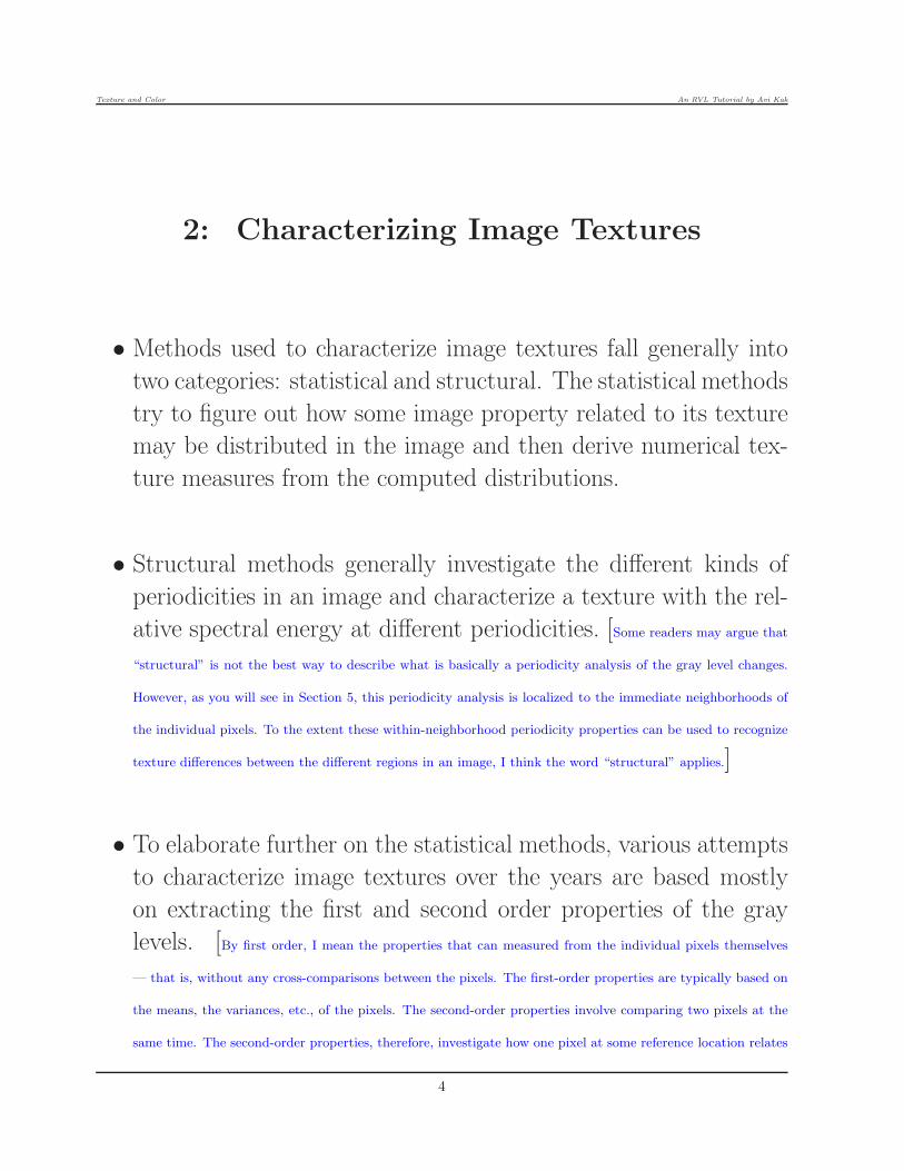
• Methods used to characterize image textures fall generally into
two categories: statistical and structural. The statistical methods
try to figure out how some image property related to its texture
may be distributed in the image and then derive numerical tex-
ture measures from the computed distributions.
• Structural methods generally investigate the different kinds of
periodicities in an image and characterize a texture with the rel-
ative spectral energy at different periodicities. [Some readers may argue that
“structural” is not the best way to describe what is basically a periodicity analysis of the gray level changes.
However, as you will see in Section 5, this periodicity analysis is localized to the immediate neighborhoods of
the individual pixels. To the extent these within-neighborhood periodicity properties can be used to recognize
texture differences between the different regions in an image, I think the word “structural” applies.]
• To elaborate further on the statistical methods, various attempts
to characterize image textures over the years are based mostly
on extracting the first and second order properties of the gray
levels. [By first order, I mean the properties that can measured from the individual pixels themselves
— that is, without any cross-comparisons between the pixels. The first-order properties are typically based on
the means, the variances, etc., of the pixels. The second-order properties involve comparing two pixels at the
same time. The second-order properties, therefore, investigate how one pixel at some reference location relates
4

Texture and Color An RVL Tutorial by Avi Kak
statistically to another pixel at a location displaced from the reference location. Some researchers have also
looked at characterizing textures with third and higher order properties. These would involve investigating the
gray level distributions at three or more pixels whose coordinates must occupy specific positions vis-a-vis one
another. Third and higher order texture characterizations have been found to be too complex for a practical
characterization of textures.]
• In what follows, GLCM and LBP are examples of texture char-
acterizations based on their second-order statistical properties.
On the other hand, the technique based on Gabor filters is an
example of the structural approach.
• Any numerical characterization of image textures must possess
some essential properties in order to be useful in practical appli-
cations:
– To the maximum extent possible, it must be invariant to
changes in image contrast that may be produced by chang-
ing or uneven illumination of a scene — assuming that the
texture remains more or less the same as perceived by a hu-
man. At the least, the numerical characterization must be
invariant to monotonic transformation of the gray scale.
– To the maximum extent possible, it must be invariant to in-
plane rotations of the image.
– It must lend itself to fast computation
5

Texture and Color An RVL Tutorial by Avi Kak
• The first invariance is important because one can certainly expect
that the illumination conditions under which the training data
was collected for a machine learning algorithm may not be the
same as the conditions under which the test data was recorded.
• The same goes for the second invariance: It’s highly likely that
the orientation of the texture you used for training a machine
learning algorithm would not be identical to the orientations of
the same texture in the test images.
• Some researchers have suggested histogram-equalization as an
image normalization tool before subjecting the images to the ex-
traction of texture based properties. Although histogram equal-
ization is a powerful tool for improving the quality of low-contrast
images, its usefulness as a normalizer of images prior to texture
characterization is open to question. In general, histogram equal-
ization results in a nonlinear transformation of the gray scale
and, again in general, such nonlinear transformations can alter
the texture in the original images. Additionally, while histogram
equalization may balance out the contrast variations in a single
image, it does not normalize out image-to-image variations.
• So it is best if the method used for characterizing a texture is
mostly independent of the macro-level variations in the contrast
in each image. That is, we want methods that extract texture
related information from just the changes in the gray levels at the
6

Texture and Color An RVL Tutorial by Avi Kak
level of pixels and their immediate neighborhoods.
7

Texture and Color An RVL Tutorial by Avi Kak
3: CHARACTERIZING A TEXTUREWITH A GRAY-LEVEL
CO-OCCURRENCE MATRIX (GLCM)
• The basic idea of GLCM is to estimate the joint probability dis-
tribution P [x1, x2] for the gray levels in an image, where x1 is
the gray level at any randomly selected pixel in the image and x2
the gray level at another pixel that is at a specific vector distance
d from the first pixel. [You are surely familiar with the histogram P [x] of gray
levels in an image: P [x] is the probability that the gray level at a randomly chosen
pixel in the image will equal x. That is, if you count the number of pixels at gray level
x and divide that count by the total number of pixels, you get P [x]. Now extend that
concept to examining the gray levels at two different pixels that are separated by a
displacement vector d. If you count the number of pairs of pixels that are d apart, with
one pixel at gray level x1 and the other at gray level x2, and you normalize this count
by the total number of pairs of pixels that are d apart, you’ll get P [x1, x2].] After
you have estimated P [x1, x2], the texture can be characterized
by the shape of this joint distribution.
• Therefore, thinking about the gray levels at two different pixels
that are separated by a fixed displacement vector d is a good
place to start for understanding the GLCM approach to texture
characterization.
8

Texture and Color An RVL Tutorial by Avi Kak
• Let’s say we raster scan an image left to right and top to bottom
and we examine the gray level at each pixel that we encounter
and at another pixel that at a displacement d with respect to the
first pixel. [Assume that as we are scanning an image, we are currently at the pixel
coordinates (i, j). As far as the displacement d is concerned, it could be as simple as
pointing to the next pixel, the one at (i, j + 1), or, as simple as pointing to the pixel
that is one column to the right and one row below. For the first case, d = (0, 1) and for
the second case d = (1, 1).]
• As an image is being scanned, the (m,n)-th element of the GLCM
matrix records the number of times we have seen the following
event: the gray level at the current pixel is m while the gray level
at the d-displaced pixel is n.
• To illustrate with a toy example, consider the following 4 × 4
image with pixels whose gray levels come from the set {0, 1, 2}:
2 0 1 1
0 1 2 0
1 1 1 2
0 0 1 1
• And let us assume a displacement vector of
d = (1, 1) (1)
9

Texture and Color An RVL Tutorial by Avi Kak
As we scan the image row by row by visiting each pixel from top
left to bottom right, if m is the gray level at the current pixel
and n the gray level at the pixel one position to the right and one
row below, we increment glcm[m][n] by 1. Scanning the 4 × 4
array shown above, we get the following 3× 3 GLCM matrix:
-----------> displaced pixel
| gray levels
|
| 0 1 1 NOTE: The glcm matrix
| 2 3 0 is of size 3x3
| 0 1 1 because we have
| ONLY 3 gray levels
V which are {0,1,2)
reference pixel
gray levels
• Looking at the first row, what this matrix tells us is that if the ref-
erence pixel has gray level 0, it is never the case that the displaced
pixel also has gray level 0. And that there is only one occurrence
of the reference pixel having gray level 0 while the displaced pixel
has gray level 1. And that there is only one occurrence of the
reference pixel being of gray level 0, while the displaced pixel has
gray level 2.
• Looking at the second row of the GLCM matrix shown above,
there are two occurrences of the reference pixel being 1 while the
displaced pixel has gray level 0. And that are three occurrences
when both the reference and the displaced pixels have gray level
1. And so on.
10

Texture and Color An RVL Tutorial by Avi Kak
• As you would expect, what you get is an asymmetric matrix as
shown above. The matrix is asymmetric because, in general, the
number of times the gray level at the reference pixel is m while
the gray level at the displaced pixel is n will not be the same for
the opposite order of the gray levels at the two pixels.
• Nonetheless, as you will see later, in general one is interested pri-
marily in the fact that two gray levels, m and n, are associated
together because they occur at the two ends of a displacement
vector, and one does not want to be concerned with the order
of appearance of these two gray levels. When that is the case,
it makes sense to create a symmetric GLCM matrix. This can
easily be done by the simple expedient of incrementing the ele-
ment glcm(n,m) when we increment glcm(m,n). For the above
example, this yields the result:
0 3 1
3 6 1
1 1 2
• Here are some interesting observations about GLCM matrices: If
you sum the diagonal elements of a normalized GLCM matrix,
you get the probability that two pixels in the image that are sepa-
rate by the displacement vector d will have identical gray levels —
assuming that the GLCM matrix was constructed for a given dis-
placement d. Along the same lines, if you sum any non-diagonal
entries in the normalized GLCMmatrix that are on a line parallel
11

Texture and Color An RVL Tutorial by Avi Kak
to the diagonal, you get the probability of finding the gray level
difference at any two pixels separated by d corresponding to the
line on which the GLCM elements lie.
• For the example shown above, with a probability of 8/18, two
pixels separated by the displacement d = (1, 1) will have identi-
cal gray levels. Similarly, with a probability of 4/18, two pixels
separated by d = (1, 1) will have their gray level difference equal
to 1.
• The Python script in Section 3.3 allows you to experiment with
different toy textures in images of arbitrary size and with an ar-
bitrary number of gray levels. For example, if you set the texture
type to vertical, the image size to 8 (for an 8 × 8 array), the
number of gray levels to 6, and the displacement vector to (1, 1),
the script yields the output shown below. The first array is the
image array created with the vertical texture that you specified,
and the next array shows the GLCM matrix.
Texture type chosen: vertical
The image:
[5, 0, 5, 0, 5, 0, 5, 0]
[5, 0, 5, 0, 5, 0, 5, 0]
[5, 0, 5, 0, 5, 0, 5, 0]
[5, 0, 5, 0, 5, 0, 5, 0]
[5, 0, 5, 0, 5, 0, 5, 0]
[5, 0, 5, 0, 5, 0, 5, 0]
[5, 0, 5, 0, 5, 0, 5, 0]
[5, 0, 5, 0, 5, 0, 5, 0]
GLCM:
12

Texture and Color An RVL Tutorial by Avi Kak
[0, 0, 0, 0, 0, 49]
[0, 0, 0, 0, 0, 0]
[0, 0, 0, 0, 0, 0]
[0, 0, 0, 0, 0, 0]
[0, 0, 0, 0, 0, 0]
[49, 0, 0, 0, 0, 0]
Texture attributes:
entropy: 1.0
contrast: 25.0
homogeneity: 0.166
• On the other hand, if in the script of Section 3.3, you set the
texture type to horizontal, you get the output shown below:
Texture type chosen: horizontal
The image:
[5, 5, 5, 5, 5, 5, 5, 5]
[0, 0, 0, 0, 0, 0, 0, 0]
[5, 5, 5, 5, 5, 5, 5, 5]
[0, 0, 0, 0, 0, 0, 0, 0]
[5, 5, 5, 5, 5, 5, 5, 5]
[0, 0, 0, 0, 0, 0, 0, 0]
[5, 5, 5, 5, 5, 5, 5, 5]
[0, 0, 0, 0, 0, 0, 0, 0]
GLCM:
[0, 0, 0, 0, 0, 49]
[0, 0, 0, 0, 0, 0]
[0, 0, 0, 0, 0, 0]
[0, 0, 0, 0, 0, 0]
[0, 0, 0, 0, 0, 0]
[49, 0, 0, 0, 0, 0]
Texture attributes:
entropy: 1.0
contrast: 25.0
homogeneity: 0.166
which is the same as what you saw for the vertical case. This is
13

Texture and Color An RVL Tutorial by Avi Kak
a consequence of how the GLCM matrix is made symmetric. In
any case, we have no problem accepting this result since the two
textures are visually the same — even though they are oriented
differently.
• It is interesting to see that if you set the texture type to checkerboard,
you get the following output from the script:
Texture type chosen: checkerboard
The image:
[0, 5, 0, 5, 0, 5, 0, 5]
[5, 0, 5, 0, 5, 0, 5, 0]
[0, 5, 0, 5, 0, 5, 0, 5]
[5, 0, 5, 0, 5, 0, 5, 0]
[0, 5, 0, 5, 0, 5, 0, 5]
[5, 0, 5, 0, 5, 0, 5, 0]
[0, 5, 0, 5, 0, 5, 0, 5]
[5, 0, 5, 0, 5, 0, 5, 0]
GLCM:
[50, 0, 0, 0, 0, 0]
[0, 0, 0, 0, 0, 0]
[0, 0, 0, 0, 0, 0]
[0, 0, 0, 0, 0, 0]
[0, 0, 0, 0, 0, 0]
[0, 0, 0, 0, 0, 48]
Texture attributes:
entropy: 0.999
contrast: 0.0
homogeneity: 0.489
• Now our GLCM characterization is different from the previous
two cases. This is great since a checkerboard pattern does look
visually very different from a ruled surface.
14

Texture and Color An RVL Tutorial by Avi Kak
• Here is the output of the script if you choose random for the texture
type:
Texture type chosen: random
The image:
[1, 5, 5, 0, 0, 1, 1, 3]
[2, 1, 0, 1, 1, 1, 5, 5]
[5, 1, 4, 3, 1, 5, 3, 2]
[1, 1, 5, 1, 5, 2, 2, 1]
[2, 2, 3, 2, 0, 4, 4, 5]
[2, 1, 5, 0, 3, 2, 3, 3]
[4, 5, 1, 5, 0, 5, 5, 5]
[2, 1, 4, 3, 2, 2, 5, 3]
GLCM:
[2, 3, 2, 2, 0, 1]
[3, 6, 4, 4, 3, 6]
[2, 4, 0, 1, 1, 8]
[2, 4, 1, 0, 2, 4]
[0, 3, 1, 2, 0, 2]
[1, 6, 8, 4, 2, 4]
Texture attributes:
entropy: 4.70094581328
contrast: 5.9693877551
homogeneity: 0.371428571429
• Later in Section 3.2 when we talk about how to characterize a
GLCM matrix with a small number of attributes, one of the
attributes I’ll talk about will be “contrast”. Here is a texture
that is designed specifically to be of low-contrast. You can get it
by uncommenting line (A5) in the script. Here is the output for
this choice:
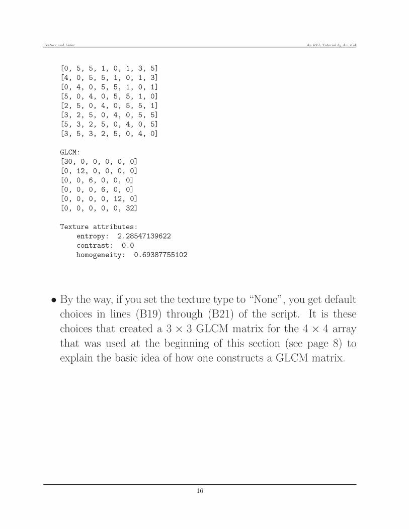
Texture type chosen: low_contrast
The image:
15
Texture and Color An RVL Tutorial by Avi Kak
[0, 5, 5, 1, 0, 1, 3, 5]
[4, 0, 5, 5, 1, 0, 1, 3]
[0, 4, 0, 5, 5, 1, 0, 1]
[5, 0, 4, 0, 5, 5, 1, 0]
[2, 5, 0, 4, 0, 5, 5, 1]
[3, 2, 5, 0, 4, 0, 5, 5]
[5, 3, 2, 5, 0, 4, 0, 5]
[3, 5, 3, 2, 5, 0, 4, 0]
GLCM:
[30, 0, 0, 0, 0, 0]
[0, 12, 0, 0, 0, 0]
[0, 0, 6, 0, 0, 0]
[0, 0, 0, 6, 0, 0]
[0, 0, 0, 0, 12, 0]
[0, 0, 0, 0, 0, 32]
Texture attributes:
entropy: 2.28547139622
contrast: 0.0
homogeneity: 0.69387755102
• By the way, if you set the texture type to “None”, you get default
choices in lines (B19) through (B21) of the script. It is these
choices that created a 3 × 3 GLCM matrix for the 4 × 4 array
that was used at the beginning of this section (see page 8) to
explain the basic idea of how one constructs a GLCM matrix.
16

Texture and Color An RVL Tutorial by Avi Kak
3.1: Summary of GLCM Properties
Here is a summary of the GLCM matrix properties:
• GLCM is of size M ×M for an image that has M different gray
levels.
• The matrix is symmetric
• Typically, one does NOT construct a GLCM matrix for the full
range of gray levels in an image. For 8-bit gray level images with
its 256 shades of gray (that is, the shade of brightness at each
pixel is an integer between 0 and 255, both ends inclusive), you
are likely to create a GLCM matrix of size of just 16 × 16 that
corresponds to a re-quantization of the gray levels to just 4 bits
(for the purpose of texture characterization).
• Also typically, one may construct multiple GLCM matrices forthe same image for different values of the displacement vectors.At the least, one uses the displacement vectors: (0, 1), (1, 0), and(1, 1). [These are the only three possible displacement vectors for a unit Chessboard Distance between
the reference pixel and the displaced pixel. (The Chessboard Distance gives us the number of moves requiredby the King piece in a chess game to get to a square from its current position on the board.) The Chessboard
17

Texture and Color An RVL Tutorial by Avi Kak
Distance, also known as the Chebyshev Distance or the L∞ norm, is equal to the max of the coordinate-wisedifferences between two points. The other distance you frequently run into in digital geometry is the Cityblockdistance, also known as the Manhattan or the Taxicab distance. The Cityblock Distance between any twopoints is the sum of the absolute differences of the cooordinates of the two points. More formally, the Cityblockdistance is referred to as the L1 norm. The 8 immediate neighbors of a pixel as shown at left below are at aChessboard Distance of 1 from the pixel. However, as shown at right below, only the two column-wise closestneighbors and the two row-wise closest neighbors of a pixel are at a Cityblock distance of 1:
X X X X
X P X X P X
X X X X
Neighbors at a unit Neighbors at a unit
Chessboard Distance of P Cityblock distance from P
(AKA Chebyshev Distance) (AKA Manhattan or Taxicab Dist.)
L_inf norm: ||x||_inf L_1 norm: ||x||_1
max of coord diffs sum of coord diffs
In and of itself, the GLCM characterization does not care what distance metric you use for the displacement
vector d.]
• To interpret a GLCM matrix as a joint probability distribution,
you need to normalize the matrix by dividing its individual ele-
ments by the sum of all the elements. That gives you a legiti-
mate joint (or bivariate) probability distribution over two random
variables that represent the gray levels at the two ends of the dis-
placement vector.
18

Texture and Color An RVL Tutorial by Avi Kak
3.2: Deriving Texture Measures from GLCM
• Each element of a GLCM matrix provides too “microscopic” a
view of a texture in an image. What we need is a larger “macro-
scopic” characterization of the texture from the information con-
tained in a GLCM matrix. [Let’s say you have constructed a 16× 16 GLCM
matrix (under the assumption that, regardless of the number of gray levels in an image,
you’ll place them in just 16 bins for the purpose of texture characterization). Each of
the 256 numbers in the GLCM matrix gives you a relative frequency of joint occurrence
of the two gray levels that corresponds to the row-column position of that element in
the matrix. Given these 256 GLCM numbers, what we need are a much smaller number
of numeric characterizations of the texture that can be derived from the GLCM matrix
numbers.]
• Perhaps the most popular characterization of the GLCM matrix
is through an entropy value that can be derived when the ma-
trix array is interpreted as a joint probability distribution. This
entropy is defined by:
Entropy = −M−1∑
i=0
M−1∑
j=0
P [i, j] log2 P [i, j] (2)
where P [i, j] is the normalized GLCM matrix. As mentioned at
the beginning of Section 3, P [i, j] is the joint probability distribu-
19

Texture and Color An RVL Tutorial by Avi Kak
tion of the gray levels at the two ends of the displacement vector
in the image.
• Regarding some properties of entropy that are important from
the standpoint of its use as a texture characterizer, it takes on its
maximum value when a probability distribution is uniform and
its minimum value of 0 when the probability distribution becomes
deterministic, meaning that when only a single cell in the GLCM
matrix is populated. [The probability distribution would be uniform for a completely random
texture. And the probability distribution would become deterministic when all of the gray levels in the image
are identical — that is, when there is no texture in the image.]
• Consider the case when the joint distribution is uniform: Given
a 16 × 16 GLCM matrix, we will have P [i, j] = 1/256. In this
case, the entropy is
Entropy = −15∑
i=0
15∑
j=0
1
256log2 2
−8
= −15∑
i=0
15∑
j=0
1
256(−8)
= 8.15∑
i=0
15∑
j=0
1
256
= 8 bits (3)
• So if you assign all of the gray levels in an image to 16 bins and
it turns out that the entropy calculated from the 16× 16 GLCM
20

Texture and Color An RVL Tutorial by Avi Kak
matrix is 8 bits, you have a completely random texture in the
image.
• Now consider the opposite case, that is, when an image has the
same gray level at all the pixels. In this case, only one cell of
the GLCM matrix would be populated — the cell at the [0, 0]
element of the matrix. By using the property that x · log x goes
to zero as x approaches 0, it is easy to show that the Entropy
becomes zero for this case.
• So, for images whose gray levels have been placed in 16 bins, we
have two bounds on the value of the entropy as derived from a
GLCM matrix: a maximum of 8 bits when the texture is com-
pletely random and a minimum of 0 when all the pixels have the
same gray level. For all other textures, the value of entropy will
be between these two bounds.
• The main rule to remember here is that the smaller the value of
the entropy the more nonuniform a GLCM matrix.
• Here are some other textures attributes that are derived from a
GLCM Matrix:
Energy =M−1∑
i=0
M−1∑
j=0
P [i, j]2
21

Texture and Color An RVL Tutorial by Avi Kak
Contrast =M−1∑
i=0
M−1∑
j=0
(i− j)2.P [i, j]
Homogeneity =
∑M−1i=0
∑M−1j=0 P [i, j]
1 + |i− j|(4)
• The first of these, Energy, is also called “Uniformity.” Its value
is the smallest when all the P [i, j] values are the same — that
is, for the case of a completely random texture. Note that since
P [i, j] must obey the unit summation constraint, if the values are
high for some values of i and j, they must be low elsewhere. In
the extreme case, only one cell will have the value P [i, j] equal to
1 and all other cells will be zero. For this extreme case, Energy
acquires the largest value of 1. At the other extreme, each cell
will have a value of 1/256 for the case a 16x16 GLCM matrix.
In this case, Energy will equal 256 × (1/256)2 = 1/256. For all
other cases of 16 × 16 GLCM matrices, Energy will range from
the low of 1/256 to the max of 1.
• Consider now the Contrast attribute of a texture defined in Eqs.
(4). This attribute takes on a low value when the values in the
GLCM matrix are large along and in the vicinity of the diagonal.
In the extreme case, if only the diagonal entries in the GLCM
matrix are populated, Contrast is 0. As you would expect, when
the displacement vector is (1, 1), the value of Contrast for an
22

Texture and Color An RVL Tutorial by Avi Kak
image that consists of diagonal stripes of constant gray values —
with each stripe possibly of a different gray — is zero. This should
explain the logic used for creating the low contrast texture
pattern in lines (B12) through (B17) of the Python script that is
shown in the next section.
• Finally, let’s talk about the Homogeneity attribute defined in
Equation (4). You can think of this attribute as being the oppo-
site of the Contrast attribute. Homogeneity takes a high value
when the GLCM matrix is populated mainly along the diago-
nal. So when Contrast is high, Homogeneity will be low and vice
versa. But note that the two are not opposites in the strict sense
of the word — since their definitions are not reciprocal. That is,
even though they are opposites loosely speaking, we can expect
both these attributes to provide non-redundant characterizations
of the GLCM matrix.
23

Texture and Color An RVL Tutorial by Avi Kak
3.3: Python Code for Experimenting withGLCM
Shown below is the code that was used to generate the GLCM results
you saw previously on pages 11 through 15 of this tutorial.
#!/usr/bin/env python
## GLCM.py
## Author: Avi Kak ([email protected])
## Date: September 26, 2016
## Changes on January 21, 2018:
##
## Code made Python 3 compliant
## This script was written as a teaching aid for the lecture on "Textures
## and Color" as a part of my class on Computer Vision at Purdue. This
## Python script demonstrates how the Gray Level Co-occurrence Matrix can
## be used for characterizing image textures.
## For educational purposes, this script generates five different types of
## textures -- you make the choice by uncommenting one of the statements in lines
## (A1) through (A5). You can also set the size of the image array and number
## of gray levels to use.
## The basic definition of GLCM:
##
## The (m,n)-th element of the matrix is the number of times
## the reference-pixel gray level is m and the displaced pixel
## is n. In order to create a symmetric matrix, when you
## increment glcm(m,n) because you found the reference pixel to
## be equal to m and the displaced pixel to be n, you also
## increment glcm(n,m).
##
## The main idea in creating a symmetric GLCM matrix is that
## you only care about the fact that the gray levels m and n
## occur together at the two ends of the displacement d and
## that you don’t care that one of the two appears at one
## specific end and the other at the other specific end.
24
Texture and Color An RVL Tutorial by Avi Kak
## HOW TO USE THIS SCRIPT:
##
## 1. Specify the texture type you want by uncommenting one of the lines (A1)
## through (A6)
##
## Note that if uncomment line (A6), that sets the image size to 4
## and the number of gray levels of 3 regardless of the choices you
## make in lines (A7) and (A8)
##
## 2. Set the image size in line (A7)
##
## 3. Set the number of gray levels in line (A8)
##
## 4. Set the displacement vector by uncommenting one of the lines (A9),
# (A10), or (A11). However, note that the "low_contrast" choice for
## the contrast type in line (A5) is low contrast only when the displacement
## vector is set as in line (A9).
import random
import math
import functools
## UNCOMMENT THE TEXTURE TYPE YOU WNT:
#texture_type = ’random’ #(A1)
texture_type = ’vertical’ #(A2)
#texture_type = ’horizontal’ #(A3)
#texture_type = ’checkerboard’ #(A4)
#texture_type = ’low_contrast’ #(A5)
#texture_type = None #(A6)
IMAGE_SIZE = 8 #(A7)
GRAY_LEVELS = 6 #(A8)
displacement = [1,1] #(A9)
#displacement = [1,0] #(A10)
#displacement = [0,1] #(A11)
image = [[0 for _ in range(IMAGE_SIZE)] for _ in range(IMAGE_SIZE)] #(B1)
if texture_type == ’random’: #(B2)
image = [[random.randint(0,GRAY_LEVELS-1)
for _ in range(IMAGE_SIZE)] for _ in range(IMAGE_SIZE)] #(B3)
elif texture_type == ’diagonal’: #(B4)
image = [[GRAY_LEVELS - 1 if (i+j)%2 == 0 else 0
for i in range(IMAGE_SIZE)] for j in range(IMAGE_SIZE)] #(B5)
elif texture_type == ’vertical’: #(B6)
image = [[GRAY_LEVELS - 1 if i%2 == 0 else 0
for i in range(IMAGE_SIZE)] for _ in range(IMAGE_SIZE)] #(B7)
elif texture_type == ’horizontal’: #(B8)
image = [[GRAY_LEVELS - 1 if j%2 == 0 else 0
for i in range(IMAGE_SIZE)] for j in range(IMAGE_SIZE)] #(B9)
elif texture_type == ’checkerboard’: #(B10)
image = [[GRAY_LEVELS - 1 if (i+j+1)%2 == 0 else 0
for i in range(IMAGE_SIZE)] for j in range(IMAGE_SIZE)] #(B11)
elif texture_type == ’low_contrast’: #(B12)
25
Texture and Color An RVL Tutorial by Avi Kak
image[0] = [random.randint(0,GRAY_LEVELS-1) for _ in range(IMAGE_SIZE)] #(B13)
for i in range(1,IMAGE_SIZE): #(B14)
image[i][0] = random.randint(0,GRAY_LEVELS-1) #(B15)
for j in range(1,IMAGE_SIZE): #(B16)
image[i][j] = image[i-1][j-1] #(B17)
else: #(B18)
image = [[2, 0, 1, 1],[0, 1, 2, 0],[1, 1, 1, 2],[0, 0, 1, 1]] #(B19)
IMAGE_SIZE = 4 #(B20)
GRAY_LEVELS = 3 #(B21)
# CALCULATE THE GLCM MATRIX:
print("Texture type chosen: %s" % texture_type) #(C1)
print("The image: ") #(C2)
for row in range(IMAGE_SIZE): print(image[row]) #(C3)
glcm = [[0 for _ in range(GRAY_LEVELS)] for _ in range(GRAY_LEVELS)] #(C4)
rowmax = IMAGE_SIZE - displacement[0] if displacement[0] else IMAGE_SIZE -1 #(C5)
colmax = IMAGE_SIZE - displacement[1] if displacement[1] else IMAGE_SIZE -1 #(C6)
for i in range(rowmax): #(C7)
for j in range(colmax): #(C8)
m, n = image[i][j], image[i + displacement[0]][j + displacement[1]] #(C9)
glcm[m][n] += 1 #(C10)
glcm[n][m] += 1 #(C11)
print("\nGLCM: ") #(C12)
for row in range(GRAY_LEVELS): print(glcm[row]) #(C13)
# CALCULATE ATTRIBUTES OF THE GLCM MATRIX:
entropy = energy = contrast = homogeneity = None #(D1)
normalizer = functools.reduce(lambda x,y: x + sum(y), glcm, 0) #(D2)
for m in range(len(glcm)): #(D3)
for n in range(len(glcm[0])): #(D4)
prob = (1.0 * glcm[m][n]) / normalizer #(D5)
if (prob >= 0.0001) and (prob <= 0.999): #(D6)
log_prob = math.log(prob,2) #(D7)
if prob < 0.0001: #(D8)
log_prob = 0 #(D9)
if prob > 0.999: #(D10)
log_prob = 0 #(D11)
if entropy is None: #(D12)
entropy = -1.0 * prob * log_prob #(D13)
continue #(D14)
entropy += -1.0 * prob * log_prob #(D15)
if energy is None: #(D16)
energy = prob ** 2 #(D17)
continue #(D18)
energy += prob ** 2 #(D19)
if contrast is None: #(D20)
contrast = ((m - n)**2 ) * prob #(D21)
continue #(D22)
contrast += ((m - n)**2 ) * prob #(D23)
26
Texture and Color An RVL Tutorial by Avi Kak
if homogeneity is None: #(D24)
homogeneity = prob / ( ( 1 + abs(m - n) ) * 1.0 ) #(D25)
continue #(D26)
homogeneity += prob / ( ( 1 + abs(m - n) ) * 1.0 ) #(D27)
if abs(entropy) < 0.0000001: entropy = 0.0 #(D28)
print("\nTexture attributes: ") #(D29)
print(" entropy: %f" % entropy) #(D30)
print(" contrast: %f" % contrast) #(D31)
print(" homogeneity: %f" % homogeneity) #(D32)
27

Texture and Color An RVL Tutorial by Avi Kak
4: CHARACTERIZING IMAGETEXTURES WITH LOCAL BINARYPATTERN (LBP) HISTOGRAMS
• Another way to create rotationally and gray-scale invariant char-
acterizations of image texture is by using Local Binary Pattern
(LBP) histograms. Such histograms are invariant to in-plane ro-
tations and to any monotonic transformations of the gray scale.
• The LBP method for characterizing textures was first introduced
by T. Ojala, M. Pietikainen, and T. Maenpaa in their paper “Mul-
tiresolution gray-scale and rotation invariant texture classification
with local binary patterns,” IEEE Transactions on Pattern Anal-
ysis and Machine Intelligence, vol. 24, no. 7, pp. 971-987, 2002.
• Fundamental to understating the idea of LBP is the notion of
a local binary pattern to characterize the gray level variations
around a pixel through runs of 0s and 1s. Experiments with
textures have shown that runs that consist of a single run of 0s
followed by a single run of 1s carry most of the discriminative
information between different kinds of textures.
28

Texture and Color An RVL Tutorial by Avi Kak
• The discussion that follows addresses the following different as-
pects of LBP:
– How to characterize the local inter-pixel variations in gray
levels by binary patterns in such a way that the patterns are
invariant to linear changes in image contrast;
– How to “reduce” a binary patterns resulting from the previous
step to their canonical forms that stay invariant to in-plane
rotations;
– And, how to focus on “uniform” patterns since they contain
most of the inter-texture discriminatory information and, sub-
sequently, how to create a histogram based characterization of
a texture.
29

Texture and Color An RVL Tutorial by Avi Kak
4.1: Characterizing a Local Inter-PixelGray-Level Variation by a
Contrast-Change-Invariant Binary Pattern
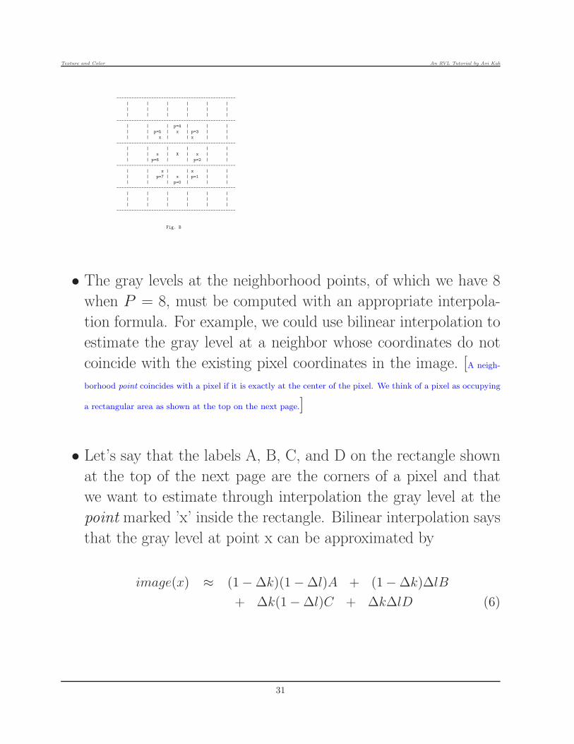
• Consider the pixel at the location marked by uppercase ’X’ in
Fig. A below and its 8 neighboring points on a unit circle. The
exact positions of the neighboring points vis-a-vis the pixel under
consideration is given by
(∆u,∆v) =
(
R cos (2πp
P), R sin (
2πp
P)
)
p = 0, 1, 2, .., 7 (5)
with the radius R = 1 and with P = 8. The point p = 0 gives us
the neighboring point that is straight down from the pixel under
consideration; the point p = 1, the neighboring point to the right
of the one that is straight down; and so on. Fig. B on the next
page shows the neighboring points for the different values of the
index p in the equation shown above..---> v
|
| ------------------------------------------------
V | | | | | |
u | | | | | |
| | | | | |
------------------------------------------------
| | | | | |
| | | x | | |
| | x | | x | |
------------------------------------------------
| | | | | |
| | x | X | x | |
| | | | | |
------------------------------------------------
| | x | | x | |
| | | x | | |
| | | | | |
------------------------------------------------
| | | | | |
| | | | | |
| | | | | |
------------------------------------------------
Fig. A
30
Texture and Color An RVL Tutorial by Avi Kak
------------------------------------------------
| | | | | |
| | | | | |
| | | | | |
------------------------------------------------
| | | p=4 | | |
| | p=5 | x | p=3 | |
| | x | | x | |
------------------------------------------------
| | | | | |
| | x | X | x | |
| | p=6 | | p=2 | |
------------------------------------------------
| | x | | x | |
| | p=7 | x | p=1 | |
| | | p=0 | | |
------------------------------------------------
| | | | | |
| | | | | |
| | | | | |
------------------------------------------------
Fig. B
• The gray levels at the neighborhood points, of which we have 8
when P = 8, must be computed with an appropriate interpola-
tion formula. For example, we could use bilinear interpolation to
estimate the gray level at a neighbor whose coordinates do not
coincide with the existing pixel coordinates in the image. [A neigh-
borhood point coincides with a pixel if it is exactly at the center of the pixel. We think of a pixel as occupying
a rectangular area as shown at the top on the next page.]
• Let’s say that the labels A, B, C, and D on the rectangle shown
at the top of the next page are the corners of a pixel and that
we want to estimate through interpolation the gray level at the
point marked ’x’ inside the rectangle. Bilinear interpolation says
that the gray level at point x can be approximated by
image(x) ≈ (1−∆k)(1−∆l)A + (1−∆k)∆lB
+ ∆k(1−∆l)C + ∆k∆lD (6)
31

Texture and Color An RVL Tutorial by Avi Kak
\Del l
--------->
.
A . B
--------------
| | . |
\Del k | | . |
| | . |
V | . |
.........|....... x |
| |
--------------
C D
• The bilinear interpolation formula is based on the assumption
that the inter-pixel sampling interval is a unit distance along the
horizontal and the vertical axes and that the location of ’x’ is a
fraction of unity as measured from point A.
• After estimating the gray levels at each of the P points on the
circle, we threshold these gray levels with respect to the gray level
value at the pixel at the center of the pixel. If the interpolated
value at a point is equal or greater than the value at the center,
we set that point to 1. Otherwise, we set it to 0.
• If (i, j) are the coordinates of the pixel at the center of the circle,
we now create our binary pattern around the circle through the
logic shown below:
pattern = []
for p in range(P):
image_val_at_p = interpolated value at point p on the circle
32

Texture and Color An RVL Tutorial by Avi Kak
if image_val_at_p >= image[i][j]:
pattern.append(1)
else:
pattern.append(0)
• Consider the following example:-------------------------
| | | |
| 1 | 5 | 3 |
| x | | x |
-------------------------
| | | |
| 5 | 3 | 1 |
| | | |
-------------------------
| x | | x |
| 4 | 0 | 0 |
| | | |
-------------------------
Fig. C
NOTE: ’x’ designates those locations on
the unit circle where the point does
not coincide with the pixel. Cells with
no ’x’ are those where the points on
the circle coincide with those on the
circle.
• Going around the central pixel where the gray level is 3, we start
with p=0 point on the unit-circle neighbors of this pixel. This is
the pixel just below the central pixel and the gray level there is 0.
The next point on circle, for p=1, does not coincide with a pixel.
This point is in the cell that belongs to the pixel whose gray level
is also 0. To find by bilinear interpolation the gray level at that
point, we see the following situation:
33

Texture and Color An RVL Tutorial by Avi Kak
0.707
--------->
.
3 . 1
--------------
| | . |
0.707 | | . |
| | . |
V | . |
.........|....... x |
| |
--------------
0 0
Fig. D
• Using the bilinear interpolation formula shown earlier, we esti-
mate the gray level at the point marked ’x’ as
3× (1− 0.707)× (1− 0.707) + 1× (1− 0.707)× 0.707 +
0× 0.707× (1− 0.707) + 0× 0.707× 0.707 = 0.464 (7)
• If we carry out similar calculations for each of the six remaining
points on the circle, we get the following 8 gray values on the
circle:
0.0 0.464 1.0 3.0 5.0 2.828 5.0 3.292
Thresholding these values by 3.0, the pixel value at the center of
the circle, gives us the binary pattern:
0 0 0 1 1 0 1 1
That brings us to the issue of how to make such binary patterns
invariant to in-plane rotations of the image.
34

Texture and Color An RVL Tutorial by Avi Kak
4.2: Generating Rotation-InvariantRepresentations from Local Binary Patterns
• Let’s say you are imaging a 2D textured surface, such as a brick
wall, under the condition that the sensor plane in your camera is
parallel to the surface. You have an in-plane rotation of the image
if you turn the camera while keeping its sensor plane parallel to
the textured surface. If the sampling rate in the image plane
is sufficiently high, as you rotate the camera, the digital images
would undergo corresponding rotations.
• Under the conditions described above, an in-plane rotation of an
image will cause the P points on a circular neighborhood to move
along the circle. We now need some way to characterize such a
binary pattern for all possible rotations. The original authors
of LBP proposed circularly rotating a binary pattern until the
largest number of 0’s occupy the most significant positions. This
is the same as circularly rotating a binary pattern until it acquires
the smallest integer value. We will refer to this representation of
a binary pattern as its minIntVal representation.
• In a Python implementation, the minIntVal form of a binary
pattern can easily be found by using my BitVector module. In
35
Texture and Color An RVL Tutorial by Avi Kak
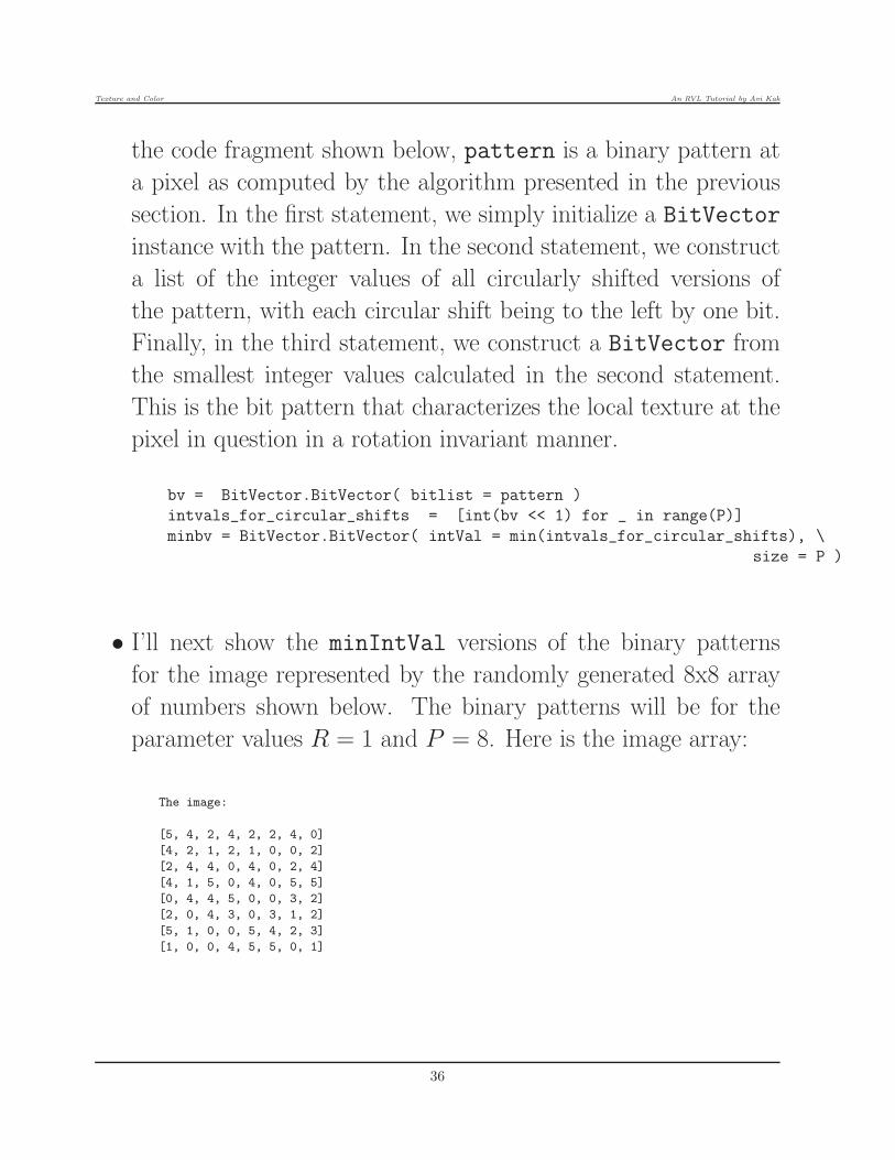
the code fragment shown below, pattern is a binary pattern at
a pixel as computed by the algorithm presented in the previous
section. In the first statement, we simply initialize a BitVector
instance with the pattern. In the second statement, we construct
a list of the integer values of all circularly shifted versions of
the pattern, with each circular shift being to the left by one bit.
Finally, in the third statement, we construct a BitVector from
the smallest integer values calculated in the second statement.
This is the bit pattern that characterizes the local texture at the
pixel in question in a rotation invariant manner.
bv = BitVector.BitVector( bitlist = pattern )
intvals_for_circular_shifts = [int(bv << 1) for _ in range(P)]
minbv = BitVector.BitVector( intVal = min(intvals_for_circular_shifts), \
size = P )
• I’ll next show the minIntVal versions of the binary patterns
for the image represented by the randomly generated 8x8 array
of numbers shown below. The binary patterns will be for the
parameter values R = 1 and P = 8. Here is the image array:
The image:
[5, 4, 2, 4, 2, 2, 4, 0]
[4, 2, 1, 2, 1, 0, 0, 2]
[2, 4, 4, 0, 4, 0, 2, 4]
[4, 1, 5, 0, 4, 0, 5, 5]
[0, 4, 4, 5, 0, 0, 3, 2]
[2, 0, 4, 3, 0, 3, 1, 2]
[5, 1, 0, 0, 5, 4, 2, 3]
[1, 0, 0, 4, 5, 5, 0, 1]
36
Texture and Color An RVL Tutorial by Avi Kak
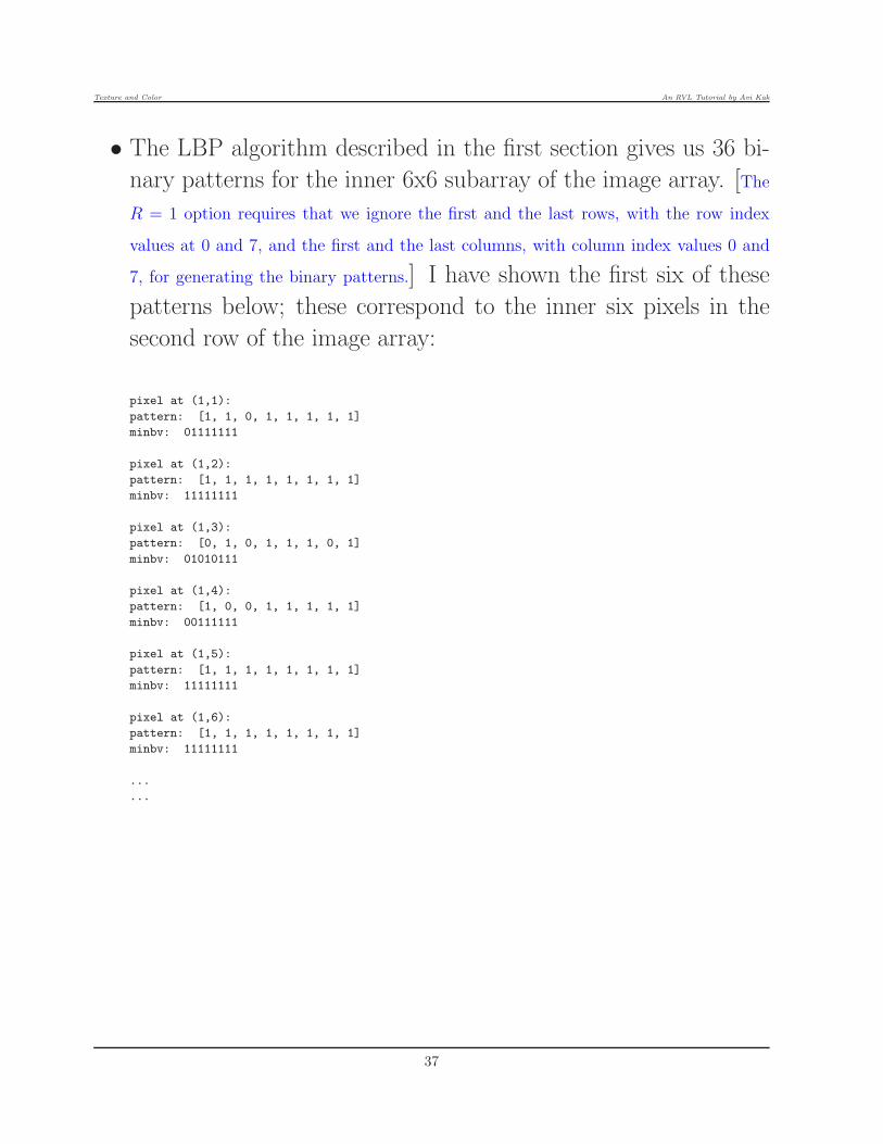
• The LBP algorithm described in the first section gives us 36 bi-
nary patterns for the inner 6x6 subarray of the image array. [The
R = 1 option requires that we ignore the first and the last rows, with the row index
values at 0 and 7, and the first and the last columns, with column index values 0 and
7, for generating the binary patterns.] I have shown the first six of these
patterns below; these correspond to the inner six pixels in the
second row of the image array:
pixel at (1,1):
pattern: [1, 1, 0, 1, 1, 1, 1, 1]
minbv: 01111111
pixel at (1,2):
pattern: [1, 1, 1, 1, 1, 1, 1, 1]
minbv: 11111111
pixel at (1,3):
pattern: [0, 1, 0, 1, 1, 1, 0, 1]
minbv: 01010111
pixel at (1,4):
pattern: [1, 0, 0, 1, 1, 1, 1, 1]
minbv: 00111111
pixel at (1,5):
pattern: [1, 1, 1, 1, 1, 1, 1, 1]
minbv: 11111111
pixel at (1,6):
pattern: [1, 1, 1, 1, 1, 1, 1, 1]
minbv: 11111111
...
...
37

Texture and Color An RVL Tutorial by Avi Kak
4.3: Encoding the minIntVal Forms of theLocal Binary Patterns
• Recall that each of the 36 minIntVal binary patterns shown
above represents only a pixel-based property, albeit one that is
rotationally invariant, of the local gray level variations in the
vicinity of that pixel. Our ultimate goal is to create an image-
based characterization of the texture.
• Toward that end, we now encode each minIntVal binary pattern
by a single integer. Since each such integer will represent the
local gray level variations at each pixel, a histogram of all such
encodings may subsequently be used to characterize the texture
in an image.
• That leads to the question as to what single integer encoding to
use for each minIntVal binary pattern.
• An obvious answer to this question is to use the integer value
of the patterns. For the case of P = 8 patterns, that would
mean associating an integer value between 0 and 127, both ends
inclusive, with each rotationally invariant minIntVal pattern.
Unfortunately, what speaks against this straightforward encod-
38

Texture and Color An RVL Tutorial by Avi Kak
ing of the patterns is the observation made by the creators of
LBP that generally only those minIntVal patterns are useful
for image-level characterization of a texture that consist of a sin-
gle run of 0’s followed by a single run of 1’s — assuming that a
pattern has both 0’s and 1’s. Such binary patterns were called
uniform by them.
• With that observation in mind, the creators of LBP have sug-
gested the following encodings for the patterns:
– If the minIntVal representation of a binary pattern has ex-
actly two runs, that is, a run of 0s followed by a run of 1s,
represent the pattern by the number of 1’s in the second run.
Such encodings would be integers between 1 and P − 1, both
ends inclusive.
– Else, if the minIntVal representation consists of all 0’s, rep-
resent it be the encoding 0.
– Else, if the minIntVal representation consists of all 1’s, rep-
resent it by the encoding P .
– Else, if the minIntVal representation involves more than two
runs, encode it by the integer P + 1.
• The encoding formula presented above requires that we first ex-
39
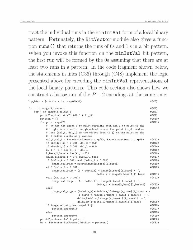
Texture and Color An RVL Tutorial by Avi Kak
tract the individual runs in the minIntVal form of a local binary
pattern. Fortunately, the BitVector module also gives a func-
tion runs() that returns the runs of 0s and 1’s in a bit pattern.
When you invoke this function on the minIntVal bit pattern,
the first run will be formed by the 0s assuming that there are at
least two runs in a pattern. In the code fragment shown below,
the statements in lines (C36) through (C48) implement the logic
presented above for encoding the minIntVal representations of
the local binary patterns. This code section also shows how we
construct a histogram of the P + 2 encodings at the same time:lbp_hist = {t:0 for t in range(P+2)} #(C6)
for i in range(R,rowmax): #(C7)
for j in range(R,colmax): #(C8)
print("\npixel at (%d,%d):" % (i,j)) #(C9)
pattern = [] #(C10)
for p in range(P): #(C11)
# We use the index k to point straight down and l to point to the
# right in a circular neighborhood around the point (i,j). And we
# use (del_k, del_l) as the offset from (i,j) to the point on the
# R-radius circle as p varies.
del_k,del_l = R*math.cos(2*math.pi*p/P), R*math.sin(2*math.pi*p/P) #(C12)
if abs(del_k) < 0.001: del_k = 0.0 #(C13)
if abs(del_l) < 0.001: del_l = 0.0 #(C14)
k, l = i + del_k, j + del_l #(C15)
k_base,l_base = int(k),int(l) #(C16)
delta_k,delta_l = k-k_base,l-l_base #(C17)
if (delta_k < 0.001) and (delta_l < 0.001): #(C18)
image_val_at_p = float(image[k_base][l_base]) #(C19)
elif (delta_l < 0.001): #(C20)
image_val_at_p = (1 - delta_k) * image[k_base][l_base] + \
delta_k * image[k_base+1][l_base] #(C21)
elif (delta_k < 0.001): #(C22)
image_val_at_p = (1 - delta_l) * image[k_base][l_base] + \
delta_l * image[k_base][l_base+1] #(C23)
else: #(C24)
image_val_at_p = (1-delta_k)*(1-delta_l)*image[k_base][l_base] + \
(1-delta_k)*delta_l*image[k_base][l_base+1] + \
delta_k*delta_l*image[k_base+1][l_base+1] + \
delta_k*(1-delta_l)*image[k_base+1][l_base] #(C25)
if image_val_at_p >= image[i][j]: #(C26)
pattern.append(1) #(C27)
else: #(C28)
pattern.append(0) #(C29)
print("pattern: %s" % pattern) #(C30)
bv = BitVector.BitVector( bitlist = pattern ) #(C31)
40

Texture and Color An RVL Tutorial by Avi Kak
intvals_for_circular_shifts = [int(bv << 1) for _ in range(P)] #(C32)
minbv = BitVector.BitVector( intVal = \
min(intvals_for_circular_shifts), size = P ) #(C33)
print("minbv: %s" % minbv) #(C34)
bvruns = minbv.runs() #(C35)
encoding = None
if len(bvruns) > 2: #(C36)
lbp_hist[P+1] += 1 #(C37)
encoding = P+1 #(C38)
elif len(bvruns) == 1 and bvruns[0][0] == ’1’: #(C39)
lbp_hist[P] += 1 #(C40)
encoding = P #(C41)
elif len(bvruns) == 1 and bvruns[0][0] == ’0’: #(C42)
lbp_hist[0] += 1 #(C43)
encoding = 0 #(C44)
else: #(C45)
lbp_hist[len(bvruns[1])] += 1 #(C46)
encoding = len(bvruns[1]) #(C47)
print("encoding: %s" % encoding) #(C48)
print("\nLBP Histogram: %s" % lbp_hist) #(C49)
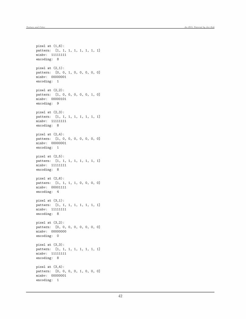
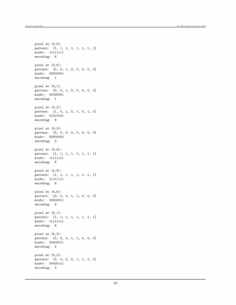
• Shown below are the encodings for the local binary patterns for
each of the inner 6x6 section of the 8x8 image array presented
towards the end of the previous subsection:
pixel at (1,1):
pattern: [1, 1, 0, 1, 1, 1, 1, 1]
minbv: 01111111
encoding: 7
pixel at (1,2):
pattern: [1, 1, 1, 1, 1, 1, 1, 1]
minbv: 11111111
encoding: 8
pixel at (1,3):
pattern: [0, 1, 0, 1, 1, 1, 0, 1]
minbv: 01010111
encoding: 9
pixel at (1,4):
pattern: [1, 0, 0, 1, 1, 1, 1, 1]
minbv: 00111111
encoding: 6
pixel at (1,5):
pattern: [1, 1, 1, 1, 1, 1, 1, 1]
minbv: 11111111
encoding: 8
41
Texture and Color An RVL Tutorial by Avi Kak
pixel at (1,6):
pattern: [1, 1, 1, 1, 1, 1, 1, 1]
minbv: 11111111
encoding: 8
pixel at (2,1):
pattern: [0, 0, 1, 0, 0, 0, 0, 0]
minbv: 00000001
encoding: 1
pixel at (2,2):
pattern: [1, 0, 0, 0, 0, 0, 1, 0]
minbv: 00000101
encoding: 9
pixel at (2,3):
pattern: [1, 1, 1, 1, 1, 1, 1, 1]
minbv: 11111111
encoding: 8
pixel at (2,4):
pattern: [1, 0, 0, 0, 0, 0, 0, 0]
minbv: 00000001
encoding: 1
pixel at (2,5):
pattern: [1, 1, 1, 1, 1, 1, 1, 1]
minbv: 11111111
encoding: 8
pixel at (2,6):
pattern: [1, 1, 1, 1, 0, 0, 0, 0]
minbv: 00001111
encoding: 4
pixel at (3,1):
pattern: [1, 1, 1, 1, 1, 1, 1, 1]
minbv: 11111111
encoding: 8
pixel at (3,2):
pattern: [0, 0, 0, 0, 0, 0, 0, 0]
minbv: 00000000
encoding: 0
pixel at (3,3):
pattern: [1, 1, 1, 1, 1, 1, 1, 1]
minbv: 11111111
encoding: 8
pixel at (3,4):
pattern: [0, 0, 0, 0, 1, 0, 0, 0]
minbv: 00000001
encoding: 1
42
Texture and Color An RVL Tutorial by Avi Kak
pixel at (3,5):
pattern: [1, 1, 1, 1, 1, 1, 1, 1]
minbv: 11111111
encoding: 8
pixel at (3,6):
pattern: [0, 0, 1, 0, 0, 0, 0, 0]
minbv: 00000001
encoding: 1
pixel at (4,1):
pattern: [0, 0, 1, 0, 0, 0, 0, 0]
minbv: 00000001
encoding: 1
pixel at (4,2):
pattern: [1, 0, 1, 0, 1, 0, 1, 0]
minbv: 01010101
encoding: 9
pixel at (4,3):
pattern: [0, 0, 0, 0, 0, 0, 0, 0]
minbv: 00000000
encoding: 0
pixel at (4,4):
pattern: [1, 1, 1, 1, 1, 1, 1, 1]
minbv: 11111111
encoding: 8
pixel at (4,5):
pattern: [1, 1, 1, 1, 1, 1, 1, 1]
minbv: 11111111
encoding: 8
pixel at (4,6):
pattern: [0, 0, 0, 1, 1, 0, 0, 0]
minbv: 00000011
encoding: 2
pixel at (5,1):
pattern: [1, 1, 1, 1, 1, 1, 1, 1]
minbv: 11111111
encoding: 8
pixel at (5,2):
pattern: [0, 0, 0, 1, 1, 0, 0, 0]
minbv: 00000011
encoding: 2
pixel at (5,3):
pattern: [0, 0, 0, 0, 1, 1, 1, 0]
minbv: 00000111
encoding: 3
43

Texture and Color An RVL Tutorial by Avi Kak
pixel at (5,4):
pattern: [1, 1, 1, 1, 1, 1, 1, 1]
minbv: 11111111
encoding: 8
pixel at (5,5):
pattern: [1, 0, 0, 0, 0, 0, 0, 1]
minbv: 00000011
encoding: 2
pixel at (5,6):
pattern: [1, 1, 1, 1, 1, 1, 1, 1]
minbv: 11111111
encoding: 8
pixel at (6,1):
pattern: [0, 0, 0, 1, 0, 1, 1, 1]
minbv: 00010111
encoding: 9
pixel at (6,2):
pattern: [1, 1, 1, 1, 1, 1, 1, 1]
minbv: 11111111
encoding: 8
pixel at (6,3):
pattern: [1, 1, 1, 1, 1, 1, 1, 1]
minbv: 11111111
encoding: 8
pixel at (6,4):
pattern: [1, 0, 0, 0, 0, 0, 0, 0]
minbv: 00000001
encoding: 1
pixel at (6,5):
pattern: [1, 0, 0, 0, 0, 0, 1, 1]
minbv: 00000111
encoding: 3
pixel at (6,6):
pattern: [0, 0, 1, 1, 0, 1, 1, 1]
minbv: 00110111
encoding: 9
LBP Histogram: {0: 2, 1: 6, 2: 3, 3: 2, 4: 1, 5: 0, 6: 1, 7: 1, 8: 15, 9: 5}
• Subsequently, when we construct a histogram over the P + 2
encodings of the patterns, we get the following result for the
44

Texture and Color An RVL Tutorial by Avi Kak
random 8x8 image array shown earlier:
LBP Histogram: {0: 3, 1: 5, 2: 1, 3: 0, 4: 0, 5: 1, 6: 4, 7: 3, 8: 19}
• Shown below are the LBP histograms for the other cases of tex-
tures you can produce with the LBP.py script that is presented
in the next subsection.
Texture type: vertical
[5, 0, 5, 0, 5, 0, 5, 0]
[5, 0, 5, 0, 5, 0, 5, 0]
[5, 0, 5, 0, 5, 0, 5, 0]
[5, 0, 5, 0, 5, 0, 5, 0]
[5, 0, 5, 0, 5, 0, 5, 0]
[5, 0, 5, 0, 5, 0, 5, 0]
[5, 0, 5, 0, 5, 0, 5, 0]
[5, 0, 5, 0, 5, 0, 5, 0]
LBP Histogram: {0: 0, 1: 0, 2: 0, 3: 0, 4: 0, 5: 0, 6: 0, 7: 0, 8: 18, 9: 18}
Texture type:: horizontal
[5, 5, 5, 5, 5, 5, 5, 5]
[0, 0, 0, 0, 0, 0, 0, 0]
[5, 5, 5, 5, 5, 5, 5, 5]
[0, 0, 0, 0, 0, 0, 0, 0]
[5, 5, 5, 5, 5, 5, 5, 5]
[0, 0, 0, 0, 0, 0, 0, 0]
[5, 5, 5, 5, 5, 5, 5, 5]
[0, 0, 0, 0, 0, 0, 0, 0]
LBP Histogram: {0: 0, 1: 0, 2: 0, 3: 0, 4: 0, 5: 0, 6: 0, 7: 0, 8: 18, 9: 18}
Texture type chosen: checkerboard
45

Texture and Color An RVL Tutorial by Avi Kak
[0, 5, 0, 5, 0, 5, 0, 5]
[5, 0, 5, 0, 5, 0, 5, 0]
[0, 5, 0, 5, 0, 5, 0, 5]
[5, 0, 5, 0, 5, 0, 5, 0]
[0, 5, 0, 5, 0, 5, 0, 5]
[5, 0, 5, 0, 5, 0, 5, 0]
[0, 5, 0, 5, 0, 5, 0, 5]
[5, 0, 5, 0, 5, 0, 5, 0]
LBP Histogram: {0: 18, 1: 0, 2: 0, 3: 0, 4: 0, 5: 0, 6: 0, 7: 0, 8: 18, 9: 0}
46

Texture and Color An RVL Tutorial by Avi Kak
4.4: Python Code for Experimenting withLBP
All of the LBP based results shown earlier were produced by the
Python script shown below.
The script generates elementary textures for you and applies the LBP
algorithm to the textures. You can specify the texture you want by
uncommenting one of lines in (A1) through (A5).
The script allows you to set any arbitrary size for the image array
and the number of gray levels you want in the image.
The script also allows you to give whatever values you wish to the P
and R parameters needed by the LBP algorithm.
#!/usr/bin/env python
## LBP.py
## Author: Avi Kak ([email protected])
## Date: November 1, 2016
## Changes on January 21, 2018:
##
## Code made Python 3 compliant
## This script was written as a teaching aid for the lecture on "Textures and Color"
## as a part of my class on Computer Vision at Purdue.
##
## This Python script demonstrates how Local Binary Patterns can be used for
## characterizing image textures.
## For educational purposes, this script generates five different types of textures
## -- you make the choice by uncommenting one of the statements in lines (A1)
47

Texture and Color An RVL Tutorial by Avi Kak
## through (A5). You can also set the size of the image array and number of gray
## levels to use.
## HOW TO USE THIS SCRIPT:
##
## 1. Specify the texture type you want by uncommenting one of the lines (A1)
## through (A5)
##
## 2. Set the image size in line (A6)
##
## 3. Set the number of gray levels in line (A7)
##
## 4. Choose a value for the circle radius R in line (A8)
#3
## 5. Choose a value for the number of sampling points on the circle in line (A9).
## Calling syntax: LBP.py
import random
import math
import BitVector
## UNCOMMENT THE TEXTURE TYPE YOU WANT:
#texture_type = ’random’ #(A1)
texture_type = ’vertical’ #(A2)
#texture_type = ’horizontal’ #(A3)
#texture_type = ’checkerboard’ #(A4)
#texture_type = None #(A5)
IMAGE_SIZE = 8 #(A6)
#IMAGE_SIZE = 4 #(A6)
GRAY_LEVELS = 6 #(A7)
R = 1 # the parameter R is radius of the circular pattern #(A8)
P = 8 # the number of points to sample on the circle #(A9)
image = [[0 for _ in range(IMAGE_SIZE)] for _ in range(IMAGE_SIZE)] #(B1)
if texture_type == ’random’: #(B2)
image = [[random.randint(0,GRAY_LEVELS-1)
for _ in range(IMAGE_SIZE)] for _ in range(IMAGE_SIZE)] #(B3)
elif texture_type == ’diagonal’: #(B4)
image = [[GRAY_LEVELS - 1 if (i+j)%2 == 0 else 0
for i in range(IMAGE_SIZE)] for j in range(IMAGE_SIZE)] #(B5)
elif texture_type == ’vertical’: #(B6)
image = [[GRAY_LEVELS - 1 if i%2 == 0 else 0
for i in range(IMAGE_SIZE)] for _ in range(IMAGE_SIZE)] #(B7)
elif texture_type == ’horizontal’: #(B8)
image = [[GRAY_LEVELS - 1 if j%2 == 0 else 0
for i in range(IMAGE_SIZE)] for j in range(IMAGE_SIZE)] #(B9)
elif texture_type == ’checkerboard’: #(B10)
image = [[GRAY_LEVELS - 1 if (i+j+1)%2 == 0 else 0
for i in range(IMAGE_SIZE)] for j in range(IMAGE_SIZE)] #(B11)
else: #(B12)
image = [[1, 5, 3, 1],[5, 3, 1, 4],[4, 0, 0, 0],[2, 3, 4, 5]] #(B13)
48

Texture and Color An RVL Tutorial by Avi Kak
IMAGE_SIZE = 4 #(B14)
GRAY_LEVELS = 3 #(B15)
print("Texture type chosen: %s" % texture_type) #(C1)
print("The image: ") #(C2)
for row in range(IMAGE_SIZE): print(image[row]) #(C3)
lbp = [[0 for _ in range(IMAGE_SIZE)] for _ in range(IMAGE_SIZE)] #(C4)
rowmax,colmax = IMAGE_SIZE-R,IMAGE_SIZE-R #(C5)
lbp_hist = {t:0 for t in range(P+2)} #(C6)
for i in range(R,rowmax): #(C7)
for j in range(R,colmax): #(C8)
print("\npixel at (%d,%d):" % (i,j)) #(C9)
pattern = [] #(C10)
for p in range(P): #(C11)
# We use the index k to point straight down and l to point to the
# right in a circular neighborhood around the point (i,j). And we
# use (del_k, del_l) as the offset from (i,j) to the point on the
# R-radius circle as p varies.
del_k,del_l = R*math.cos(2*math.pi*p/P), R*math.sin(2*math.pi*p/P) #(C12)
if abs(del_k) < 0.001: del_k = 0.0 #(C13)
if abs(del_l) < 0.001: del_l = 0.0 #(C14)
k, l = i + del_k, j + del_l #(C15)
k_base,l_base = int(k),int(l) #(C16)
delta_k,delta_l = k-k_base,l-l_base #(C17)
if (delta_k < 0.001) and (delta_l < 0.001): #(C18)
image_val_at_p = float(image[k_base][l_base]) #(C19)
elif (delta_l < 0.001): #(C20)
image_val_at_p = (1 - delta_k) * image[k_base][l_base] + \
delta_k * image[k_base+1][l_base] #(C21)
elif (delta_k < 0.001): #(C22)
image_val_at_p = (1 - delta_l) * image[k_base][l_base] + \
delta_l * image[k_base][l_base+1] #(C23)
else: #(C24)
image_val_at_p = (1-delta_k)*(1-delta_l)*image[k_base][l_base] + \
(1-delta_k)*delta_l*image[k_base][l_base+1] + \
delta_k*delta_l*image[k_base+1][l_base+1] + \
delta_k*(1-delta_l)*image[k_base+1][l_base] #(C25)
if image_val_at_p >= image[i][j]: #(C26)
pattern.append(1) #(C27)
else: #(C28)
pattern.append(0) #(C29)
print("pattern: %s" % pattern) #(C30)
bv = BitVector.BitVector( bitlist = pattern ) #(C31)
intvals_for_circular_shifts = [int(bv << 1) for _ in range(P)] #(C32)
minbv = BitVector.BitVector( intVal = \
min(intvals_for_circular_shifts), size = P ) #(C33)
print("minbv: %s" % minbv) #(C34)
bvruns = minbv.runs() #(C35)
encoding = None
if len(bvruns) > 2: #(C36)
lbp_hist[P+1] += 1 #(C37)
encoding = P+1 #(C38)
elif len(bvruns) == 1 and bvruns[0][0] == ’1’: #(C39)
49

Texture and Color An RVL Tutorial by Avi Kak
lbp_hist[P] += 1 #(C40)
encoding = P #(C41)
elif len(bvruns) == 1 and bvruns[0][0] == ’0’: #(C42)
lbp_hist[0] += 1 #(C43)
encoding = 0 #(C44)
else: #(C45)
lbp_hist[len(bvruns[1])] += 1 #(C46)
encoding = len(bvruns[1]) #(C47)
print("encoding: %s" % encoding) #(C48)
print("\nLBP Histogram: %s" % lbp_hist) #(C49)
50

Texture and Color An RVL Tutorial by Avi Kak
5: CHARACTERIZING IMAGETEXTURES WITH A GABOR FILTER
FAMILY
• Gabor filters are spatially localized operators for analyzing an
image for periodicities at different frequencies and in different
directions. To the extent that many image textures are composed
of repetitively occurring micro-patterns, that makes them ideal
for characterization by Gabor filters.
• You can think of a Gabor filter as a highly localized Fourier trans-
form in which the localization is achieved by applying a Gaussian
decay function to the pixels. Whereas the Gaussian weighting
gives us the localization needed, the direction of the periodici-
ties in the underlying Fourier kernel allows us to characterize a
texture in that direction.
• To underscore the importance of Gabor filters for texture char-
acterization, it is a part of the MPEG-7 multimedia content de-
scription standard. The standard specifies description formats for
the different components of multi-media objects such as audio,
images, and video. It is meant to be used as a complement to the
MPEG-4 standard whose primary focus is the standardization of
51

Texture and Color An RVL Tutorial by Avi Kak
compression routines for multi-media objects. The Gabor filter
based texture characterization in MPEG-7 is meant to facilitate
image search and retrieval. [The other two MPEG standards in current use are MPEG-1
and MPEG-2, both concerned primarily with the image resolution to be made available in a video service.
MPEG-1, which is the oldest such standard, specifies an image resolution of 352 × 240 at 30 fps (frames per
second). On the other hand, MPEG-2 specifies two image resolutions, 720 × 480 and 1280 × 720, both at 60
fps. The acronym MPEG stands for “Moving Picture Experts Group”. MPEG is a part of ISO (International
Organization for Standardization).]
• The Gabor filter as used in MPEG-7 makes 30 measurements on
a texture. These consist of 6 orientations and 5 spatial frequency
bands, as shown in the figure on the next page.
• Don’t worry if the precise meaning of the figure on the next page
is not clear at this time. The explanation that follows will explain
what is meant by the frequencies and the frequency bands in the
figure and also what we mean by the orientations of a Gabor
filter.
• Suffice it to say at the moment that if f0 is the frequency asso-
ciated with the outermost band of frequencies in the figure, the
other frequency band boundaries are given by
fs =f02s
s = 0, 1, 2, 3, 4 (8)
where s = 0 obviously corresponds to the outer boundary of the
52

Texture and Color An RVL Tutorial by Avi Kak
Figure 1: Defining the Gabor texture channels for the MPEG-7 stan-
dard by dividing the spatial frequencies in polar coordinates. The Ga-bor filter bank in this case consists of Gabor convolutional operatorsat 6 orientations and 5 spatial frequencies.
53

Texture and Color An RVL Tutorial by Avi Kak
outermost band. Note that, except for the lowest band, each
band represents an octave (since the upper limit of frequencies
in each band is twice the lower limit). Here are the frequency
bandwidths for the five different bands:
band1 =
(
f02, f0
)
band2 =
(
f04,f02
)
band3 =
(
f08,f04
)
band4 =
(
f016
,f08
)
band5 =
(
0,f016
)
• In what follows, I will start with a brief review of the 2D Fourier
transform.
54
Texture and Color An RVL Tutorial by Avi Kak
5.1: A Brief Review of 2D Fourier Transform
• Let’s start with the expression for the 2D Fourier transform of
an image:
G(u, v) =∫ ∞
x=−∞
∫ ∞
y=−∞g(x, y)e−j2π(ux+vy)dxdy (9)
and its inverse Fourier transform:
g(x, y) =∫ ∞
−∞G(u, v)ej2π(ux+vy)dudv (10)
• If we assume that our image consists of a single sinusoidal wave
that exhibits a periodicity of u0 cycles per unit length along the
x-axis and v0 cycles per unit length along the y-axis, then
G(u, v) = δ(u− u0, v − v0) (11)
where δ(u, v) is a dirac delta function that is non-zero only at
the point (u0, v0) in the (u, v)-plane. As is to be expected, the
image g(x, y) for such a G(u, v) would be given by
g(x, y) = ej2π(u0x+v0y)
= cos
(
2π(u0x + v0y)
)
+ j sin
(
2π(u0x+ v0y)
)
(12)
55

Texture and Color An RVL Tutorial by Avi Kak
The real part (and also the imaginary part) of the expression on
the right above is a two-dimensional sinusoidal wave (think of an
ocean wave) in the (x, y) plane that cuts the x-axis at u-cycles
per unit length and the y-axis at v cycles per unit length.
• As mentioned above, in the Fourier transform G(u, v), u is the
frequency of the 2D sinusoid as seen along the x-axis and v the
frequency of the same along the y-axis. The frequency along the
direction in the (x, y) plane along which the sinusoid changes
more rapidly (in terms of cycles per unit length) is given by
f =√u2 + v2 (13)
and the direction θ of the maximum rate of change is given by
the angle
θ = arctan(v/u) (14)
that is subtended with the x-axis. If we wish, we can express the
frequency components u and v in polar coordinates:
u = f ∗ cos(θ)v = f ∗ sin(θ) (15)
• In the polar representation of the frequencies, the formula for the
Fourier transform shown at the beginning of this section can be
expressed as
G(f, θ) =∫ ∞
r=0
∫ 2π
θ=0g(x, y)e−j2πf(x cos(θ)+y sin(θ))dxdy (16)
56
Texture and Color An RVL Tutorial by Avi Kak
5.2: The Gabor Filter Operator
• The convolutional operator for the continuous form a Gabor filter
is given by:
h(x, y; u, v) =1√πσ
e−x2+y2
2σ2 e−j2π(ux+vy) (17)
where u is the spatial frequency along x and v is the spatial
frequency along y. That is, if you looked at only those points of
h(x, y; u, v) that are on the x-axis, you will see a sinusoid with a
frequency of u cycles per unit length. And, if you did the same
along the y-axis, you will see a sinusoid with a frequency of v
cycles per unit length.
• Being a convolutional operator, we slide it to each pixel in the
image f(x,y), flip it with respect to the x and the y axes, multiply
the gray-level values at the pixels with the corresponding values
in the above operator and integrate the products:
g(x, y; u, v) =∫ ∞
−∞
∫ ∞
−∞f(α, β)h(x− α, y − β; u, v)dαdβ (18)
• If you substitute the expression for h(x, y; u, v) in the above equa-
tion — but without the exponential decay term — what you’ll
57
Texture and Color An RVL Tutorial by Avi Kak
get will be the same as the 2D Fourier transform (except for a
phase shift at each of the frequencies).
• What that implies is that the best way to interpret the Gabor
operator is to think of it as a localized Fourier transform of an
image where, for the calculation at each locale in the image, you
weight the pixels away from the locale according to the exponen-
tial decay factor. Obviously, the decay rate with respect to the
pixel coordinates is controlled by the ”standard deviation” σ
• What is interesting is that this Gaussian weighting in the space
domain results in Gaussian weighting in the frequency domain.
To see this, the Fourier transform of
h(x, y; u0, v0) =1
√
(π)σe−
1
2
x2+y2
2σ2 e−j2π(u0x+v0y) (19)
is given by
H(u, v; x, y) =σ2
2e−πσ2((u−u0)
2+(v−v0)2)ej2π(u0x+v0y) (20)
• What that shows is that each Gabor operator involves a band
of frequencies around the central frequency (u0, v0) of the filter
operator. The width of this frequency band is inversely propor-
tional to the width of the space domain operator. This should
clarify by what it means to create a Gabor filter for each of the
30 “channels” shown earlier in Fig. 1 for how the Gabor filter is
used in MPEG-7 (see page 53).
58

Texture and Color An RVL Tutorial by Avi Kak
• With regard to its implementation, it is more common to express
the Gabor filter operator in terms of the polar coordinates in the
frequency domain.
h(x, y; f, θ) =1√πσ
e−1
2
x2+y2
2σ2 e−j2πf(x cos(θ)+y sin(θ)) (21)
• To remind the reader, when we convolve an image g(x, y) with
this operator, at each pixel we will find the component of the
localized Gaussian weighted Fourier transform at the frequency f
along the direction given by θ with respect to the x axis. The form
shown above can be broken into the real part and the imaginary
part:
hre(x, y; f, θ) =1√πσ
e−1
2
x2+y2
2σ2 cos
(
2πf(x cos(θ) + y sin(θ))
)
him(x, y; f, θ) =1√πσ
e−1
2
x2+y2
2σ2 sin
(
2πf(x cos(θ) + y sin(θ))
)
(22)
For discrete implementation, we can represent the real and the
imaginary parts as
hre(i, j; f, θ) =1√πσ
e−1
2
i2+j2
2σ2 cos
(
2πf(i cos(θ) + j sin(θ))
)
him(i, j; f, θ) =1√πσ
e−1
2
i2+j2
2σ2 sin
(
2πf(i cos(θ) + j sin(θ))
)
(23)
where i represents the row index and the j the column index.
Note that we commonly think of the x-axis as being along the
59

Texture and Color An RVL Tutorial by Avi Kak
horizontal, going from left to right, and the y-axis as being along
the vertical, going from bottom to top. However, in the discrete
version, we think of the i index as representing the rows (that is, i
is along the vertical, going from top to bottom, and j is along the
horizontal, going from left to right. The origin in the continuous
case is usually at the center of the (x, y) plane. The origin in the
discrete case is at the upper left corner.
• An important issue for the discrete case is how far one should go
from the origin for a given value of σ. Obviously, the smaller the
value of σ, the faster the drop-off in terms of the weighting given
to the pixels in the image, and, therefore, the smaller the effec-
tive footprint of the operator on the (x, y) plane. A commonly
used rule of thumb for the discrete case is to let i and j cover a
bounding box that goes from −int(3σ) to int(3σ) along the x
and the y axes.
• As to purpose played by the coefficient
1√πσ
(24)
its purpose is to ensure that the “energy” of the operator is unity.
For the continuous case, the energy constraint is defined as
∫ ∞x=−∞
∫ ∞y=−∞ |h(x, y)|2 = 1 (25)
For the discrete case, you’d hopefully get a good approximation
60

Texture and Color An RVL Tutorial by Avi Kak
to the constraint with the summation shown below:
int(3σ)∑
i=−int(3σ)
int(3σ)∑
j=−int(3σ)|h(i, j)|2 ≈ 1 (26)
• The next subsection presents a Python script, Gabor.py, that
first generates a Gabor filter bank and then applies it to some
internally created image arrays. In that script, the basic Gabor
operator is defined by the function gabor() that is reproduced
below. As you can see, the statements in lines (B12) and (B13)
correspond to the two definitions shown previously in Eq. (23).
def gabor(sigma, theta, f, size): #(B1)
assert size >= 6 * sigma, \
"\n\nThe size of the Gabor operator must be at least 6 times sigma" #(B2)
W = size # Gabor operator Window width #(B3)
coef = 1.0 / (math.sqrt(math.pi) * sigma) #(B4)
ivals = range(-(W//2), W//2+1) #(B5)
jvals = range(-(W//2), W//2+1) #(B6)
greal = [[0.0 for _ in jvals] for _ in ivals] #(B7)
gimag = [[0.0 for _ in jvals] for _ in ivals] #(B8)
energy = 0.0 #(B9)
for i in ivals: #(B10)
for j in jvals: #(B11)
greal[i][j] = coef * math.exp(-((i**2 + j**2)/(2.0*sigma**2))) *\
math.cos(2*math.pi*(f/(1.0*W))*(i*math.cos(theta) +
j * math.sin(theta))) #(B12)
gimag[i][j] = coef * math.exp(-((i**2 + j**2)/(2.0*sigma**2))) *\
math.sin(2*math.pi*(f/(1.0*W))*(i*math.cos(theta) +
j * math.sin(theta))) #(B13)
energy += greal[i][j] ** 2 + gimag[i][j] ** 2 #(B14)
normalizer_r = functools.reduce(lambda x,y: x + sum(y), greal, 0) #(B15)
normalizer_i = functools.reduce(lambda x,y: x + sum(y), gimag, 0) #(B16)
print("\nnormalizer for the real part: %f" % normalizer_r) #(B17)
print("normalizer for the imaginary part: %.10f" % normalizer_i) #(B18)
print("energy: %f" % energy) #(B19)
return (greal, gimag) #(B20)
61

Texture and Color An RVL Tutorial by Avi Kak
• In the Gabor.py script in the next subsection, the function shown
above is used to create a bank of Gabor filters using the function
shown below:
def generate_filter_bank(sigma, size, how_many_frequencies,
how_many_directions): #(C1)
filter_bank = {f : {d : None for d in range(how_many_directions)}
for f in range(how_many_frequencies)} #(C2)
for freq in range(1,how_many_frequencies): #(C3)
for direc in range(how_many_directions): #(C4)
filter_bank[freq][direc] = \
gabor(sigma, direc*math.pi/how_many_directions, 2*freq, size) #(C5)
return filter_bank #(C6)
• In the function shown above, note the multiplier 2 for the vari-
able freq and the multiplier π/how many directions. So if
we choose 3 for how many frequencies, we will be testing the
periodicities at 2, 4, 6 cycles per window width. Similarly, if
we choose 4 for how many directions, we will be choosing the
angles 0, π/4, π/2, and 3π/4 for the directions.
• The two function defined above, gabor() and generate filter bank(),
generate the convolutional operators presented in the figure shown
below. As you can see, the rows in the figure are paired, with the
fist row in each pair for the real part of the Gabor convolutional
operator and the second row for the imaginary part. The first
two rows are for the spatial frequency of 2 cycles per operator
width; the next two rows for 4 cycles per operator width; and
the bottom two rows for 6 cycles per operator width. The four
columns stand for the four spatial directions of the operator as
listed in the previous bullet.
62
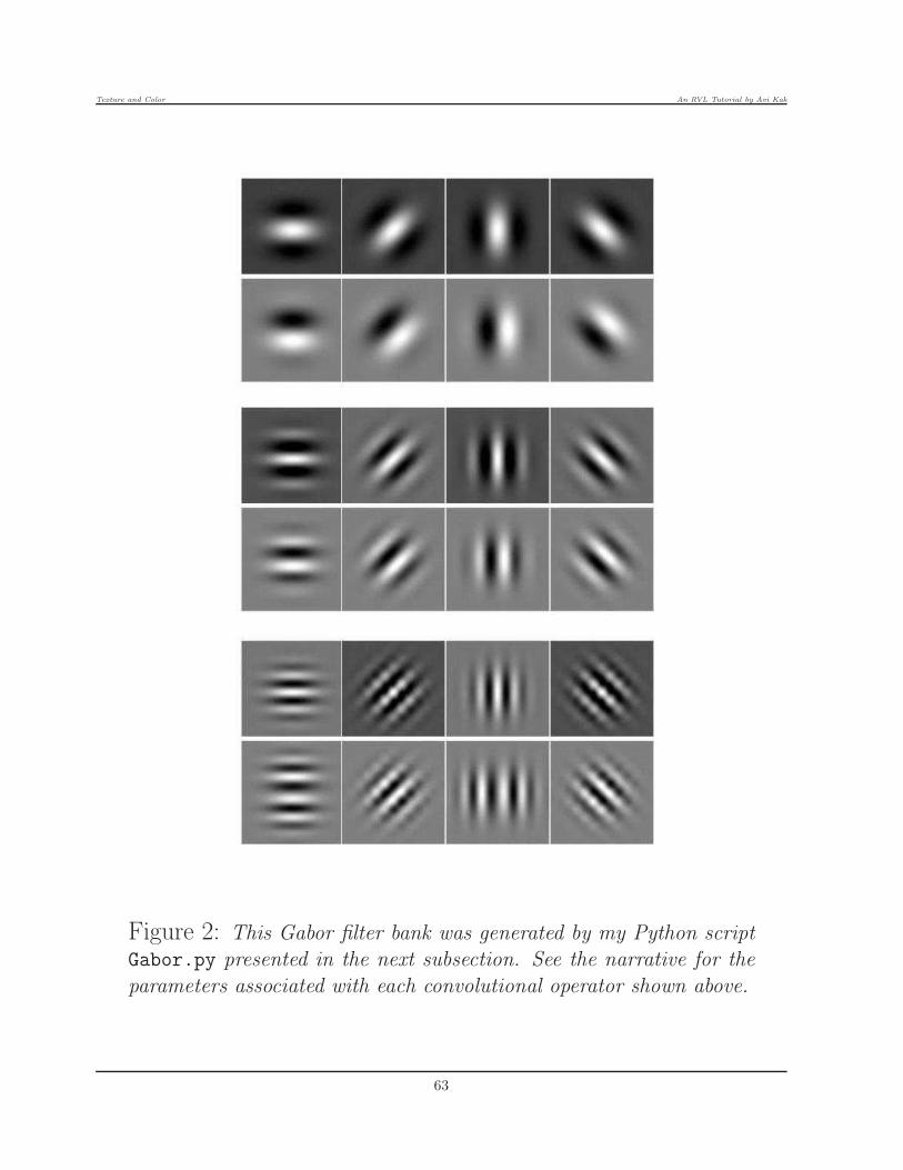
Texture and Color An RVL Tutorial by Avi Kak
Figure 2: This Gabor filter bank was generated by my Python scriptGabor.py presented in the next subsection. See the narrative for the
parameters associated with each convolutional operator shown above.
63
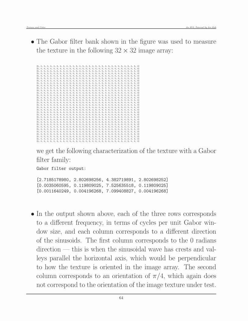
Texture and Color An RVL Tutorial by Avi Kak
• The Gabor filter bank shown in the figure was used to measure
the texture in the following 32× 32 image array:
[5, 0, 5, 0, 5, 0, 5, 0, 5, 0, 5, 0, 5, 0, 5, 0, 5, 0, 5, 0, 5, 0, 5, 0, 5, 0, 5, 0, 5, 0, 5, 0]
[5, 0, 5, 0, 5, 0, 5, 0, 5, 0, 5, 0, 5, 0, 5, 0, 5, 0, 5, 0, 5, 0, 5, 0, 5, 0, 5, 0, 5, 0, 5, 0]
[5, 0, 5, 0, 5, 0, 5, 0, 5, 0, 5, 0, 5, 0, 5, 0, 5, 0, 5, 0, 5, 0, 5, 0, 5, 0, 5, 0, 5, 0, 5, 0]
[5, 0, 5, 0, 5, 0, 5, 0, 5, 0, 5, 0, 5, 0, 5, 0, 5, 0, 5, 0, 5, 0, 5, 0, 5, 0, 5, 0, 5, 0, 5, 0]
[5, 0, 5, 0, 5, 0, 5, 0, 5, 0, 5, 0, 5, 0, 5, 0, 5, 0, 5, 0, 5, 0, 5, 0, 5, 0, 5, 0, 5, 0, 5, 0]
[5, 0, 5, 0, 5, 0, 5, 0, 5, 0, 5, 0, 5, 0, 5, 0, 5, 0, 5, 0, 5, 0, 5, 0, 5, 0, 5, 0, 5, 0, 5, 0]
[5, 0, 5, 0, 5, 0, 5, 0, 5, 0, 5, 0, 5, 0, 5, 0, 5, 0, 5, 0, 5, 0, 5, 0, 5, 0, 5, 0, 5, 0, 5, 0]
[5, 0, 5, 0, 5, 0, 5, 0, 5, 0, 5, 0, 5, 0, 5, 0, 5, 0, 5, 0, 5, 0, 5, 0, 5, 0, 5, 0, 5, 0, 5, 0]
[5, 0, 5, 0, 5, 0, 5, 0, 5, 0, 5, 0, 5, 0, 5, 0, 5, 0, 5, 0, 5, 0, 5, 0, 5, 0, 5, 0, 5, 0, 5, 0]
[5, 0, 5, 0, 5, 0, 5, 0, 5, 0, 5, 0, 5, 0, 5, 0, 5, 0, 5, 0, 5, 0, 5, 0, 5, 0, 5, 0, 5, 0, 5, 0]
[5, 0, 5, 0, 5, 0, 5, 0, 5, 0, 5, 0, 5, 0, 5, 0, 5, 0, 5, 0, 5, 0, 5, 0, 5, 0, 5, 0, 5, 0, 5, 0]
[5, 0, 5, 0, 5, 0, 5, 0, 5, 0, 5, 0, 5, 0, 5, 0, 5, 0, 5, 0, 5, 0, 5, 0, 5, 0, 5, 0, 5, 0, 5, 0]
[5, 0, 5, 0, 5, 0, 5, 0, 5, 0, 5, 0, 5, 0, 5, 0, 5, 0, 5, 0, 5, 0, 5, 0, 5, 0, 5, 0, 5, 0, 5, 0]
[5, 0, 5, 0, 5, 0, 5, 0, 5, 0, 5, 0, 5, 0, 5, 0, 5, 0, 5, 0, 5, 0, 5, 0, 5, 0, 5, 0, 5, 0, 5, 0]
[5, 0, 5, 0, 5, 0, 5, 0, 5, 0, 5, 0, 5, 0, 5, 0, 5, 0, 5, 0, 5, 0, 5, 0, 5, 0, 5, 0, 5, 0, 5, 0]
[5, 0, 5, 0, 5, 0, 5, 0, 5, 0, 5, 0, 5, 0, 5, 0, 5, 0, 5, 0, 5, 0, 5, 0, 5, 0, 5, 0, 5, 0, 5, 0]
[5, 0, 5, 0, 5, 0, 5, 0, 5, 0, 5, 0, 5, 0, 5, 0, 5, 0, 5, 0, 5, 0, 5, 0, 5, 0, 5, 0, 5, 0, 5, 0]
[5, 0, 5, 0, 5, 0, 5, 0, 5, 0, 5, 0, 5, 0, 5, 0, 5, 0, 5, 0, 5, 0, 5, 0, 5, 0, 5, 0, 5, 0, 5, 0]
[5, 0, 5, 0, 5, 0, 5, 0, 5, 0, 5, 0, 5, 0, 5, 0, 5, 0, 5, 0, 5, 0, 5, 0, 5, 0, 5, 0, 5, 0, 5, 0]
[5, 0, 5, 0, 5, 0, 5, 0, 5, 0, 5, 0, 5, 0, 5, 0, 5, 0, 5, 0, 5, 0, 5, 0, 5, 0, 5, 0, 5, 0, 5, 0]
[5, 0, 5, 0, 5, 0, 5, 0, 5, 0, 5, 0, 5, 0, 5, 0, 5, 0, 5, 0, 5, 0, 5, 0, 5, 0, 5, 0, 5, 0, 5, 0]
[5, 0, 5, 0, 5, 0, 5, 0, 5, 0, 5, 0, 5, 0, 5, 0, 5, 0, 5, 0, 5, 0, 5, 0, 5, 0, 5, 0, 5, 0, 5, 0]
[5, 0, 5, 0, 5, 0, 5, 0, 5, 0, 5, 0, 5, 0, 5, 0, 5, 0, 5, 0, 5, 0, 5, 0, 5, 0, 5, 0, 5, 0, 5, 0]
[5, 0, 5, 0, 5, 0, 5, 0, 5, 0, 5, 0, 5, 0, 5, 0, 5, 0, 5, 0, 5, 0, 5, 0, 5, 0, 5, 0, 5, 0, 5, 0]
[5, 0, 5, 0, 5, 0, 5, 0, 5, 0, 5, 0, 5, 0, 5, 0, 5, 0, 5, 0, 5, 0, 5, 0, 5, 0, 5, 0, 5, 0, 5, 0]
[5, 0, 5, 0, 5, 0, 5, 0, 5, 0, 5, 0, 5, 0, 5, 0, 5, 0, 5, 0, 5, 0, 5, 0, 5, 0, 5, 0, 5, 0, 5, 0]
[5, 0, 5, 0, 5, 0, 5, 0, 5, 0, 5, 0, 5, 0, 5, 0, 5, 0, 5, 0, 5, 0, 5, 0, 5, 0, 5, 0, 5, 0, 5, 0]
[5, 0, 5, 0, 5, 0, 5, 0, 5, 0, 5, 0, 5, 0, 5, 0, 5, 0, 5, 0, 5, 0, 5, 0, 5, 0, 5, 0, 5, 0, 5, 0]
[5, 0, 5, 0, 5, 0, 5, 0, 5, 0, 5, 0, 5, 0, 5, 0, 5, 0, 5, 0, 5, 0, 5, 0, 5, 0, 5, 0, 5, 0, 5, 0]
[5, 0, 5, 0, 5, 0, 5, 0, 5, 0, 5, 0, 5, 0, 5, 0, 5, 0, 5, 0, 5, 0, 5, 0, 5, 0, 5, 0, 5, 0, 5, 0]
[5, 0, 5, 0, 5, 0, 5, 0, 5, 0, 5, 0, 5, 0, 5, 0, 5, 0, 5, 0, 5, 0, 5, 0, 5, 0, 5, 0, 5, 0, 5, 0]
[5, 0, 5, 0, 5, 0, 5, 0, 5, 0, 5, 0, 5, 0, 5, 0, 5, 0, 5, 0, 5, 0, 5, 0, 5, 0, 5, 0, 5, 0, 5, 0]
we get the following characterization of the texture with a Gabor
filter family:Gabor filter output:
[2.7185178980, 2.802698256, 4.382719891, 2.802698252]
[0.0035060595, 0.119809025, 7.525635518, 0.119809025]
[0.0011640249, 0.004196268, 7.099408827, 0.004196268]
• In the output shown above, each of the three rows corresponds
to a different frequency, in terms of cycles per unit Gabor win-
dow size, and each column corresponds to a different direction
of the sinusoids. The first column corresponds to the 0 radians
direction — this is when the sinusoidal wave has crests and val-
leys parallel the horizontal axis, which would be perpendicular
to how the texture is oriented in the image array. The second
column corresponds to an orientation of π/4, which again does
not correspond to the orientation of the image texture under test.
64

Texture and Color An RVL Tutorial by Avi Kak
However, the third column does correspond to the sinusoids that
have the same orientation as the image texture. Finally, the last
column is for the sinusoids that are oriented at 3π/4 with re-
spect to the i axis, which again does not correspond to the image
texture orientation.
• The fact that the third column has the highest values is consistent
with the orientation of the texture in the image.
• As for the frequencies, the frequencies we are looking for are at
2 cycle per window width in the first row, 4 cycles per window
width in the second row, and 6 cycles per window width in the
third row. Since Gabor window is 13 pixels on the side and the
image is 32 pixels on the side, and since we have alternating
high and low pixels in the image, we can expect the frequency
components to be relatively strong around 6 cycles per window
width. This is borne out by the results shown above.
• Let’s now see what happens to the output characterization of the
texture when we rotate the image by 90 degrees, as in the array
shown below:
[5, 5, 5, 5, 5, 5, 5, 5, 5, 5, 5, 5, 5, 5, 5, 5, 5, 5, 5, 5, 5, 5, 5, 5, 5, 5, 5, 5, 5, 5, 5, 5]
[0, 0, 0, 0, 0, 0, 0, 0, 0, 0, 0, 0, 0, 0, 0, 0, 0, 0, 0, 0, 0, 0, 0, 0, 0, 0, 0, 0, 0, 0, 0, 0]
[5, 5, 5, 5, 5, 5, 5, 5, 5, 5, 5, 5, 5, 5, 5, 5, 5, 5, 5, 5, 5, 5, 5, 5, 5, 5, 5, 5, 5, 5, 5, 5]
[0, 0, 0, 0, 0, 0, 0, 0, 0, 0, 0, 0, 0, 0, 0, 0, 0, 0, 0, 0, 0, 0, 0, 0, 0, 0, 0, 0, 0, 0, 0, 0]
[5, 5, 5, 5, 5, 5, 5, 5, 5, 5, 5, 5, 5, 5, 5, 5, 5, 5, 5, 5, 5, 5, 5, 5, 5, 5, 5, 5, 5, 5, 5, 5]
[0, 0, 0, 0, 0, 0, 0, 0, 0, 0, 0, 0, 0, 0, 0, 0, 0, 0, 0, 0, 0, 0, 0, 0, 0, 0, 0, 0, 0, 0, 0, 0]
[5, 5, 5, 5, 5, 5, 5, 5, 5, 5, 5, 5, 5, 5, 5, 5, 5, 5, 5, 5, 5, 5, 5, 5, 5, 5, 5, 5, 5, 5, 5, 5]
[0, 0, 0, 0, 0, 0, 0, 0, 0, 0, 0, 0, 0, 0, 0, 0, 0, 0, 0, 0, 0, 0, 0, 0, 0, 0, 0, 0, 0, 0, 0, 0]
[5, 5, 5, 5, 5, 5, 5, 5, 5, 5, 5, 5, 5, 5, 5, 5, 5, 5, 5, 5, 5, 5, 5, 5, 5, 5, 5, 5, 5, 5, 5, 5]
[0, 0, 0, 0, 0, 0, 0, 0, 0, 0, 0, 0, 0, 0, 0, 0, 0, 0, 0, 0, 0, 0, 0, 0, 0, 0, 0, 0, 0, 0, 0, 0]
[5, 5, 5, 5, 5, 5, 5, 5, 5, 5, 5, 5, 5, 5, 5, 5, 5, 5, 5, 5, 5, 5, 5, 5, 5, 5, 5, 5, 5, 5, 5, 5]
[0, 0, 0, 0, 0, 0, 0, 0, 0, 0, 0, 0, 0, 0, 0, 0, 0, 0, 0, 0, 0, 0, 0, 0, 0, 0, 0, 0, 0, 0, 0, 0]
[5, 5, 5, 5, 5, 5, 5, 5, 5, 5, 5, 5, 5, 5, 5, 5, 5, 5, 5, 5, 5, 5, 5, 5, 5, 5, 5, 5, 5, 5, 5, 5]
[0, 0, 0, 0, 0, 0, 0, 0, 0, 0, 0, 0, 0, 0, 0, 0, 0, 0, 0, 0, 0, 0, 0, 0, 0, 0, 0, 0, 0, 0, 0, 0]
[5, 5, 5, 5, 5, 5, 5, 5, 5, 5, 5, 5, 5, 5, 5, 5, 5, 5, 5, 5, 5, 5, 5, 5, 5, 5, 5, 5, 5, 5, 5, 5]
[0, 0, 0, 0, 0, 0, 0, 0, 0, 0, 0, 0, 0, 0, 0, 0, 0, 0, 0, 0, 0, 0, 0, 0, 0, 0, 0, 0, 0, 0, 0, 0]
[5, 5, 5, 5, 5, 5, 5, 5, 5, 5, 5, 5, 5, 5, 5, 5, 5, 5, 5, 5, 5, 5, 5, 5, 5, 5, 5, 5, 5, 5, 5, 5]
65

Texture and Color An RVL Tutorial by Avi Kak
[0, 0, 0, 0, 0, 0, 0, 0, 0, 0, 0, 0, 0, 0, 0, 0, 0, 0, 0, 0, 0, 0, 0, 0, 0, 0, 0, 0, 0, 0, 0, 0]
[5, 5, 5, 5, 5, 5, 5, 5, 5, 5, 5, 5, 5, 5, 5, 5, 5, 5, 5, 5, 5, 5, 5, 5, 5, 5, 5, 5, 5, 5, 5, 5]
[0, 0, 0, 0, 0, 0, 0, 0, 0, 0, 0, 0, 0, 0, 0, 0, 0, 0, 0, 0, 0, 0, 0, 0, 0, 0, 0, 0, 0, 0, 0, 0]
[5, 5, 5, 5, 5, 5, 5, 5, 5, 5, 5, 5, 5, 5, 5, 5, 5, 5, 5, 5, 5, 5, 5, 5, 5, 5, 5, 5, 5, 5, 5, 5]
[0, 0, 0, 0, 0, 0, 0, 0, 0, 0, 0, 0, 0, 0, 0, 0, 0, 0, 0, 0, 0, 0, 0, 0, 0, 0, 0, 0, 0, 0, 0, 0]
[5, 5, 5, 5, 5, 5, 5, 5, 5, 5, 5, 5, 5, 5, 5, 5, 5, 5, 5, 5, 5, 5, 5, 5, 5, 5, 5, 5, 5, 5, 5, 5]
[0, 0, 0, 0, 0, 0, 0, 0, 0, 0, 0, 0, 0, 0, 0, 0, 0, 0, 0, 0, 0, 0, 0, 0, 0, 0, 0, 0, 0, 0, 0, 0]
[5, 5, 5, 5, 5, 5, 5, 5, 5, 5, 5, 5, 5, 5, 5, 5, 5, 5, 5, 5, 5, 5, 5, 5, 5, 5, 5, 5, 5, 5, 5, 5]
[0, 0, 0, 0, 0, 0, 0, 0, 0, 0, 0, 0, 0, 0, 0, 0, 0, 0, 0, 0, 0, 0, 0, 0, 0, 0, 0, 0, 0, 0, 0, 0]
[5, 5, 5, 5, 5, 5, 5, 5, 5, 5, 5, 5, 5, 5, 5, 5, 5, 5, 5, 5, 5, 5, 5, 5, 5, 5, 5, 5, 5, 5, 5, 5]
[0, 0, 0, 0, 0, 0, 0, 0, 0, 0, 0, 0, 0, 0, 0, 0, 0, 0, 0, 0, 0, 0, 0, 0, 0, 0, 0, 0, 0, 0, 0, 0]
[5, 5, 5, 5, 5, 5, 5, 5, 5, 5, 5, 5, 5, 5, 5, 5, 5, 5, 5, 5, 5, 5, 5, 5, 5, 5, 5, 5, 5, 5, 5, 5]
[0, 0, 0, 0, 0, 0, 0, 0, 0, 0, 0, 0, 0, 0, 0, 0, 0, 0, 0, 0, 0, 0, 0, 0, 0, 0, 0, 0, 0, 0, 0, 0]
[5, 5, 5, 5, 5, 5, 5, 5, 5, 5, 5, 5, 5, 5, 5, 5, 5, 5, 5, 5, 5, 5, 5, 5, 5, 5, 5, 5, 5, 5, 5, 5]
[0, 0, 0, 0, 0, 0, 0, 0, 0, 0, 0, 0, 0, 0, 0, 0, 0, 0, 0, 0, 0, 0, 0, 0, 0, 0, 0, 0, 0, 0, 0, 0]
We now get the following output:[4.3827198915, 2.80269825, 2.71851789, 2.802698256]
[7.5256355186, 0.11980902, 0.00350605, 0.119809025]
[7.0994088273, 0.00419626, 0.00116402, 0.004196268]
• In the output shown above, recall again that the first column
for the orientation of 0 radians with respect to the vertical, the
second for 45 degrees, the third for 90 degrees, and the last for
135 degrees, all with respect to the vertical and going counter-
clockwise. We see that the highest spectral energy is now at
0 degrees which is consistent with the new orientation of the
texture.
• With regard to the rows shown above, the first row is for 2 cycles
per window width, the second for 4 cycles per window width, and
the third for 6 cycles per window width. Since the pattern of the
alternations in the texture is the same as before (albeit its new
rotation), we again expect the maximum spectral energy to be
roughly around 6 cycles per window width. This is borne out by
the output shown above.
• Finally, let’s examine the texture characterization for the follow-
ing 32× 32 random array of pixels:
66

Texture and Color An RVL Tutorial by Avi Kak
[2, 3, 3, 0, 3, 0, 5, 5, 2, 0, 1, 4, 2, 2, 4, 2, 1, 4, 1, 1, 0, 4, 3, 3, 4, 1, 1, 2, 3, 2, 1, 1]
[2, 5, 5, 5, 5, 2, 2, 2, 2, 2, 1, 0, 5, 3, 0, 4, 4, 2, 0, 3, 1, 5, 0, 4, 5, 5, 4, 1, 1, 5, 0, 1]
[5, 0, 0, 3, 3, 5, 1, 0, 3, 5, 1, 1, 5, 3, 2, 4, 1, 1, 5, 3, 4, 1, 3, 1, 0, 4, 4, 5, 2, 3, 5, 3]
[0, 4, 1, 5, 5, 4, 5, 2, 0, 1, 0, 2, 0, 3, 2, 5, 1, 4, 1, 0, 3, 5, 1, 3, 2, 0, 4, 3, 5, 5, 3, 5]
[3, 1, 1, 0, 5, 5, 5, 2, 5, 1, 0, 0, 5, 1, 2, 1, 0, 3, 2, 4, 0, 1, 0, 3, 0, 1, 5, 1, 0, 2, 4, 0]
[0, 0, 4, 5, 1, 5, 4, 3, 4, 1, 3, 1, 0, 3, 4, 5, 0, 5, 4, 0, 1, 5, 2, 2, 5, 4, 3, 1, 5, 4, 5, 1]
[1, 3, 3, 2, 1, 2, 2, 2, 1, 3, 0, 5, 5, 2, 1, 3, 3, 2, 2, 2, 3, 5, 3, 3, 2, 3, 2, 2, 5, 1, 1, 0]
[3, 5, 3, 2, 4, 0, 2, 4, 1, 4, 0, 1, 4, 3, 0, 0, 1, 2, 5, 5, 4, 4, 5, 2, 5, 3, 5, 2, 0, 1, 2, 3]
[5, 3, 1, 3, 0, 4, 5, 4, 4, 2, 4, 0, 5, 5, 3, 2, 0, 4, 2, 4, 2, 3, 1, 2, 4, 2, 1, 3, 2, 2, 0, 2]
[4, 3, 3, 2, 5, 2, 4, 0, 1, 4, 1, 2, 2, 5, 3, 5, 4, 1, 5, 2, 1, 3, 5, 4, 5, 5, 3, 0, 5, 2, 4, 5]
[0, 2, 0, 4, 0, 5, 0, 4, 0, 2, 5, 2, 2, 4, 0, 5, 5, 1, 0, 4, 5, 4, 5, 1, 4, 3, 5, 4, 2, 4, 1, 5]
[2, 0, 0, 5, 1, 0, 1, 3, 4, 3, 2, 4, 3, 4, 2, 5, 5, 0, 3, 0, 5, 3, 1, 5, 1, 0, 1, 0, 3, 4, 4, 3]
[3, 0, 0, 4, 1, 5, 3, 0, 2, 2, 5, 3, 3, 3, 4, 2, 5, 0, 1, 1, 0, 0, 2, 5, 0, 5, 4, 3, 5, 4, 2, 4]
[3, 2, 1, 3, 3, 2, 3, 2, 1, 2, 4, 2, 1, 2, 1, 3, 5, 0, 3, 2, 3, 2, 0, 3, 1, 3, 2, 4, 3, 4, 1, 1]
[4, 5, 3, 2, 3, 2, 1, 2, 0, 1, 0, 0, 1, 1, 4, 0, 1, 0, 3, 3, 4, 1, 4, 0, 2, 0, 4, 0, 2, 3, 0, 5]
[2, 1, 5, 4, 0, 1, 3, 1, 3, 2, 4, 3, 5, 4, 1, 3, 3, 4, 3, 4, 0, 5, 1, 4, 2, 5, 3, 4, 3, 5, 5, 0]
[5, 2, 3, 4, 0, 0, 2, 0, 4, 0, 1, 2, 2, 2, 3, 1, 1, 0, 1, 4, 1, 1, 4, 3, 0, 2, 3, 3, 5, 0, 4, 2]
[4, 4, 5, 3, 3, 4, 5, 1, 2, 3, 5, 5, 3, 0, 5, 0, 1, 5, 0, 5, 1, 4, 2, 3, 4, 4, 0, 0, 3, 2, 3, 3]
[3, 3, 0, 1, 1, 4, 4, 5, 5, 5, 1, 1, 3, 3, 2, 3, 2, 0, 1, 3, 0, 1, 0, 5, 2, 3, 4, 0, 3, 0, 0, 4]
[4, 5, 1, 5, 3, 2, 0, 5, 0, 4, 4, 2, 5, 5, 5, 3, 5, 4, 2, 0, 0, 1, 1, 0, 1, 2, 0, 0, 1, 4, 0, 0]
[1, 1, 0, 1, 1, 0, 3, 1, 3, 3, 1, 5, 5, 4, 0, 1, 1, 5, 4, 1, 2, 0, 2, 3, 2, 1, 4, 0, 5, 3, 2, 2]
[4, 4, 3, 0, 0, 0, 1, 1, 0, 3, 0, 4, 2, 0, 0, 0, 3, 1, 1, 2, 0, 5, 5, 3, 4, 3, 1, 1, 4, 1, 4, 2]
[5, 5, 5, 4, 5, 5, 5, 1, 5, 5, 4, 3, 2, 1, 3, 3, 2, 3, 0, 3, 5, 4, 3, 0, 0, 1, 4, 4, 2, 2, 5, 2]
[0, 4, 3, 4, 3, 0, 0, 1, 3, 5, 5, 1, 4, 5, 2, 0, 0, 3, 3, 5, 1, 3, 0, 3, 3, 5, 5, 1, 2, 5, 5, 2]
[2, 5, 4, 4, 0, 3, 4, 1, 0, 3, 1, 4, 2, 3, 4, 3, 1, 1, 0, 1, 2, 3, 5, 0, 0, 0, 5, 3, 0, 5, 0, 1]
[5, 0, 5, 5, 1, 4, 4, 1, 0, 1, 0, 1, 3, 1, 1, 1, 1, 2, 5, 4, 0, 0, 4, 4, 5, 4, 2, 0, 4, 0, 1, 1]
[2, 5, 0, 0, 1, 4, 3, 2, 5, 5, 3, 0, 3, 0, 1, 3, 3, 1, 0, 2, 5, 1, 3, 1, 5, 0, 3, 5, 3, 5, 0, 5]
[3, 1, 3, 2, 0, 3, 1, 4, 5, 1, 2, 4, 5, 3, 4, 0, 4, 2, 2, 3, 3, 0, 1, 5, 3, 1, 2, 0, 5, 0, 3, 5]
[4, 3, 1, 5, 2, 1, 4, 5, 4, 3, 0, 5, 3, 2, 0, 0, 4, 0, 5, 2, 0, 1, 0, 1, 0, 0, 0, 3, 0, 2, 4, 1]
[3, 4, 3, 0, 3, 1, 3, 2, 5, 4, 1, 1, 2, 1, 3, 4, 3, 1, 1, 1, 5, 3, 0, 2, 4, 0, 1, 0, 4, 3, 2, 5]
[4, 3, 1, 1, 0, 5, 0, 1, 0, 4, 0, 0, 4, 5, 5, 5, 2, 1, 0, 0, 3, 0, 4, 4, 0, 4, 2, 0, 1, 3, 0, 1]
[2, 1, 1, 4, 3, 4, 0, 0, 5, 1, 3, 4, 2, 3, 2, 1, 1, 5, 5, 0, 1, 4, 5, 4, 0, 0, 0, 1, 1, 0, 5, 4]
The characterization for the array shown above consists of the
following matrix:
[3.037470073, 3.01976483, 2.92454278, 2.98770835]
[1.632409589, 1.40793174, 1.51748497, 1.49434399]
[1.509071087, 1.43654545, 1.24886371, 1.69980807]
• About the output shown above, note first that the characteri-
zation now appears to be orientation independent. Recall again
that the columns represent the orientation of the filter, with the
first column representing 0 degrees and the last 135 degrees with
respect to the vertical.
• With regard to the rows shown above, which represent the fre-
quencies, we have more or less uniform energy in the frequencies
at 4 and 6 cycles per window length in the second and the third
rows, and elevated energies at 2 cycles per sequence length in
the first row. This would be general pattern you would see in a
non-zero-mean image array — most of the spectral energy would
67

Texture and Color An RVL Tutorial by Avi Kak
be focused towards the lowest frequencies.
68

Texture and Color An RVL Tutorial by Avi Kak
5.3: Python Code for Experimenting withGabor Filter Banks
All of the Gabor based results shown earlier were produced by the
Python script shown below.
The script generates elementary textures for you and applies Gabor
filter bank to the image array. You can specify the texture you want
by uncommenting one of lines in (A4) through (A8).
The script allows you to set any arbitrary size for the image array
and the number of gray levels you want in the image.
Note that you must also set the size of the Gabor σ and the size of
the convolutional operator in lines (A29) and (A30).
#!/usr/bin/env python
## Gabor.py
## Author: Avi Kak ([email protected])
## Date: October 15, 2016
## bugfix and changes on January 21, 2018:
##
## See the fix in Line (E7) that was needed to make the code work with the more recent
## Pillow library for PIL.
##
## Additionally, the code should now be Python 3 compliant.
## This script was written as a teaching aid for the lecture on "Textures and Color" as
## a part of my class on Computer Vision at Purdue.
##
## This Python script demonstrates how Gabor Filtering can be used for characterizing
## image textures.
69

Texture and Color An RVL Tutorial by Avi Kak
## Just for the sake of playing with the code, this script generates five different types
## of "textures". You make the choice by uncommenting one of the statements in lines
## (A4) through (A8). You can also set the size of the image array and number of gray
## levels to use in lines in lines (A9) and (A10)
## HOW TO USE THIS SCRIPT:
##
## 1. Specify the texture type you want by uncommenting one of the lines (A4) through (A8)
##
## 2. Set the image size in line (A9)
##
## 3. Set the number of gray levels in line (A10)
##
## 4. Set the size of the Gabor sigma in line (A29)
##
## 5. Set the size of the Gabor convolutional operator in line (A30).
## Call syntax: Gabor.py
import random
import math
import sys, glob, os
if sys.version_info[0] == 3:
import tkinter as Tkinter
from tkinter.constants import *
else:
import Tkinter
from Tkconstants import *
from PIL import Image
from PIL import ImageDraw
from PIL import ImageTk
import functools
debug = True #(A1)
def main(): #(A2)
if debug: #(A3)
## UNCOMMENT THE TEXTURE TYPE YOU WANT:
# texture_type = ’random’ #(A4)
texture_type = ’vertical’ #(A5)
# texture_type = ’horizontal’ #(A6)
# texture_type = ’checkerboard’ #(A7)
# texture_type = None #(A8)
IMAGE_SIZE = 32 #(A9)
GRAY_LEVELS = 6 #(A10)
image = [[0 for _ in range(IMAGE_SIZE)] for _ in range(IMAGE_SIZE)] #(A11)
if texture_type == ’random’: #(A12)
image = [[random.randint(0,GRAY_LEVELS-1)
for _ in range(IMAGE_SIZE)] for _ in range(IMAGE_SIZE)] #(A13)
elif texture_type == ’diagonal’: #(A14)
image = [[GRAY_LEVELS - 1 if (i+j)%2 == 0 else 0
for i in range(IMAGE_SIZE)] for j in range(IMAGE_SIZE)] #(A15)
elif texture_type == ’vertical’: #(A16)
70

Texture and Color An RVL Tutorial by Avi Kak
image = [[GRAY_LEVELS - 1 if i%2 == 0 else 0
for i in range(IMAGE_SIZE)] for _ in range(IMAGE_SIZE)] #(A17)
elif texture_type == ’horizontal’: #(A18)
image = [[GRAY_LEVELS - 1 if j%2 == 0 else 0
for i in range(IMAGE_SIZE)] for j in range(IMAGE_SIZE)] #(A19)
elif texture_type == ’checkerboard’: #(A20)
image = [[GRAY_LEVELS - 1 if (i+j+1)%2 == 0 else 0
for i in range(IMAGE_SIZE)] for j in range(IMAGE_SIZE)] #(A21)
else: #(A22)
sys.exit("You must satisfy a texture type by uncommenting one" +
"of lines (A1) through (A5).") #(A23)
print("Texture type chosen: %s" % texture_type) #(A24)
print("The image: ") #(A25)
for row in range(IMAGE_SIZE): print(image[row]) #(A26)
else: #(A27)
sys.exit("Code for actual images goes here. Yet to be coded.") #(A28)
gabor_sigma = 2.0 #(A29)
gabor_size = 13 # must be odd #(A30)
assert gabor_size % 2 == 1, "\n\nGabor filter size needs to be odd" #(A31)
rowmin = colmin = gabor_size//2 #(A32)
rowmax = colmax = IMAGE_SIZE - gabor_size//2 #(A33)
how_many_frequencies = 4 #(A34)
how_many_directions = 4 #(A35)
gabor_filter_bank = generate_filter_bank(gabor_sigma, gabor_size,
how_many_frequencies, how_many_directions) #(A36)
directory_name = "filters" + str(gabor_size) #(A37)
if os.path.isdir(directory_name): #(A38)
list(map(os.remove, glob.glob(directory_name + ’/*.jpg’))) #(A39)
else: #(A40)
os.mkdir(directory_name) #(A41)
for item in glob.glob(directory_name + "/*"): os.remove(item) #(A42)
filter_outputs = [[0.0 for _ in range(how_many_directions)]
for _ in range(how_many_frequencies)] #(A43)
for freq in range(1,how_many_frequencies): #(A44)
for direc in range(how_many_directions): #(A45)
print("\n\nfilter for freq=%d and direction=%d:" % (freq,direc)) #(A46)
print("\nop_real:") #(A47)
op_real,op_imag = gabor_filter_bank[freq][direc] #(A48)
display_gabor(op_real) #(A49)
display_and_save_gabor_as_image(op_real,directory_name,
"real_freq=%d_direc=%d"%(freq,direc)) #(A50)
print("\nop_imag:") #(A51)
display_gabor(op_imag) #(A52)
display_and_save_gabor_as_image(op_imag,directory_name,
"imag_freq=%d_direc=%d"%(freq,direc)) #(A53)
for i in range(rowmin,rowmax): #(A54)
for j in range(colmin,colmax): #(A55)
if debug: print("\n\nFor new pixel at (%d,%d):" % (i,j)) #(A56)
real_part,imag_part = 0.0,0.0 #(A57)
for k in range(-(gabor_size//2), gabor_size//2+1): #(A58)
for l in range(-(gabor_size//2), gabor_size//2+1): #(A59)
real_part += \
image[i-(gabor_size//2)+k][j-(gabor_size//2)+l] * \
op_real[-(gabor_size//2)+k][-(gabor_size//2)+l] #(A60)
71

Texture and Color An RVL Tutorial by Avi Kak
imag_part += \
image[i-(gabor_size//2)+k][j-(gabor_size//2)+l] * \
op_imag[-(gabor_size//2)+k][-(gabor_size//2)+l] #(A61)
filter_outputs[freq][direc] += \
math.sqrt( real_part**2 + imag_part**2 ) #(A62)
filter_outputs = list(map(lambda x: x / (1.0*(rowmax-rowmin)*(colmax-colmin)),
filter_outputs[freq]) for freq in range(1,how_many_frequencies)) #(A63)
print("\nGabor filter output:\n") #(A64)
for freq in range(len(filter_outputs)): print(list(filter_outputs[freq])) #(A65)
def gabor(sigma, theta, f, size): #(B1)
assert size >= 6 * sigma, \
"\n\nThe size of the Gabor operator must be at least 6 times sigma" #(B2)
W = size # Gabor operator Window width #(B3)
coef = 1.0 / (math.sqrt(math.pi) * sigma) #(B4)
ivals = range(-(W//2), W//2+1) #(B5)
jvals = range(-(W//2), W//2+1) #(B6)
greal = [[0.0 for _ in jvals] for _ in ivals] #(B7)
gimag = [[0.0 for _ in jvals] for _ in ivals] #(B8)
energy = 0.0 #(B9)
for i in ivals: #(B10)
for j in jvals: #(B11)
greal[i][j] = coef * math.exp(-((i**2 + j**2)/(2.0*sigma**2))) *\
math.cos(2*math.pi*(f/(1.0*W))*(i*math.cos(theta) +
j * math.sin(theta))) #(B12)
gimag[i][j] = coef * math.exp(-((i**2 + j**2)/(2.0*sigma**2))) *\
math.sin(2*math.pi*(f/(1.0*W))*(i*math.cos(theta) +
j * math.sin(theta))) #(B13)
energy += greal[i][j] ** 2 + gimag[i][j] ** 2 #(B14)
normalizer_r = functools.reduce(lambda x,y: x + sum(y), greal, 0) #(B15)
normalizer_i = functools.reduce(lambda x,y: x + sum(y), gimag, 0) #(B16)
print("\nnormalizer for the real part: %f" % normalizer_r) #(B17)
print("normalizer for the imaginary part: %.10f" % normalizer_i) #(B18)
print("energy: %f" % energy) #(B19)
return (greal, gimag) #(B20)
def generate_filter_bank(sigma, size, how_many_frequencies,
how_many_directions): #(C1)
filter_bank = {f : {d : None for d in range(how_many_directions)}
for f in range(how_many_frequencies)} #(C2)
for freq in range(1,how_many_frequencies): #(C3)
for direc in range(how_many_directions): #(C4)
filter_bank[freq][direc] = \
gabor(sigma, direc*math.pi/how_many_directions, 2*freq, size) #(C5)
return filter_bank #(C6)
def display_gabor(oper): #(D1)
height,width = len(oper), len(oper[0]) #(D2)
for row in range(-(height//2), height//2+1): #(D3)
sys.stdout.write("\n")
for col in range(-(width//2), width//2+1): #(D4)
sys.stdout.write("%5.2f" % oper[row][col])
sys.stdout.write("\n")
def display_and_save_gabor_as_image(oper, directory_name, what_type): #(E1)
72

Texture and Color An RVL Tutorial by Avi Kak
height,width = len(oper), len(oper[0]) #(E2)
maxVal = max(list(map(max, oper))) #(E3)
minVal = min(list(map(min, oper))) #(E4)
print("maxVal: %f" % maxVal) #(E5)
print("minVal: %f" % minVal) #(E6)
# newimage = Image.new("L", (width,height), 0.0) #(E7)
newimage = Image.new("L", (width,height), 0) #(E7)
for i in range(-(height//2), height//2+1): #(E8)
for j in range(-(width//2),width//2+1): #(E9)
if abs(maxVal-minVal) > 0: #(E10)
displayVal = int((oper[i][j] - minVal) *
(255/(maxVal-minVal))) #(E11)
else: #(E12)
displayVal = 0 #(E13)
newimage.putpixel((j+width//2,i+height//2), displayVal) #(E14)
displayImage3(newimage,directory_name, what_type, what_type +
" (close window when done viewing)") #(E15)
def displayImage3(argimage, directory_name, what_type, title=""): #(F1)
’’’
Displays the argument image in its actual size. The display stays on until the
user closes the window. If you want a display that automatically shuts off after
a certain number of seconds, use the method displayImage().
’’’
width,height = argimage.size #(F2)
tk = Tkinter.Tk() #(F3)
winsize_x,winsize_y = None,None #(F4)
screen_width,screen_height = \
tk.winfo_screenwidth(),tk.winfo_screenheight() #(F5)
if screen_width <= screen_height: #(F6)
winsize_x = int(0.5 * screen_width) #(F7)
winsize_y = int(winsize_x * (height * 1.0 / width)) #(F8)
else: #(F9)
winsize_y = int(0.5 * screen_height) #(F10)
winsize_x = int(winsize_y * (width * 1.0 / height)) #(F11)
display_image = argimage.resize((winsize_x,winsize_y), Image.ANTIALIAS) #(F12)
image_name = directory_name + "/" + what_type #(F13)
display_image.save(image_name + ".jpg") #(F14)
tk.title(title) #(F15)
frame = Tkinter.Frame(tk, relief=RIDGE, borderwidth=2) #(F16)
frame.pack(fill=BOTH,expand=1) #(F17)
photo_image = ImageTk.PhotoImage( display_image ) #(F18)
label = Tkinter.Label(frame, image=photo_image) #(F19)
label.pack(fill=X, expand=1) #(F20)
tk.mainloop() #(F21)
main() #(G1)
73

Texture and Color An RVL Tutorial by Avi Kak
6: DEALING WITH COLOR IN IMAGES
• On the face of it, learning about color and how it should be dealt
with in images couldn’t be simpler. You could say that all you
need to know is that, typically, a color image is represented by
three 8-bit integers at each pixel, one for each of the red, green,
and blue channels. So one could think of a color image as three
separate gray-scale images, one for each color channel.
• Unfortunately, it is not as simple as that.
• Let’s say you want to apply a segmentation algorithm to a color
image. Considering that you have three color values at each pixel,
you have to first decide what to apply the segmentation algorithm
to. Should you be applying it to each color channel separately?
Or should you base your segmentation on something else entirely
— perhaps an attribute that could be inferred from the color
channels? [Along the same lines, suppose you want to characterize the texture in a color image.
Should you be applying the texture characterization algorithm to each color channel separately? If
you do, how would you combine the three characterizations? Yes, one could possibly “concatenate”
the three characterizations. But might there be other ways to represent color images so that such a
concatenation would become unnecessary?]
74

Texture and Color An RVL Tutorial by Avi Kak
• If you are an individual who knows a bit about art, your reaction
to the comments made above is likely to be: It has been known for
centuries that the human experience of color is based primarily
on its hue, saturation, and brightness, and, not at all on the RGB
color components per se. So you will say why not represent a color
directly by its hue, saturation, and brightness attributes? [By the
way, one of the acronyms, HSI, HSV, or HSL, is likely to be used for the representation of color when you are
working directly with hue (H), saturation (S), and brightness (I/V/L), where I stands for intensity, V for value,
and L for lightness.]
• As it turns out, in order to become competent with color in im-
ages, you really have no choice but to learn of the different ways
in which color can be represented. You obviously need to know
about RGB since that is important to how hardware records and
displays images. In addition, you must also learn the HSI/V/L
representations, since these are used extensively in software sys-
tems when it is important create effects that are important to
the human experience of color. And if you are trying to come to
terms with the nonlinear aspects of color vision, you must also
understand the L*a*b* representation of color. [In the L*a*b* representa-
tion, L* represents lightness (conceptually the same thing as brightness), a* the red-green value, and b* the
yellow-blue value. See the explanation under “Opponent Color Spaces” in Section 6.3 of this tutorial for what
is meant by “red-green” and “yellow-blue” values. The L*a*b* space has become very important for
the purpose of data visualization. It is now well known that the changes in data are best visualized if
they correspond to proportional changes in the L* value in the color graphic used for visualization.]
• Just to give you a simple example of how certain computer vision
75
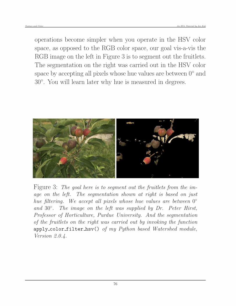
Texture and Color An RVL Tutorial by Avi Kak
operations become simpler when you operate in the HSV color
space, as opposed to the RGB color space, our goal vis-a-vis the
RGB image on the left in Figure 3 is to segment out the fruitlets.
The segmentation on the right was carried out in the HSV color
space by accepting all pixels whose hue values are between 0◦ and30◦. You will learn later why hue is measured in degrees.
Figure 3: The goal here is to segment out the fruitlets from the im-age on the left. The segmentation shown at right is based on just
hue filtering. We accept all pixels whose hue values are between 0◦
and 30◦. The image on the left was supplied by Dr. Peter Hirst,
Professor of Horticulture, Purdue University. And the segmentationof the fruitlets on the right was carried out by invoking the functionapply color filter hsv() of my Python based Watershed module,
Version 2.0.4.
76
Texture and Color An RVL Tutorial by Avi Kak
6.1: What Makes Learning About Color SoFrustrating
• Human perception of color is so complex and so nonlinear that it
cannot be described fully by any single computational model —
certainly not by any single linear model.
• Considering the nonlinearities involved, it is indeed amazing how
much mileage we have gotten out of the RGB and the closely
related HSI, HSV, HSL, etc., models. All these models can be
thought of as linear approximations to a nonlinear phenomenon. [For
an example of the nonlinearity of our color vision: When you darken the color orange, you get the color brown.
However, when you darken the color blue, it remains blue.] Attempts at coping with
the nonlinear aspects of color vision have resulted in color spaces
such as L*a*b*. These color spaces are based on the Opponent
Color Modeling of our color vision. On the other hand, RGB,
HSI/V/L, etc., are based on the Trichromatic Model of our color
vision.
• In addition to having to deal with the above mentioned modeling
complexities, what makes learning about color so frustrating for
an engineer are the nature of approximations that go into the
computational models. Here is a case in point: You will see
77

Texture and Color An RVL Tutorial by Avi Kak
frequent references to the RGB cube for the representation of
color. This representation obviously implies that the R, G, and
B components of color are orthogonal in some sense. But are
they really orthogonal in any sense at all?
• As it turns out, we assume the RGB cube to be orthogonal be-
cause that makes it easier to derive formulas for transformation
between different types of color spaces. This assumption also
makes it easier to visualize the three primary color components
(R, G, and B) when talking about colors. However, as you will
see later on in this tutorial, in a more “absolute” representation
of color — known as the X,Y,Z space — the RGB representation
is definitely non-orthogonal.
• Once you realize that the orthogonality of the RGB cube is really
just for convenience, you are left to wonder how much trust you
should place in the color-space transformation formulas that are
based on tilting the cube in a vector space and then deriving
equations for hue, saturation, and intensity from the tilted cube.
[You even wonder as to why you should believe that the colors on the surface of the tilted cube are the purest
(meaning the most saturated) hues.]
• If you are an engineer trying to understand color, another chal-
lenge you face is wrapping your head around what are known as
spectral colors. These are colors that would be produced by, say,
a tunable laser. You quickly find out that spectral colors are just
a very small subset of all the colors that humans are capable of
78

Texture and Color An RVL Tutorial by Avi Kak
experiencing. In general, the hue attribute of the human expe-
rience of color is based as much on the shape of the spectrum
of wavelengths in the light incident on the eye as it does on the
individual frequencies, but you never get a good sense of precise
nature of this dependence. [If we optically combine the light emitted from a pure red
laser with the light emitted from a pure blue laser, a human observer would perceive this combined light as
magenta. On the other hand, if we could produce a spectrally pure light at a wavelength halfway between blue
and red, that light would not be perceived as magenta. In other words, both the average wavelength and the
shape of the spectral distribution are important for characterizing hue.]
• Another source of frustration in learning about color is the im-
portance of ratios in almost every aspect of color. It is generally
believed that the sensation of color that we experience is deter-
mined primarily by the proportion of each of the three primary
colors in the light incident on the eye. [These would generally be the officially
formulated X, Y, and Z components that are deemed to be abstract. These could also be the R, G, and B
components] As you will see later in this tutorial, this implies that the
experience of color is described mostly by the points on a single
plane inside an XYZ or the RGB cube. Presumably, the colors
on this plane are the different possible hues. But it is not clear
as to what extent folks such as artists would agree with that. [On
account of its importance, this plane is called the Chromaticity Plane. Since all points on a plane possess only
two degrees of freedom, everything conveyed by the chromaticity plane can also be conveyed by its projection
on either the XY, or the YZ, or the XZ plane. Such a projection is referred to as the Chromatic Diagram.]
• Last but not the least is the great difficulty of making reliable
measurements of color if the goal is for these measurements to
79

Texture and Color An RVL Tutorial by Avi Kak
reflect the “true” colors of the object surfaces in a scene.
• The color that is captured by a camera depends significantly on
three factors: (1) the spectral composition of the illumination;
and (2) the light reflection properties of the object surfaces (some
surfaces are more specularly reflecting and others more diffuse);
and (3) the “true” color of the object surface (which depends on
what portion of the light spectrum is absorbed by the surface). If
you are looking at a scene that you are very familiar with, your
brain will do a great job of compensating for the confounding
effects of these three effects. However, a computer vision
algorithm must deal with all of the complexities cre-
ated by these effects. The guidance that the literature offers
on how to address these effects is entirely much too ad hoc.
• Finally, here are some additional sources of frustration when
wrapping your head around the literature on color: The words
“color” and “hue” are often used interchangeably, especially in ex-
planations of what is depicted by Chromaticity Planes and Chro-
maticity Diagrams. Whereas the word “chroma” in the context
of HSV and HSL spaces stands for basically the same thing as
saturation, the closely related word “chromaticity” is more about
depicting hues than saturation.
• As to why some of the issues I have mentioned above are frus-
trating will become clearer in the sections that follow. Note that
the color related discussion in the rest of this tutorial draws sig-
80

Texture and Color An RVL Tutorial by Avi Kak
nificantly from the following sources:
1. Margaretha Schwarz, Lynne Grewe, and Avi Kak, “Represen-
tation of Color and Segmentation of Color Images,” Purdue
University Technical Report, 1-1-1994. Paper 171, January
1994.
http://docs.lib.purdue.edu/ecetr/171
2. Lynne Grewe and A. C. Kak, “ Interactive Learning of a Multi-
Attribute Hash Table Classifier for Fast Object Recognition,”
Computer Vision and Image Understanding, pp. 387-416,
Vol. 61, No. 3, 1995.
3. Jae Byung Park and Avinash C. Kak, “A New Color Rep-
resentation for Non-White Illumination Conditions,” Purdue
University Technical Report, 6-1-2005, Paper 8, June 2005.
http://docs.lib.purdue.edu/ecetr/8
81

Texture and Color An RVL Tutorial by Avi Kak
6.2: Our Trichromatic Vision and the RGBModel of Color
• Although hue, saturation, and brightness describe naturally the
different aspects of color sensation experienced by humans, they
are not always useful for designing engineering systems.
• From an engineering perspective, a more useful description of
color is inspired by the fact that the retina of the human eye
contains three different types of photo receptors, with each type
possessing a different spectral sensitivity pattern. [These photo recep-
tors are commonly called cone cells.] By spectral sensitivity pattern I mean
the response of a photo receptor to incoming monochromatic light
at different wavelengths. The fact that the eye contains three dif-
ferent types of cone cells is referred to as the trichromaticity
property of the human visual system.
• The three spectral patterns — designated S, M, and L, which
stand for “Short”, “Medium”, and “Long” wavelengths — for
the three types of photo receptors are shown in Figure 4. [As
you can tell from the figure, these three spectral responses do not correspond to any
particular colors as we experience them. The L photo receptors are just as sensitive to
monochromatic green as to monochromatic yellow. The M photo receptors are primarily
82

Texture and Color An RVL Tutorial by Avi Kak
sensitive to green, but their sensitivity to red is not insignificant. The S photo receptors
are sensitive mostly to monochromatic blue. In the past, L, M, and S photo receptors
have been loosely associated with R (for red), G (for green), and B (for blue).] The
three spectral responses shown in the figure have commonly been
denoted hR(λ), hG(λ), and hB(λ) in the literature.
Figure 4: The retina of the human eye contains three different types
of photo receptors for color vision. The spectral responses of the threetypes are shown here. This figure is from the Wikipedia page on “Color
Vision”.
• Now assume for a moment that our goal is to design a vision
sensor that would help a backend processor perceive colors the
way the humans do. Ignoring for a moment what happens at
the higher levels in the brain, the trichromaticity of our visual
system would imply that if we could embed in the sensor three
83

Texture and Color An RVL Tutorial by Avi Kak
optical filters whose spectral properties are the same as hR(λ),
hG(λ), and hB(λ), all that the sensor would need to do would
be to generate the following three numbers at each pixel (since,
presumably, that is what the cone cells in the retina do):
R =∫
fill(λ)fref(λ)hR(λ)dλ
G =∫
fill(λ)fref(λ)hG(λ)dλ
B =∫
fill(λ)fref(λ)hB(λ)dλ (27)
where fill(λ) is the spectral composition of the illumination and
fref(λ) the spectral definition of the surface reflectivity in the
direction of the camera.
• Unfortunately, this logic for mimicking the human visual system
is not practical since it is not possible to create optical filters with
exactly the same spectral responses as for the three types of cone
cells in the retina. [And, even if we could, there would remain the issue of mimicking what
the human brain does with the RGB values thus generated — since the higher level processing of color
in the visual cortex of the brain remains largely a mystery.]
• Since it is not practical to design optical filters with the kinds of
responses shown in Fig. 4, approximations are necessary. The
common approximation consists of using filters with “single line”
responses for the three filters. [That typically means the R filter passes through
light at or in close vicinity to the 700 nm wavelength, the wavelength of the pure red hue. Similarly,
84
Texture and Color An RVL Tutorial by Avi Kak
the G filter passes through light at or in close vicinity to the 545 nm wavelength, the wavelength of the
pure green hue. And, the B filter passes through light at or in close vicinity to the 480 nm wavelength,
the wavelength of the pure blue hue.] Mathematically, this commonly used
engineering approximation is tantamount to saying that the filter
functions hR(λ), hG(λ) and hB(λ) in Eq. (27) are replaced by
the Dirac Delta functions δ(λ− λR), δ(λ− λG), and δ(λ− λB),
respectively.
• The primary justification for the above mentioned approximation
— the approximation of using “single-line” filters as opposed to
the filters whose spectral responses would be akin to those of the
cone cells in our retina — goes like this: Say we use a vision sensor
based on the above approximation to represent a given color by
three numbers R, G, and B. Now suppose we mix three spectrally
pure light beams, one red, one green, and one blue, in the same
proportion as the numbers R, G, and B. If a human observer
sees this composite beam, the color experienced by the human
would be roughly the same as the color in the original light beam
on the vision sensor. The words most open to questioning in
this justification are proportion and roughly; the former implies
using only two degree of freedom in the synthesis of the composite
beam and the latter is open to any interpretation.
• As it turns out, a number of spectrally pure colors corresponding
to different wavelengths cannot be synthesized by mixing the pure
R, G, and B components. This fact is made evident by Fig. 5
where it is shown how much red, how much green, and how much
85

Texture and Color An RVL Tutorial by Avi Kak
blue must be mixed in order to generate a spectrally pure color
at a given wavelength. The significance to be associated with
the wavelength band where the r(λ) function becomes negative
is most interesting: No spectrally pure color in this band can
be produced by any combination of red, green, and blue. The
negative values for r(λ) mean that if we were to combine the red
hue in proportion equal to the negative value of r(λ) to the green
and the blue hues in proportion to the positive values of g(λ)
and b(λ), respectively, we would obtain a color that, as seen by
the eye, would be the same as the spectrally pure color at that
wavelength. This would obviously be impossible since you cannot
have a negative proportion of a color component.
Figure 5: This figure shows how much red, how much green, and howmuch blue is needed at each wavelength to match the spectral color
at that wavelength. Obviously, the wavelengths where the curve goesnegative means that it is not possible to match those spectral colors
with a combination of R, G, and B. This figure is from the Wikipediapage on “CIE 1931 color space”.
86

Texture and Color An RVL Tutorial by Avi Kak
• Spectrally pure colors, although they represent only a fraction of
all possible colors, are obviously of engineering significance since
they can be generated with relative ease in a laboratory for mea-
surement and standardization. Since, as explained in the previous
bullet, it is not possible to generate even all the spectrally pure
colors by mixing red, green, and blue, these three colors can re-
ally not be thought of as being true primary colors. [We refer to
a set of three colors as the true primary colors if all other colors that are normally seen
by humans can be synthesized by mixing them.]
• It is the above stated inability to generate even the spectral colors
from R, G, and B that has led to the designation of three “ab-
stract” colors, denoted X , Y , and Z, as the primary colors. All
spectral colors in the visible band can be generated by a mixture
of the XYZ primaries. To repeat for emphasis, only the spectrally
pure colors can be generated by combining the X, Y, Z primary
colors. It may not be possible to generate a non-spectral color,
such as magenta, by combining the X, Y, Z primaries.
87

Texture and Color An RVL Tutorial by Avi Kak
6.3: Color Spaces
• So far I have mentioned three different types of color spaces:
RGB, HSI/V/L, and XYZ. Each of these color spaces amounts
to representing color by a point in three dimensions.
• A color space may also be two dimensional, which may come as a
surprise since color is inherently three dimensional. A prime ex-
ample of a 2D representation of color is the Chromaticity Space.
2D representations of color, as in a Chromaticity Space, are in-
tended to show only the range of hues that can be generated by
a given trio of primary colors.
• In the rest of this section, I’ll first explain the idea of the Chro-
maticity Space. Subsequently, I’ll discuss the relationship be-
tween different types of 3D color spaces.
The Chromaticity Space:
• As I mentioned previously, the XYZ space does a good job of rep-
resenting spectrally pure colors. In the XYZ space, an arbitrary
spectral color C may be represented as
88

Texture and Color An RVL Tutorial by Avi Kak
C = X ~X + Y ~Y + Z ~Z (28)
where X , Y , Z are the components of the color along the three
primaries that are symbolically represented by ~X , ~Y and ~Z.
• If the spectral distribution P (λ) of a color C is known, the com-
ponents X , Y , and Z may be found from
X = k∫
P (λ)x(λ)dλ
Y = k∫
P (λ)y(λ)dλ
Z = k∫
P (λ)z(λ)dλ (29)
where x(λ), y(λ), and z(λ) are functions of the wavelength as
shown in Fig. 6, and k is a value that depends on the device.
For example, a self-luminous object like a CRT has a k = 680
lumen/watt. Using vector notion, we may therefore say
C =
X
YZ
(30)
• I’ll now introduce the notion of the Chromaticity Space. Repre-
sentation of color in chromaticity space is based on an empirically
89

Texture and Color An RVL Tutorial by Avi Kak
Figure 6: This figure shows how much of each of the primaries X,Y, and Z it takes to produce a spectral color. This figure is from the
Wikipedia page on “CIE 1931 color space”.
verifiable premise that a large number of colors can be produced
by mixing the X, Y, and Z in just the right proportions, with-
out regard to their absolute values. To make this notion more
precise, consider the following normalized versions of X , Y , and
Z values in the XYZ space:
x =X
X + Y + Z
y =Y
X + Y + Z
z =Z
X + Y + Z(31)
• With the normalization shown above, the lowercase x, y, and z
will always obey the following constraint:
90

Texture and Color An RVL Tutorial by Avi Kak
x+ y + z = 1 (32)
• What is of engineering significance here is that as long as X , Y
and Z are in the same ratio vis-a-vis one another, the values of x,
y and z will remain unchanged and the constraint shown above
will be satisfied.
• To give the reader a greater insight into the transformation from
XYZ to xyz, consider the following two dimensional case:
u′ =u
u+ v
v′ =v
u+ v(33)
Just by substitution, the reader can easily verify that for all the
points along the line OA in the (u, v) space in Fig. 7, the corre-
sponding u′ and v′ values will be at A′. Similarly, all the points
on the line OB will be mapped to the point B′, and so on. [In other
words, the entire positive quadrant in the (u, v) plane will be mapped to the line PQ. Mathematically,
this fact is inferred readily from the observation that u′ + v′ must equal 1 for all mapped points.]
• Extending our two dimensional example to the three dimensional
case of XYZ (Fig. 8a), we see that for all the values of X, Y, and
Z, the value of x, y, and z will be confined to the planar surface
91

Texture and Color An RVL Tutorial by Avi Kak
Figure 7: This figure shows how a normalization of the coordinatesin a 2D plane can map all the first quadrant points to the line PQ.
denoted by P, Q and S in Fig. 8a. This plane is referred to as
the Chromaticity Plane. The projection of this planar surface
on one of the orthogonal planes constitutes the Chromaticity
Diagram. Usually, the projection on the XY plane is taken.
• Remember the main justification for using x, y and z is that a
large majority of at least the pure spectral colors can be produced
simply by maintaining the right proportionalities between the
three constituents X, Y, and Z. Translating into our diagram of
Fig. 8, that means that each point on the the planar surface
bounded by P, Q, and S corresponds to some color. The colors
at the different points of this plane are shown in Fig. 9 in the
form of a Chromaticity Plane.
• When these color on a Chromaticity Plane are projected on to
92
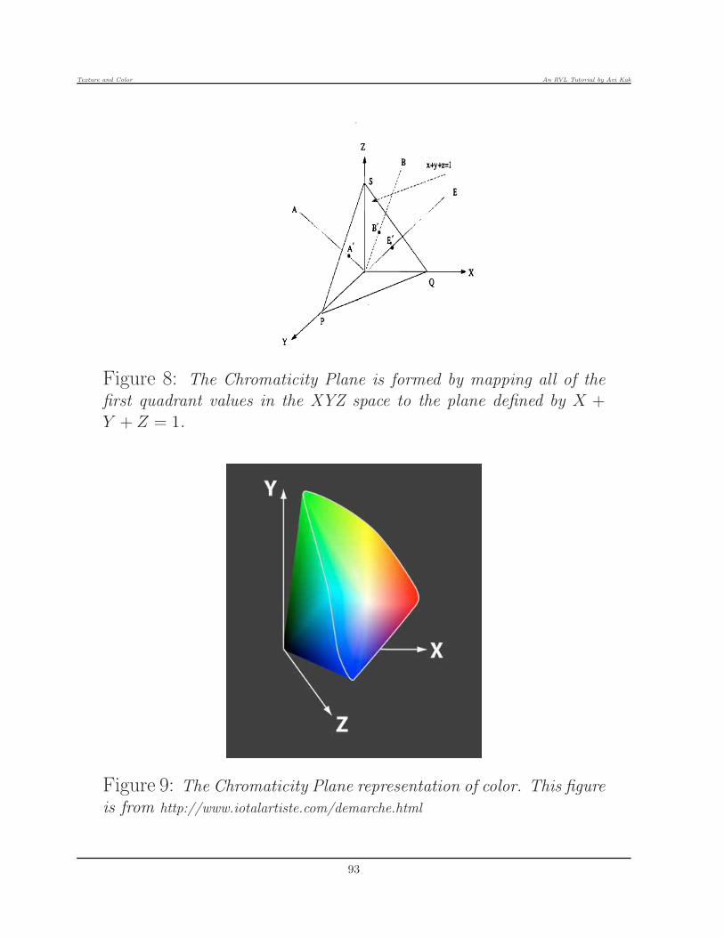
Texture and Color An RVL Tutorial by Avi Kak
Figure 8: The Chromaticity Plane is formed by mapping all of thefirst quadrant values in the XYZ space to the plane defined by X +
Y + Z = 1.
Figure 9: The Chromaticity Plane representation of color. This figureis from http://www.iotalartiste.com/demarche.html
93

Texture and Color An RVL Tutorial by Avi Kak
the XY plane, we get the corresponding Chromaticity Diagram,
as shown in Fig. 10. This figure points to the main use of the
color depiction through Chromaticity Planes or Diagrams. The
triangle that is shown inside the overall rounded cone corresponds
to the sRGB color space. [sRGB is the RGB color space as standardized by CEI.
The prefix letter “s” stands for “standardized”.] The colors that are outside the
sRGB gamut, while discernible to humans, cannot be reproduced
by typical electronic displays. [By gamut, we mean the colors that can be created
through a linear mixture of R, G, and B.] The colors at the periphery of the large
rounded cone are the pure spectral colors. So if you could tune
the wavelength of a laser, you would move around the rounded
perimeter shown in the diagram.
• The boundary colors in the chromaticity depictions of the sort in
Figs. 9 and 10 correspond to those colors that can be produced
by spectrally pure light. For example, if we were to take a tunable
laser and change its wavelength continuously from one end of the
visible spectrum to the other, as shown in Fig. 10 we would obtain
colors corresponding to a clockwise traversal of the boundary
of the large rounded cone. So, the interior colors of this cone
correspond to those that would require combining laser beams of
different colors.
• Figure 11 again shows the Chromaticity Plane conceptually in the
positive quadrant of the XYZ space. Note that this time we have
roughly marked the points on the plane that would correspond
94

Texture and Color An RVL Tutorial by Avi Kak
Figure 10: Projection of the Chromaticity Plane on the XY-plane
gives us the Chromaticity Diagram. The triangle in the middle is thesRGB color gamut that most electronic displays are capable of dis-
playing. The larger rounded cone is what the human eye can see. Thecolors on the periphery of the large rounded cone are the spectral col-
ors. As you change the wavelength of a monochromatic light beam overthe entire spectral range visible to humans, you will move along the
rounded perimeter shown in the diagram. The arc in the middle showswhat is known as the Planckian Locus. The numbers shown along thearc are the temperatures to which you must raise an incandescent black
body for it to emit the light at that point in the diagram.
95
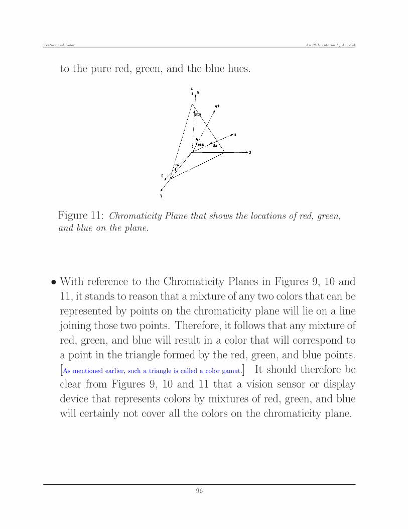
Texture and Color An RVL Tutorial by Avi Kak
to the pure red, green, and the blue hues.
Figure 11: Chromaticity Plane that shows the locations of red, green,and blue on the plane.
• With reference to the Chromaticity Planes in Figures 9, 10 and
11, it stands to reason that a mixture of any two colors that can be
represented by points on the chromaticity plane will lie on a line
joining those two points. Therefore, it follows that any mixture of
red, green, and blue will result in a color that will correspond to
a point in the triangle formed by the red, green, and blue points.
[As mentioned earlier, such a triangle is called a color gamut.] It should therefore be
clear from Figures 9, 10 and 11 that a vision sensor or display
device that represents colors by mixtures of red, green, and blue
will certainly not cover all the colors on the chromaticity plane.
96

Texture and Color An RVL Tutorial by Avi Kak
RGB Space:
• Commonly used hardware devices for capturing and displaying
color images use the RGB representation, meaning that each color
is expressed by a mixture of red, green, and blue.
• Strictly speaking, as made clear by Figures 10 and 11, the positive
“quadrant” of the RGB space is a subset of the positive quadrant
the XYZ space. This fact is made clear by Fig. 11 where we have
drawn the X, Y, and Z vectors in an orthogonal frame and the
vectors corresponding to R, G, and B are then shown by drawing
lines through the corresponding points on the chromaticity plane.
[Theoretically speaking, the three RGB vectors span the same space as the XYZ vectors. However,
since colors can only be made from positive mixtures, the positive “quadrant” of the RGB space is a
subset of the positive quadrant of the XYZ space.]
• The R, G, and B components of color are typically expressed as
8-bit integers. That is, the value of each color component is an
integer in the range [0, 255].
• Fig. 12 shows the colors on the surface of the RGB cube as the
cube is viewed inwards from the positive quadrant. [It may seem
like a contradiction that while the colors white, red, green, and blue are coplanar in
Fig. 11, they are non-coplanar in the RGB cube of Fig. 12. This contradiction is not
real for the following reason: In the chromaticity depiction, every color is forced to lie
on the chromaticity plane of Fig. 11 whether or not it really does. In other words,
97
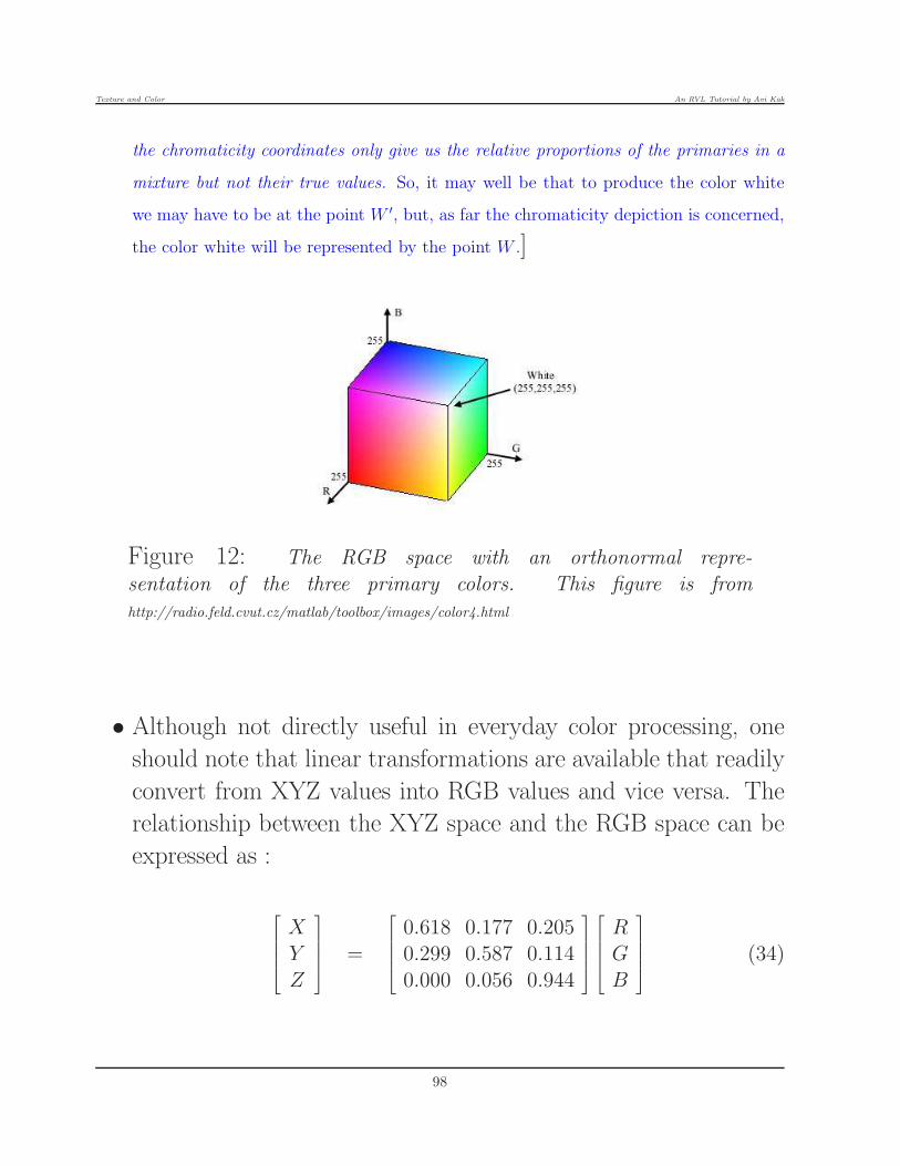
Texture and Color An RVL Tutorial by Avi Kak
the chromaticity coordinates only give us the relative proportions of the primaries in a
mixture but not their true values. So, it may well be that to produce the color white
we may have to be at the point W ′, but, as far the chromaticity depiction is concerned,
the color white will be represented by the point W .]
Figure 12: The RGB space with an orthonormal repre-
sentation of the three primary colors. This figure is fromhttp://radio.feld.cvut.cz/matlab/toolbox/images/color4.html
• Although not directly useful in everyday color processing, one
should note that linear transformations are available that readily
convert from XYZ values into RGB values and vice versa. The
relationship between the XYZ space and the RGB space can be
expressed as :
XY
Z
=
0.618 0.177 0.2050.299 0.587 0.114
0.000 0.056 0.944
RG
B
(34)
98

Texture and Color An RVL Tutorial by Avi Kak
• The reader might wonder that if a linear transformation can con-
vert any XYZ value into a corresponding RGB value, and if it
is possible to generate all pure spectral colors by mixing XYZ
primaries, why it is not possible to generate all such colors with
mixtures of R, G, and B. The answer is that there is no guar-
antee that such transformations would yield positive weights for
the RGB colors.
HSI Space:
• We have already mentioned the HSI (Hue, Saturation, Intensity)
scheme for representing colors. The HSI coordinates are cylindri-
cal, with H being represented by the azimuthal angle measured
around the vertical axis, S by the outward radial distance, and
I the height along the vertical (Fig. 13).
• As you would expect, [0.0, 360.0] in degrees is the value range for
H. And the value range is [0.0, 1.0] for both S and I .
• The red hue is placed at H = 0◦, the green at H = 120◦, andthe blue at H = 240◦. The point I = 1 on the vertical axis
corresponds to pure white, and the origin to the black color since
the intensity will be zero there.
99

Texture and Color An RVL Tutorial by Avi Kak
θ for hue
0 degreeRed Hue
120 degreesGreen Hue
240 degrees
saturation
Intensity
White, I=1.0
BlackI=0.0
Blue Hue
Figure 13: The HSI space
100

Texture and Color An RVL Tutorial by Avi Kak
• Since the HSI coordinates are more intuitive to humans and since
RGB is what is used by most digital devices for image capture
and display, it is important to establish a transformation between
the two spaces.
• To set up a transformation between RGB and HSI, we line up
the diagonal of the the RGB cube in Fig. 12 with the vertical
axis of Fig. 13. We obviously want the (255, 255, 255) point of
the RGB cube to become coincident with the I = 1 point on the
vertical axis of the HSI cylindrical representation since these two
points in their respective spaces represent the color white (Fig.
14). [IMPORTANT: When aligning the RGB cube with the HSI coodinates, the R, G, and B
values are mapped to the [0, 1] interval from their original [0, 255 value range.]
• In Fig. 14, the rotational orientation of the RGB cube is such that
the red axis of the cube is in same azimuthal plane (the H = O◦
plane) that contains the red hue in HSI. This will automatically
cause the green axis of the RGB cube to fall on the azimuthal
plane corresponding to H = 120◦. Recall that the point at H =
120◦, S = 1, and I = 1 designates green in the HSI system.
Similarly, for the blue axis of the RGB frame.
• One may now write down the transformation equations that take
a color point from RGB to HSI and vice versa. To facilitate
the derivation of these equations, let’s momentarily assume that
the HSI system is embedded in a Cartesian frame whose axes
101

Texture and Color An RVL Tutorial by Avi Kak
u
v
w
G
R
B
C
HS
I
Cu
Cv
Cw
Figure 14: The RGB cube is tilted and rotated in the manner shown
here for deriving a relationship between RGB and HSI coordinates.The longest diagonal of the cube becomes aligned with the vertical In-
tensity (I) axis in HSI. The Hue (H) coordinates of HSI is measuredcounterclockwise from the projection of the RGB cube’s red corner onthe horizontal plane. Saturation (S) is the radial distance from the
vertical axis.
102

Texture and Color An RVL Tutorial by Avi Kak
are labeled U, V and W, as shown in Fig. 14. Consider now
an arbitrary color point C, whose projections on the U , V , W
axes are given by Cu, Cv, and Cw. Clearly, then the HSI values
associated with this color point are given by
H = tan−1 Cv
Cu
S =√
C2u + C2
v
I = Cw (35)
• To express the transformation from RGB to HSI, all we now
need do is express an arbitrary point C in the RGB points in the
UVW frame. Let the coordinates of this point in the RGB frame
be given by R, G, and B and the corresponding coordinates in
the UVW frame by Cu, Cv, and Cw. [IMPORTANT: In the formulas here,
we assume that the value of R, G, and B are normalized to the [0, 1] range.] Then,
Cu =
√
√
√
√
2R−G−B
6
Cv =
√
√
√
√
G−B
2
Cw =R +G+ B
3(36)
103

Texture and Color An RVL Tutorial by Avi Kak
• Since the arctan in Eq. (35) for H is a multivalued function, the
value of H needs to be specified more precisely. Ambiguities are
resolved by using the following set of formulas for H:
H = cos−1
Cu√
C2u + C2
v
if G >= B
= 360 − cos−1
Cu√
C2u + C2
v
if G < B
(37)
• Since there is no guarantee that the computed value for S will
not exceed 1, it is normalized as follows:
S =S
Smax
(38)
which results in the following equation for S :
S = 1 − 3 ·min(R,G,B)
R +G+B(39)
Although useful in an approximate sense, there are serious con-
ceptual shortcomings in the above derivation of the transforma-
tion. First and foremost, we assumed the RGB space to be or-
thogonal. As mentioned earlier, while the R, G, and B vectors
may be linearly independent in the XYZ space, they are certainly
not orthogonal. Their orthogonality in Fig. 12 was meant simply
to make easier the visualization of color distributions.
104
Texture and Color An RVL Tutorial by Avi Kak
• So, strictly speaking, to derive a transformation between the RGB
space and HSI space, one must derive transformation equations
that relate the RGB vectors, as shown in Fig. 11, with the HSI
space as shown in Fig. 13, the transformation being controlled
on the one hand by the alignment of the white points in the two
spaces and, on the other, by the requirements that the R, G, and
B vectors in Fig. 11 pass through the the designated points for the
three colors in the HSI cylinder in Fig. 13. Such a transformation
would be very complex for obvious reasons. However, it is possible
to make reasonable approximations.
• The goal of what I have described so far was to give the reader a
sense how one can set up a connection between the RGB and the
HSI color spaces. Using this reasoning, along with some refine-
ments related to explicitly factoring in the piecewise continuous
nature of the boundary of the RGB cube, I’ll show below the
transformation equations that have actually been implemented
in several software libraries: [These and other transformations like the one shown
below are taken from http://dystopiancode.blogspot.comwith some modifications by me to reflect
how they are actually implemented in code.]
• In the RGB to HSI transformation shown below, the input con-
sists of a triplet of values (R,G,B), with each color component
expressed as a floating point number in the [0, 1] range. And the
output of the transformation is a triplet of values (H,S, I), with
H expressed in degrees.
105

Texture and Color An RVL Tutorial by Avi Kak
M = max(R,G,B)
m = min(R,G,B)
c = M −m
I =R +G+B
3
H =
60(
G−B
cmod 6
)
if M = R, c 6= 0
60(
B−R
c+ 2
)
if M = G, c 6= 0
60(
R−G
c+ 4
)
if M = B, c 6= 0
0.0 if C = 0
S =
[
0 if c = 01− m
lif c 6= 0
(40)
• Note that when the three color components, R, G, and B are
equal, you are supposed to get a pure gray point on the vertical
axis of the HSI coordinate system. That’s what the formulas
shown above do. In such cases, c is zero. That causes H to be
set to 0, S to also be set to 0, and I to be set to one of the R, G,
B values (since they will all be the same). Yes, the point H = 0◦
means pure red. However, that is not an issue since it is at a
radial distance of 0 from the vertical axis. Also note that using
the condition c 6= 0 in the formulas for H protects us against
division by 0 when all three color components are the same.
• Shown below are the formulas that take you from HSI to RGB.
In these formulas, we represent a point in the HSI space by the
triplet (H,S, I). The variable hr stands for the value of H in
radians (as opposed to degrees) and the variable hk is the cor-
responding angle offset in each of the 120◦ segments of the hue
106

Texture and Color An RVL Tutorial by Avi Kak
circle. As you know from the previous discussion, the 0◦ point forH corresponds to pure red, the 120◦ point to pure green, and the
240◦ point to pure blue. In terms of radians these points are at
0, 2π/3 and 4π/3 radians. [Strictly speaking, I should not have shown the expression
for calculating the three variables (x, y, z) in a single line — since the calculation for z requires that
you first have calculated the values for x and y.] The input to the transforma-
tion shown below consists of a triplet of values (H,S, I), with H
expressed in degrees. And the output of the transformation con-
sists of a triplet of values (R,G,B) with each color component
expressed as a floating point value in the [0, 1] range.
hr = 0.0174532925×H
hk =
hr if 0 ≤ hr ≤ 2
3π
hr − 2
3π if 2
3π < hr ≤ 4
3π
hr − 4
3π if 4
3π < hr < 2π
(x, y, z) =
(
1− S
3,
1 + S cos(hk)
3 cos(π3− hk)
, 1− (x+ y)
)
(x′, y′, z′) =(
3× I × x, 3× I × y, 3× I × z)
(R,G,B) =
(I, I, I) if S = 0(y′, z′, x′) if 0 ≤ hr ≤ 2
3π
(x′, y′, z′) if 2
3π < hr ≤ 4
3π
(z′, y′, x′) if 4
3π < hr < 2π
(41)
HSV And HSL Spaces:
• The HSI representation of color tends to underestimate the in-
tensity values at the pixels. In the HSI model, the intensity at
a pixel is supposed to capture the “energy” of the light your
107
Texture and Color An RVL Tutorial by Avi Kak
eye wants to associate with that pixel. However, when you set
I = (R+G+B)/3, you are basically setting I to the average of
the “energies” that you may associate separately with the three
color channels. If you really think about it, that does not seem
like the correct thing to do. [Let’s say that an image display looks very bright — meaning
that its pixels pack much light “energy” —because of the bright reds in the image. And let’s also assume that
there is no blue or green in the image. By setting I = R/3 in this case, the HSI formula would discount the
“energy” coming off the pixels by two-thirds — which really does not make a whole lot of sense. The fact that
HSI mutes the I values unless it sees strength in all three color channels can be highly problematic for
computer vision algorithms. For extracting the shape information, many computer vision algorithms
depend primarily on the intensity attributes at the pixels.]
• This shortcoming of HSI is remedied in the HSV and HSL models
of color vision. So as not to cause any confusion between different
ways of calculating the intensities, what is I in HSI is represented
by V for “Value” in HSV, and by L for “Lightness” in HSL.
Whereas the calculation of H remains the same in HSV and HSL
as as in HSI, the formulas for how V and L are calculated are very
different, as you would expect. The different ways of calculating
the intensity result in a small modification to the formulas for
calculating the saturation. [The value ranges for the three variables in both HSV and
HSL remain the same as for HSI. That is, H values span [0.0, 360.0], S values span [0.0, 1.0]; and both
V and L values span [0.0, 1.0].]
• The V in HSV is calculated asmax(R,G,B). And the L in HSL
is calculated as max(R,G,B)+min(R,G,B)2 .
108

Texture and Color An RVL Tutorial by Avi Kak
• The S in HSV is calculated as max(R,G,B)−min(R,G,B)V
. And the
same in HSL is calculated as max(R,G,B)−min(R,G,B)1−abs(2L−1) .
• Fig. 15 on the next page shows a rather dramatic comparison of
the intensity values calculated by the different color models.
• Since HSV tends to be employed more commonly compared to
HSL, I’ll show below how the transformation formulas as they
have actually been implemented in several software libraries for
going from RGB to HSV and back.
• Here are the formulas that take you from RGB to HSV. The input
to the transformation shown below consists of a triplet of values
(R,G,B) with the individual color components normalized to
the [0, 1] range.
M = max(R,G,B)
m = min(R,G,B)
c = M −m
V = M
H =
60(
G−B
cmod 6
)
if M = R, c 6= 0
60(
B−R
c+ 2
)
if M = G, c 6= 0
60(
R−G
c+ 4
)
if M = B, c 6= 0
0 if c = 0
S =c
V(42)
109
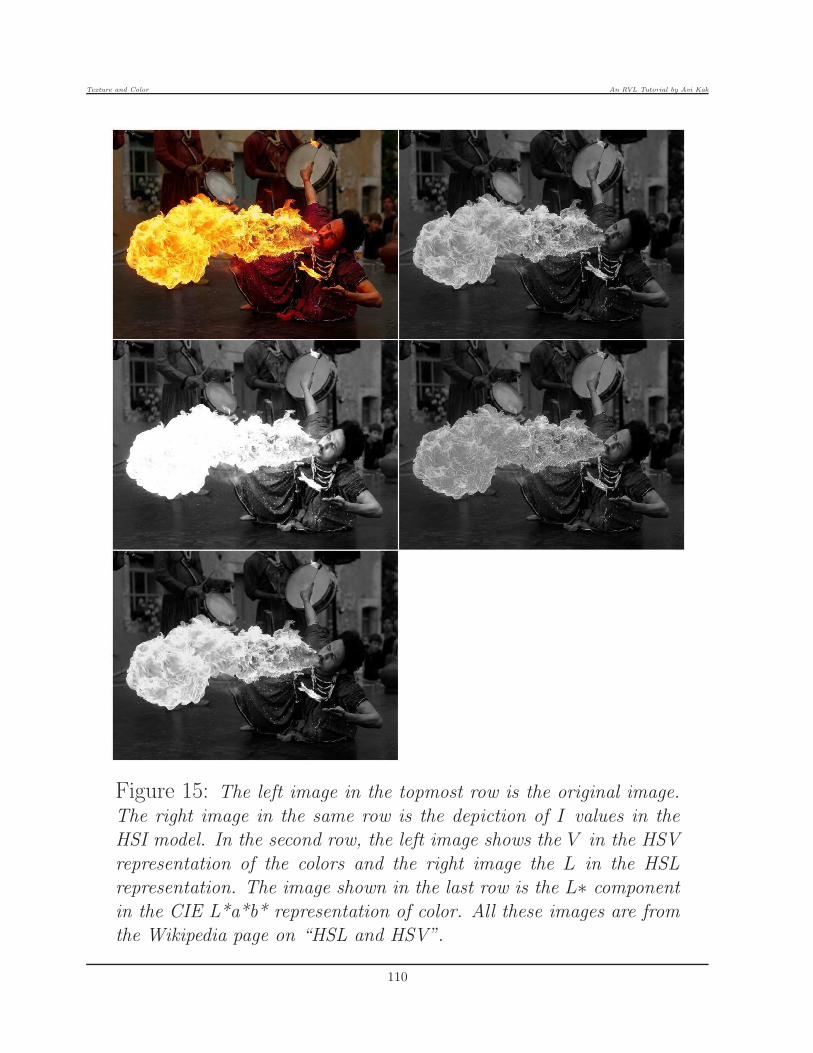
Texture and Color An RVL Tutorial by Avi Kak
Figure 15: The left image in the topmost row is the original image.
The right image in the same row is the depiction of I values in theHSI model. In the second row, the left image shows the V in the HSV
representation of the colors and the right image the L in the HSLrepresentation. The image shown in the last row is the L∗ component
in the CIE L*a*b* representation of color. All these images are fromthe Wikipedia page on “HSL and HSV”.
110

Texture and Color An RVL Tutorial by Avi Kak
• In the formulas shown above, note how we protect the calculation
of H against division by 0 when R, G, and B have exactly the
same values. We know that when you mix these primary colors in
equal amounts, you get pure gray, which is a point on the vertical
axis of the HSV coordinate frame. When c = 0, these formulas
return (M, 0, 0), which is a point on the vertical axis of the HSV
space.
• And, finally, shown are the corresponding formulas for going from
HSV to RGB. The input to the transformation shown below con-
sists of triplet of values (H,S, V ). Note that the returned values
for the individual colors in the triplet (R,G,B) are in the range
[0, 1].
c = V × S
m = V − c
x = c(
1−∣
∣
∣
H
60mod 2 − 1
∣
∣
∣
)
(R,G,B) =
(c+m, x+m,m) if 0 ≤ H ≤ 60(x+m, c+m,m) if 60 < H ≤ 120(m, c+m, x+m) if 120 < H ≤ 180(m, x+m, c+m) if 180 < H ≤ 240(x+m,m, c+m) if 240 < H ≤ 300(c+m,m, x+m) if 300 < H ≤ 360
(43)
Opponent Color Spaces
• It has been suggested by many researchers who work on the psy-
111
Texture and Color An RVL Tutorial by Avi Kak
chophysics of color vision that the human experience of color is
marked by what are referred to as the opponent colors. Oppo-
nent colors are based on the notion that the cells in the retina
collaborate to form receptor complexes and, through the receptor
complexes, the three independent components of color that the
eye can see are along the red-green, blue-yellow, and black-white
dimensions. [The “red-green”, “blue-yellow”, and “black-white” are referred to as opponent pairs.
You can think of red as opposed to green, blue as opposed to yellow, and black as opposed to white. The
human brain wants to receive a single signal for each of the three opposites.]
• That is, as shown in Figure 16, the visual cortex in the brain gets
three independent signals from the retina: one regarding how
much of the red-green dimension exists at a point in the scene; a
second regarding how much of the blue-yellow dimension exists;
and a third regarding how much of the black-white dimension
exists at a scene point. The receptor complexes that perceive
these three different dimensions of the color are referred to as the
opponent cells. [The fact that we can see orange, whose three independent components would be
red, yellow, and white, and the fact that we cannot see reddish-green or yellowish-blue supports the opponent
color model. Since the two color components in a reddish-green mixture are along the same dimension, the red-
green receptor complex is unable to discern them separately.] Note the very important fact
that if there was not considerable overlap between the spectral
sensitivities shown in Fig. 4 for L, M, and S, it would not be
possible for a receptor complex to see the colors in the opponent
manner.
• The L*a*b* is currently the most widely used opponent color
112
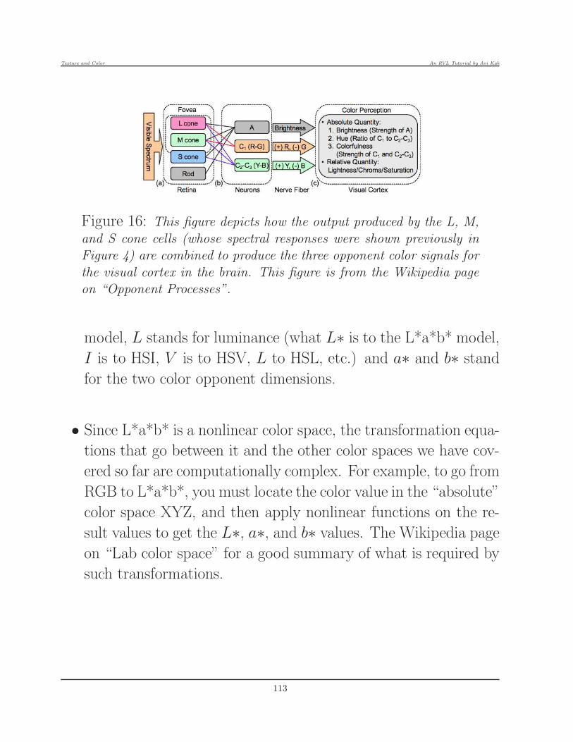
Texture and Color An RVL Tutorial by Avi Kak
Figure 16: This figure depicts how the output produced by the L, M,
and S cone cells (whose spectral responses were shown previously inFigure 4) are combined to produce the three opponent color signals for
the visual cortex in the brain. This figure is from the Wikipedia pageon “Opponent Processes”.
model, L stands for luminance (what L∗ is to the L*a*b* model,
I is to HSI, V is to HSV, L to HSL, etc.) and a∗ and b∗ stand
for the two color opponent dimensions.
• Since L*a*b* is a nonlinear color space, the transformation equa-
tions that go between it and the other color spaces we have cov-
ered so far are computationally complex. For example, to go from
RGB to L*a*b*, you must locate the color value in the “absolute”
color space XYZ, and then apply nonlinear functions on the re-
sult values to get the L∗, a∗, and b∗ values. The Wikipedia page
on “Lab color space” for a good summary of what is required by
such transformations.
113

Texture and Color An RVL Tutorial by Avi Kak
CMY Space:
• Understanding color in RGB space is important because digi-
tal cameras produce R, G, and B signals and because display
monitors take R, G, and B signals to output color images. Un-
derstanding color in HSI/HSV/HSL space is important because
it is in that space we as humans understand color the best.
• However, When it comes to making hardcopies of color images,
one must understand color in what is referred to as Cyan, Ma-
genta, Yellow space or the CMY space.
• Just as red, green, and blue are additive “primaries” (meaning
that we may attempt to express any emitted color as an additive
mixture of these three colors), cyan, magenta, and yellow are
subtractive primaries. To explain what that means, shown in
Fig. 17 on the next page is the color wheel for pigment
hues. [On a color wheel, the pigments corresponding to any two hues that are one hue apart may
be mixed to yield a pigment whose hue is in the middle. For example, if we mix together the cyan and
magenta pigments, we obtain the blue pigment.]
• When we say a pigment hue on the color wheel of Fig. 17 is
subtractive, what we mean is that if we shine white light on a
surface coated with that pigment, it will absorb from the white
light the hue at the opposite point on the color circle. Assume
114

Texture and Color An RVL Tutorial by Avi Kak
Figure 17: The color wheel for pigment hues. The colors thatare diametrically opposites are subtractive vis-a-vis each other. The
opposite color pairs are considered to be complementary. The twocolors that are immediately adjacent to each color are considered
to be analogous. Finally, the three colors at the vertices of anequilateral inside the wheel are considered to form a triad. Fromhttp://www.dimensionsthruart.com/
that a surface is coated with the cyan pigment. Now assume that
a beam of white light rich in all hues is incident on the surface,
as depicted in the figure. The pigment will absorb the red hue
and the distribution of hues in the reflected light will carry all
hues except red. Since the reflected light must again be thought
of as emitted light, we must add the hues on the color wheel to
determine the color of the reflected beam. The hues that are
opposite will add up to white. Therefore, the reflected light will
bear the color of cyan (since its opposite, red, would be absorbed
by the pigment), in addition to containing some white light. In
other words, the reflected light will be an unsaturated version of
cyan. [This explanation should also point to the fact that the colors seen in the white
light that is reflected off colored object surfaces can never appear to intense since much
115
Texture and Color An RVL Tutorial by Avi Kak
of the white light will remain in what is reflected. In other words, you have to use
emitted light for constructing brilliant displays — as you might have noticed from the
more billboards along highways these days.]
• Just as a video monitor has separate light emitters for red, green,
and blue, a hard copy printer has separate ”pens” for cyan, ma-
genta, and yellow. Suppose a pixel produced by a color camera
has the following components of R, G, and B: R = 0.8, G = 0.3,
and B = 0.4, where for the sake of the explanation here, we
have assumed the range [0.0, 1.0] for the three color components.
When this pixel is displayed on a color calibrated video moni-
tor, these RGB values will cause the monitor pixel to possess the
right color. However, when the same pixel is sent for display to
a hardcopy printer, the values sent to the cyan, magenta, and
yellow pens must be
C = 0.2 = 1− R
M = 0.7 = 1−G
Y = 0.6 = 1− B
(44)
• With the CMY values set as shown above, C being 0.2 will cause
the deposited cyan pigment to absorb 0.2 fraction of the red hue
in the supposedly white illumination of the hardcopy surface,
116

Texture and Color An RVL Tutorial by Avi Kak
releasing 0.8 of the red hue in the direction of the observer. Sim-
ilarly, with M and Y for the generation of the correct values of G
and B for an observer.
• This transformation between RGB and the CMY values required
to produce the correct RGB in light reflected from a hardcopy is
expressed succinctly by
CM
Y
=
11
1
−
RG
B
(45)
117

Texture and Color An RVL Tutorial by Avi Kak
6.4: The Great Difficulty of Measuring theTrue Color of an Object Surface
• From the standpoint of computer vision, our goal is obviously to
associate with each pixel in an image a color value that represents
the true color of the object surface that gave rise to the pixel.
• Unfortunately, what makes the measurement of that color com-
plicated are the following factors:
– The direction of illumination. When illumination is not purely dif-
fuse, the color of the light coming off an object surface depends onthe direction of the incident illumination. In general, now the lightcoming off the surface will have a specular component and a diffuse
component. The “true” color of a surface is normally associated withjust the diffuse light coming off the surface.
– The reflection properties of the object surface with regard to howmuch of the incident light is reflected specularly and how through
diffuse processes. This would depend on the roughness (texture) ofthe surface.
– The color of the illumination. The color of the light coming off asurface depends significantly on the color of the illumination.
– The intensity of the illumination. The dependence on the intensitymeans that, if you are recording an image of an outdoor scene during
118

Texture and Color An RVL Tutorial by Avi Kak
daytime, the color measurements for same surface will be differentdepending on whether it is directly in the sunlight or whether it is in
a shadow. [This is partly the same phenomenon as captured by thenonlinearities of the human color vision. See the earlier discussion on
the Opponent Color Spaces such as L*a*b* in the previous section.]
– Color filtering by the hardware. The spectral properties of the three
color filters used by the camera that are used to break incoming lightinto ostensibly the R, G, and B components.
• That the color of the light coming off an object surface depends signifi-cantly on the color composition of the illumination is illustrated by Fig.
18. As you can see in the figure, a yellow ball looks green under mostlyblue illumination. This figure also shows how one can algorithmically
correct for illumination induced distortion of the color of a surface. Theresult shown in (c) of the figure was obtained through the use of anillumination-adaptive color space that was introduced in 2005 by Park
and Kak in the report “A New Color Representation for Non-White Il-lumination Conditions,” that was cited at the end of Section 6.1.
• For another example of illumination dependency of the image
recorded by a digital camera, shown in the top row of Fig. 19
are four different images for the same plastic toy. These images
were recorded under the following illuminations: (1) florescent,
(2) blue incandescent, (3) green incandescent, and (4) tungston.
The second row demonstrates the extent to which the true color
of the toy was restored in each case by the illumination-adaptive
color representation of Park and Kak mentioned in the previous
bullet.
119

Texture and Color An RVL Tutorial by Avi Kak
Figure 18: (a) A green ball and a yellow ball imaged under ambientwhite-light illumination. (b) The yellow ball imaged under blue illu-
mination. It now looks quite a bit like the green ball. (c) The image of(b) after its processing by the algorithm in the 2005 Park and Kak re-port titled “A New Color Representation for Non-White Illumination
Conditions” that was cited at the end of Section 6.1.
• Regarding the dependence of the measured color on the measur-
ing device itself, note that the photoelectric cells in the camera
imaging sensor (which may either be a CCD sensor or a CMOS
sensor) use color filters centered around the R, G, and B wave-
lengths. So the 3-dimensional measurement of the color at each
pixel also depends on the spectral properties of these filters. [The
three measurements at each pixel may be recorded by a single sensor chip that contains a mosaic of cells in which
groupings of three adjacent cells are used for measuring the R, G, B components separately. An incoming light
ray is deflected to each of three cells in a grouping and light for each cell passed through a color-sensitive filter
specific to that cell. An alternative consists of using three separate sensor chips, one for each color component,
and a set of prisms that are shaped to deflect a particular color component to each chip.]
• Figure 20 points to the issues involved in the dependence of the
120

Texture and Color An RVL Tutorial by Avi Kak
Figure 19: The photos in the top row are of the same plastic toy
and were recorded by the same digital camera using four different il-lumination sources: (1) florescent, (2) blue incandescent, (3) green
incandescent, and (4) tungston. The second row demonstrates the ex-tent to which the true color of the toy was restored in each case by the
illumination-adaptive color representation method of Park and Kak.
121

Texture and Color An RVL Tutorial by Avi Kak
measured color on the direction of the illumination. The main
issue here is that the diffuse light that is reflected off a surface
(which is the light we want a camera to capture for characterizing
the color of the surface) has a cosine dependence on the angle of
illumination to the perpendicular to the surface. [For a given incident
light beam, we have shown reflected light as consisting of specular and diffuse components, the components
being additive. The specular and the diffuse components of the reflected light are also known as the surface
component and the body component, respectively. Light reflected by homogeneous materials such as metals
is dominated by the surface components, whereas the light reflected by inhomogeneous material is dominated
by the body component. ]
Figure 20: Si represents the specular reflection resulting from theillumination source i. The diffuse reflection from any illuminationsource radiates out in all directions. The radius of the arc labeled Di
represents the magnitude of the diffuse reflection from the illuminationsource i. Note that this magnitude depends on the cosine of the angle
the illumination source makes with the surface.
• The dependence of the reflected diffuse color light on the angle
122

Texture and Color An RVL Tutorial by Avi Kak
of illumination is illustrated with some actual measurements in
Fig. 22. The two results shown in that figure are for the pink
and the yellow objects in the pile shown in Figure 21. For the
two experimental results shown in Figure 22, the position/angle
of the source of illumination and the camera were kept fixed while
the surface was tilted in increments of 15◦.
Figure 21: The yellow and the white objects shown in this pile wereused for demonstrating the dependence of the measured color on theorientation of a surface.
• To fully appreciate the results shown in Fig. 22, note that at
the relatively small slant angle of 15◦, which is also the angle
of incidence, we would expect the specular component of the
reflected light to be the strongest, as can be seen in both the
results in the figure.
• When the camera is situated in a direction where the angle of
123
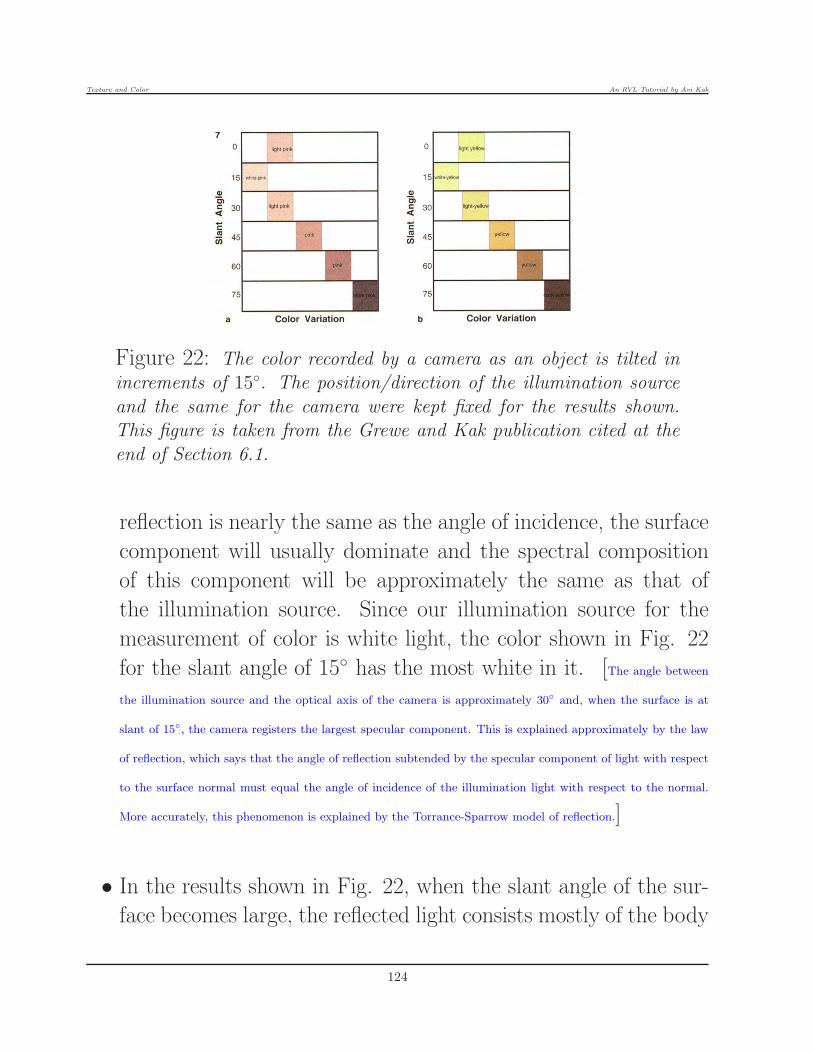
Texture and Color An RVL Tutorial by Avi Kak
Figure 22: The color recorded by a camera as an object is tilted inincrements of 15◦. The position/direction of the illumination source
and the same for the camera were kept fixed for the results shown.This figure is taken from the Grewe and Kak publication cited at the
end of Section 6.1.
reflection is nearly the same as the angle of incidence, the surface
component will usually dominate and the spectral composition
of this component will be approximately the same as that of
the illumination source. Since our illumination source for the
measurement of color is white light, the color shown in Fig. 22
for the slant angle of 15◦ has the most white in it. [The angle between
the illumination source and the optical axis of the camera is approximately 30◦ and, when the surface is at
slant of 15◦, the camera registers the largest specular component. This is explained approximately by the law
of reflection, which says that the angle of reflection subtended by the specular component of light with respect
to the surface normal must equal the angle of incidence of the illumination light with respect to the normal.
More accurately, this phenomenon is explained by the Torrance-Sparrow model of reflection.]
• In the results shown in Fig. 22, when the slant angle of the sur-
face becomes large, the reflected light consists mostly of the body
124

Texture and Color An RVL Tutorial by Avi Kak
component. But the intensity of this light diminishes rapidly as
the surface slant angle approaches 90◦. This explains the “dark-ness” of the result shown for the surface tilt angle of 75◦. This
diminishing effect is a result of the fact that if we assume a per-
fectly Lambertian surface, the magnitude of the body component
varies as a cosine of the angle of incidence.
125