WP/12/194

Measuring Systemic Liquidity Risk and the Cost of Liquidity Insurance

Tiago Severo

© 2011 International Monetary Fund WP/12/194

IMF Working Paper

Monetary and Capital Markets Department

Measuring Systemic Liquidity Risk and the Cost of Liquidity Insurance

Prepared by Tiago Severo

Authorized for distribution by Laura Kodres

July 2012

This Working Paper should not be reported as representing the views of the IMF. The views expressed in this Working Paper are those of the author(s) and do not necessarily represent those of the IMF or IMF policy. Working Papers describe research in progress by the author(s) and are published to elicit comments and to further debate.

Abstract

I construct a systemic liquidity risk index (SLRI) from data on violations of arbitrage relationships across several asset classes between 2004 and 2010. Then I test whether the equity returns of 53 global banks were exposed to this liquidity risk factor. Results show that the level of bank returns is not directly affected by the SLRI, but their volatility increases when liquidity conditions deteriorate. I do not find a strong association between bank size and exposure to the SLRI—measured as the sensitivity of volatility to the index. Surprisingly, exposure to systemic liquidity risk is positively associated with the Net Stable Funding Ratio (NSFR). The link between equity volatility and the SLRI allows me to calculate the cost that would be borne by public authorities for providing liquidity support to the financial sector. I use this information to estimate a liquidity insurance premium that could be paid by individual banks in order to cover for that social cost.

JEL Classification Numbers: C58, G01, G12, G13

Keywords: Liquidity, systemic risk, banks, stock returns, insurance

Author’s E-Mail Address: tsevero@imf.org

Contents Page

I. Introduction ............................................................................................................................3 

II. The Systemic Liquidity Risk Indicator .................................................................................5 A. Relation to Literature ................................................................................................5 B. Arbitrage Relationships .............................................................................................6 C. Derivation and Performance of the SLRI ..................................................................7 D. Counterparty Risk .....................................................................................................8 

III. Banks’ Exposure to Liquidity Risk ......................................................................................9 A. Individual Banks .....................................................................................................10 B. Portfolios of Banks ..................................................................................................12 

IV. The Cost of Liquidity Insurance ........................................................................................14 A. Contingent Claims Analysis and the Distribution of Bank Assets .........................15 B. Systemic Liquidity Risk and the Valuation of Implicit Guarantees ........................16 C. Computing the Liquidity Insurance Premium .........................................................17 

V. Conclusion ..........................................................................................................................19 References ................................................................................................................................21  Appendices Figures......................................................................................................................................24 Tables .......................................................................................................................................28  

3

I. INTRODUCTION

Liquidity risk has become a central topic for investors, regulators and academics in the aftermath of the global financial crisis. The sharp decline of real estate prices in the U.S. and parts of Europe and the consequent collapse in the values of related securities created widespread concerns about the solvency of banks and other financial intermediaries. The resulting increase in counterparty risk induced investors to shy away from risky short-term funding markets [Gorton and Metrick (2010)] and to store funds in safe and liquid assets, especially U.S. government debt. The dry-up in funding markets hit levered financial intermediaries involved in maturity and liquidity transformation hard [Brunnermeier (2009)], propagating the initial shock through global markets.

Central bankers in major countries responded to the contraction in liquidity by pumping an unprecendented amount of funds into securities and interbank markets, and by creating and extending liquidity backstop lines to rescue troubled financial intermediaries. Such measures have exposed public finances, and ultimately taxpayers, to the risk of substantial losses. Understanding the origins of systemic liquidity risk in financial markets is, therefore, an invaluable tool for policymakers to reduce the chance of facing these very same challenges again in the future. In particular, if public support in periods of widespread distress cannot be prevented—due to commitment problems—supervisors and regulators should ensure that financial intermediaries are properly monitored and charged to reflect the contingent benefits they enjoy.

The present paper brings three contributions to the topic of systemic liquidity risk:

1) It produces a systemic liquidity risk index (SLRI) calculated from violations of “arbitrage” relationships in various securities markets.

2) It estimates the exposure of 53 global banks to this aggregate risk factor.

3) It uses the information in 2) to devise an insurance system where banks pre-pay for the costs faced by public authorities for providing contingent liquidity support.

Results indicate that systemic illiquidity became a widespread problem in the aftermath of Lehman’s bankruptcy, and it only recovered after several months. Systemic liquidity risk spiked again during the Greek sovereign crisis in the second quarter of 2010, albeit at much more moderate levels. Yet, the renewed concerns regarding sovereign default in peripheral Europe observed in the last quarter of 2010 did not induce global liquidity shortfalls.

In terms of exposures of individual institutions, I find that, in general, systemic liquidity risk does not affect the level of bank stock returns on a systematic fashion. However, liquidity risk is strongly correlated with the volatility of bank stocks: system wide illiquidity is associated with riskier banks. Estimates also show that U.S. and U.K. banks were relatively more exposed to liquidity conditions compared to Japanese institutions, with continental European banks lying in the middle of the distribution. More specifically, the results indicate that U.S. and U.K. banks’ stocks became much more volatile relative to their Asian peers when liquidity evaporated. This likely reflects the higher degree of maturity

4

transformation and the reliance on very short-term funding by Anglo-Saxon banks. A natural question is whether bank specific characteristics beyond geographic location reflect the different degrees of exposure to liquidity risk.

I start the quest for those bank characteristics by looking at the importance of bank size for liquidity risk exposure. Market participants, policymakers and academics have highlighted the role of size and interconnectedness as a source of systemic risk. To verify this claim, I form quintile portfolios of banks based on market capitalization and test whether there are significant differences in the sensitivity of their return volatility to the SLRI. The estimates suggest that size has implications for liquidity risk, but the relationship is highly non-linear. The association between size and sensitivity to liquidity conditions is only relevant for the very large banks, and it becomes pronounced only when liquidity conditions deteriorate substantially.

Recently, the Basel Committee on Banking Supervision produced, for the first time, a framework (based on balance sheet information) to regulate banks’ liquidity risk. In particular, it proposed two liquidity ratios that shall be monitored by supervisors: the Liquidity Coverage Ratio (LCR), which indicates banks’ ability to withstand a short-term liquidity crisis, and the Net Stable Funding Ratio (NSFR), which measures the long-term, structural funding mismatches in a bank. Forming quintile portfolios based on banks' NSFR, I find that, if anything, the regulatory ratio is positively associated with the exposure to the SLRI. In other words, banks with a high NSFR (the ones deamed to be structurally more liquid) are in fact slightly more sensitive to liquidity conditions. This counterintuitive result needs to be qualified. As noted later, the SLRI captures short-term liquidity stresses, whereas the NSFR is designed as a medium to long-term indicator of liquidity conditions. Certainly, it would be more appropriate to test the performance of LCR instead. However, the data necessary for its computation are not readily available.

The link between bank stock volatility and the SLRI allows me to calculate the cost faced by public authorities for providing liquidity support for banks. Relying on the contingent claims approach (CCA)1, I use observable information on a bank’s equity and the book value of its liabilities to back out the unobserved level and volatility of its assets. I then estimate by how much the level and volatility of implied assets change as liquidity conditions deteriorate, and how such changes affect the price of a hypothetical put option on the bank’s assets. Because the price of this put indicates the cost of public support to banks, variations in the put due to fluctuations in the SLRI provide a benchmark for charging banks according to their exposure to systemic liquidity risk, a goal that has been advocated by many experts on bank regulation.

Section II below describes the computation of the systemic liquidity risk indicator, and relates its derivation to the existing literature. Section III contains the modelling and regression results linking banks’ stock returns and the SLRI. Section IV presents the

1 The CCA approach is also known as the Merton model, after Merton (1974).

5

methodology to compute the cost of liquidity insurance. Section V concludes. Figures and tables are displayed at the end of the text.

II. THE SYSTEMIC LIQUIDITY RISK INDICATOR

A. Relation to Literature

Maturity transformation is an intrinsic activity of financial intermediaries in general, and banks in particular. The traditional academic literature—Diamond and Dybvig (1983) and Diamond and Rajan (2001)—emphasized the positive aspects of maturity transformation and the consequent creation of liquidity. In this type of framework, private allocation of resources tends to be characterized by underproduction of liquidity due to asymmetric information and other market failures. Usually, some form of regulation is proposed to correct the problem—Diamond and Dybvig (1983) illustrate the benefits derived from the introduction of deposit insurance.

The global crisis initiated in 2007, however, painted a different reality. Financial intermediaries became overexposed to liquidity shocks due to excessive maturity transformation in their balance sheets. Additionally, it is by now clear that, during the boom time, banks and other institutions structured their books in a correlated fashion, which increased the likelihood of systemic liquidity shortfalls. From a theoretical perspective, new insights pointed to market and government failures as the engine behind these suboptimal private choices—for instance, in Brunnermeier and Oehmke (2010) and Farhi and Tirole (2010). The combination of empirical evidence and new theoretical foundations created room for calls for more regulation to discourage excessive exposure to funding liquidity risk in financial markets.

According to Gorton and Metrick (2009), financial markets are perceived as illiquid when a vast number of securities become information-sensitive. This happens when potential buyers of these securities are exposed to the risk of adverse selection in a “market for lemons” [Akerlof (1970)], which creates incentives for sellers to produce information about the assets being traded. Under those circumstances, haircuts and margins shoot up, and funding markets tighten. The ability to quickly sell an asset without materially affecting its price is one measure of market liquidity. An alternative concept, referred to as funding liquidity, is related to the capacity of investors to raise funds at short notice. As shown by Brunnermeier and Pedersen (2008), these two types of liquidity can interact with each other. In periods of stress, a negative spiral between market and funding liquidity squeezes investors engaged in maturity and liquidity transformation, which causes correlated fire-sales of assets and market freezes. Such latter events characterize this paper’s notion of systemic liquidity risk, the risk that many intermediaries will be jointly constrained by fire-sale conditions and funding restrictions.

From a practical perspective, though, it is hard to measure the systemic component of liquidity risk. First, limited data availability makes it difficult to construct measures of liquidity conditions in markets. Second, it is not easy to purge the effects of liquidity dry-ups from more general solvency concerns, since the two are deeply intertwined. Finally, there is

6

no clear method to generalize market-specific funding conditions and construct aggregate measures of liquidity stress.

Inspired by several recent academic papers—Chacko et al. (2010), Garleanu and Pedersen (2010), Hui et al. (2009), Schwarz (2010), Griffoli and Ranaldo (2010), and Mitchell and Pulvino (2010)—I compute a systemic liquidity risk indicator (SLRI), based on violations of arbitrage relationships in global capital markets. I focus on securities or portfolios with identical or very similar underlying cash-flows which are traded at different prices. The magnitude of these differences indicates the ability of investors to quickly reallocate funds and obtain positive excess returns with small risks. Under normal conditions, price differentials for similar securities or portfolios tend to be relatively constant (and small), and result from tiny transaction costs and other market microstructure features. During periods of stress, and in particular during the recent financial turmoil, however, significant differences in prices emerged between instruments, creating a widening of the “basis” on these transactions. Such “arbitrage opportunities” should have been exploited by investors—banks, hedge funds, money market mutual funds, etc.—and yet these deviations survived for relatively long periods.

I interpret these significant “violations of arbitrage” as indicators of stress in securities and funding markets. It is unlikely that “one-hundred dollar bills were lying on the sidewalk.” The widening of the basis in numerous cases probably reflects substantial increases in transaction costs and funding difficulty for investors across the board. This type of circumstance is not only a consequence of tightened funding liquidity, but it also points towards adverse market liquidity conditions as well; otherwise, investors would quickly rebalance their portfolios and earn higher returns. Hence, these dislocations represent the fundamental notion of a systemic liquidity stress.

In order to implement this idea and produce the SLRI, I first calculate the daily basis across different asset classes, that is, multiple bases, using securities or portfolios traded in various geographic locations. Then I extract statistical factors that, over time, drive most of the variation across these bases. The hypothesis is that there is a truly dominant, common underlying factor “explaining” most of the temporal evolution of bases. This common factor will represent my index of systemic liquidity conditions.

B. Arbitrage Relationships

I focus on 4 different arbitrage relationships: I) Covered Interest Parity (CIP); II) CDS-Bond basis for non-bank corporations; III) On-the-run versus off-the-run U.S. Treasuries; and IV) the (interest rate) swap spread. I obtain daily observations starting in January 2004 and ending in November 2010 for the bases emerging in the CIP, the corporate CDS-Bond relation, the swap spread, and the on-the-run vs. off-the-run Treasuries.2

2 Data comes from Bloomberg and IMF staff estimates.

7

The CIP bases are derived from strategies involving the U.S. dollar and 6 other currencies: the euro, the British pound, the Swiss franc, the Japanese yen, the Hong Kong dollar, and the Singapore dollar. As a reference, I consider the 3-, 6- and 12-month horizons for arbitrage trades. The swap spread, on the other hand, involves data on the overnight interest swap rate and the yields on government bonds for the United States, Europe and Japan, for the 3- and 6-month horizons. The on-the-run versus off-the-run spread covers U.S. Treasuries at the 5 year maturity only. As for the CDS-Bond bases, the focus is the on relationship between the yields on 5-year corporate bonds and the 5-year CDS spread for 11 large, publicly traded non-bank corporations in the United States, UnitedKingdom, continental Europe and Japan. The 5-year CDS contract is usually the most liquidity one, better reflecting available information about corporation’s credit risk. I purposely exclude financial companies to avoid a mechanical link between the resulting SLRI and the estimation of banks’ exposure to liquidity risk in section III.

C. Derivation and Performance of the SLRI

All the 36 series of arbitrage violations are normalize to have zero mean and standard deviation of 1. The principal components analysis (PCA) recomputes the 36 bases as the linear combination of a set of 36 orthonormal vectors, the so-called factors. These factors are constructed in decreasing ability to explain the variation in sample. Figure 1 displays the fraction of total sample variance explained by the first 10 factors.

If the bases were all independent of each other (if there were no common elements across them), each factor derived through PCA should explain an equal share of the total sample variation (approximately 2.8 percent). Figure 1 shows this is not the case. In fact, the first principal component explains roughly 40 percent of the total in-sample variation of the series and constitutes the most important common source of fluctuations across all bases. Moreover, virtually all 36 bases have negative loadings on this factor, whereas none of the other principal components present similar characteristics.3 Based on this analysis, I select the first principal component as the indicator of systemic liquidity conditions, which is presented in Figure 2. The SLRI is normalized to have zero mean and standard deviation of 1. High values signal good market and funding liquidity conditions, whereas low values point to liquidity stresses.

As can be seen from Figure 2, the SLRI fluctuates mildly between January 2004 and December 2007, reflecting the widespread access to liquidity in global capital markets and the absence of clear arbitrage opportunities across the securities considered in this study. Some signs of deterioration of liquidity conditions emerge around the Bear Stearns debacle, but they still represent minor fluctuations of the SLRI. However, in the aftermath of the Lehman bankruptcy in September of 2008, the index drops sharply, moving by more than 5 standard deviations below its mean towards the end of that month. Liquidity conditions

3 The negative sign of the loadings is irrelevant given that the first principal component serving as the reference for the SLRI can always be renormalized. That almost all bases have loadings with the same sign is important however, since it indicates a common driving force behind violations of arbitrage.

8

remain problematic until late March of 2009, with the index constantly dipping below 2 standard deviations from its mean.

After about a year of normalcy, the SLRI drops again in the second quarter of 2010, reflecting tensions created by the Greek crisis and hightened sovereign concerns in peripheral Europe. Interestingly, this pattern is not repeated in the second half of 2010, upon renewed credit concerns in Ireland, Portugal and Spain. One possible explanation for this fact is that arbitrageurs were sitting on much larger liquidity buffers at that point in time, allowing them to better exploit deviations from arbitrage and ensuring markets would function more properly.

The SLRI does not capture any buildup in liquidity risk during the 2003-2006 period. By construction, the index cannot signal in advance the increased riskiness of global liquidity shortfalls since relative pricing is usually ensured even under moderate levels of liquidity. A flood of cheap credit and widespread supply of liquidity may cause distortions in the pricing of risk, but they do not tend to substantially affect the relative prices of securities with similar cash flows. It is only when liquidity evaporates that such relative pricing breaks down. In that sense, the SLRI should be viewed as an index capturing downside risk, specially the tail events associated with sharp contractions in the availability of liquidity.

D. Counterparty Risk

Throughout the paper, I interpret the underlying factor behind the violations of

arbitrage as representative of liquidity conditions. This is warranted provided that lack of liquidity is the main cause for the break-down in the arbitrage relations. An alternative explanation, however, points to increased counterparty risk as the source behind the emergence of bases. If counterparty risk is important, bases might just reflect compensation for solvency risk, which might ultimately be unrelated to liquidity conditions. For some of the arbitrage strategies considered in this paper, counterparty risk tends to be small. This is the case for the on-the-run versus off-the-run Treasuries, for example. The CDS-Bond basis and the swap spread, on the other hand, are likely more contaminated by default risk (Giglio, 2011), since they usually involve a fully funded cash position and a non-funded position. Previous studies have investigated the extent to which funding and market illiquidity can explain breakdowns in arbitrage.

Coffey, Hrung, and Sarkar (2009) test whether violations of covered interest parity around the Lehman bankruptcy were due to tightening funding constraints or heightened counterparty risk in international financial markets. Their statistical analysis shows that liquidity frictions were an important driver of deviations from the euro-dollar CIP even controlling for counterparty risk. The authors document that both the announcement and actual implementation of dollar swap lines (which increased the supply of dollars for foreign investors and reduced liquidity pressures) substantially reduced the euro-dollar basis.

Griffoli and Ranaldo (2010) show that, after Lehman’s bankruptcy, deviations from CIP were large, persisted for months, and involved short positions on dollars. Their analysis, which relies on several high-frequency datasets of synchronous quotes, concludes that liquidity frictions played a central role in the violations of CIP, since dollar funding

9

constraints kept traders from arbitraging away excess returns. Results were robust after the authors controlled for measures of counterparty risk [see also Hui et al. (2009) for additional evidence on violations of CIP].

Bai and Collin-Dufresne (2010) analyze the importance of liquidity and counterparty risk factors as drivers of the CDS-bond basis. Their study covers the basis of over 250 firms in the United States. Relying on the framework advanced by Garleanu and Pedersen (2010), the authors test whether liquidity and counterparty risk characteristics can explain the cross-sectional dispersion of the bases. They conclude that liquidity factors were an important explanation for the difference in bases across the various industrial and financial firms. Other authors have analyzed the CDS-bond basis prior to the 2007-2009 financial crisis. For example, Blanco, Brennan and Marsh (2005) found that, before the crisis, the arbitrage relation between CDS and cash-bond spreads held fairly well for a set of 33 U.S. and European corporations. Similar findings are presented in Hull, Predescu and White (2004) and Nashikkar, Subrahmanyam and Mahanti (2009). Further, these papers suggest that in normal times, the basis is slightly positive [see Duffie (1999) for details].

Chacko, Das and Fan (2010) develop a new measure of liquidity risk using exchange-traded funds (ETFs) that attempts to minimize measurement error, particularly related to credit risk.4 The authors form long-short portfolios that are long ETFs and short the underlying components. The authors compute the option value associated with the right to exchange the ETF by its underlying components and use the resulting measure to extract a liquidity indicator. Because an ETF and its underlying securities are identical portfolios, any option value of excahnging one for the other should be associated with liquidity. The study concludes that their liquidity measure is able to explain both bond and equity returns.

Arbitrage relationships can also be used to measure market liquidity more directly. For instance, Schwarz (2010) constructs a measure of liquidity risk based on the spread between German sovereign debt and German agency debt which is explicitly guaranteed by the federal government. Because both securities have the same credit risk, the spread directly reflects differences in their market liquidity. The author shows that this liquidity indicator can explain more than two thirds of the variation in the LIBOR-OIS spread during the crisis.

Overall, the previous research suggests that liquidity is central for the comprehension of violations of arbitrage during periods of stress. Notwithstanding, I formally account for the role of counterparty risk in the regressions presented below, including controls that capture idiosyncratic as well as aggregate perceptions of default risk in capital markets.

III. BANKS’ EXPOSURE TO LIQUIDITY RISK

In this section, I investigate the impact of the liquidity index on the stock returns of 53 banks in Australia, Europe, India, Japan, the United Kingdom, and the United States, Table 1 contains a list with all institutions.

4 The authors utilized data on 10 bond ETS and 1 equity ETF, covering portfolios including corporate, sovereign, and asset backed securities from both advanced economies as well as emerging markets.

10

A. Individual Banks

From a theoretical perspective, systemic liquidity risk may affect the whole

distribution of bank stock returns. Low levels of funding liquidity may force banks to dump assets at fire-sale prices, affecting the level of their returns. Additionally, shortfalls in aggregate liquidity increase uncertainty about banks’ prospects, since they will be more sensitive to rollover risk associated with their short-term liabilities. This effect may induce higher volatility of banks’ stock. In order to consider these possibilities, I model the impact of the SLRI both on the level and the volatility of bank stock returns. To capture this relationship, I assume bank i’s stock return follows an ARCH(1) process where its conditional volatility is directly affected by the SLRI.5 Equations (1) and (2) below describe the basic specification.

  (1)

exp   1 (2)

where

~ 0,1

RM is the return on the market portfolio, represented the return on the global MSCIT. L denotes the SLRI, whereas the vectors X and Y represent additional controls included in the model. Parameters , , , , , are estimated by maximun likelihood. The choice of the exponential functional form for the conditional heteroskedasticity was made to avoid negative fitted values for the volatility process and to facilitate convergence of the estimation algorithm.

As a first step, I estimate the model without any additional controls X and Y. Estimation results are presented in Table 2. is negative and significant for all banks in the sample, especially so for European, U.K., and U.S. institutions. The negative coefficients show that, other things equal, a decrease in liquidity increases the volatility of bank stocks. Interestingly, the level of bank returns is not significantly affected by the SLRI after controlling for its impact on volatility and the return on the market portfolio.

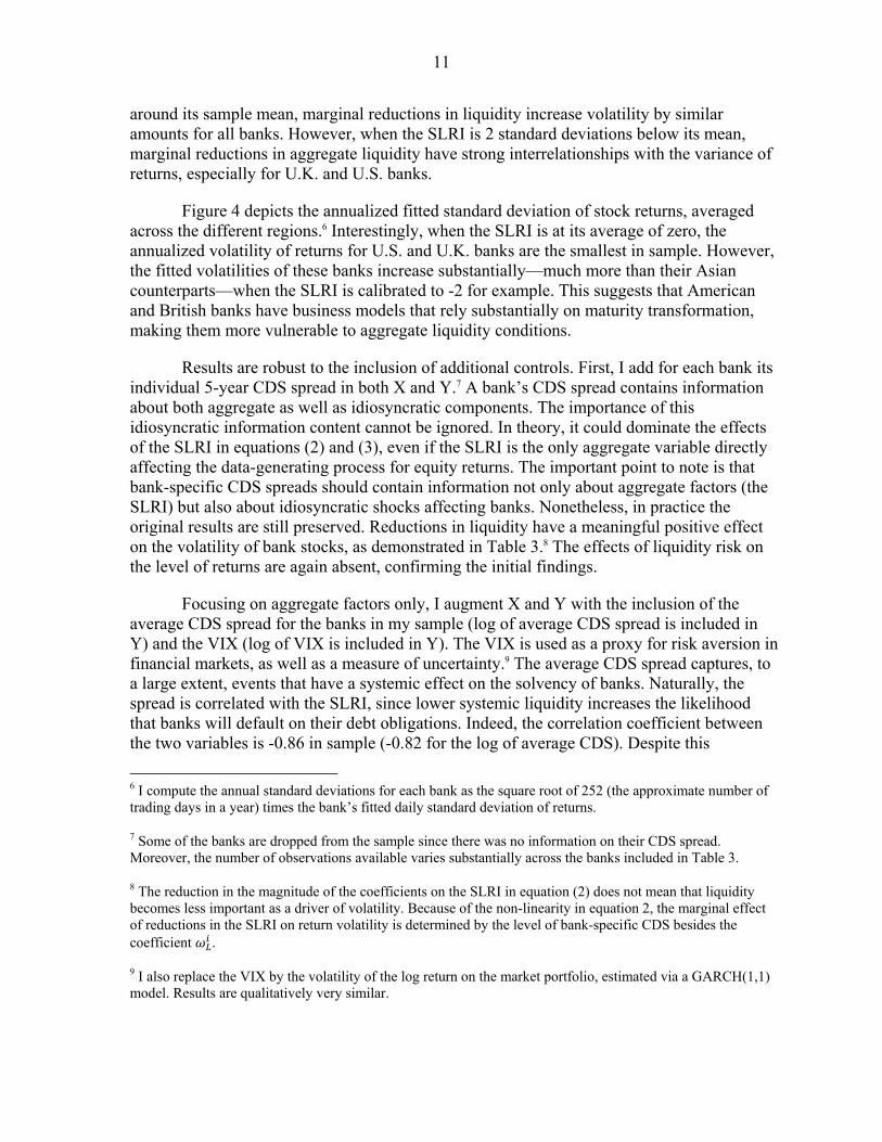
Figure 3 shows the impact of changes in the SLRI on the volatility of returns, averaged for banks across different regions. This computation is done assuming that the SLRI is at its sample average. I also consider the case where the SLRI is 2 standard deviations below its mean. As can be seen in the figure, the relationship between liquidity and bank volatility is meaningful, particularly when liquidity is scarce. When the SLRI is

5 Results are robust to several alternative specifications, like a GARCH (1, 1) or asymmetric versions of the GARCH family, like the E-GARCH, J-GARCH, etc.

11

around its sample mean, marginal reductions in liquidity increase volatility by similar amounts for all banks. However, when the SLRI is 2 standard deviations below its mean, marginal reductions in aggregate liquidity have strong interrelationships with the variance of returns, especially for U.K. and U.S. banks.

Figure 4 depicts the annualized fitted standard deviation of stock returns, averaged across the different regions.6 Interestingly, when the SLRI is at its average of zero, the annualized volatility of returns for U.S. and U.K. banks are the smallest in sample. However, the fitted volatilities of these banks increase substantially—much more than their Asian counterparts—when the SLRI is calibrated to -2 for example. This suggests that American and British banks have business models that rely substantially on maturity transformation, making them more vulnerable to aggregate liquidity conditions.

Results are robust to the inclusion of additional controls. First, I add for each bank its individual 5-year CDS spread in both X and Y.7 A bank’s CDS spread contains information about both aggregate as well as idiosyncratic components. The importance of this idiosyncratic information content cannot be ignored. In theory, it could dominate the effects of the SLRI in equations (2) and (3), even if the SLRI is the only aggregate variable directly affecting the data-generating process for equity returns. The important point to note is that bank-specific CDS spreads should contain information not only about aggregate factors (the SLRI) but also about idiosyncratic shocks affecting banks. Nonetheless, in practice the original results are still preserved. Reductions in liquidity have a meaningful positive effect on the volatility of bank stocks, as demonstrated in Table 3.8 The effects of liquidity risk on the level of returns are again absent, confirming the initial findings.

Focusing on aggregate factors only, I augment X and Y with the inclusion of the average CDS spread for the banks in my sample (log of average CDS spread is included in Y) and the VIX (log of VIX is included in Y). The VIX is used as a proxy for risk aversion in financial markets, as well as a measure of uncertainty.9 The average CDS spread captures, to a large extent, events that have a systemic effect on the solvency of banks. Naturally, the spread is correlated with the SLRI, since lower systemic liquidity increases the likelihood that banks will default on their debt obligations. Indeed, the correlation coefficient between the two variables is -0.86 in sample (-0.82 for the log of average CDS). Despite this

6 I compute the annual standard deviations for each bank as the square root of 252 (the approximate number of trading days in a year) times the bank’s fitted daily standard deviation of returns.

7 Some of the banks are dropped from the sample since there was no information on their CDS spread. Moreover, the number of observations available varies substantially across the banks included in Table 3.

8 The reduction in the magnitude of the coefficients on the SLRI in equation (2) does not mean that liquidity becomes less important as a driver of volatility. Because of the non-linearity in equation 2, the marginal effect of reductions in the SLRI on return volatility is determined by the level of bank-specific CDS besides the coefficient .

9 I also replace the VIX by the volatility of the log return on the market portfolio, estimated via a GARCH(1,1) model. Results are qualitatively very similar.

12

colinearity problem, which reduces the precision of estimates and thus their significance, the estimation results still confirm the effects of systemic liquidity on the volatility of bank stocks, as illustrated in Table 4.

I also re-estimate the model including additional measures of liquidity conditions as controls in both X and Y, with the aim of testing the ability of the SLRI to improve upon the information provided by these other variables. I consider the LIBOR-OIS spread, which many authors have argued provides highly relevant information about liquidity conditions. As can be seem in Table 5, the coefficient on the SLRI in equation (2) is still strongly negative.10 Interestingly, the LIBOR-OIS spread is more capable than the SLRI to explain the volatility of bank returns for Japanese institutions, but fails to signal the increase in volatility for several European banks. One possible explanation for this fact is that the spread contains information about solvency as well as liquidity risks (Schwartz (2010), Taylor (2009)). As a consequence, I use data on the Funding and Market Liquidity Index produced by the IMF instead.11 I denote this alternative liquidity indicator as IMF_LIQ in Table 5. The results indicate that the SLRI is still strongly correlated with equity volatility for all but a few Asian banks. Finally, I include the average CDS spread on the banking sector in addtition to IMF_LIQ as controls in both X and Y but, as seen in Table 6, the basic results are still valid: the SLRI provides useful information about the performance of banks in addition to the information contained in traditional measures of solvency and liquidity risk.

B. Portfolios of Banks

The previous analysis indicates that the SLRI has a statistically significant and

economically meaningful effect on the volatility of banks’ stock returns.12 In addition, I have shown that this effect is more pronounced for U.K. and U.S. banks relative to Asian institutions, for example. From a policy perspective, though, it would be most desirable to identify which banks’ characteristics, beyond geographic location, are determinant to their exposure to systemic liquidity risk. Ultimately, the aim is to find measures that derive from banks’ choices that indicate the risks they incur when liquidity is scarce.

With this objective in mind, I form portfolios of banks according to two different characteristics: size (proxied by market capitalization) and structural funding gaps (proxied by NSFR).13 I then re-estimate the model represented by equations (1) and (2) for the portfolios of banks instead of using data on individual institutions. More specifically, at the beginning of each year, I sort the 53 institutions into quintiles according to a certain criterion

10 I only report the estimates for equation (2). Similarly to previous results, the alternative liquidity indexes are not correlated to the level of equity returns.

11 For details about the construction of this Index, see GFSR (2010).

12 See the results in figures 3 and 4 for an illustration of the estimated importance of changes in the SLRI on the volatility of banks’ stock returns.

13 I compute the NSFR for every bank in my sample following the steps outlined in Chapter 2 of IMF (2011).

13

(either size or NSFR). I then compute the weighted daily return for each quintile (using market capitalization as the weight) through the year, and finally re-estimate the model in equations (1) and (2).

Table 7 presents the estimates from the baseline model, when no additional controls are included in either X or Y. Results are in line with the findings for individual banks. There is virtually no relationship between the SLRI and the level of portfolio returns, either for portfolios formed on market cap or NSFR. Once again, volatility of returns is strongly affected by liquidity conditions, since the estimated for each quintile i is statistically significant and economically meaningful.

As can be seem in Figure 5, the annualized standard deviation of returns on the quintile portfolios formed on market capitalization are very similar when the SLRI is at its sample average of zero. In fact, the smallest banks in the sample seem to have slightly more volatile returns under those conditions. This relationship changes, nonetheless, when the SLRI drops 2 standard deviations below its mean, but it only becomes really pronnounced for sharper declines in liquidity, for example 4 standard deviations away from the mean. Even then, the association between sensitivity to liquidity and bank size is non-monotonic: only the very large banks seem more exposed to liquidity risk, and this becomes pronounced when liquidity conditions are rather dire.

Figure 6 illustrates the corresponding results for portfolios formed on NSFR. Surprisingly, banks in the 4th and 5th quintiles (the ones supposed to be structurally less dependant on liquidity) are in fact more sensitive to fluctuations in the SLRI. This is particularly true when liquidity conditions deteriorate sharply. Once again, results are robust to the inclusion of additional controls in the model. For example, the coefficients on the SLRI in equation (2) are still statistically significant and economically important if we include the VIX and the average CDS spread for the banks in the sample as additional controls in X and Y.

As suggested before, the puzzling relation between NSFR and exposure to systemic liquidity risk uncovered here has to be qualified. The big contractions in the SLRI depicted in Figure 2 reflect short-term stress in funding and market liquidity. The NSFR, on the other hand, is a meaure that reflects banks’ long-term, structural liquidity positions. It would certainly be more appropriate to redo this exercise using the LCR as the reference characteristic. Unfortunately, the data required to compute LCR for each bank (which includes a maturity breakdown, various asset types, and specific credit characteristics of different instruments in the balance sheet) are not readily available.

One possible joint explanation for the inability of both market capitalization and NSFR to intuitively account for the pattern of exposures would be a sort of perverse interaction between the two characteristics. Since I am rank-ordering banks based on a single characteristic at a time, it is conceivable that the joint cross-sectional distribution of these characteristics may be masking some underlying, intuitive relationship between them and the SLRI. To fully address this possibility, I would need to condition the portfolio formation process on both capitalization and NSFR together. That is, I could entertaining forming quantile portfolios of both characteristics jointly. Unfortunately, due to the small sample size

14

(with only 53 banks), this alternative is not feasible. However, there seems to be virtually no relationship between the cross sectional distributions of size and NSFR. Indeed, Figure 7 presents a scatter plot of the distribution for 2004 and 2010, the beginning and end of the sample. The evidence suggests that market capitalization and NSFR are virtually uncorrelated in the cross-section.

IV. THE COST OF LIQUIDITY INSURANCE

The empirical results indicate that systemic liquidity risk has no direct effect on the level of bank returns, but it is strongly correlated with their volatility, even controlling for other aggregate and idiosyncratic factors. This link between the SLRI and bank volatility allows me to evaluate the cost faced by public authorities—central banks in particular—for providing liquidity support to banks under distress. The technique to measure the cost of liquidity insurance derives from a simple application of the traditional contingent claims analysis (CCA), also known as the Merton model.

The basic intuition behind this approach presumes that public authorities will provide the necessary support to prevent the collapse of financial firms if systemic shocks threaten the survival of large parts of the financial system. Implicitly, it is presumed that public authorities will ultimately bail-out the financial sector, assuming responsibility for its liabilities and taking ownership of the assets of failed banks. This means, essentially, that the public sector provides an implicit guarantee on bank debt, which can be modeled as a put option on bank assets with strike price and maturity determined the characteristics of the corresponding liabilities.

The market value of such put indicates the cost faced by public authorities for supporting distressed banks. To compute this measure directly, it would be necessary to observe details about the distribution of the value of a bank’s assets. Such information is usually not readily available, since a large chunk of bank assets are not priced frequently in centralized markets. Merton’s unique insight was to use information on bank’s traded liabilities together with the characterisitics of its debt to back out the unobserved parameters of the distribution of its assets. After uncovering the asset distribution, simple option pricing formulas allow for the calculation of the value of public guarantees—for different applications of this approach, see Merton (1977), Gray et al. (2006), Gray and Jobst (2010), and Gray et al. (2010).

As shown below, one of the key observables used to compute the asset distribution and the corresponding value of the implicit put is the volatility of bank equity. Now, because the empirical results have shown that bank equity volatility is directly related to the SLRI, I can use the CCA approach to measure by how much the value of the put changes as a result of fluctuations in the SLRI. This difference in the value of public guarantees forms the basis for pricing the cost of liquidity insurance. In what follows, I provide a brief overview of the CCA approach, and how to apply it in combination with the empirical results to calculate the liquidity insurance premium.

15

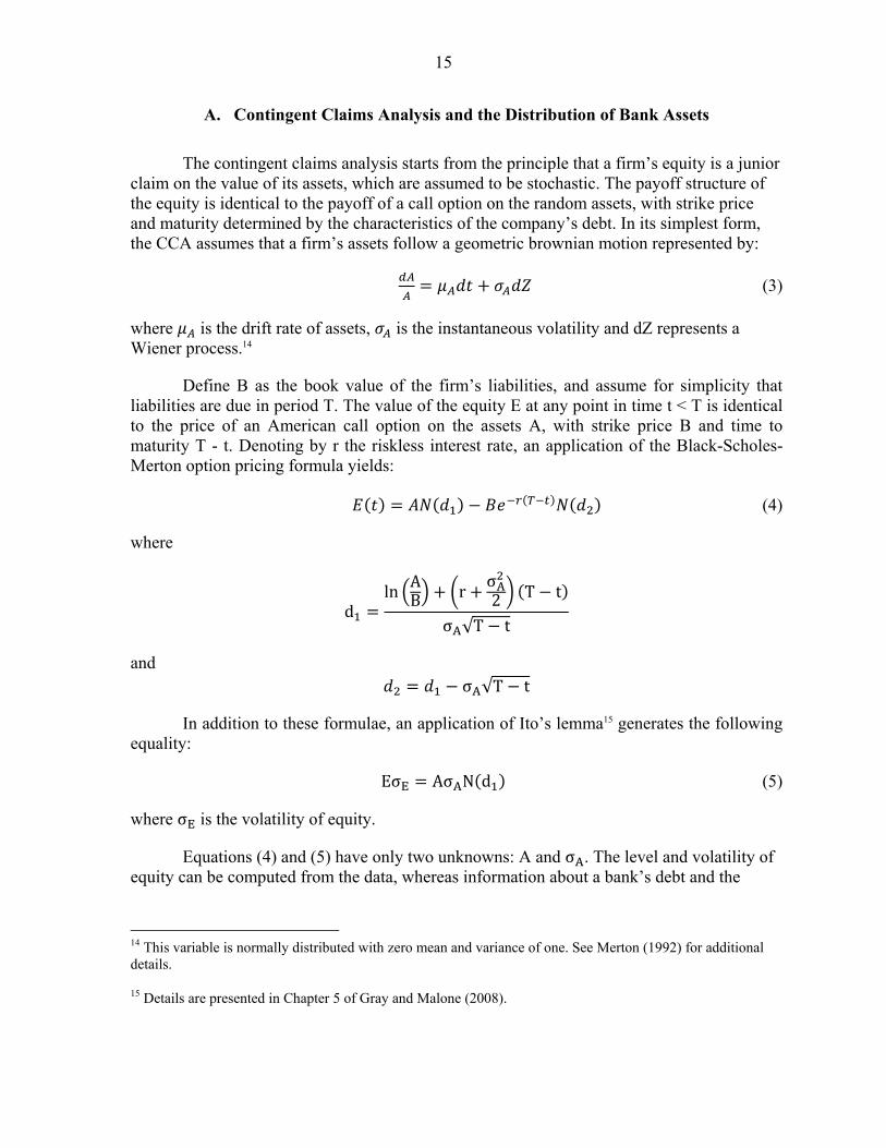
A. Contingent Claims Analysis and the Distribution of Bank Assets

The contingent claims analysis starts from the principle that a firm’s equity is a junior

claim on the value of its assets, which are assumed to be stochastic. The payoff structure of the equity is identical to the payoff of a call option on the random assets, with strike price and maturity determined by the characteristics of the company’s debt. In its simplest form, the CCA assumes that a firm’s assets follow a geometric brownian motion represented by:

(3)

where is the drift rate of assets, is the instantaneous volatility and dZ represents a Wiener process.14

Define B as the book value of the firm’s liabilities, and assume for simplicity that liabilities are due in period T. The value of the equity E at any point in time t < T is identical to the price of an American call option on the assets A, with strike price B and time to maturity T - t. Denoting by r the riskless interest rate, an application of the Black-Scholes-Merton option pricing formula yields:

(4)

where

dln

AB r

σA2 T t

σA√T t

and σA√T t

In addition to these formulae, an application of Ito’s lemma15 generates the following equality:

EσE AσAN d (5)

where σE is the volatility of equity.

Equations (4) and (5) have only two unknowns: A and σA. The level and volatility of equity can be computed from the data, whereas information about a bank’s debt and the

14 This variable is normally distributed with zero mean and variance of one. See Merton (1992) for additional details.

15 Details are presented in Chapter 5 of Gray and Malone (2008).

16

riskless interest rates can be easily uncovered. Hence, the two equations can be combined to pin down the parameters of the distribution of bank assets.

B. Systemic Liquidity Risk and the Valuation of Implicit Guarantees The basic CCA approach presented above can be extended in various directions. For the purposes of this paper, I analyze the case where the level and volatility of bank assets, A and σA, vary over time. Incorporating time variation in the data generating process for bank assets allows me to explicitly link the systemic liquidity risk indicator to the value of implicit public guarantees, and to calculate by how such guarantees change as liquidity vanishes. The key insight here is to assume that the unconditional distribution of bank assets results from a mixture of lognormal distributions, and to connect the prevalence of each specific lognormal distribution at a certain point in time to the realization of aggregate liquidity conditions. Under these assumptions, one can price the value of the implicit put conditional on a given realization of the aggregate liquidity risk factor.

More specifically, the CCA uses information on the volatility of equity combined with characteristics of a company’s debt to back out the unobserved distribution of the value of its assets. The econometric results indicate that changes in the SLRI affect the measured volatility of banks’ stocks—but not their level. Hence, if I were to apply the CCA to back out the distribution of a bank’s assets and calculate the corresponding price of the implicit put, the results would depend highly on the specific realization of the liquidity index at the time of the calculation. In other words, the price of the implicit guarantee given to each bank will be directly dependent on the realization of the liquidity index. Hence, fluctuations in liquidity impose a cost on the providers of such guarantee, and, under certain assumptions, I can precisely measure the magnitude of this cost.

To formalize this idea, I assume that, at any given point in time, the distribution of bank assets can be governed by S different lognormally distributed random variables, which are generally characterized by:

, , exp σA2

σA ε√t

where ε has a standard normal distribution. Because public support can be modeled as an implicit put option, the value of such a guarantee conditional on the realization of each process for assets is given by the Black-Scholes expression for the price of an American put:

, , , (6)

where , and , are defined as before, depending on , and σA .

Interestingly, the unconditional value of the put for a mixture of lognormals is the mixture of the individual puts. That is, the unconditional price of public guarantees on bank liabilities is given by:

 ∑ (7)

17

where is the probability of realization of each process. More importantly, changes in the value of the implicit guarantees due to different realizations of the asset process are simply given by the difference in the value of individual puts.

Finally, I assume the SLRI is an underlying factor that induces the realization of different processes for bank assets.16 For example, a high SLRI indicates periods of normalcy, where liquidity is abundant and the financial sector is stable. Under these circunstances, a bank’s assets are expected to be high and their volatility small. That is, the asset process is characterized by a lognormal distribution with initial asset level , and volatility σAL, where the subscript L denotes a “liquidity” state. If markets become illiquid— if the SLRI is low—however, the assets are expected to evolve according to a lognormal distribution with initial value , and volatility σAI.

17 Naturally, based on the empirical analysis, the underlying presumption is that , , and σAL σAL. The different pairs of parameters induce alternative values for the individual implicit puts. Hence, alternative paths for the SLRI will induce different costs faced by public authorities, providing a clear benchmark for the price of liquidity insurance.

C. Computing the Liquidity Insurance Premium

I now connect the logic outlined above with the empirical findings to present a practical example on how to calculate the liquidity insurance premium that each individual bank could face in order to pre-pay for the benefit of relying on public support.18 For simplicity, I estimate a stylized version of the heteroskedastic model represented by (1) and (2). That is, I assume that the equity return for each bank evolves according to:

  (8)

exp   1 (9)

where

~ 0,1

As before , , represent bank-specific parameters.

The model in (8) and (9) assumes that the mean equity return is constant, and that its volatility is driven solely by the SLRI and a white noise component. These assumptions

16 It may not be the single factor driving the realization of alternative lognormals.

17 As it is well known, the drift in the growth rate of assets is not important since it does not affect directly the price of options according to the Black-Scholes formula.

18 For illustration purposes, this section assumes that there are only two possible states of the world, a liquid and an illiquid state.

18

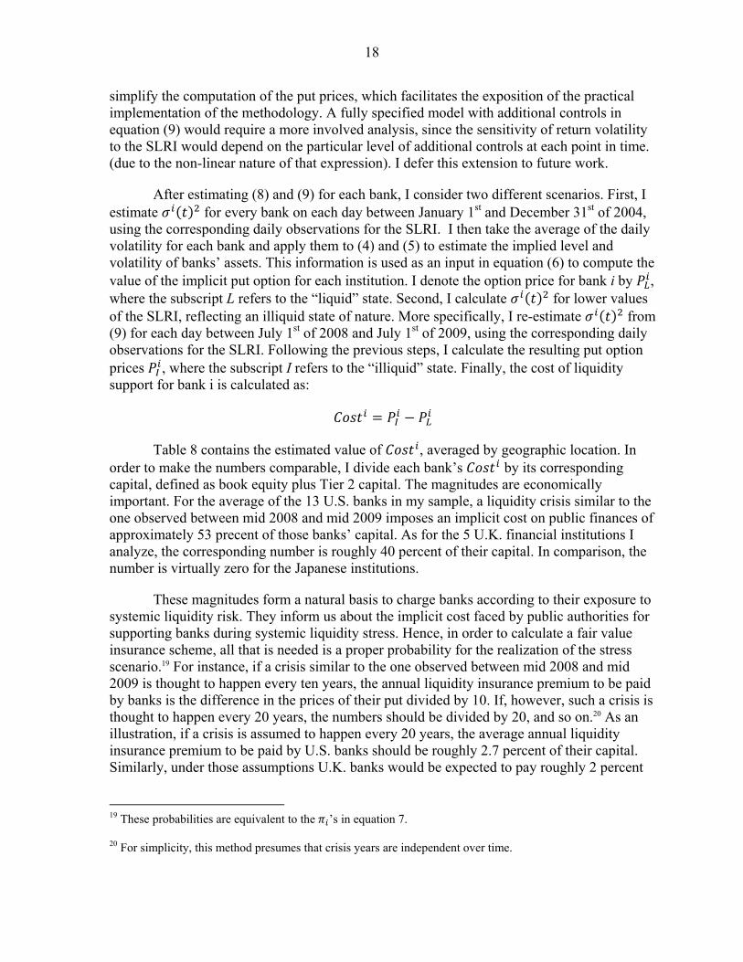
simplify the computation of the put prices, which facilitates the exposition of the practical implementation of the methodology. A fully specified model with additional controls in equation (9) would require a more involved analysis, since the sensitivity of return volatility to the SLRI would depend on the particular level of additional controls at each point in time. (due to the non-linear nature of that expression). I defer this extension to future work.

After estimating (8) and (9) for each bank, I consider two different scenarios. First, I estimate for every bank on each day between January 1st and December 31st of 2004, using the corresponding daily observations for the SLRI. I then take the average of the daily volatility for each bank and apply them to (4) and (5) to estimate the implied level and volatility of banks’ assets. This information is used as an input in equation (6) to compute the value of the implicit put option for each institution. I denote the option price for bank i by , where the subscript L refers to the “liquid” state. Second, I calculate for lower values of the SLRI, reflecting an illiquid state of nature. More specifically, I re-estimate from (9) for each day between July 1st of 2008 and July 1st of 2009, using the corresponding daily observations for the SLRI. Following the previous steps, I calculate the resulting put option prices , where the subscript I refers to the “illiquid” state. Finally, the cost of liquidity support for bank i is calculated as:

Table 8 contains the estimated value of , averaged by geographic location. In order to make the numbers comparable, I divide each bank’s by its corresponding capital, defined as book equity plus Tier 2 capital. The magnitudes are economically important. For the average of the 13 U.S. banks in my sample, a liquidity crisis similar to the one observed between mid 2008 and mid 2009 imposes an implicit cost on public finances of approximately 53 precent of those banks’ capital. As for the 5 U.K. financial institutions I analyze, the corresponding number is roughly 40 percent of their capital. In comparison, the number is virtually zero for the Japanese institutions.

These magnitudes form a natural basis to charge banks according to their exposure to systemic liquidity risk. They inform us about the implicit cost faced by public authorities for supporting banks during systemic liquidity stress. Hence, in order to calculate a fair value insurance scheme, all that is needed is a proper probability for the realization of the stress scenario.19 For instance, if a crisis similar to the one observed between mid 2008 and mid 2009 is thought to happen every ten years, the annual liquidity insurance premium to be paid by banks is the difference in the prices of their put divided by 10. If, however, such a crisis is thought to happen every 20 years, the numbers should be divided by 20, and so on.20 As an illustration, if a crisis is assumed to happen every 20 years, the average annual liquidity insurance premium to be paid by U.S. banks should be roughly 2.7 percent of their capital. Similarly, under those assumptions U.K. banks would be expected to pay roughly 2 percent

19 These probabilities are equivalent to the ’s in equation 7.

20 For simplicity, this method presumes that crisis years are independent over time.

19

of their capital on a yearly basis. For the entire sample, the average annual liquidity insurance premium is 0.81 percent of bank capital for a 1 in 20 probability of crisis.

Naturally, one can adjust such probabilities up or down to account for society’s risk aversion or to collect enough for very adverse scenarios if necessary. More interestingly, the methodology is flexible enough to allow regulators to construct alternative scenarios with regards to liquidity conditions, and compute the potential costs faced by central banks and governments. The tractability and ease of computation of the model make it a valuable tool for the quick assesment of the potential costs of disruptions in funding markets.

There are, of course, numerous limitations of the approach proposed here. First, being a reduced form model, it cannot account for the fact that the estimated parameters and sensitivities shall change upon the implementation of different regulatory policies. This, in fact, might help explain the small estimated cost of public support for European banks as illustrated in Table 8, since many of these institutions benefited from public liquidity support since the early stages of the crisis (and many continue to do so). This shortcoming can be partially addressed by re-estimating the parameters of the model relatively frequently, or by excluding from the sample periods in which active liquidity support is in place. Second, the current exposition sheds little light on why certain banks are more exposed to the SLRI than others, an important question from the perspective of bank regulation. As seen before, the relation between size and/or NSFR and exposure to the SLRI is either not very strong or counterintuitive. Additional research based on more detailed information about bank characteristics may be helpful in this respect.

Finally, it is important to mention that there are alternative ways to calculate the value of the implicit puts upon a liquidity shock. One possibility is to compute the average value of the SLRI during a stress period21, substitute it in equation (9) and then proceed with the application of equations (4), (5), and (6) to calculate the value of the implicit put during a stress period. This amounts to compute the stock price volatility at the average value of SLRI during a crisis. I do not follow this approach, though, since it ignores the non-linearity in the relation between the SLRI and stock volatility represented in equation (9). Another alternative is to compute a different value for the implicity put on each day, based on the estimated stock volatility derived from the daily realizations of the SLRI. One can then take the average of the put values during the stress period. This, however, subjects the methodology to the “noise” in the estimates of the SLRI, which tend to be short lived in many cases. Such noise may be problematic not only due to the non-linearity in the expression for volatility, but also because the option pricing formulas are also highly non-linear.

V. CONCLUSION

The evaporation of liquidity in securities and funding markets during the recent financial crisis and the resulting turmoil among financial intermediaries provides a

21 For example, the average SLRI between July 1st of 2008 and July 1st of 2009 is -1.77.

20

compelling reason for academics and policymakers to monitor systemic liquidity risk closely. The present paper attempts to contribute to this area by developing an indicator of liquidity conditions in global markets, and suggesting a methodology to assess the degree to which institutions’ are exposed to this aggregate risk factor.

One of the main virtues of the approach proposed here is its simplicity, relying on

basic economic reasoning and simple computations. Such simplicity is, notwithstanding, a source of important limitations. For instance, the reduced form nature of the modeling prevents a proper assessment of the impact of alternative policies and regulations on risk exposures. Moreover, it gives little indication about the main causes for the materialization of systemic liquidity risk and banks’ exposure to it. For instance, a bank may be charged a large sum for a risk they cannot offset by taking different decisions about their activities since they cannot be decipher why their charge is so high. Clearly, a lot more work is due before a solid framework for measuring and mitigating liquidity risk can be put in place.

First, it would be most desirable to sharpen the empirical model by conducting

additional robustness exercises and extending its application to other financial intermediaries like hedge funds or insurance companies. In the case of hedge funds or money market mutual funds, for example, one can use the evolution of net asset values as a measure of performance, instead of stock returns. Second, additional exercises should delve further on the cross-section dispersion of bank characteristics and their association with exposure to indexes like the SLRI. Finally, an important open question is why only the volatility but not the level of stock returns is systematically affected by the SLRI. These issues may guide future work on the topic of systemic liquidity risk.

21

REFERENCES Akerlof, G. A., 1970. "The Market for 'Lemons': Quality Uncertainty and the Market

Mechanism". Quarterly Journal of Economics, Vol. 84, No. 3, pp. 488-500. Bai, J. and P. Collin-Dufresne, 2010. “The Determinants of the CDS-Bond Basis During the

Financial Crisis of 2007-2009,” (New York: Columbia University) Blanco, R., S. Brennan and I. Marsh, 2005. “An empirical analysis of the dynamic relation

between investment-grade bonds and credit default swaps,” Journal of Finance, 60, pp. 2255-81.

Brunnermeier, M., 2009. “Deciphering the Liquidity and Credit Crunch 2007-2008,” Journal of Economic Literature, pp. 77-100.

Brunnermeier, M. and M. Oehmke, 2010. “The Maturity Rat Race,” NBER Working Paper

No. 16607 (Massachusetts: National Bureau of Economic Research). Brunnermier, M. and L. Pedersen, 2009. “Market Liquidity and Funding Liquidity,” Review

of Financial Studies, Vol. 22, No. 6, pp. 2201-38. Chacko, G., S. Das and R. Fan, 2010. “An Index-Based Measure of Liquidity,” Working

Paper (California: Santa Clara University). Coffey, N., W. Hrung, and A. Sarkar, 2009. “Capital Constraints, Counterparty Risk and

Deviations from Covered Interest Parity,” Staff Report No. 393 (New York: Federal Reserve Bank of New York).

Diamond D., and P. Dybvig, 1983. “Bank Runs, Deposit Insurance, and Liquidity,” Journal of Political Economy, Vol. 91, No. 3, pp. 401-419.

Diamond, D. and R. Rajan, 2001. “Liquidity Risk, Liquidity Creation, and Financial

Fragility: A Theory of Banking,” Journal of Political Economy, Vol. 109, No. 2, pp. 287-327.

Duffie, D., 1999. “Credit Swap Valuation,” Financial Analyst Journal, 55(1), pp. 73-87.

Farhi, E. and J. Tirole, 2010. “Collective Moral Hazard, Maturity Mismatch and Systemic Bailouts”, American Economic Review, 102(1), pp. 60–93.

Garleanu, N. and L. Pedersen, 2010. “Margin-based Asset Pricing and Deviations from the

Law of One Price,” The Review of Financial Studies, Vol. 24, No. 6, pp. 1980-2022.

22

Giglio, S., 2011. “Credit Default Swap Spreads and Systemic Financial Risk,” (available at: https://sites.google.com/site/stefanogiglio/research).

__________, 2010, Global Financial Stability Report, Chapter 2, “Systemic Liquidity Risk:

Improving the Resilience of Financial Institutions and Markets,” (Washington, April). __________, 2011, Global Financial Stability Report, Chapter 2, “How to Address the

Systemic Part of Liquidity Risks,” (Washington, April). Gorton, G. and A. Metrick, 2010. “Haircuts,” Yale ICF Working Paper No. 09-15,

(Connecticut: International Center for Finance, Yale University). Gray, D. and S. Malone, 2008: “Macrofinancial Risk Analysis,” John Wiley & Sons Ltd. Gray, D., R. C. Merton, and Z. Bodie, 2006. “A New Framework for Analyzing and

Managing Macrofinancial Risks,” NBER Working Paper No. 12637 (Massachusetts: National Bureau of Economic Research).

Gray, D. and A. Jobst (2010). “New Directions in Financial Sector and Sovereign Risk

Management,” Journal of Investment Management, Vol. 8, No. 1, pp. 23-38. Gray, D., A. Jobst, and S. Malone, 2010. “Quantifying Systemic Risk and Reconceptualizing

the Role of Finance for Economic Growth,” Journal of Investment Management, Vol. 8, No. 2, pp. 90-110.

Griffoli, T. and A. Ranaldo, 2010. “Limits to arbitrage during the crisis: funding liquidity

constraints and covered interest parity,” Working Paper No. 2010-14 (Switzerland: Swiss National Bank)

Hui, C., H. Genberg and T. Chung, 2009. “Funding Liquidity Risk and Deviations from Interest-Rate Parity During the Financial Crisis of 2007-2009,” Working Paper (Hong Kong: Hong Kong Monetary Authority).

Hull, J., M. Predescu and A. White, 2004. “The relationship between credit default swap spreads, bond yields, and credit rating announcements,” Journal of Banking and Finance, Vol. 28, pp. 2789-2877.

Merton, R. C., 1974: “On the Pricing of Corporate Debt: The Risk Structure of Interest Rates,” Journal of Finance, Vol. 29, pp. 449-70.

Merton, R. C., 1977: “An Analytic derivation of the Cost of Deposit Insurance on Loan Guarantees: An Application of Modern Option Pricing Theory,” Journal of Banking and Finance, Vol. 1, pp. 3-11.

23

Merton, R. C., 1992: “Continuous-Time Finance,” Blackwell Publishing.

Mitchell, M. and T. Pulvino, 2010. “Arbitrage Crashes and the Speed of Capital,” Journal of Financial Economics, Vol. 104, No. 3, pp. 469-490.

Subrahmanyam, M., A. Nashikkar, and S. Mahanti, 2009. “Limited Arbitrage and Liquidity in the Market for Credit Risk,” Working Paper No. FIN-08-011(New York: New York University).

Schwarz, K., 2010. “Mind the Gap: Disentangling Credit and Liquidity in Risk Spreads,” Working Paper Series (Pennsylvania: Wharton School of the University of Pennsylvania).

Taylor, J. and J. Williams (2008): “A Black Swan in the Money Market,” Working Paper. 2009, Vol. 1, No. 1, pages 58-83, (California: Standford University).

24

FIGURES

0

5

10

15

20

25

30

35

40

45

1 2 3 4 5 6 7 8 9 10

Pe

rce

nta

ge o

f To

tal V

aria

tio

n E

xpla

ine

d

Factor

Sources: Bloomberg L.P.; Datastream; and IMF staff estimates.

Figure 1. Principal Component Analysis

-6

-5

-4

-3

-2

-1

0

1

2

2004 2005 2006 2007 2008 2009 2010

1 2 3

Figure 2. Systemic Liquidity Risk Index

Sources: Bloomberg L.P.; Datastream; and IMF staff estimates.Note: The vertical axis measures the number of standard deviation around the zero line. Dates of vertical lines are as follows: 1—March 14, 2008, Bear Stearns rescue; 2—September 14, 2008, Lehman Brothersfailure; and 3—April 27, 2010, Greek debt crisis.

25

0

10

20

30

40

50

60

US UK Europe Australia and New Zealand

India and Korea

Japan

Ave

rage

Imp

act

on

Var

ian

ce

Region

SLRI = 0

SLRI = -2

Figure 3. Impact of Decrease in SLRI on Variance of Daily Returns

Sources: IMF staff estimates.Note: The impact on variance is calculated as the partial derivative of the expression for the variance of each bank with respect to the SLRI, and then averaged across regions. The partial derivative is evaluated at the two different values for the liquidity index.

0

10

20

30

40

50

60

70

80

90

100

US UK Europe Australia and New Zealand

India and Korea

Japan

Ave

rage

Sta

nd

ard

De

viat

ion

Region

Figure 4. Annualized Standard Deviation of Returns

SLRI = 0

SLRI = -2

Sources: IMF staff estimates.Note: The estimated daily standard deviation for each bank is multiplied by the square root of 252, and then average by region.

26

0

20

40

60

80

100

120

140

160

1st 2nd 3rd 4th 5th

An

nu

aliz

ed

Sta

nd

ard

De

viat

ion

Quintile Portfolios

Figure 5. Volatility of Portfolios Formed on Market Capitalization

SLRI = 0

SLRI = -2

SLRI = -4

Sources: Bloomberg L.P.; Datastream; and IMF staff estimates.Note: The 1st quintile portfolio contains banks with smallest market capitalization at the beggining of each year.

0

50

100

150

200

250

1st 2nd 3rd 4th 5th

An

nu

aliz

ed

Sta

nd

ard

De

viat

ion

Quintile Portfolios

Figure 6. Volatility of Portfolios Formed on NSFR

SLRI = 0

SLRI = -2

SLRi = -4

Sources: Bloomberg L.P.; Datastream; and IMF staff estimates.Note: The 1st quintile portfolio contains banks with smallest market NSFR at the beggining of each year.

27

0

10

20

30

40

50

60

0 10 20 30 40 50 60

Dis

pe

rsio

n o

f B

anks

: NSF

R

Dispersion of Banks: Market Capitalization

Figure 7. Dispersion of Capitalization vs. NSFR

2004

2010

28

TABLES

Region Banks

Australia National Australia Bank Limited

Australia Commonwealth Bank of Australia

Europe Erste Group Bank AG

Europe Dexia

Europe KBC Group-KBC Groep NV/ KBC Groupe SA

Europe BNP Paribas

Europe Société Générale

Europe Credit Agricole CIB-Credit Agricole Corporate and Investment Bank

Europe Deutsche Bank AG

Europe Commerzbank AG

Europe National Bank of Greece SA

Europe Alpha Bank AE

Europe Piraeus Bank SA

Europe UniCredit SpA

Europe Intesa Sanpaolo

Europe Millennium bcp-Banco Comercial Português, SA

Europe Banco Espirito Santo SA

Europe Banco Santander SA

Europe Banco Bilbao Vizcaya Argentaria SA

Europe Banco Popular Espanol SA

Europe UBS AG

Europe Credit Suisse AG

Europe Nordea Bank AB (publ)

Europe Svenska Handelsbanken

Europe Swedbank AB

Europe DnB Nor ASA

Europe Danske Bank A/S

India State Bank of India

Japan Mizuho Financial Group

Japan Sumitomo Mitsui Banking Corporation

Japan Kabushiki Kaisha Mitsubishi UFJ Financial Group-Mitsubishi UFJ Financial Group Inc

Japan Chuo Mitsui Asset Trust and Banking Company Limited

Korea Woori Bank

Korea Shinhan Bank

New Zeland Australia and New Zealand Banking Group

U.K. HSBC Holdings Plc

U.K. Barclays Bank Plc

U.K. Royal Bank of Scotland Group Plc (The)

U.K. Lloyds Banking Group Plc

U.K. Standard Chartered Plc

U.S. Bank of America Corporation

U.S. JP Morgan Chase & Co.

U.S. Citigroup Inc

U.S. Wells Fargo & Company

U.S. Morgan Stanley

U.S. Goldman Sachs Group, Inc

U.S. US Bancorp

U.S. PNC Financial Services Group Inc

U.S. SunTrust Banks, Inc.

U.S. BB&T Corporation

U.S. Regions Bank

U.S. Bank of New York Mellon Corporation

U.S. State Street Corporation

Table 1. List of Banks

29

Table 2. Estimates from Baseline Model

Equation for Variance

Banks Market Return SLRI SLRI

Australia National Australia Bank Limited 0.53*** 0.03 -0.80***

Australia Commonwealth Bank of Australia 0.65*** 0.02 -0.79***

Europe Erste Group Bank AG 1.52*** -0.01 -0.88***

Europe Dexia 1.33*** 0.18*** -1.24***

Europe KBC Group 1.38*** 0.04 -1.20***

Europe BNP Paribas 1.54*** -0.02 -0.96***

Europe Société Générale 1.62*** 0.05 -0.94***

Europe Credit Agricole CIB 1.59*** -0.02 -0.85***

Europe Deutsche Bank AG 1.61*** 0.01 -0.90***

Europe Commerzbank AG 1.70*** 0.12 -0.87***

Europe National Bank of Greece SA 1.28*** 0.12 -0.79***

Europe Alpha Bank AE 1.12*** 0.11 -0.76***

Europe Piraeus Bank SA 1.17*** 0.19** -0.76***

Europe UniCredit SpA 1.35*** 0.04 -0.97***

Europe Intesa Sanpaolo 1.22*** 0.04 -0.78***

Europe Millennium bcp-Banco Comercial Português, SA 0.91*** 0.12** -0.47***

Europe Banco Espirito Santo SA 0.68*** 0.10* -0.91***

Europe Banco Santander SA 1.39*** -0.02 -0.82***

Europe Banco Bilbao Vizcaya Argentaria SA 1.38*** 0.01 -0.80***

Europe Banco Popular Espanol SA 1.16*** 0.06 -0.87***

Europe UBS AG 1.37*** 0.06 -1.04***

Europe Credit Suisse AG 1.41*** 0.02 -0.78***

Europe Nordea Bank AB (publ) 1.41*** 0.02 -0.83***

Europe Svenska Handelsbanken 1.24*** -0.04 -0.78***

Europe Swedbank AB 1.51*** -0.02 -0.98***

Europe DnB Nor ASA 1.16*** -0.01 -0.95***

Europe Danske Bank A/S 1.04*** 0.01 -0.88***

India State Bank of India 0.84*** 0.07 -0.26***

Japan Mizuho Financial Group 0.55*** 0.13* -0.53***

Japan Sumitomo Mitsui Banking Corporation 0.50*** 0.08 -0.57***

Japan Mitsubishi UFJ Financial Group Inc 1.40*** -0.01 -0.34***

Japan Chuo Mitsui Asset Trust and Banking Company 0.61*** 0.08 -0.43***

Korea Woori Bank 0.68*** 0.07 -0.39***

Korea Shinhan Bank 0.92*** 0.11 -0.58***

New Zeland Australia and New Zealand Banking Group 0.62*** -0.01 -0.81***

U.K. HSBC Holdings Plc 0.97*** -0.03 -1.07***

U.K. Barclays Bank Plc 1.48*** -0.06 -1.14***

U.K. Royal Bank of Scotland Group 1.32*** -0.17** -1.27***

U.K. Lloyds Banking Group Plc 1.26*** -0.03 -1.56***

U.K. Standard Chartered Plc 1.54*** -0.04 -0.83***

U.S. Bank of America Corporation 1.11*** 0.21*** -1.79***

U.S. JP Morgan Chase & Co. 1.39*** -0.02 -1.24***

U.S. Citigroup Inc 1.36*** 0.08 -1.62***

U.S. Wells Fargo & Company 1.1*** -0.9 -1.59***

U.S. Morgan Stanley 1.78*** 0.05 -1.06***

U.S. Goldman Sachs Group, Inc 1.59*** 0.02 -0.81***

U.S. US Bancorp 1.04*** -0.06 -1.35***

U.S. PNC Financial Services Group Inc 1.13*** -0.02 -1.49***

U.S. SunTrust Banks, Inc. 1.21*** 0.01 -1.59***

U.S. BB&T Corporation 1.16*** -0.06 -1.27***

U.S. Regions Bank 1.28*** 0.07 -1.61***

U.S. Bank of New York Mellon Corporation 1.42*** 0.02 -0.95***

U.S. State Street Corporation 1.46*** 0.02 -1.43***

Equation for Level

Parameters

Note: * p-value below 10% ** p-value below 5% *** p-value below 1%

30

Table 3. Controlling for Bank Specific CDS Spread

Banks Market Return Individual CDS SLRI Individual CDS SLRI

National Australia Bank Limited 0.52*** -0.005** -0.24* 0.011*** -0.35***

Commonwealth Bank of Australia 0.62*** 0.001 0.06 0.013*** -0.26***

Erste Group Bank AG 2.19*** 0.005 0.11 0.003*** -0.80***

Dexia 1.72*** 0.125 0.13 -0.891*** -0.94***

BNP Paribas 1.52*** 0.002 0.07 0.005*** -0.83***

Société Générale 1.56*** -0.001 0.01 0.011*** -0.53***

Credit Agricole CIB 1.53*** -0.001 -0.07 0.007*** -0.62***

Deutsche Bank AG 1.61*** -0.001 -0.02 0.004** -0.76***

Commerzbank AG 1.70*** -0.001 0.10 0.002*** -0.80***

National Bank of Greece SA 1.26*** -0.001 0.03 0.001*** -0.62***

Alpha Bank AE 1.06*** -0.001 0.08 0.002*** -0.48***

Piraeus Bank SA 1.21*** -0.001 0.04 0.001*** -0.41***

UniCredit SpA 1.90*** -0.001 0.05 0.003** -0.86***

Intesa Sanpaolo 1.32*** 0.002 0.11 0.009*** -0.61***

Banco Comercial Português, SA 0.88*** -0.001 0.08 0.001*** -0.40***

Banco Espirito Santo SA 0.62*** -0.001 0.08 0.003*** -0.70***

Banco Santander SA 1.51*** -0.001 0.03 0.009*** -0.47***

Banco Bilbao Vizcaya Argentaria SA 1.34*** -0.001 -0.02 0.006*** -0.54***

Banco Popular Espanol SA 1.08*** 0.001 0.17 0.006*** -0.26***

UBS AG 1.33*** -0.001 -0.01 0.012*** -0.26***

Credit Suisse AG 1.63*** 0.003 0.07 0.005*** -0.76***

Nordea Bank AB (publ) 1.40*** 0.002 0.14 0.014*** -0.32***

Svenska Handelsbanken 1.22*** 0.001 0.02 0.012*** -0.36***

Swedbank AB 1.76*** 0.004* 0.36** 0.007*** -0.31***

DnB Nor ASA 1.32*** 0.005 0.18 0.01*** -0.54***

Danske Bank A/S 1.02*** 0.004 0.21 0.01*** -0.39***

State Bank of India 0.83*** -0.001 -0.03 0.005*** 0.16***

Mizuho Financial Group 0.55*** 0.002 0.20 0.008*** -0.26***

Sumitomo Mitsui Banking Corporation 0.49*** 0.002 0.20 -0.005*** -0.73***

Mitsubishi UFJ Financial Group Inc 1.32*** 0.002 0.04 0.001 -0.38***

Woori Bank 0.70*** -0.005 0.06 -0.010** -0.40***

Australia and New Zealand Banking Group 0.61*** -0.003 -0.18 0.013*** -0.28***

HSBC Holdings Plc 0.93*** 0.001 0.07 0.016*** -0.47***

Barclays Bank Plc 1.45*** 0.003 0.20 0.014*** -0.35***

Royal Bank of Scotland Group 1.29*** 0.001 -0.14 0.007*** -0.82***

Lloyds Banking Group Plc 1.25*** 0.003 0.25 0.003*** -1.40***

Standard Chartered Plc 1.52*** 0.003 0.15 0.006*** -0.51***

Bank of America Corporation 1.09*** .002 .45*** 0.005*** -1.49***

JP Morgan Chase & Co. 1.35*** -0.001 -0.02 0.027*** -0.16***

Citigroup Inc 1.32*** -0.002 -0.11 0.007*** -0.75***

Wells Fargo & Company 1.03*** 0.002 0.12 0.023*** -0.32***

Morgan Stanley 1.75*** -0.001 -0.15 0.007*** -0.24***

Goldman Sachs Group, Inc 1.55*** -0.001 -0.04 0.014*** 0.29***

US Bancorp 0.98*** -0.001 -0.02 0.018*** -0.44***

PNC Financial Services Group Inc 1.13*** 0.001 0.03 0.002*** -1.40***

SunTrust Banks, Inc. 1.18*** 0.002* 0.34** 0.006*** -0.94***

BB&T Corporation 1.16*** 0.002** 0.13* 0.015*** -0.29***

Bank of New York Mellon Corporation 1.56*** -0.001 0.09 0.007*** -0.60***

State Street Corporation 1.63*** -0.001 0.03 -0.009*** -1.33***

Note: * p-value below 10% ** p-value below 5% *** p-value below 1%

Equation for Level

Parameters

Equation for Variance

31

Table 4. Controlling for Average CDS Spread and VIX

Banks VIX Average CDS SLRI

National Australia Bank Limited 1.87*** 0.16** -0.01

Commonwealth Bank of Australia 2.04*** 0.18** 0.09*

Erste Group Bank AG 1.47*** -0.13* -0.40***

Dexia 1.81*** 0.24*** -0.34***

KBC Group 1.41*** 0.07 -0.60***

BNP Paribas 1.77*** -0.11* -0.37***

Société Générale 1.82*** 0.18*** -0.09

Credit Agricole CIB 1.02*** 0.23*** -0.26***

Deutsche Bank AG 1.57*** -0.01 -0.31***

Commerzbank AG 1.38*** -0.20*** -0.53***

National Bank of Greece SA 0.19 0.43*** -0.30***

Alpha Bank AE -0.35** 0.65*** -0.27***

Piraeus Bank SA 0.01 0.61*** -0.20**

UniCredit SpA 1.16*** 0.07 -0.46***

Intesa Sanpaolo 1.08*** -0.05 -0.38***

Millennium bcp-Banco Comercial Português, SA 1.47*** 0.25*** 0.27***

Banco Espirito Santo SA 0.45*** 0.56*** -0.26***

Banco Santander SA 1.49*** 0.24*** -0.02

Banco Bilbao Vizcaya Argentaria SA 1.11*** 0.19*** -0.19**

Banco Popular Espanol SA 0.92*** 0.54*** -0.01

UBS AG 1.49*** 0.20*** -0.29***

Credit Suisse AG 1.36*** -0.12* -0.38***

Nordea Bank AB (publ) 1.68*** -0.18** -0.35***

Svenska Handelsbanken 1.46*** -0.23*** -0.41***

Swedbank AB 1.38*** -0.02 -045***

DnB Nor ASA 1.75*** -0.29*** -0.51***

Danske Bank A/S 0.97*** 0.22*** -0.33***

State Bank of India 1.80*** -0.35*** 0.12**

Mizuho Financial Group 2.14*** -0.11* 0.13*

Sumitomo Mitsui Banking Corporation 1.91*** -0.23*** -0.05

Mitsubishi UFJ Financial Group Inc 1.47*** -0.17** 0.04

Chuo Mitsui Asset Trust and Banking Company 2.18*** -0.41*** 0.06

Woori Bank 1.92*** -0.59*** -0.15**

Shinhan Bank 2.13*** -0.45*** -0.16**

Australia and New Zealand Banking Group 1.92*** 0.13** 0.01

HSBC Holdings Plc 1.44*** 0.24*** -0.31***

Barclays Bank Plc 2.48*** 0.03 -0.19**

Royal Bank of Scotland Group 1.76*** 0.45*** -0.24***

Lloyds Banking Group Plc 1.42*** 0.38*** -0.58***

Standard Chartered Plc 1.67*** -0.18*** -0.32***

Bank of America Corporation 2.04*** 0.49*** -0.44***

JP Morgan Chase & Co. 2.42*** 0.15** -0.16**

Citigroup Inc 1.97*** 0-49*** -0.40***

Wells Fargo & Company 2.56*** 0.46*** -0.13*

Morgan Stanley 2.11*** -0.03 -0.29***

Goldman Sachs Group, Inc 1.54*** 0.16*** -0.07

US Bancorp 2.12*** 0.37*** -0.14**

PNC Financial Services Group Inc 2.23*** 0.23*** -0.25***

SunTrust Banks, Inc. 2.11*** 0.55*** -0.20***

BB&T Corporation 1.97*** 0.53*** -0.01

Regions Bank 2.12*** 0.64*** -0.25***

Bank of New York Mellon Corporation 1.54*** -0.20*** -0.53***

State Street Corporation 2.95*** -0.29*** -0.28***

Note: * p-value below 10% ** p-value below 5% *** p-value below 1%

Equation for Variance

32

Table 5. Controlling for Other Measures of Liquidity

Banks LIBOR-OIS SLRI IMF_LIQ SLRI

National Australia Bank Limited 0.009*** -0.41*** -0.54*** -0.39***

Commonwealth Bank of Australia 0.007*** -0.44*** -0.47*** -0.52***

Erste Group Bank AG 0.004*** -0.69*** -0.19*** -0.73***

Dexia 0.008*** -0.87*** -0.46*** -0.89***

KBC Group 0.002** -1.11*** -0.04 -1.17***

BNP Paribas 0.005*** -0.68*** -0.32*** -0.69***

Société Générale 0.006*** -0.67*** -0.37*** -0.66***

Credit Agricole CIB 0.005*** -0.61*** -0.26*** -0.64***

Deutsche Bank AG 0.004*** -0.68*** -0.19*** -0.74***

Commerzbank AG 0.004*** -0.66*** -0.22*** -0.69***

National Bank of Greece SA -0.003*** -0.95*** 0.16*** -0.93***

Alpha Bank AE -0.006*** -1.03*** 0.32*** -1.02***

Piraeus Bank SA -0.002** -0.86*** 0.12** -0.85***

UniCredit SpA 0.003*** -0.84*** -0.16*** -0.83***

Intesa Sanpaolo 0.001 -0.74*** -0.02 -0.76***

Banco Comercial Português, SA 0.007*** -0.17*** -0.41*** -0.16***

Banco Espirito Santo SA -0.001 -0.93*** -0.003 -0.91***

Banco Santander SA -0.001 -0.86*** 0.02 -0.84***

Banco Bilbao Vizcaya Argentaria SA -0.001** -0.86*** 0.05 -0.84***

Banco Popular Espanol SA 0.001 -0.83*** -0.07 -0.82***

UBS AG 0.01*** -0.60*** -0.55*** -0.63***

Credit Suisse AG 0.005*** -0.53*** -0.26*** -0.57***

Nordea Bank AB (publ) 0.004*** -0.63*** -0.20*** -0.67***

Svenska Handelsbanken 0.005*** -0.51*** -0.27*** -0.56***

Swedbank AB 0.005*** -0.77*** -0.22*** -0.82***

DnB Nor ASA 0.005*** -0.71*** -0.23*** -0.75***

Danske Bank A/S 0.002** -0.80*** -0.11** -0.79***

State Bank of India 0.008*** 0.16*** -0.44*** 0.12**

Mizuho Financial Group 0.01*** -0.03 -0.59*** -0.07*

Sumitomo Mitsui Banking Corporation 0.011*** -0.04 -0.63*** -0.06

Mitsubishi UFJ Financial Group Inc 0.004*** -0.16*** -0.22*** -0.17***

Chuo Mitsui Asset Trust and Banking Company 0.009*** 0.03 -0.47*** -0.01

Woori Bank 0.005*** -0.13*** -0.28*** -0.14***

Shinhan Bank 0.007*** -0.21*** -0.38*** -0.25***

Australia and New Zealand Banking Group 0.009*** -0.41*** -0.56*** -0.40***

HSBC Holdings Plc 0.003*** -0.92*** -0.16*** -0.95***

Barclays Bank Plc 0.01*** -0.67*** -0.60*** -0.72***

Royal Bank of Scotland Group 0.01*** -0.87*** -0.55*** -0.89***

Lloyds Banking Group Plc 0.009*** -1.15*** -0.44*** -1.22***

Standard Chartered Plc 0.009*** -0.37*** -0.51*** -0.39***

Bank of America Corporation 0.016*** -1.05*** -0.89*** -1.14***

JP Morgan Chase & Co. 0.016*** -0.52*** -0.94*** -0.54***

Citigroup Inc 0.015*** -1*** -0.82*** -1.07***

Wells Fargo & Company 0.017*** -0.85*** -0.99*** -0.91***

Morgan Stanley 0.012*** -0.53*** -0.72*** -0.54***

Goldman Sachs Group, Inc 0.008*** -0.43*** -0.53*** -0.41***

US Bancorp 0.012*** -0.80*** -0.59*** -0.91***

PNC Financial Services Group Inc 0.01*** -0.96*** -0.58*** -1***

SunTrust Banks, Inc. 0.012*** -1.04*** -0.70*** -1.09***

BB&T Corporation 0.012*** -0.76*** -0.70*** -0.79***

Regions Bank 0.014*** -1.08*** -0.80*** -1.12***

Bank of New York Mellon Corporation 0.01*** -0.52*** -0.59*** -0.50***

State Street Corporation 0.019*** -0.44*** -1.10*** -0.48***

Note: * p-value below 10% ** p-value below 5% *** p-value below 1%

Equation for Variance Equation for Variance

Parameters

33

Table 6. Controlling for Credit and Liquidity Risk

Banks Average CDS IMF_LIQ SLRI

National Australia Bank Limited 0.52*** -0.48*** -0.02

Commonwealth Bank of Australia 0.60*** -0.45*** 0.04

Erste Group Bank AG 0.34*** -0.20*** -0.53***

Dexia 0.69*** -0.42*** -0.29***KBC Group 0.38*** -0.01 -0.92***

BNP Paribas 0.42*** -0.23*** -0.44***

Société Générale 0.57*** -0.27*** -0.27***

Credit Agricole CIB 0.50*** -0.22*** -0.37***

Deutsche Bank AG 0.31*** -0.17*** -0.61***Commerzbank AG 0.16*** -0.24*** -0.59***

National Bank of Greece SA 0.46*** 0.04 -0.48***

Alpha Bank AE 0.59*** 0.14*** -0.38***

Piraeus Bank SA 0.60*** 0.07 -0.32***

UniCredit SpA 0.46*** -0.18*** -0.54***

Intesa Sanpaolo 0.28*** -0.01 -0.72***

Banco Comercial Português, SA 0.66*** -0.32*** 0.23***Banco Espirito Santo SA 0.79*** -0.14*** -0.20***

Banco Santander SA 0.45*** -0.08* -0.50***

Banco Bilbao Vizcaya Argentaria SA 0.43*** -0.07 -0.50***

Banco Popular Espanol SA 0.73*** -0.19*** -0.20***

UBS AG 0.51*** -0.43*** -0.31***

Credit Suisse AG 0.25*** -0.23*** -0.52***

Nordea Bank AB (publ) 0.24*** -0.14*** -0.61***Svenska Handelsbanken 0.17*** -0.24*** -0.58***

Swedbank AB 0.33*** -0.25*** -0.58***

DnB Nor ASA 0.14*** -0.18*** -0.79***

Danske Bank A/S 0.47*** -0.26*** -0.35***

State Bank of India 0.03 -0.42*** 0.04

Mizuho Financial Group 0.26*** -0.60*** 0.14*

Sumitomo Mitsui Banking Corporation 0.10* -0.64*** 0.04Mitsubishi UFJ Financial Group Inc 0.06 -0.39*** -0.14*

Chuo Mitsui Asset Trust and Banking Company -0.03 -0.49*** -0.05

Woori Bank -0.22*** -0.24*** -0.38***

Shinhan Bank 0.01 -0.39*** -0.28***

Australia and New Zealand Banking Group 0.52*** -0.50*** -0.01

HSBC Holdings Plc 0.70*** -0.30*** -0.34***

Barclays Bank Plc 0.64*** -0.55*** -0.21***Royal Bank of Scotland Group 0.82*** -0.76*** -0.09

Lloyds Banking Group Plc 0.74*** -0.43*** -0.46***

Standard Chartered Plc 0.29*** -0.55*** -0.25***

Bank of America Corporation 0.85*** -0.71*** -0.35***

JP Morgan Chase & Co. 0.54*** -0.74*** -0.16**Citigroup Inc 0.87*** -0.79*** -0.18***

Wells Fargo & Company 0.88*** -0.80*** -0.11*Morgan Stanley 0.27*** -0.78*** -0.26***

Goldman Sachs Group, Inc 0.23*** -0.70*** -0.13***

US Bancorp 0.89*** -0.49*** -0.14**

PNC Financial Services Group Inc 0.66*** -0.57*** -0.30***

SunTrust Banks, Inc. 0.93*** -0.60*** -0.21***BB&T Corporation 0.79*** -0.65*** -0.05

Regions Bank 0.93*** -0.64*** -0.27***

Bank of New York Mellon Corporation 0.17*** -0.65*** -0.38***

State Street Corporation 0.25*** -0.94*** -0.33***

Note: * p-value below 10% ** p-value below 5% *** p-value below 1%

Parameters: Equation for Variance

34

Table 7. Quintile Portfolios

Equation for Variance

Quintile Portfolio Market Return SLRI SLRI

1st1.29*** 0.09** -0.61***

2nd1.26*** 0.02 -1.07***

3rd1.26*** -0.01 -0.96***

4th1.38*** 0.02 -0.85***

5th1.22*** 0.01 -1.32***

1st1.32*** 0.01 -1.13***

2nd1.27*** 0.02 -0.93***

3rd1.21*** -0.01 -0.92***

4th1.22*** 0.03 -1.39***

5th1.33*** 0.02 -1.32***

Note: * p-value below 10% ** p-value below 5% *** p-value below 1%

Parameters

Equation for Level

Market

Capitalization

NSFR

Table 8. Liquidity Insurance Premium

Region Crisis Every Year Crisis Every 10 Years Crisis Every 20 Years

United States 53.20% 5.32% 2.66%

United Kingdom 39.90% 3.99% 1.99%

Europe 2.21% 0.22% 0.11%

Australia and New Zealand 0.98% 0.10% 0.05%

India and Korea 0.79% 0.08% 0.04%

Japan 0.16% 0.02% 0.01%

Annual Cost of Liquidity Insurance as a Fraction of Bank Capital

Note: Bank capital is defined as the sum of Book Equity plus Tier 2 Capital in 2009. The data was

obtained from Bankscope.