Embed Size (px)
Citation preview

The Office of Financial Research (OFR) Working Paper Series allows members of the OFR staff and their coauthors to disseminate preliminary research findings in a format intended to generate discussion and critical comments. Papers in the OFR Working Paper Series are works in progress and subject to revision. Views and opinions expressed are those of the authors and do not necessarily represent official positions or policy of the OFR or Treasury. Comments and suggestions for improvements are welcome and should be directed to the authors. OFR working papers may be quoted without additional permission.
The Difficult Business of Measuring Banks’Liquidity: Understanding the Liquidity Coverage Ratio
15-20 | October 7, 2015
Jill Cetina Office of Financial Research [email protected]
Katherine Gleason Office of Financial Research [email protected]

OFR Working Paper
October 2015
The Difficult Business of Measuring Banks’ Liquidity: Understanding the Liquidity Coverage Ratio
Jill Cetina
Katherine Gleason
Abstract In the wake of the financial crisis of 2007-09, the Basel Committee on Banking Supervision recommended bank regulators adopt a new short-term liquidity requirement, the liquidity coverage ratio (LCR), to promote greater liquidity resilience. U.S. bank regulators announced the final rule implementing that recommendation in 2014. We highlight complexities in interpreting LCRs under both Basel III and the U.S. rule when banks undertake transactions that simultaneously affect the LCR numerator and denominator, and therefore, the ratio itself. Furthermore, we show how the numerator and denominator caps in the LCR formulas introduce nonlinearities that add to the complexity of interpreting changes in the metric. LCRs calculated under the U.S. rule are more volatile and difficult to interpret than LCRs calculated under the Basel standard. This is because the U.S. rule adds a time dimension to the LCR’s volatility through inclusion of a maturity mismatch add-on term in the denominator to account for the peak-day net cash outflow during the 30-day window. Unlike some other regulatory ratios, bank supervisors, analysts, and investors need to have a clear understanding of the mechanics of LCR calculations to interpret the LCR metric, separate signal from noise, and perform informed peer analysis. In this paper, we demonstrate how the LCR is calculated under both Basel and U.S. rules to help market participants, the public, and researchers better understand this new liquidity metric. Keywords: Banking, funding JEL classifications: G14, G18, G21, G28. Jill Cetina ([email protected]) and Katherine Gleason ([email protected]) are at the Office of Financial Research. The views expressed in this paper are those of the authors alone and do not necessarily reflect those of the Office of Financial Research. We thank Clemens Bonner (De Nederlandsche Bank), Tiffany Eng, Gregory Feldberg (OFR), Iman van Lelyveld (De Nederlandsche Bank), and Stathis Tompaidis (OFR) for useful comments and suggestions. The authors take responsibility for any errors and welcome comments and suggestions.

1
Introduction
The financial crisis of 2007-09 revealed material liquidity risks at U.S. banks and bank
holding companies. Banks experienced loan commitment drawdowns, collateralized loan
obligation pipeline back-ups, and asset fire-sales. Credit rating downgrades pressured banks’
funding costs, funding availability, and solvency. Illiquid banks pulled funding from other banks.
In response, Federal Reserve discount window lending and special liquidity programs —
such as the Term Auction Facility, Primary Dealer Credit Facility, and Term Securities Lending
Facility — provided hundreds of billions of dollars in loans to banks and their broker-dealer
affiliates. Liquidity stress was not limited to U.S. banks; European banks’ U.S. branches and
subsidiaries were some of the largest beneficiaries of Federal Reserve lending. Additionally,
European banks borrowed in dollars from the Federal Reserve-European Central Bank swap line,
and in euros from the European Central Bank.
Post-crisis, the Basel Committee on Banking Supervision sought to address liquidity risk
through the development of a more rigorous standard that included the first quantitative liquidity
regulation for banks since the introduction of reserve requirements. The Basel Committee
introduced the Liquidity Coverage Ratio (LCR) to measure and limit a bank’s liquidity risk over
30 days as well as a longer-term liquidity metric, the Net Stable Funding Ratio, to measure and
limit banks’ structural asset and liability mismatches. This paper is about the first of these
measures, the LCR.
The Basel Committee finalized its LCR rule in January 2013. U.S. regulators released their
final version in September 2014. The LCR will be fully phased in by January 2017 in the United
States. Eurozone banks must comply with the LCR under Capital Requirements Directive IV, the
European Union’s implementation of Basel III, by January 2018.

2
A key initial impetus behind the development of the LCR was a desire to adopt a quantitative
minimum liquidity requirement comparable across banks because of the fragile liquidity
positions exhibited by a number of banks during the 2007-09 crisis. This goal is reflected in the
final U.S. rule, which states “the LCR is intended to be a standardized liquidity metric, designed
to promote a consistent and comparable view of the liquidity of covered companies.”1 However,
the final U.S. rule intentionally departs from the Basel III standard to prevent banks from
manipulating their LCRs in ways arguably not fully addressed by the Basel standard. It states
“the proposed [and final] unwind methodology was intended to prevent a covered company from
manipulating the composition of its HQLA amount by engaging in transactions such as
repurchase or reverse repurchase agreements that could ultimately unwind within the 30
calendar-day stress period.”2
Differences in LCR computation among jurisdictions make it difficult to compare liquidity
risk across banks. Moreover, a feature of the U.S. rule complicates assessment of liquidity risk
changes at the same bank over time. Although it is tempting to grab a set of banks’ LCR data and
draw conclusions about their — and the financial system’s — short-term liquidity risk, the
calculation of the ratio is complex and can pose challenges to such analysis.
Possible misinterpretation of the LCR is an important systemic risk issue because of potential
negative signaling effects associated with public disclosures of LCRs, particularly when they
drop below the minimum required ratio of 100 percent. Such disclosures could exacerbate, or
even start, systemic liquidity stress events. U.S. regulators acknowledged those concerns in the
final rule, noting that “other than any public disclosure requirements that may be proposed in a
separate notice, reports to the agencies of any decline in a covered company’s LCR below 100 1 See OCC and others (2014), p. 61473. 2 Ibid.

3
percent and any related supervisory actions would be considered and treated as confidential
supervisory information.”3 However, the Federal Reserve, OCC, and FDIC are not the only
organizations, federal or otherwise, imposing disclosure requirements. It remains to be seen
whether disclosure requirements under securities laws or stock exchange listing rules compel
banks to publicize LCRs below 100 percent or the adoption of associated remediation plans.4
Such public disclosures could make it more costly for a bank to sell liquid assets or take other
measures to improve its LCR during times of stress.
These concerns about public disclosure are borne out by the literature on externalities in
financial reporting. Ross (1979), Grossman (1981), and Milgrom (1981) show that firms disclose
negative information, whether required or not, since no news will be regarded as bad news. Their
findings imply banks will publicly disclose their LCRs, whether required or not.
Bankers have also expressed concerns about negative externalities associated with LCR
disclosure. For example, in JPMorgan Chase’s 2014 Annual Report, CEO Jamie Dimon suggests
that “banks and their boards of directors will be very reluctant to allow a liquidity coverage ratio
below 100 (percent) — even if the regulators say it is okay. And, in particular, no bank will want
to be the first institution to report a liquidity coverage ratio below 100 (percent) for fear of
looking weak.” Indeed, Griffin (1977) shows that the first company to disclose a problem
affecting others in its industry suffers the most in terms of stock price volatility.
3 See OCC and others (2014), p. 61517. 4 Disclosure requirements under securities laws generally fall under Item 303 of Regulation S-K, Management’s Discussion and Analysis of Financial Condition and Report of Operations; Item 303 of Regulation S-B, Management’s Discussion and Analysis or Plan of Operations; and Item 5 of Form 20-F, Operating and Financial Review and Prospects; and are collectively known as the Securities and Exchange Commission’s MD&A rules.

4
LCR Literature
Liquidity requirements, like capital requirements, are expected to enhance the resilience of
the banking industry during times of financial stress but at the cost of reduced credit during times
of economic expansion. The OFR’s 2014 Annual Report summarizes the findings of several
studies of the LCR’s potential effect on economic growth.5 Although estimates vary, these
studies suggest the LCR could reduce lending volumes by 3-5 percent, increase interest rates by
15-30 basis points, and reduce economic growth by anywhere between a few basis points and 3
percentage points. However, these studies date from 2011 and consider an early version of the
LCR, which the Basel Committee subsequently made less stringent in 2013. The final U.S. rule
is more restrictive than the 2013 Basel standard, so it is difficult to say anything conclusive about
the relationship between these studies and the final U.S. standard as adopted.
Concerns have also been raised in the literature about potential LCR interactions with
monetary policy, particularly in Europe. Bech and Keister (2013) model the potential effects of a
high-quality liquid assets shortfall within the banking system on a central bank’s ability to
control short-term interest rates. They find central banks must account for changes in the
relationship between the quantity of central bank reserves and market interest-rate changes and
that a combination of reduced demand for overnight funding and increased demand for term
funding tends to steepen the short end of the yield curve. Similarly, Bonner and Eijffinger (2013)
investigate borrowing in the interbank lending market by Dutch banks subject to a domestic
liquidity coverage ratio similar to the LCR. They find banks near the compliance threshold pay
more for interbank loans, particularly those with maturities beyond 30 days. Schmitz (2013)
shows how the LCR could interfere with monetary policy in the euro area. He also shows the
5 See Figure 3-7, page 52.

5
LCR could create feedback effects that make the unsecured interbank market more susceptible to
liquidity shocks.
Another important line of LCR research examines the new liquidity standard’s impact on
financial stability. Van den End and Kruidhof (2013) argue the LCR could serve as a helpful
macroprudential instrument if regulators are allowed to use discretion in how liquidity buffers
are deployed during times of stress. Conversely, Hartlage (2012) shows how the LCR’s
construction undermines financial stability by creating market distortions associated with bank
attempts to maintain compliance. His examples demonstrate a snowballing effect that could
occur when a bank attempts to roll over short-term wholesale funding subject to a 100 percent
runoff rate in the rule. Hartlage also shows that if banks attempt to avoid the problem by
substituting retail deposits for wholesale funding, aggressive competition for those deposits
among banks subject to the LCR standard could result in increased retail deposit runoff rates and
volatility across the banking sector.
There are also studies of the likely effects of the LCR on bank balance sheets.
Balasubramanyan and VanHoose (2013) present a theoretical model of bank-balance-sheet
dynamics to test how the LCR constraint is likely to affect deposits. They find mostly ambiguous
and confounding deposit dynamics given the complexity of the LCR calculation. Banerjee and
Mio (2014) empirically investigate British banks’ response to the United Kingdom’s Individual
Liquidity Guidance regulation and find evidence banks increased their nonfinancial deposits and
reduced their reliance on short-term wholesale funding.
Lastly, there are a few studies examining the relationship between various accounting
measures and the LCR. Song (2014) investigates the application of accounting rules to liquidity
regulation and finds that recurring fair value measurements have procyclical effects on the LCR.

6
Hong et al. (2014) use Call Report data to approximate the LCR and the net stable funding ratio
and find only limited effects on bank failures.
This paper contributes to the literature on the efficacy of the LCR’s ratio approach to
measuring liquidity risk. Examples demonstrate the analytical challenges in interpreting banks’
LCRs when transactions simultaneously affect the numerator and denominator. We proceed as
follows: First, we describe how the LCR is defined and calculated under the Basel rule, which
uses adjustments to remove the effects of secured funding transactions or asset exchanges. Next,
we show that even with those adjustments, there is room for manipulation of buffer
diversification requirements under the Basel rule. The U.S. rule addresses that manipulation, but
introduces the potential for significant divergence from the Basel standard that reduces
comparability across banks operating under the two different standards. The U.S. rule also
introduces volatility in reporting for the same bank over time. Under both standards, banks can
undertake secured funding transactions which affect the numerator and denominator of the LCR,
and thus, alter the ratio itself.
Computing the LCR
The LCR requires covered banks to hold sufficient high-quality liquid assets (HQLA) to
survive a significant liquidity stress scenario lasting 30 days. The most basic form of the LCR,
often used in academic papers to explain the standard to the reader, is:
𝐻𝐻𝐻𝐻𝐻𝐻𝐻𝐻
𝑛𝑛𝑛𝑛𝑛𝑛 𝑐𝑐𝑐𝑐𝑐𝑐ℎ 𝑜𝑜𝑜𝑜𝑛𝑛𝑜𝑜
𝑜𝑜𝑜𝑜𝑜𝑜 𝑜𝑜𝑜𝑜𝑛𝑛𝑜𝑜 30 𝑑𝑑𝑐𝑐𝑑𝑑𝑐𝑐≥ 100%
But there is much more to the rule than this simple summary ratio. The calculation of both
the numerator and denominator are complex and involve over 300 inputs. The Basel version
contains two caps in the LCR numerator to ensure asset diversification in banks’ HQLA buffers

7
and another cap in the denominator to prevent over-reliance on cash inflows. These caps make
use of min/max functions that introduce nonlinearities into banks’ LCRs and increase the
complexity of forecasting and maintaining compliance, particularly during liquidity shocks. The
U.S. rule contains additional min/max functions in both the numerator and denominator.
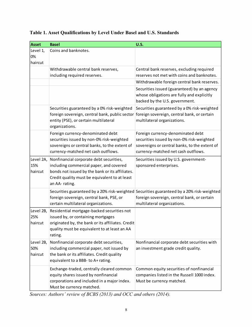
The Basel standard categorizes the types of assets that qualify as HQLA in decreasing order
of quality and liquidity. Level 1 assets are the highest quality and most liquid assets and are
included in the HQLA pool at their full market value. Level 2A assets are considered liquid,
stable, and readily marketable, but less so than Level 1 assets. As a result, Level 2A assets are
subject to a 15 percent haircut before inclusion in the HQLA pool. Level 2B assets receive
haircuts of 25 or 50 percent, depending on type, to reflect both their lower liquidity and higher
price volatility. Table 1 compares qualifying assets and haircuts under the Basel and U.S.
standards.6
The diversification caps are applied to Level 2 assets to ensure banks do not rely too much on
these less liquid assets during a time of liquidity stress. The amount of Level 2B assets allowed
in a bank’s total HQLA pool is capped at 15 percent. The amount of Level 2A and Level 2B
assets, combined, is capped at 40 percent.
6 The European Union definitions in Capital Requirements Directive IV also differ from Basel. For example, certain high-quality covered bonds are considered Level 1 assets but are subject to a 7 percent haircut.
8
Table 1. Asset Qualifications by Level Under Basel and U.S. Standards
Sources: Authors’ review of BCBS (2013) and OCC and others (2014).
Asset Basel U.S.Level 1, 0% haircut
Coins and banknotes.
Withdrawable central bank reserves, including required reserves.
Securities guaranteed by a 0% risk-weighted foreign sovereign, central bank, public sector entity (PSE), or certain multilateral organizations.Foreign currency-denominated debt securities issued by non-0% risk-weighted sovereigns or central banks, to the extent of currency-matched net cash outflows.
Central bank reserves, excluding required reserves not met with coins and banknotes.Withdrawable foreign central bank reserves.Securities issued (guaranteed) by an agency whose obligations are fully and explicitly backed by the U.S. government.
Securities guaranteed by a 0% risk-weighted foreign sovereign, central bank, or certain multilateral organizations.
Foreign currency-denominated debt securities issued by non-0% risk-weighted sovereigns or central banks, to the extent of currency-matched net cash outflows.
Level 2A, 15% haircut
Nonfinancial corporate debt securities, including commercial paper, and covered bonds not issued by the bank or its affiliates. Credit quality must be equivalent to at least an AA- rating.
Securities guaranteed by a 20% risk-weighted foreign sovereign, central bank, PSE, or certain multilateral organizations.
Securities issued by U.S. government-sponsored enterprises.
Securities guaranteed by a 20% risk-weighted foreign sovereign, central bank, or certain multilateral organizations.
Level 2B, 25% haircut
Level 2B, 50% haircut
Residential mortgage-backed securities not issued by, or containing mortgages originated by, the bank or its affiliates. Credit quality must be equivalent to at least an AA rating.
Nonfinancial corporate debt securities, including commercial paper, not issued by the bank or its affiliates. Credit quality equivalent to a BBB- to A+ rating.
Exchange-traded, centrally cleared common equity shares issued by nonfinancial corporations and included in a major index. Must be currency matched.
Nonfinancial corporate debt securities with an investment grade credit quality.
Common equity securities of nonfinancial companies listed in the Russell 1000 index. Must be currency matched.

9
LCR Manipulation: Numerator Effects Under Basel III
To prevent the bank from using secured funding transactions to circumvent the caps on the
lower quality Level 2 and Level 2B assets, the Basel rule requires adjusting a bank’s HQLA.
Adjusted Level 1, Level 2A, and Level 2B HQLA amounts are determined by unwinding all of
the bank’s secured lending and funding transactions and asset exchanges involving HQLA and
maturing within the 30-day window. These adjusted values are then used to determine the
amount of Level 2 and Level 2B HQLA excluded from the LCR numerator based on the caps.
Under the Basel rule, the formula for the LCR numerator is:
𝐻𝐻𝐻𝐻𝐻𝐻𝐻𝐻 = 𝐻𝐻1 + 𝐻𝐻2𝐻𝐻 + 𝐻𝐻2𝐵𝐵 − 𝐻𝐻2𝐵𝐵 𝑛𝑛𝑒𝑒𝑐𝑐𝑛𝑛𝑐𝑐𝑐𝑐 𝑜𝑜𝑛𝑛𝑑𝑑𝑛𝑛𝑜𝑜 15% 𝑐𝑐𝑐𝑐𝑐𝑐 − 𝐻𝐻2 𝑛𝑛𝑒𝑒𝑐𝑐𝑛𝑛𝑐𝑐𝑐𝑐 𝑜𝑜𝑛𝑛𝑑𝑑𝑛𝑛𝑜𝑜 40% 𝑐𝑐𝑐𝑐𝑐𝑐
Where,
𝐻𝐻2𝐵𝐵 𝑛𝑛𝑒𝑒𝑐𝑐𝑛𝑛𝑐𝑐𝑐𝑐 𝑜𝑜𝑛𝑛𝑑𝑑𝑛𝑛𝑜𝑜 15% 𝑐𝑐𝑐𝑐𝑐𝑐 = 𝑚𝑚𝑐𝑐𝑒𝑒 �𝐻𝐻2𝐵𝐵𝑎𝑎𝑎𝑎𝑎𝑎 −1585
× �𝐻𝐻1𝑎𝑎𝑎𝑎𝑎𝑎 + 𝐻𝐻2𝐻𝐻𝑎𝑎𝑎𝑎𝑎𝑎�, 𝐻𝐻2𝐵𝐵𝑎𝑎𝑎𝑎𝑎𝑎 − 1560
× 𝐻𝐻1𝑎𝑎𝑎𝑎𝑎𝑎 , 0�
𝐻𝐻2 𝑛𝑛𝑒𝑒𝑐𝑐𝑛𝑛𝑐𝑐𝑐𝑐 𝑜𝑜𝑛𝑛𝑑𝑑𝑛𝑛𝑜𝑜 40% 𝑐𝑐𝑐𝑐𝑐𝑐
= 𝑚𝑚𝑐𝑐𝑒𝑒 �(𝐻𝐻2𝐻𝐻𝑎𝑎𝑎𝑎𝑎𝑎 + 𝐻𝐻2𝐵𝐵𝑎𝑎𝑎𝑎𝑎𝑎 − 𝐻𝐻2𝐵𝐵 𝑛𝑛𝑒𝑒𝑐𝑐𝑛𝑛𝑐𝑐𝑐𝑐 𝑜𝑜𝑛𝑛𝑑𝑑𝑛𝑛𝑜𝑜 15% 𝑐𝑐𝑐𝑐𝑐𝑐 ) −4060
× 𝐻𝐻1𝑎𝑎𝑎𝑎𝑎𝑎 , 0�
Our first LCR calculation example, shown in Table 2, has no HQLA adjustments. That is,
L1adj = L1, L2Aadj = L2A, and L2Badj = L2B. Subtracting the excess L2B and L2 assets from the
sum of L1, L2A, and L2B yields HQLA of $250. Because of the caps on Level 2B and Level 2
assets, $1,550 of the bank’s $1,800 in eligible HQLA is excluded from the LCR numerator.
Clearly, the bank has an incentive to exchange Level 2B assets for Level 1 and Level 2A assets
to boost the amount of HQLA in its LCR numerator.

10
Table 2. LCR Numerator with No HQLA Adjustments
HQLA Category Pre-haircut
HQLA Haircut Unadjusted
HQLA Adjusted
HQLA Level 1 150.00 0.00 150.00 150.00 Level 2A 294.12 0.15 250.00 250.00 Level 2B 2,800.00 0.50 1,400.00 1,400.00 Total 1,800.00 1,800.00 Subtraction for 15% cap 1,362.50 Subtraction for 40% cap 187.50 LCR numerator 250.00
Sources: Federal Register and authors’ data adjustments and calculations
In our second example, the bank initiates a five-day repurchase agreement (repo) and an asset
exchange backed by a total of $2,600 in Level 2B HQLA in an attempt to increase its LCR
numerator. The bank obtains $1,050 in cash, a Level 1 asset, in exchange for posting $2,100 in
Level 2B collateral. The difference between the amount of cash received and the amount of
collateral posted reflects the 50 percent haircut on the Level 2B assets. The bank exchanges
another $500 in Level 2B assets, worth $250 in cash, for $250/(1 – 0.15) = $294.12 in Level 2A
assets (pre-haircut). The bank’s unadjusted HQLA on Day 0 at the start of the 30-day LCR
calculation window is shown in the last column of Table 3. Its total unadjusted HQLA is still
$1,800, but its HQLA is now mostly higher quality Level 1 and 2A assets.
Table 3. Manipulation of HQLA Using Repo and Asset Exchange
HQLA Category
Pre-haircut HQLA Before
Repo/Exchange Repo/Exchange
Amounts
Pre-haircut HQLA After
Repo/Exchange Haircut Unadjusted
HQLA Level 1 150.00 1,050.00 1,200.00 0.00 1,200.00 Level 2A 294.12 294.12 588.24 0.15 500.00 Level 2B 2,800.00 -2,600.00 200.00 0.50 100.00 Total 1,800.00
Source: Federal Register and authors’ data adjustments and calculations
In Table 4, we use these pre- and post-repo HQLA amounts to show how the Basel rule
prevents this type of HQLA manipulation. The unadjusted Level 1, 2A, and 2B amounts in Table

11
4 match those in the last column of Table 3. When we unwind the repo and asset exchange, we
get the adjusted HQLA amounts shown in the last column of Table 4, which match those in the
last column of Table 2. The Basel calculation recognizes the cash on the bank’s balance sheet
today obtained through the repo might not be available at the end of the 30-day horizon and
gives the firm no credit for the cash as a Level 1 asset in determining whether its HQLA buffer is
diversified.7 It does so by computing the caps on Level 2A and Level 2B assets using the
adjusted HQLA amounts, which are the same amounts the bank started with before it attempted
to manipulate its HQLA.
Table 4. LCR Numerator with Repo and Asset Exchange
HQLA Category Pre-haircut
HQLA Haircut Unadjusted
HQLA Adjusted
HQLA Level 1 1,200.00 0.00 1,200.00 150.00 Level 2A 588.24 0.15 500.00 250.00 Level 2B 200.00 0.50 100.00 1,400.00 Total 1,800.00 1,800.00 Subtraction for 15% cap 1,362.50 Subtraction for 40% cap 187.50 LCR numerator 250.00
Sources: Federal Register and authors’ data adjustments and calculations
Although this calculation solves the important problem of banks using short-term repo
transactions to create the appearance of HQLA diversification, it leaves unresolved issues posed
by banks’ reverse repos. A bank could, in theory, lend out most, or even all, of its cash in a 29-
day reverse repo transaction and still receive credit under the Basel rule for its Level 2 assets
because the diversification cap applies only to the bank’s HQLA at the end of the 30-day
window. Although the bank’s cash is locked up for most of the month in a reverse repo, it is still
credited for the cash’s return on Day 29, allowing the Level 2 assets it continues to hold on its
7 See OCC and others (2014), pp. 61474-61477. We scaled the Levels 1, 2A, and 2B amounts by a factor of 100.
12
balance sheet to count as HQLA. In other words, the bank’s adjusted Level 1 amount of $1,200
under the reverse repo “uncaps” the Level 2 assets it currently holds because the reverse repo
unwinds within the 30-day window. The HQLA diversification cap under the Basel rule arguably
is not binding even though the firm’s $1,800 in HQLA consists almost solely of Level 2 assets
for most of the 30-day period.
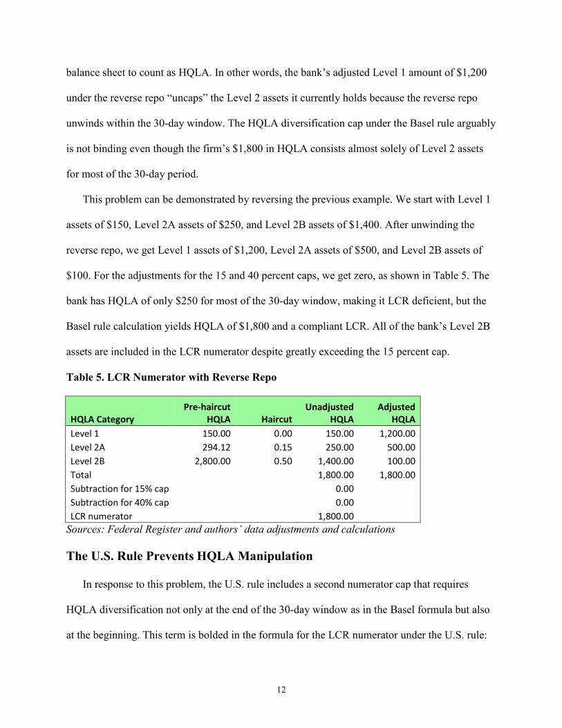
This problem can be demonstrated by reversing the previous example. We start with Level 1
assets of $150, Level 2A assets of $250, and Level 2B assets of $1,400. After unwinding the
reverse repo, we get Level 1 assets of $1,200, Level 2A assets of $500, and Level 2B assets of
$100. For the adjustments for the 15 and 40 percent caps, we get zero, as shown in Table 5. The
bank has HQLA of only $250 for most of the 30-day window, making it LCR deficient, but the
Basel rule calculation yields HQLA of $1,800 and a compliant LCR. All of the bank’s Level 2B
assets are included in the LCR numerator despite greatly exceeding the 15 percent cap.
Table 5. LCR Numerator with Reverse Repo
HQLA Category Pre-haircut
HQLA Haircut Unadjusted
HQLA Adjusted
HQLA Level 1 150.00 0.00 150.00 1,200.00 Level 2A 294.12 0.15 250.00 500.00 Level 2B 2,800.00 0.50 1,400.00 100.00 Total 1,800.00 1,800.00 Subtraction for 15% cap 0.00 Subtraction for 40% cap 0.00 LCR numerator 1,800.00
Sources: Federal Register and authors’ data adjustments and calculations
The U.S. Rule Prevents HQLA Manipulation
In response to this problem, the U.S. rule includes a second numerator cap that requires
HQLA diversification not only at the end of the 30-day window as in the Basel formula but also
at the beginning. This term is bolded in the formula for the LCR numerator under the U.S. rule:

13
𝐻𝐻𝐻𝐻𝐻𝐻𝐻𝐻 = 𝐻𝐻1 + 𝐻𝐻2𝐻𝐻 + 𝐻𝐻2𝐵𝐵 −𝑚𝑚𝑐𝑐𝑒𝑒 (𝑯𝑯𝑯𝑯𝑯𝑯𝑯𝑯 𝒆𝒆𝒆𝒆𝒆𝒆𝒆𝒆𝒆𝒆𝒆𝒆,𝐻𝐻𝐻𝐻𝐻𝐻𝐻𝐻𝑎𝑎𝑎𝑎𝑎𝑎 𝑛𝑛𝑒𝑒𝑐𝑐𝑛𝑛𝑐𝑐𝑐𝑐)
Where,
𝐻𝐻𝐻𝐻𝐻𝐻𝐻𝐻 𝑛𝑛𝑒𝑒𝑐𝑐𝑛𝑛𝑐𝑐𝑐𝑐 = 𝐻𝐻2 𝑛𝑛𝑒𝑒𝑐𝑐𝑛𝑛𝑐𝑐𝑐𝑐 + 𝐻𝐻2𝐵𝐵 𝑛𝑛𝑒𝑒𝑐𝑐𝑛𝑛𝑐𝑐𝑐𝑐
𝐻𝐻𝐻𝐻𝐻𝐻𝐻𝐻𝑎𝑎𝑎𝑎𝑎𝑎 𝑛𝑛𝑒𝑒𝑐𝑐𝑛𝑛𝑐𝑐𝑐𝑐 = 𝐻𝐻2𝑎𝑎𝑎𝑎𝑎𝑎 𝑛𝑛𝑒𝑒𝑐𝑐𝑛𝑛𝑐𝑐𝑐𝑐 + 𝐻𝐻2𝐵𝐵𝑎𝑎𝑎𝑎𝑎𝑎 𝑛𝑛𝑒𝑒𝑐𝑐𝑛𝑛𝑐𝑐𝑐𝑐
Where,
𝐻𝐻2 𝑛𝑛𝑒𝑒𝑐𝑐𝑛𝑛𝑐𝑐𝑐𝑐 = 𝑚𝑚𝑐𝑐𝑒𝑒 (𝐻𝐻2𝐻𝐻 + 𝐻𝐻2𝐵𝐵 − 0.6667 × 𝐻𝐻1,0)
𝐻𝐻2𝐵𝐵 𝑛𝑛𝑒𝑒𝑐𝑐𝑛𝑛𝑐𝑐𝑐𝑐 = 𝑚𝑚𝑐𝑐𝑒𝑒 (𝐻𝐻2𝐵𝐵 − 𝐻𝐻2 𝑛𝑛𝑒𝑒𝑐𝑐𝑛𝑛𝑐𝑐𝑐𝑐 − 0.1765 × (𝐻𝐻1 + 𝐻𝐻2𝐻𝐻), 0)
𝐻𝐻2𝑎𝑎𝑎𝑎𝑎𝑎 𝑛𝑛𝑒𝑒𝑐𝑐𝑛𝑛𝑐𝑐𝑐𝑐 = 𝑚𝑚𝑐𝑐𝑒𝑒 (𝐻𝐻2𝐻𝐻𝑎𝑎𝑎𝑎𝑎𝑎 + 𝐻𝐻2𝐵𝐵𝑎𝑎𝑎𝑎𝑎𝑎 − 0.6667 × 𝐻𝐻1𝑎𝑎𝑎𝑎𝑎𝑎 , 0)
𝐻𝐻2𝐵𝐵𝑎𝑎𝑎𝑎𝑎𝑎 𝑛𝑛𝑒𝑒𝑐𝑐𝑛𝑛𝑐𝑐𝑐𝑐 = 𝑚𝑚𝑐𝑐𝑒𝑒 (𝐻𝐻2𝐵𝐵𝑎𝑎𝑎𝑎𝑎𝑎 − 𝐻𝐻2𝑎𝑎𝑎𝑎𝑎𝑎 𝑛𝑛𝑒𝑒𝑐𝑐𝑛𝑛𝑐𝑐𝑐𝑐 − 0.1765 × �𝐻𝐻1𝑎𝑎𝑎𝑎𝑎𝑎 + 𝐻𝐻2𝐻𝐻𝑎𝑎𝑎𝑎𝑎𝑎�, 0)
Although the formulas are stated a little differently under the U.S. rule as compared to Basel,
in practice, they apply the 40 percent cap on Level 2 and 15 percent cap on Level 2B HQLA on
the unadjusted HQLA amounts measured on Day 0 and the adjusted amounts measured on Day
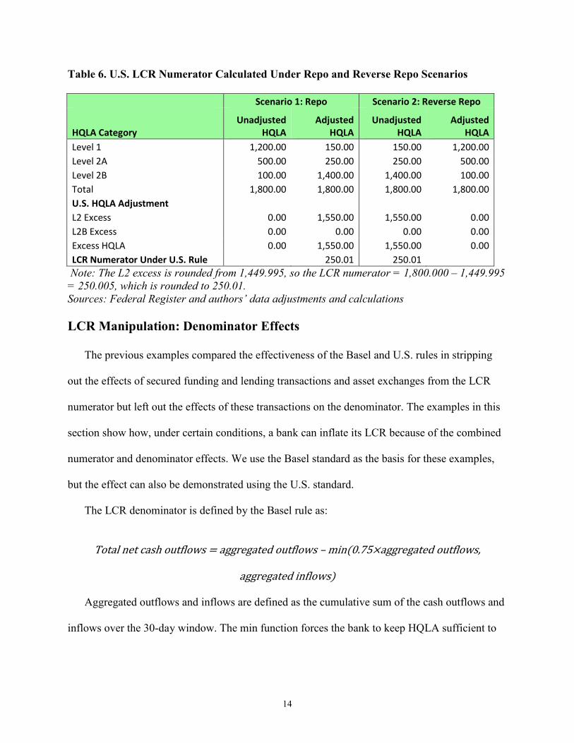
30.8 The U.S. calculation considers HQLA diversification on both Day 0 and Day 30 and avoids
potential circumvention of the HQLA diversification cap using reverse repos and repos. Table 6
shows no matter what the starting and ending HQLA amounts are for the 30-day window, the
amount of HQLA included in the LCR numerator equals $250 under the U.S. rule, avoiding the
problem of uncapping excess Level 2 assets.9
8 Rounding error differences can arise in calculations since the U.S. rule uses the approximation 0.6667 for the 40/60 ratio of Level 2 to Level 1 assets and the approximation 0.1765 for the 15/85 ratio of Level 2B to Level 1 + Level 2A assets. 9 In this example, the U.S. formula for computing the L2B excess produces the counterintuitive result of zero for the Scenario 1 adjusted HQLA amounts and the Scenario 2 unadjusted HQLA amounts because the L2 excess already fully accounts for the Level 2B excess and is subtracted to avoid double counting: max(1400 – 1550 – 0.1765 × (150 + 250), 0) = 0.
14
Table 6. U.S. LCR Numerator Calculated Under Repo and Reverse Repo Scenarios Scenario 1: Repo Scenario 2: Reverse Repo
HQLA Category Unadjusted
HQLA Adjusted
HQLA Unadjusted
HQLA Adjusted
HQLA Level 1 1,200.00 150.00 150.00 1,200.00 Level 2A 500.00 250.00 250.00 500.00 Level 2B 100.00 1,400.00 1,400.00 100.00 Total 1,800.00 1,800.00 1,800.00 1,800.00 U.S. HQLA Adjustment
L2 Excess 0.00 1,550.00 1,550.00 0.00 L2B Excess 0.00 0.00 0.00 0.00 Excess HQLA 0.00 1,550.00 1,550.00 0.00 LCR Numerator Under U.S. Rule 250.01 250.01
Note: The L2 excess is rounded from 1,449.995, so the LCR numerator = 1,800.000 – 1,449.995 = 250.005, which is rounded to 250.01. Sources: Federal Register and authors’ data adjustments and calculations
LCR Manipulation: Denominator Effects
The previous examples compared the effectiveness of the Basel and U.S. rules in stripping
out the effects of secured funding and lending transactions and asset exchanges from the LCR
numerator but left out the effects of these transactions on the denominator. The examples in this
section show how, under certain conditions, a bank can inflate its LCR because of the combined
numerator and denominator effects. We use the Basel standard as the basis for these examples,
but the effect can also be demonstrated using the U.S. standard.
The LCR denominator is defined by the Basel rule as:
Total net cash outflows = aggregated outflows – min(0.75×aggregated outflows,
aggregated inflows)
Aggregated outflows and inflows are defined as the cumulative sum of the cash outflows and
inflows over the 30-day window. The min function forces the bank to keep HQLA sufficient to

15
meet at least 25 percent of its expected cash outflows rather than over-rely on expected cash
inflows that might not materialize during an adverse liquidity event.
The cash inflows and outflows associated with HQLA adjustments are not simply added and
subtracted from the denominator.10 In the case of repos — or similar secured funding
transactions or asset exchanges — the incoming cash is counted as Level 1 HQLA in the LCR
numerator, but it is not included as a cash inflow in the denominator because that would double
count it. However, assuming the repo matures within the 30-day LCR window, there is
potentially a cash outflow associated with the transaction to include in the LCR denominator.
The size of this cash outflow reflects the risk the bank will not be able to roll over its funding.
This rollover risk, in turn, depends on the quality of the underlying collateral. If the repo is
backed by a Level 1 asset, there is no outflow associated with the transaction. The underlying
assumption is the bank can roll over 100 percent of the short-term funding it can secure with that
collateral. If the repo is backed by a Level 2A asset, the outflow on the day the repo matures
equals 15 percent of the amount of cash borrowed. The underlying assumption is that, under
stress, the bank will only be able to roll over 85 percent (100 percent minus the 15-percent
haircut) of the short-term funding it can secure with the now-devalued collateral. For Level 2B
collateral, the outflow is 25 percent or 50 percent, depending on the underlying collateral.11
In the case of reverse repos, or similar transactions, there is no cash outflow since the cash
was already deducted from the HQLA amount in the numerator. However, similar to the
treatment of cash outflows associated with repos, the cash inflows associated with reverse repos
10 The rules for determining cash inflows and outflows are complex and differ according to Basel and U.S. rules. Details on the Basel rule can be found in BCBS (2013). Details on the U.S. rule can be found in OCC and others (2014). 11 Under the Basel standard, residential mortgage-backed securities have an assumed outflow of 25 percent of the amount borrowed while other Level 2B assets have an assumed outflow of 50 percent.

16
are tied to the haircuts applied to the underlying collateral. The haircuts reflect assumptions
about the reduction in secured lending that will occur during a time of liquidity stress. If the
collateral underlying a reverse repo is a Level 1 asset, there is no cash inflow included in the
LCR denominator calculation because it is assumed the bank will renew the agreement in full.
However, if, for example, the underlying collateral is a Level 2A asset, the bank records a cash
inflow on the day the transaction matures equal to 15 percent of the amount of cash lent. The
underlying assumption is the bank will only provide 85 percent of the cash originally lent when it
renews the agreement.
The next example demonstrates both numerator and denominator effects under a Basel rule
reverse repo scenario. We start with the pre-reverse repo HQLA values shown in Table 7,
Scenario 1. The bank’s starting LCR is 133 percent, which is well above the minimum 100
percent required for compliance. The HQLA caps are minimally binding; Level 2B assets are 15
percent of total HQLA and Level 2 assets are 40 percent of total HQLA, so none of the Level 2
assets are deducted from total HQLA. The denominator constraint is nonbinding since 75 percent
of $300 in aggregated cash outflows equals $225, which is greater than the aggregated cash
inflows of $150. So the LCR denominator is simply equal to aggregated outflows of $300 minus
aggregated inflows of $150.

17
Table 7. Comparison of Basel LCR Without and with Reverse Repo Backed by HQLA
Scenario 1: No Reverse Repo Scenario 2: Reverse Repo
HQLA Category Unadjusted
HQLA Adjusted
HQLA Unadjusted
HQLA Adjusted
HQLA Level 1 120.00 120.00 0.00 120.00 Level 2A 50.00 50.00 101.00 50.00 Level 2B 30.00 30.00 60.00 30.00 Subtraction for 15% cap 0.00 0.00 Subtraction for 40% cap 0.00 0.00 LCR numerator 200.00 161.00 Aggregated outflows 300.00 300.00 Aggregated inflows 150.00 189.00 LCR denominator 150.00 111.00 LCR 133.33% 145.04%
Source: Authors’ data and calculations
For example, the bank initiates a reverse repo of $120 backed by $60 in Level 2A collateral
and $60 in Level 2B collateral before the start of its LCR calculation window. As shown in Table
7, Scenario 2, its Day 0 HQLA is $161 instead of $200 because of the $120 reduction in its Level
1 HQLA, which is partially offset by an $81 increase in its Level 2 HQLA after the haircuts have
been applied. The bank’s Level 2B assets now account for 37 percent of its total HQLA and its
Level 2A and 2B assets together comprise 100 percent of its total HQLA. Yet, the HQLA excess
computed under the 15 and 40 percent caps equals zero because the caps are based on the HQLA
amounts adjusted by the unwind of the reverse repo.
Despite the $39 decrease in the numerator, the reverse repo results in a substantially higher
LCR of 145 percent. This is because the denominator has also fallen by $39 on the rule’s
assumption that some of the lending backed by the Level 2 HQLA collateral will not be renewed
during a time of liquidity stress. Specifically, since we assume the collateral backing the reverse
repo is divided equally between Level 2A and Level 2B HQLA, the cash inflow when the

18
reverse repo matures on Day 29 = (0.50 × reverse repo amount × 0.15) + (0.50 × reverse repo
amount × 0.50).
The LCR under the Basel framework rises with the amount of reverse repo up until the point
the bank has lent out all of its Level 1 cash (see Figure 1). The LCR rises continuously since the
denominator constraint never binds. If it had, the LCR would have increased only up to the point
the constraint became binding and then would have decreased.
Figure 1 also compares the LCR’s ratio approach to assessing liquidity needs with an
analogous liquidity gap approach. Specifically, the bar chart measures the adequacy of the
bank’s HQLA buffer by subtracting the LCR denominator from the numerator. This liquidity gap
approach completely strips out the effects of the reverse repo transaction. No matter how much is
lent, the bank’s liquidity gap remains steady at $50.
Figure 1. Liquidity Coverage Ratio and Gap Approaches by HQLA-backed Reverse Repos
$0
$10
$20
$30
$40
$50
$60
100%
105%
110%
115%
120%
125%
130%
135%
140%
145%
150%
$0 $10 $20 $30 $40 $50 $60 $70 $80 $90 $100 $110 $120
HQLA - Total net cash outflows LCR
Reverse Repo Amount
Source: Authors' data and calculations

19
The next example shows that changes in a bank’s LCR from engaging in secured lending
transactions depend on the LCR starting level. In Table 8, we assume a bank engages in a $5
reverse repo backed by non-HQLA and maturing on Day 29 for three different LCR starting
levels. The first two columns correspond to a starting LCR of 100 percent. The bank lends out $5
of its Level 1 cash, which comes out of the LCR numerator, but it also records a cash inflow of
$5 in the denominator to reflect the assumption it will not renew any secured lending
transactions backed by non-HQLA collateral under conditions of liquidity stress. In this case, the
LCR is unchanged by the reverse repo because the numerator and denominator effects associated
with the transaction perfectly offset each other.
In Columns 3 and 4, the bank has a starting ratio of 95 percent. After subtracting $5 from
both the numerator and denominator as a result of the $5 reverse repo, the bank’s LCR falls
slightly below 95 percent since the subtraction from the numerator has a larger impact than the
subtraction from the denominator. In Columns 5 and 6, the bank has a starting ratio of 105
percent. After subtracting $5 from both the numerator and denominator because of the reverse
repo, its LCR rises to a little over 105 percent since the subtraction has a proportionally larger
effect on the denominator than the numerator.
Table 8. Changes to a Bank’s LCR from a $5 Reverse Repo Depend on its Starting Level Baseline LCR = 100% Baseline LCR = 95% Baseline LCR = 105%
Baseline Reverse
Repo Baseline Reverse
Repo Baseline Reverse
Repo Level 1 HQLA 60.00 55.00 60.00 55.00 65.00 60.00 Level 2A HQLA 25.00 25.00 25.00 25.00 25.00 25.00 Level 2B HQLA 15.00 15.00 10.00 10.00 15.00 15.00 LCR Numerator 100.00 95.00 95.00 90.00 105.00 100.00 LCR Denominator 100.00 95.00 100.00 95.00 100.00 95.00 LCR 100.00% 100.00% 95.00% 94.74% 105.00% 105.26% Source: Authors’ data and calculations

20
Repo transactions cause similar, but far more limited, effects. In the example shown in Table
9, the bank has a starting LCR of 95 percent. It can increase the ratio using repo transactions;
however, no amount of repo will flip the bank into compliance. Larger and larger repo amounts
can, at most, cause the bank’s LCR to asymptotically approach 100 percent. Still, a bank with a
noncompliant LCR can at least appear to reduce the extent of its noncompliance with the
standard using repo, potentially distorting both time-series and peer analysis.
Table 9. Incremental Effects of Repos on LCR When Starting Ratio Is Under 100 Percent Baseline LCR = 95 %
Baseline $ 5 Repo $100 Repo $1,000 Repo Level 1 HQLA 60.00 65.00 160.00 1060.00 Level 2A HQLA 25.00 25.00 25.00 25.00 Level 2B HQLA 10.00 10.00 10.00 10.00 LCR Numerator 95.00 100.00 195.00 1095.00 LCR Denominator 100.00 105.00 200.00 1100.00 LCR 95.00% 95.24% 97.50% 99.55%
Source: Authors’ data and calculations
The U.S. Rule Increases LCR Volatility
Because the Basel approach doesn’t account for potentially higher cumulative net cash
outflows during the month as compared to the end of the month — which can be important
during an adverse liquidity event — the U.S. definition includes a maturity mismatch add-on
term in the denominator.
The LCR denominator is defined by the U.S. rule as:
Total net cash outflows = aggregated outflows – min(0.75×aggregated outflows,
aggregated inflows) + maturity mismatch add-on
Where,

21
𝑀𝑀𝑐𝑐𝑛𝑛𝑜𝑜𝑜𝑜𝑀𝑀𝑛𝑛𝑑𝑑 𝑚𝑚𝑀𝑀𝑐𝑐𝑚𝑚𝑐𝑐𝑛𝑛𝑐𝑐ℎ 𝑐𝑐𝑑𝑑𝑑𝑑– 𝑜𝑜𝑛𝑛
= 𝑚𝑚𝑐𝑐𝑒𝑒 [0, 𝑚𝑚𝑐𝑐𝑒𝑒𝑖𝑖=1 𝑡𝑡𝑡𝑡 30
(𝑛𝑛𝑛𝑛𝑛𝑛 𝑐𝑐𝑜𝑜𝑚𝑚𝑜𝑜𝑜𝑜𝑐𝑐𝑛𝑛𝑀𝑀𝑜𝑜𝑛𝑛 𝑚𝑚𝑐𝑐𝑛𝑛𝑜𝑜𝑜𝑜𝑀𝑀𝑛𝑛𝑑𝑑 𝑜𝑜𝑜𝑜𝑛𝑛𝑜𝑜𝑜𝑜𝑜𝑜𝑜𝑜𝐷𝐷𝑎𝑎𝐷𝐷 𝑖𝑖)]
−𝑚𝑚𝑐𝑐𝑒𝑒 (0,𝑛𝑛𝑛𝑛𝑛𝑛 𝑐𝑐𝑜𝑜𝑚𝑚𝑜𝑜𝑜𝑜𝑐𝑐𝑛𝑛𝑀𝑀𝑜𝑜𝑛𝑛 𝑚𝑚𝑐𝑐𝑛𝑛𝑜𝑜𝑜𝑜𝑀𝑀𝑛𝑛𝑑𝑑 𝑜𝑜𝑜𝑜𝑛𝑛𝑜𝑜𝑜𝑜𝑜𝑜𝑜𝑜𝐷𝐷𝑎𝑎𝐷𝐷 30)
Aggregated outflows (inflows) are defined as the cumulative sum of the maturity cash
outflows (inflows) over the 30-day window plus the non-maturity outflows (inflows). Maturity
cash flows are those transactions expected to occur on a contractually determined date within the
30-day window. Maturity cash flows include, for example, the cash inflows or outflows
associated with the maturity of the repo and reverse repo transactions used in the earlier
examples. Non-maturity cash flows may occur during the 30-day window but cannot be assigned
to a particular day. Non-maturity cash flows include, for example, the assumed cash outflows
associated with retail deposits under the LCR calculation assumption of a 3 percent runoff rate.
The maturity mismatch add-on is equal to the peak-day net cumulative maturity outflow
during the 30-day window (or zero, if negative) minus the net cumulative maturity outflow on
day 30 (or zero, if negative). That is, the net cumulative maturity outflow is calculated for each
day within the 30-day window, and the calculation differs from that for the total net cash outflow
by excluding the non-maturity inflows and outflows. The U.S. rule took this approach out of
concern a bank could have substantial mismatches in its cash inflows and outflows during the
30-day period and face liquidity risk even while satisfying the LCR. The Basel Committee has
also expressed this concern and recommends bank supervisors implement a monitoring regime to
detect mismatches within the 30-day window. Federal Reserve Forms 2052a and 2052b could
allow U.S. supervisors to monitor these mismatches.
The maturity mismatch add-on encourages banks to better match inflows and outflows,
improving liquidity risk management. However, such time-varying volatility in the LCR

22
complicates the interpretation of the LCR metric both across banks and for the same bank over
time. To demonstrate, we use a simple example with no HQLA adjustments. Table 10 compares
the LCR calculated under Basel and U.S. rules using the assumed cash inflows and outflows
shown in Table 11. The numerator calculated under both rules yields HQLA of $250. The
maturity mismatch add-on equals the peak-day net cumulative maturity outflow of $85 on Day
18, shown in red font in Table 11. Note that the full peak-day outflow is included in the LCR
denominator since the net cumulative maturity outflow on Day 30 is not positive and so is not
subtracted.
Table 10. LCR Under Basel and U.S. Rules Assuming No HQLA Adjustments Basel U.S. Rule Unadjusted Adjusted Unadjusted Adjusted HQLA Category HQLA HQLA HQLA HQLA Level 1 150.00 150.00 150.00 150.00 Level 2A 250.00 250.00 250.00 250.00 Level 2B 1,400.00 1,400.00 1,400.00 1,400.00 Total 1,800.00 1,800.00 1,800.00 1,800.00 Subtraction for 15% cap 1,362.50 1,550.00 1,550.00 Subtraction for 40% cap 187.50 0.00 0.00 Maturity Net Cash Mismatch Rule HQLA Outflows Add-on LCR Basel 250.00 177.50
140.85%
U.S. 250.01 177.50 85.00 95.24% Sources: Federal Register and authors’ data adjustments and calculations

23
Table 11. Cash Flows for Calculating the LCR with the Maturity Mismatch Add-on
Day
Non-maturity Outflows
Maturity Outflows
Cumulative Maturity Outflows
Non-maturity
Inflows Maturity
Inflows
Cumulative Maturity
Inflows
Net Cumulative
Maturity Outflows
1 100 100 90 90 10 2 20 120 5 95 25 3 10 130 5 100 30 4 15 145 20 120 25 5 20 165 15 135 30 6 0 165 0 135 30 7 0 165 0 135 30 8 10 175 8 143 32 9 15 190 7 150 40
10 25 215 20 170 45 11 35 250 5 175 75 12 10 260 15 190 70 13 0 260 0 190 70 14 0 260 0 190 70 15 5 265 5 195 70 16 15 280 5 200 80 17 5 285 5 205 80 18 10 295 5 210 85 19 15 310 20 230 80 20 0 310 0 230 80 21 0 310 0 230 80 22 20 330 45 275 55 23 20 350 40 315 35 24 5 355 20 335 20 25 40 395 5 340 55 26 8 403 125 465 -62 27 0 403 0 465 -62 28 0 403 0 465 -62 29 5 408 10 475 -67 30 2 410 5 480 -70
Sum 300 410 100 480 Note: The peak-day net cumulative maturity outflow is shown in red. Source: Federal Register

24
The maturity mismatch add-on helps address the problem of high liquidity risk during the
month even when the bank’s LCR is compliant under the Basel standard, but it also can create
time-varying volatility with the potential to increase LCR compliance costs and complicate
interpretation of LCR changes. To demonstrate, we shift the Table 11 cash flows sequentially
over the 30-day window to illustrate the passage of a month. At no time in the exercise is the size
of daily cash inflows or outflows over the next 30 days changing. Rather, what is changing is the
position of this pattern of inflows and outflows within the LCR’s 30-day window.
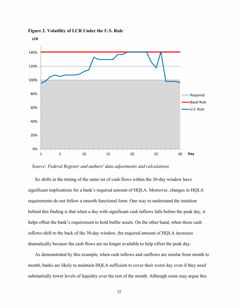
As shown in Figure 2, the LCR for this hypothetical bank varies considerably over the 30-
day window. Most of the time, the LCR is above the 100 percent minimum required. It even
equals the LCR computed under the Basel rule for 6 of the 30 days. Note that the LCR computed
under the Basel rule remains steady at just over 140 percent and never requires the bank to report
a shortfall. In contrast, under the U.S. rule, the bank must report an LCR deficiency for 6 of the
30 days. Moreover, for the 4-day consecutive deficiency at the end of the 30-day window, the
bank is also required to provide its supervisor a plan for remediation of the liquidity shortfall.12
12 The U.S. rule requires banks to submit remediation plans for deficiencies over three consecutive business days.
25
Figure 2. Volatility of LCR Under the U.S. Rule
So shifts in the timing of the same set of cash flows within the 30-day window have
significant implications for a bank’s required amount of HQLA. Moreover, changes in HQLA
requirements do not follow a smooth functional form. One way to understand the intuition
behind this finding is that when a day with significant cash inflows falls before the peak day, it
helps offset the bank’s requirement to hold buffer assets. On the other hand, when those cash
inflows shift to the back of the 30-day window, the required amount of HQLA increases
dramatically because the cash flows are no longer available to help offset the peak day.
As demonstrated by this example, when cash inflows and outflows are similar from month to
month, banks are likely to maintain HQLA sufficient to cover their worst day even if they need
substantially lower levels of liquidity over the rest of the month. Although some may argue this
0%
20%
40%
60%
80%
100%
120%
140%
1 5 10 15 20 25 30
LCR
Day
Required
Basel Rule
U.S. Rule
Source: Federal Register and authors' data adjustments and calculations
26
contributes to bank safety and soundness, the introduction of volatility into banks’ LCR
denominators makes comparisons across banks and over time far less meaningful in practice.
Analysts will need to decompose LCRs calculated under the U.S. rule into Basel-equivalent and
add-on components for comparison with LCRs computed under Basel standards.
Conclusion
Under both Basel and U.S. standards, covered banks’ LCRs can vary in complex, nonlinear
ways not necessarily related to underlying liquidity risk. This is, in part, due to the use of
min/max functions in the numerator and denominator. However, it is also because the metric was
built using a ratio approach, creating the potential for secured lending and borrowing transactions
to simultaneously affect the LCR numerator and denominator. A complementary gap approach
could be used to enhance the regulatory goal of a quantifiable measure of liquidity risk with
meaningful variance. For example, HQLA – net cash outflows > 0 could be an equivalent
regulatory standard.13 For peer analysis, this gap measure could be normalized by dividing it by
total assets or exposures. Such a change could help strengthen the LCR’s efficacy as a regulatory
metric. Alternatively, although the LCR is a stress metric, liquidity stress testing could be used
to address some of the shortcomings we identify in this paper.
Comparability of LCRs across banks is also reduced by substantial differences between the
Basel and U.S. rules for calculating the ratio. U.S. regulators made a change in implementing the
Basel standard to make it harder for banks to circumvent the HQLA diversification requirements
through their use of reverse repos. U.S. regulators also made changes to the Basel standard to
quantify liquidity mismatches within the 30-day window. However, there are potential
13 This would exclude the add-on term in the U.S. rule, and thus, would not capture liquidity mismatches within the 30-day window.

27
unintended consequences from those changes, including difficulty in interpreting daily
fluctuations in U.S. banks’ LCRs due to the maximum peak day add-on. Additionally, we
document examples in which a bank could appear comfortably above the standard using the
Basel approach, but could be significantly noncompliant under the U.S. rule. Finally, banks can
alter their LCRs through their use of repos and reverse repos under both the Basel and U.S.
standards.
Because of potential negative signaling effects, banks are likely to feel pressured to maintain
LCRs above 100 percent even during times of stress. Indeed, the Basel Committee recognizes the
threat to financial stability posed by banks attempting to maintain an LCR over 100 percent
during times of stress. In the January 2013 publication “Basel III: The Liquidity Coverage Ratio
and Liquidity Risk Monitoring Tools,” the committee notes, “The potential for contagion to the
financial system and additional restricted flow of credit or reduced market liquidity due to
actions to maintain an LCR of 100 (percent).” The committee also suggests that a bank
“periodically monetize a representative proportion of the assets in the stock [of HQLA] through
repo or outright sale, in order to test its access to the market, the effectiveness of its processes for
monetization, the availability of the assets, and to minimize the risk of negative signaling during
a period of actual stress.”
The literature also shows the LCR could have unintended negative effects on interbank
funding and interest rates through interactions with monetary policy. Banks’ secured funding
transactions with the central bank could alter their LCRs and potentially complicate the
implementation of monetary policy. Schmitz (2013) has already identified one likely regulatory
arbitrage strategy pursued by banks, namely obtaining HQLA from repos with the European
Central Bank by swapping non-HQLA for central bank reserves, which are Level 1 HQLA. In

28
light of the impacts of secured funding transactions on banks’ LCRs we have illustrated in this
paper, the LCR’s implications for central banks’ open market operations remain an important
area for further study.

29
References
Balasubramanyan, Lakshmi, and VanHoose, David D. “Bank Balance Sheet Dynamics Under a Regulatory Liquidity-coverage-ratio Constraint.” Journal of Macroeconomics 37 (2013): 53-67. Banerjee, Ryan N., and Mio, Hitoshi. “The Impact of Liquidity Regulation on Banks.” BIS Working Paper no. 470, Basel: Bank for International Settlements, 2014. Basel Committee on Banking Supervision. Basel III: The Liquidity Coverage Ratio and Liquidity Risk Monitoring Tools. Consultative Document. Bank for International Settlements, Basel: BCBS, January 2013.
Bech, Morten L., and Keister, Todd. “Liquidity Regulation and the Implementation of Monetary Policy. BIS Working Paper no. 432, Basel: Bank for International Settlements, 2013.
Bonner, Clemens, and Eijffinger, Sylvester. “The Impact of Liquidity Regulation on Financial Intermediation.” CEPR Discussion Paper no. 9124, London: Center for Economic Policy Research, 2013.
Griffin, Paul A. “Sensitive Foreign Payment Disclosures: the Security Market Impact.” Report of the Advisory Committee on Corporate Disclosure to the Securities and Exchange Commission, Washington: U.S. Government Printing Office, 1977, 693-743. Grossman, Sanford J. “The Informational Role of Warranties and Private Disclosure About Product Quality.” Journal of Law and Economics 24, no. 3 (1981): 461-483. Hartlage, Andrew W. “The Basel III Liquidity Coverage Ratio and Financial Stability.” Michigan Law Review 111, no. 3 (2012): 453-483. Hong, Han, Huang, Jing-Zhi and Wu, Deming. “The Information Content of Basel III Liquidity Risk Measure.” Journal of Financial Stability 15 (2014): 91-111. JPMorgan Chase. 2014 Annual Report. New York: JPMorgan Chase, April 8, 2015. Milgrom, Paul R. “Good News and Bad News: Representation Theorems and Applications.” Bell Journal of Economics 12, no. 2 (1981): 380-391.
Office of the Comptroller of the Currency, Board of Governors of the Federal Reserve System, and Federal Deposit Insurance Corporation. Liquidity Coverage Ratio: Liquidity Risk Measurement Standards. Final Rule, Federal Register 79, no. 197, October 10, Washington: OCC and others, 2014, 61440-61541.
Office of Financial Research. 2014 Annual Report. Washington: OFR, 2014. Ross, Stephen A. “The Economics of Information and the Disclosure Regulation Debate.” Issues in Financial Regulation. New York: McGraw-Hill (1979): 177-202.

30
Schmitz, Stefan W. “The Impact of the Liquidity Coverage Ratio (LCR) on the Implementation of Monetary Policy.” Economic Notes 42, no. 2 (2013): 135-170. Song, Guoxiang. “The Pro-cyclical Effects of Accounting Rules on Basel III Liquidity Regulation.” SSRN Working Paper: Social Science Research Network, December 2014. http://ssrn.com/abstract=2175689 (accessed June 5, 2015). van den End, Jan Willem, and Mark Kruidhof. “Modelling the Liquidity Ratio as Macroprudential Instrument.” Journal of Banking Regulation 14, no. 2 (2013): 91-106.