1

Measuring and Understanding Throughputof Network Topologies

Sangeetha Abdu Jyothi∗, Ankit Singla†, P. Brighten Godfrey∗, Alexandra Kolla∗∗University of Illinois at Urbana–Champaign †ETH Zurich

Abstract—High throughput is of particular interest in datacenter and HPC networks. Although myriad network topologieshave been proposed, a broad head-to-head comparison acrosstopologies and across traffic patterns is absent, and the rightway to compare worst-case throughput performance is a subtleproblem.

In this paper, we develop a framework to benchmark thethroughput of network topologies, using a two-pronged approach.First, we study performance on a variety of synthetic andexperimentally-measured traffic matrices (TMs). Second, weshow how to measure worst-case throughput by generating anear-worst-case TM for any given topology. We apply the frame-work to study the performance of these TMs in a wide rangeof network topologies, revealing insights into the performance oftopologies with scaling, robustness of performance across TMs,and the effect of scattered workload placement. Our evaluationcode is freely available.

I. INTRODUCTION

Throughput is a fundamental property of communicationnetworks: at what rate can data be carried across the networkbetween desired end-points? Particularly for data centers andhigh performance computing, an increase in throughput de-mand among compute elements has reinvigorated research onnetwork topology, and a large number of network topologieshave been proposed in the past few years to achieve highcapacity at low cost [3], [8], [9], [11], [14]–[16], [30], [38],[39], [43], [44].

However, there is little order to this large and ever-growingset of network topologies. We lack a broad comparison oftopologies, and there is no open, public framework availablefor testing and comparing topology designs. The absence ofa well-specified benchmark complicates research on networkdesign, making it difficult to evaluate a new design against thenumerous past proposals, and difficult for industry to knowwhich threads of research are most promising to adopt.

Our goal is to build a framework for accurate and consistentmeasurement of the throughput of network topologies, and usethis framework to benchmark proposed data center and HPCtopologies.

To accomplish this, we need metrics for comparison ofthroughput, and this turns out to be a subtle problem. Through-put can be measured by testing particular workloads, or trafficmatrices (TMs), but the immediate question is what TMs totest. One approach is to test a variety of common TMs, whichcan provide insight into the effect of topological structure forparticular use cases reflected by those specific TMs. However,

we argue it is useful to go beyond this. In HPC and datacenter networks, TMs may vary widely depending on theuse-case and across time as applications spin up and downor migrate [14], [18]–[21]. Although some applications mapwell onto certain topologies and known worst-case trafficpatterns [33], [42] can be avoided in such cases, a mixof multiple applications could still produce an unintendeddifficult TM. In fact, [19] observes that network contentionamong applications sharing an HPC system will worsen in thenear future (even after accounting for the expected increase innetwork speeds) as HPC applications grow in size and variety.Hence, it is useful to understand the worst-case performanceof a topology, for any TM. However, currently, there does notexist a systematic way to evaluate the worst-case throughputachievable in a network and to identify the traffic patternresponsible for it.

Our key contributions, then, are to (1) develop a heuristic tomeasure worst-case throughput, and (2) provide an expansivebenchmarking of a variety of topologies using a variety of TMs– TMs generated from real-world measurements, syntheticTMs, and finally our new near-worst-case TMs. We discusseach of these in more detail.

(1a) We evaluate whether cut-based metrics, such asbisection bandwidth and sparsest cut, solve the problemof estimating worst-case throughput. A number of studies(e.g. [2], [8], [40], [41], [45]) employ cut metrics. It has beennoted [46] that bisection bandwidth does not always predictaverage-case throughput (in a limited setting; §V). But do cutsmeasure worst-case throughput? We show that it does not,by proving the existence of two families of networks, A andB, where A has a higher cut-metric even though B supportsasymptotically higher worst-case throughput. Further, we showthat the mismatch between cuts and worst-case throughputexists even for highly-structured networks of small size – a 5-ary 3-stage butterfly with only 25 nodes – where the sparsest-cut found through brute force computation is strictly greaterthan the worst-case throughput.

(1b) Since cut metrics don’t achieve our goal, we develop aheuristic to measure worst-case throughput. We propose anefficient algorithm to generate a near-worst-case TM for anygiven topology. We show empirically that these near-worst-case TMs approach a theoretical lower bound of throughput inpractice. Note that Kodialam et. al. [25] previously developeda TM for a somewhat different reason1 which could be re-

1Upper-bounding throughput performance of a routing scheme using an LPformulation. In addition, [25] did not use their TM to benchmark topologies.SC16; Salt Lake City, Utah, USA; November 2016

978-1-4673-8815-3/16/$31.00 c©2016 IEEE

2

purposed as a near-worst-case TM. Compared with [25], ourmethodology finds TMs that are just as close to the worstcase, can be computed approximately 6× faster, and scales tonetworks 8× larger with the same memory limit.

(2) We perform a head-to-head benchmark of a widerange of topologies across a variety of workloads. Specifi-cally, we evaluate a set of 10 topologies proposed for datacenters and high performance computing, with our near-worst-case TMs, a selection of synthetic TMs, and real TMsmeasured from two operational Facebook data centers. Keyfindings of this study include:

• Which topologies perform well? We find the answerdepends on scale. At small scale, several topologies, partic-ularly DCell, provide excellent performance across nearlyall TMs. However, at ≥ 1000s of servers, proposals basedon expander graphs (Jellyfish, Long Hop, Slim Fly) providethe best performance, with the advantage increasing withscale (an observation confirmed by a recent data centerproposal [43]).These results add new information compared with past work.We find the three expanders have nearly identical perfor-mance for uniform traffic (e.g. all-to-all); this differs fromconclusions of [4], [41] which analyzed bisection bandwidthrather than throughput. We find that expanders significantlyoutperform fat trees; this differs from the results of [47]which concluded that fat trees perform as well or better. Wereplicate the result of [47] and show the discrepancy resultsfrom an inaccurate calculation of throughput and unequaltopology sizes.

• What topologies have robustly high performance evenwith worst-case traffic? The effect of near-worst-casetraffic differs. We find that certain topologies (Dragonfly,BCube) are less robust, dropping more substantially inperformance. Jellyfish and Long Hop are most robust.While fat trees are otherwise generally robust, we show thatunder a TM with a small fraction of large flows in thenetwork, fat trees perform poorly. We find this is due tolack of path diversity near the endpoints.

• How do real-world workloads perform? We experimentwith real world TMs from two different clusters basedon data from Facebook [34]. Surprisingly, in one verynonuniform TM we find that randomizing rack-level work-load placement consistently improves performance for allnetworks we tested other than fat trees and the expanders.The fact that expanders and fat trees perform well evenwithout this workload rearrangement is consistent with ourfinding that they are robust to worst-case performance. Butalso, for the other topologies, it indicates an intriguingopportunity for improving performance through better work-load placement.

To the best of our knowledge, this work is the mostexpansive comparison of network topology throughput to date,and the only one to use accurate and consistent methods. Ourresults provide insights that are useful in topology selectionand workload placement. But just as importantly, our evalu-ation framework and the set of topologies tested are freelyavailable [1]. We hope our tools will facilitate future work on

rigorously designing and evaluating networks, and replicationof research results.

II. METRICS FOR THROUGHPUT

In this section, we define throughput precisely. We thenstudy how to evaluate worst-case throughput: we consider cut-metrics, before presenting a heuristic algorithm that producesa near-worst-case traffic matrix.

A. Throughput defined

Our focus in this paper is on network throughput. Further-more, our focus is on network topology, not on higher-leveldesign like routing and congestion control.2 Therefore, themetric of interest is end-to-end throughput supported by anetwork in a fluid-flow model with optimal routing. We nextdefine this more precisely.

A network is a graph G = (V,E) with capacities c(u, v)for every edge (u, v) ∈ EG. Among the nodes V are servers,which send and receive traffic flows, connected through non-terminal nodes called switches. Each server is connected toone switch, and each switch is connected to zero or moreservers, and other switches. Unless otherwise specified, forswitch-to-switch edges (u, v), we set c(u, v) = 1, while server-to-switch links have infinite capacity. This allows us to stress-test the network topology itself, rather than the servers.

A traffic matrix (TM) T defines the traffic demand: forany two servers v and w, T (v, w) is an amount of requestedflow from v to w. We assume without loss of generality thatthe traffic matrix is normalized so that it conforms to the“hose model”: each server sends at most 1 unit of traffic andreceives at most 1 unit of traffic (∀v,

∑w T (v, w) ≤ 1 and∑

w T (w, v) ≤ 1).The throughput of a network G with TM T is the max-

imum value t for which T · t is feasible in G. That is,we seek the maximum t for which there exists a feasiblemulticommodity flow that routes flow T (v, w) · t throughthe network from each v to each w, subject to the linkcapacity and the flow conservation constraints. This can beformulated in a standard way as a linear program (omittedfor brevity) and is thus computable in polynomial time. If thenonzero traffic demands T (v, w) are equal, this is equivalentto the maximum concurrent flow [35] problem: maximizingthe minimum throughput of any requested end-to-end flow.

Note that we could alternately maximize the total through-put of all flows. We avoid this because it would allow thenetwork to pick and choose among the TM’s flows, givinghigh bandwidth only to the “easy” ones (e.g., short flows thatdo not cross a bottleneck). The formulation above ensures thatall flows in the given TM can be satisfied at the desired ratesspecified by the TM, all scaled by a constant factor.

We now have a precise definition of throughput, but itdepends on the choice of TM. How can we evaluate a

2There are many performance measures for networks that are not consideredhere, and higher-layer systems obviously affect throughput experienced by ap-plications. But our goal is a comprehensive understanding of the fundamentalgoal of high-throughput network topology. At this stage, systems-level issueswould be a distraction.

3

hypercube

Th

rou

ghpu

t

Sparsest Cut

cut > O(log n) * throughput (Impossible)

Graph A expanders

Graph B

Throughput > cut

(Impossible)

thro

ughput=

cut

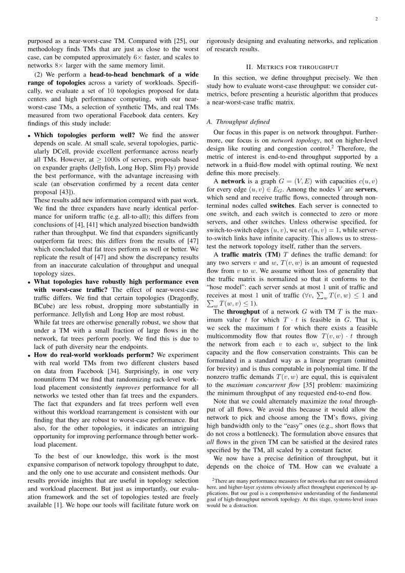
Fig. 1. Sparsest cut vs. Throughput

topology independent of assumptions about the traffic, if weare interested in worst-case traffic?

B. Cuts: a weak substitute for worst-case throughput

Cuts are generally used as proxies to estimate throughput.Since any cut in the graph upper-bounds the flow across thecut, if we find the minimum cut, we can bound the worst-caseperformance. Two commonly used cut metrics are:

(a) Bisection bandwidth: It is a widely used to providean evaluation of a topology’s performance independent of aspecific TM. It is the capacity of the worst-case cut that dividesthe network into two equal halves ( [31], p. 974).

(b) Sparsest cut: The sparsity of a cut is the ratio of itscapacity to the net weight of flows that traverse the cut, wherethe flows depend on a particular TM. Sparsest cut refers to theminimum sparsity in the network. The special case of uniformsparsest cut assumes the all-to-all TM.

Cuts provide an upper-bound on worst-case network perfor-mance, are simple to state, and can sometimes be calculatedwith a formula. However, they have several limitations.

(1) Sparsest cut and bisection bandwidth are not actuallyTM-independent, contrary to the original goal of evaluatinga topology independent of traffic. Bisection bandwidth andthe uniform sparsest cut correspond to the worst cuts forthe complete (all-to-all) TM, so they have a hidden implicitassumption of this particular TM.

(2) Even for a specific TM, computing cuts is NP-hard,and it is believed that there is no efficient constant factorapproximation algorithm [6], [13]. In contrast, throughput iscomputable in polynomial time for any specified TM.

(3) Cuts are only a loose upper-bound for worst-casethroughput. This may be counter-intuitive if our intuition isguided by the well-known max-flow min-cut theorem whichstates that in a network with a single flow, the maximumachievable flow is equal to the minimum capacity over all cutsseparating the source and the destination [10], [12]. However,this no longer holds when there are more than two flows inthe network, i.e., multi-commodity flow: the maximum flow(throughput) can be an O(log n) factor lower than the sparsestcut [28]. Hence, cuts do not directly capture the maximumflow.

Figure 1 depicts this relationship between cuts and through-put. Here we focus on sparsest cut.3 The flow (throughput) inthe network cannot exceed the upper bound imposed by theworst-case cut. On the other hand, the cut cannot be more thana factor O(log n) greater than the flow [28]. Thus, any graphand an associated TM can be represented by a unique pointin the region bounded by these limits.

While this distinction is well-established [28], we strengthenthe point by showing that it can lead to incorrect decisionswhen evaluating networks. Specifically, we will exhibit a pairof graphs A and B such that, as shown in Figure 1, A hashigher throughput but B has higher sparsest cut. If sparsestcut is the metric used to choose a network, graph B will bewrongly assessed to have better performance than graph A,while in fact it has a factor Ω(

√log n) worse performance!

Graph A is a clustered random graph adapted from previouswork [37] with n nodes and degree 2d. A is composed oftwo equal-sized clusters with n/2 nodes each. Each node in acluster is connected by degree α to nodes inside its cluster, anddegree β to nodes in the other cluster, such that α+β = 2d. Ais sampled uniformly at random from the space of all graphssatisfying these constraints. We can pick α and β such thatβ = Θ( α

logn ). Then, as per [37] (Lemma 3), the throughputof A (denoted TA) and its sparsest cut (denoted ΦA) are bothΘ( 1

n logn ).Let graph G be any 2d-regular expander on N = n

dp nodes,where d is a constant and p is a parameter we shall adjustlater. Graph B is constructed by replacing each edge of Gwith a path of length p. It is easy to see that B has n nodes.We prove in the tech report [22], the following theorem.

Theorem 1. TB = O( 1nplogn ) and ΦB = Ω( 1

np ).

In the above, setting p = 1 corresponds to the ‘expanders’point in Figure 1: both A and B have the same throughput(within constant factors), but the B’s cut is larger by O(log n).Increasing p creates an asymptotic separation in both the cutand the throughput such that ΦA < ΦB , while TA > TB .

Intuition. The reason that throughput may be smaller thansparsest cut is that in addition to being limited by bottlenecks,the network is limited by the total volume of “work” it hasto accomplish within its total link capacity. That is, if the TMhas equal-weight flows,

Throughput per flow ≤ Total link capacity

# of flows · Avg path lengthwhere the total capacity is

∑(i,j)∈E c(i, j) and the average

path length is computed over the flows in the TM. This“volumetric” upper bound may be tighter than a cut-basedbound.

Based on the above result and experimental confirmation in§III, we conclude that cuts are not a good choice to evaluatethroughput. Cuts still capture important topological propertiessuch as the difficulty of partitioning a network, and physicallayout (packaging and cabling) complexity. However, theseproperties are outside the scope of our study of throughput.

3We pick one for simplicity, and sparsest cut has an advantage in robustness.Bisection bandwidth is forced to cut the network in equal halves, so it canmiss more constrained bottlenecks that cut a smaller fraction of the network.

4

0

0.2

0.4

0.6

0.8

1

3 4 5 6 7 8 9

Abs

olut

e T

hrou

ghpu

t

Hypercube degree

All to AllRandom Matching - 10Random Matching - 2Random Matching - 1

Kodialam TMLongest Matching

Lower bound

0

0.2

0.4

0.6

0.8

1

3 4 5 6 7 8 9

Random Graph degree

All to AllRandom Matching - 10Random Matching - 2Random Matching - 1

Kodialam TMLongest Matching

Lower bound

0

0.2

0.4

0.6

0.8

1

1.2

4 5 6 7 8 9 10 11 12

Fat tree degree

All-to-allRandom Matching

Kodialam TMLongest Matching

Lower bound

Fig. 2. Throughput resulting from several different traffic matrices in three topologies

C. Towards a worst-case throughput metric

Having exhausted cut-based metrics, we return to the orig-inal metric of throughput defined in §II-A. We can evaluatenetwork topologies directly in terms of throughput (via LPoptimization software) for specific TMs. The key, of course,is how to choose the TM. Our evaluation can include a varietyof synthetic and real-world TMs, but as discussed in theintroduction, we also want to evaluate topologies’ robustnessto unexpected TMs.

If we can find a worst-case TM, this would fulfill ourgoal. However, computing a worst-case TM is an unsolved,computationally non-trivial problem [7].4 Here, we offer anefficient heuristic to find a near-worst-case TM which can beused to benchmark topologies.

We begin with the complete or all-to-all TM TA2A whichfor all v, w has TA2A(v, w) = 1

n . We observe that TA2A iswithin 2× of the worst case TM. This fact is simple and knownto some researchers, but at the same time, we have not seenit in the literature, so we give the statement here and proof ina tech report [22].

Theorem 2. Let G be any graph. If TA2A is feasible in G withthroughput t, then any hose model traffic matrix is feasible inG with throughput ≥ t/2.

Can we get closer to the worst case TM? In our experience,TMs with a smaller number of “elephant” flows are moredifficult to route than TMs with a large number of small flows,like TA2A. This suggests a random matching TM in whichwe have only one outgoing flow and one incoming flow perserver, chosen uniform-randomly among servers.

Can we get even closer to the worst-case TM? Intuitively,the all-to-all and random matching TMs will tend to findsparse cuts, but only have average-length paths. Drawing onthe intuition that throughput decreases with average flow pathlength, we seek to produce traffic matrices that force the useof long paths. To do this, given a network G, we computeall-pairs shortest paths and create a complete bipartite graphH , whose nodes represent all sources and destinations in G,and for which the weight of edge v → w is the length ofthe shortest v → w path in G. We then find the maximumweight matching in H . The resulting matching corresponds

4Our problem corresponds to the separation problem of the minimum-costrobust network design in [7]. This problem is shown to be hard for the single-source hose model. However, the complexity is unknown for the hose modelwith multiple sources which is the scenario we consider.

to the pairing of servers which maximizes average flow pathlength, assuming flow is routed on shortest paths between eachpair. We call this a longest matching TM, and it will serveas our heuristic for a near-worst-case traffic.

Kodialam et al. [25] proposed another heuristic to find anear-worst-case TM: maximizing the average path length of aflow. This Kodialam TM is similar to the longest matching butmay have many flows attached to each source and destination.This TM was used in [25] to evaluate oblivious routingalgorithms, but there was no evaluation of how close it isto the worst case, so our evaluation here is new.

Figure 2 shows the resulting throughput of these TMs inthree topologies: hypercubes, random regular graphs, and fattrees [3]. In all cases, A2A traffic has the highest throughput;throughput decreases or does not change as we move toa random matching TM with 10 servers per switch, andprogressively decreases as the number of servers per switchis decreased to 1 under random matching, and finally to theKodialam TM and the longest matching TM. We also plotthe lower bound given by Theorem 2: TA2A/2. Comparisonacross topologies is not relevant here since the topologies arenot built with the same “equipment” (node degree, number ofservers, etc.)

We chose these three topologies to illustrate cases whenour approach is most helpful, somewhat helpful, and leasthelpful at finding near-worst-case TMs. In the hypercube,the longest matching TM is extremely close to the worst-case performance. To see why, note that the longest pathshave length d in a d-dimensional hypercube, twice as longas the mean path length; and the hypercube has n · d uni-directional links. The total flow in the network will thus be(#flows ·average flow path length) = n ·d. Thus, all linkswill be perfectly utilized if the flow can be routed, whichempirically it is. In the random graph, there is less variationin end-to-end path length, but across our experiments thelongest matching is always within 1.5× of the provable lowerbound (and may be even closer to the true lower bound, sinceTheorem 2 may not be tight). In the fat tree, which is herebuilt as a three-level nonblocking topology, there is essentiallyno variation in path length since asymptotically nearly all pathsgo three hops up to the core switches and three hops downto the destination. Here, our TMs are no worse than all-to-all,and the simple TA2A/2 lower bound is off by a factor of 2from the true worst case (which is throughput of 1 as this isa nonblocking topology).

5

The longest matching and Kodialam TMs are identical inhypercubes and fat trees. On random graphs, they yield slightlydifferent TMs, with longest matching yielding marginallybetter results at larger sizes. In addition, longest matchinghas a significant practical advantage: it produces far fewerend-to-end flows than the Kodialam TM. Since the memoryrequirements of computing throughput of a given TM (via themulticommodity flow LP) depends on the number of flows,longest matching requires less memory and compute time.For example, in random graphs on a 32 GB machine usingthe Gurobi optimization package, the Kodialam TM can becomputed up to 128 nodes while the longest matching scalesto 1,024, while being computed roughly 6× faster. Hence, wechoose longest matching as our representative near-worst-casetraffic matrix.

D. Summary and implications

Directly evaluating throughput with particular TMs usingLP optimization is both more accurate and more tractable thancut-based metrics. In choosing a TM to evaluate, both “averagecase” and near-worst-case TMs are reasonable choices. Ourevaluation will employ multiple synthetic TMs and mea-surements from real-world applications. For near-worst-casetraffic, we developed a practical heuristic, the longest matchingTM, that often succeeds in substantially worsening the TMcompared with A2A.

Note that measuring throughput directly (rather than viacuts) is not in itself a novel idea: numerous papers haveevaluated particular topologies on particular TMs. Our con-tribution is to provide a rigorous analysis of why cuts do notalways predict throughput; a way to generate a near-worst-caseTM for any given topology; and an experimental evaluationbenchmarking a large number of proposed topologies on avariety of TMs.

III. EXPERIMENTAL METHODS

In this section, we present our experimental methodologyand detailed analysis of our framework. We attempt to answerthe following questions: Are cut-metrics indeed worse pre-dictors of performance? When measuring throughput directly,how close do we come to worst-case traffic?

A. Methodology

Before delving into the experiments, we explain the methodsused for computing throughput. We also elaborate on the trafficworkloads and topologies used in the experiments.

1) Computing throughput: Throughput is computed as asolution to a linear program whose objective is to maximizethe minimum flow across all flow demands, as explained in§II. We use the Gurobi [17] linear program solver. Throughputdepends on the traffic workload provided to the network.

2) Traffic workload: We evaluate two main categories ofworkloads: (a) real-world measured TMs from Facebook clus-ters and (b) synthetic TMs, which can be uniform weight ornon-uniform weight. Synthetic workloads belong to three mainfamilies: all-to-all, random matching and longest matching

(near-worst-case). In addition, we need to specify where thetraffic endpoints (sources and destinations, i.e., servers) areattached. In structured networks with restrictions on server-locations (fat-tree, BCube, DCell), servers are added at thelocations prescribed by the models. For example, in fat-trees,servers are attached only to the lowest layer. For all othernetworks, we add servers to each switch. Note that our trafficmatrices effectively encode switch-to-switch traffic, so theparticular number of servers doesn’t matter.

3) Topologies: Our evaluation uses 10 families of com-puter networks. Topology families evaluated are: BCube [15],DCell [16], Dragonfly [24], Fat Tree [29], Flattened butter-fly [23], Hypercubes [5], HyperX [2], Jellyfish [38], LongHop [41] and Slim Fly [4]. For evaluating the cut-basedmetrics in a wider variety of environments, we consider 66non-computer networks – food webs, social networks, andmore [1].

B. Do cuts predict worst-case throughput?

In this section, we experimentally evaluate whether cut-based metrics predict throughput. We generate multiple net-works from each of our topology families (with varyingparameters such as size and node degree), compute throughputwith the longest matching TM, and find sparse cuts usingheuristics with the same longest matching TM. We show that:• In several networks, bisection bandwidth cannot predict

throughput accurately. For a majority of large networks,our best estimate of sparsest-cut differs from the computedworst-case throughput by a large factor.

• Even in a well-structured network of small size (where bruteforce is feasible), sparsest-cut can be higher than worst-casethroughput.Since brute-force computation of cuts is possible only

on small networks (up to 20 nodes), we evaluate bisectionbandwidth and sparsest cut on networks of feasible size (115networks total – 100 Jellyfish networks and 15 networksfrom 7 families of topologies). Of the 8 topology familiestested, we found that bisection bandwidth accurately predictedthroughput in only 5 of the families while sparsest cut gives thecorrect value in 7. The average error (difference between cutand throughput) is 7.6% for bisection bandwidth and 6.2% forsparsest cut (in networks where they differ from throughput).Maximum error observed was 56.3% for bisection bandwidthand 6.2% for sparsest cut.

Although sparsest cut does a better job at estimatingthroughput at smaller sizes, we have found that in a 5-ary3-stage flattened butterfly with only 25 switches and 125servers, the throughput is less than the sparsest cut (and thebisection bandwidth). Specifically, the absolute throughput inthe network is 0.565 whereas the sparsest-cut is 0.6. Thisshows that even in small networks, throughput can be differentfrom the worst-case cut. While the differences are not large inthe small networks where brute force computation is feasible,note that since cuts and flows are separated by an Θ(log n)factor, we should expect them to grow.

Sparsest cut being the more accurate cut metric, we extendthe sparsest cut estimation to larger networks. Here we have

6

0

5

10

15

20

0 5 10 15 20

Thro

ughput

Sparsest Cut

BCubeDCell

DragonflyFat Tree

Flattened BFHypercube

HyperXJellyfish

Long HopSlim Fly

Natural networks

(a) Throughput vs. cut for all graphs

0

1

2

3

4

5

0 1 2 3 4 5

Thro

ug

hp

ut

Sparsest Cut

(b) Throughput vs. cut for selectedgraphs (zoomed version of (a))

Fig. 3. Throughput vs. cut. (Comparison is valid for individual networks, not across networks, since they have different numbers of nodesand degree distributions.)

1

1.2

1.4

1.6

1.8

2

BCubeDCell

DragonFlyFatTree

FlattenedBF

HypercubeHyperX

Jellyfish

LongHopSlimFly

Thro

ug

hp

ut

Topology

A2A RM(5) RM(1) LM

Fig. 4. Comparison of throughput under different traffic matricesnormalized with respect to theoretical lower bound

to use heuristics to compute sparsest cut, but we computeall of an extensive set of heuristics (limited brute-force,selective brute-force involving one or two nodes in a subset,eigenvector-based optimization, etc.) and use the term sparsecut to refer to the sparsest cut that was found by any of theheuristics. Sparse cuts differ from throughput substantially,with up to a 3× discrepancy as shown in Figure 3. In onlya small number of cases, the cut equals throughput. Thedifference between cut and throughput is pronounced. Forexample, Figure 3(b) shows that although HyperX networks ofdifferent sizes have approximately same flow value (y axis),they differ widely in sparsest cut (x axis). This shows thatestimation of worst-case throughput performance of networksusing cut-based metrics can lead to erroneous results.

C. Does longest matching approach the true worst case?

We compare representative samples from each family oftopology under four types of TM: all to all (A2A), randommatching with 5 servers per switch, random matching with1 server per switch, and longest matching. Figure 4 showsthe throughput values normalized so that the theoretical lowerbound on throughput is 1, and therefore A2A’s throughput is2. For all networks, TA2A ≥ TRM(5) ≥ TRM(1) ≥ TLM ≥ 1,i.e., all-to-all is consistently the easiest TM in this set, followedby random matchings, longest matching, and the theoreticallower bound. This confirms our intuition discussed in §II-C.

(As in Figure 3, throughput comparisons are valid across TMsfor a particular network, not across networks since the numberof links and servers varies across networks.)

Our longest matching TM is successful in matching thelower bound for BCube, Hypercube, HyperX, and (nearly)Dragonfly. In all other families except fat trees, the trafficunder longest matching is significantly closer to the lowerbound than with the other TMs. In fat trees, throughput underA2A and longest matching are equal. This is not a shortcomingof the metric, rather its the lower bound which is loose here:in fat trees, it can be easily verified that the flow out of eachtop-of-rack switch is the same under all symmetric TMs (i.e.,with equal-weight flows and the same number of flows intoand out of each top-of-rack switch).

In short, these results show that (1) the heuristic for near-worst-case traffic, the longest matching TM, is a significantlymore difficult TM than A2A and RM and often approaches thelower bound; and (2) throughput measurement using longestmatching is a more accurate estimate of worst-case throughputperformance than cut-based approximations, in addition tobeing substantially easier to compute.

IV. TOPOLOGY EVALUATION

In this section, we present the results of our topologyevaluation with synthetic and real-world workloads, and ournear-worst-case TM.

But first, there is one more piece of the puzzle to allowcomparison of networks. Networks may be built with differentequipment – with a wide variation in number of switchesand links. The raw throughput value does not account forthis difference in hardware resources, and most proposedtopologies can only be built with particular discrete numbersof servers, switches, and links, which inconveniently do notmatch.

Fortunately, uniform-random graphs as in [38] can be con-structed for any size and degree distribution. Hence, randomgraphs serve as a convenient benchmark for easy comparisonof network topologies. Our high-level approach to evaluating anetwork is to: (i) compute the network’s throughput; (ii) builda random graph with precisely the same equipment, i.e., thesame number of nodes each with the same number of links

7

0 0.2 0.4 0.6 0.8

1 1.2 1.4 1.6

100 1000 10000

Rel

. Thr

ough

put

Number of servers

BCubeDCell

Dragonfly

Fat treeFlattened BF

Hypercube

0 0.2 0.4 0.6 0.8

1 1.2 1.4 1.6

100 1000 10000

Rel

. Thr

ough

put

Number of servers

(a) All to All TM

0 0.2 0.4 0.6 0.8

1 1.2 1.4 1.6

100 1000 10000

Rel

. Thr

ough

put

Number of servers

(b) Random Matching TM

0 0.2 0.4 0.6 0.8

1 1.2 1.4 1.6

100 1000 10000

Rel

. Thr

ough

put

Number of servers

(c) Longest Matching TM

Fig. 5. Comparison of TMs on topologies

as the corresponding node in the original graph, (iii) computethe throughput of this same-equipment random graph underthe same TM; (iv) normalize the network’s throughput withthe random graph’s throughput for comparison against othernetworks. This normalized value is referred to as relativethroughput. Unless otherwise stated, each data-point is anaverage across 10 iterations, and all error bars are 95% two-sided confidence intervals. Minimal variations lead to narrowerror bars in networks of size greater than 100.

A. Synthetic Workloads

We evaluate the performance of 10 types of computernetworks under two categories of synthetic workloads: (a)uniform weight and (b) non-uniform weight.

1) Uniform-Weight Synthetic WorkloadsWe evaluate three traffic matrices with equal weight across

flows: all to all, random matching with one server, and longest

0 0.2 0.4 0.6 0.8

1 1.2 1.4 1.6

100 1000 10000

Rel

. Thr

ough

put

Number of servers

HyperXJellyfish

Long HopSlim Fly

0 0.2 0.4 0.6 0.8

1 1.2 1.4 1.6

100 1000 10000

Rel

. Thr

ough

put

Number of servers

(a) All to All TM

0 0.2 0.4 0.6 0.8

1 1.2 1.4 1.6

100 1000 10000R

el. T

hrou

ghpu

tNumber of servers

(b) Random Matching TM

0 0.2 0.4 0.6 0.8

1 1.2 1.4 1.6

100 1000 10000

Rel

. Thr

ough

put

Number of servers

(c) Longest Matching TM

Fig. 6. Comparison of TMs on more topologies

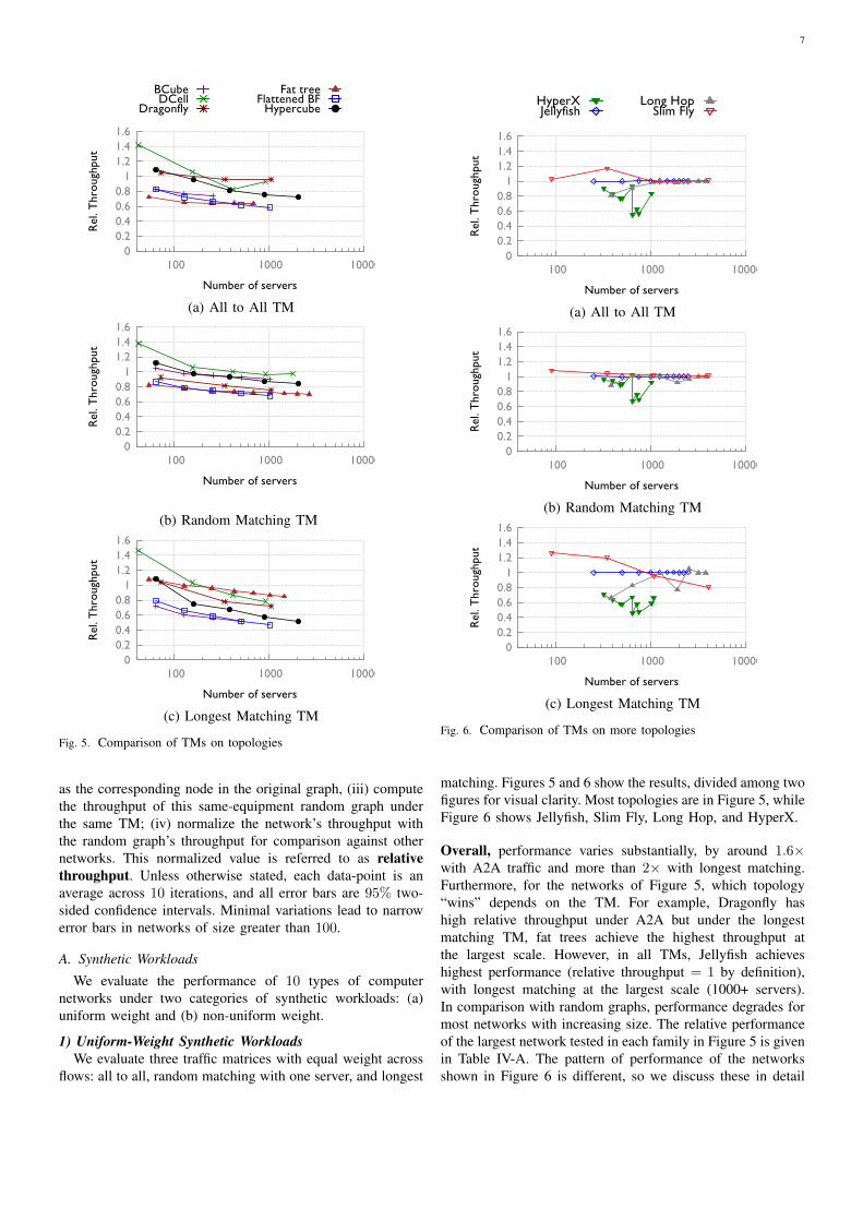
matching. Figures 5 and 6 show the results, divided among twofigures for visual clarity. Most topologies are in Figure 5, whileFigure 6 shows Jellyfish, Slim Fly, Long Hop, and HyperX.

Overall, performance varies substantially, by around 1.6×with A2A traffic and more than 2× with longest matching.Furthermore, for the networks of Figure 5, which topology“wins” depends on the TM. For example, Dragonfly hashigh relative throughput under A2A but under the longestmatching TM, fat trees achieve the highest throughput atthe largest scale. However, in all TMs, Jellyfish achieveshighest performance (relative throughput = 1 by definition),with longest matching at the largest scale (1000+ servers).In comparison with random graphs, performance degrades formost networks with increasing size. The relative performanceof the largest network tested in each family in Figure 5 is givenin Table IV-A. The pattern of performance of the networksshown in Figure 6 is different, so we discuss these in detail

8

next.

Topologyfamily

All-To-All

RandomMatching

Longestmatching

BCube (2-ary) 73% 90% 51%DCell (5-ary) 93% 97% 79%Dragonfly 95% 76% 72%Fat tree 65% 73% 89%Flattened BF(2-ary) 59% 71% 47%

Hypercube 72% 84% 51%TABLE I

RELATIVE THROUGHPUT AT THE LARGEST SIZE TESTED UNDERDIFFERENT TMS

HyperX [2] has irregular performance across scale. Thevariations arise from the choice of underlying topology: Givena switch radix, number of servers and desired bisectionbandwidth, HyperX attempts to find the least cost topologyconstructed from the building blocks – hypercube and flattenedbutterfly. Even a slight variation in one of the parameters canlead to a significant difference in HyperX construction andhence throughput.

We plot HyperX results for networks with bisection band-width of 0.4, i.e., in the worst case the network can supportflow from 40% of the hosts without congestion. In the worstcase, the HyperX network that can support 648 hosts achievesa relative throughput of 55% under all-to-all traffic. For thesame network, relative performance improves to 67% underrandom matching but further degrades to 45% under longestmatching. We investigate the performance of HyperX networkswith different bisection bandwidths under the longest matchingTM in Figure 7 and observe that the performance varieswidely with network size under all values of bisection. Moreimportantly, this further illustrates that high bisection does notguarantee high performance.

Jellyfish [38] is our benchmark, and its (average) relativeperformance is 100% under all workloads by definition. Per-formance depends on randomness in the construction, butat larger sizes, performance differences between Jellyfishinstances are minimal (≈ 1%).

Long Hop networks [41] In Figure 8, we show that therelative throughput of Long Hop networks approaches 1 atlarge sizes under the longest matching TM. Similar trendsare observed under all-to-all and random matching workloads.The paper [41] claimed high performance (in terms of bisec-tion bandwidth) with substantially less equipment than pastdesigns, but we find that while Long Hop networks do havehigh performance, they are no better than random graphs, andsometimes worse.

Slim Fly [4] It was noted in [4] that Slim Fly’s key advantageis path length. We observe in Figure 9 that the topologyindeed has extremely short paths – about 85-90% relativeto the random graph – but this does not translate to higherthroughput. Slim Fly’s performance is essentially identical torandom graphs under all-to-all and random matching TMswith a relative performance of 101% using both. Relativethroughput under the longest matching TM decreases with

scale, dropping to 80% at the largest size tested. Hence,throughput performance cannot be predicted solely based onthe average path length.

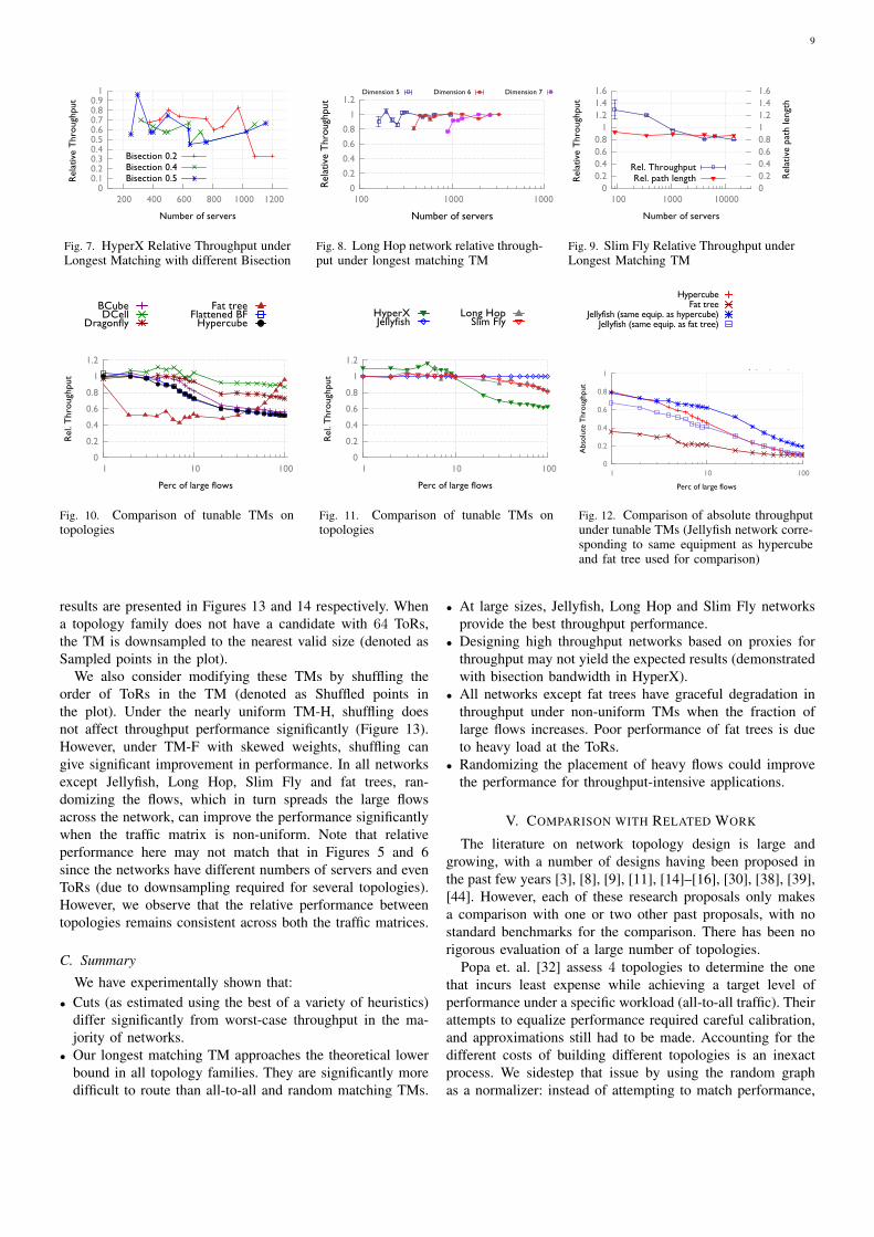
2) Non-Uniform Weight Synthetic WorkloadsIn order to understand the robustness of throughput perfor-

mance against variations in TM, we consider the response oftopologies to non-uniform traffic matrices. Using the longestmatching TM, we assign a weight of 10 to x% of flows inthe network which are chosen randomly while all other flowshave a weight of 1. Thus, we have a longest matching TMmodified so that a fraction of flows have higher demand thanthe rest. We vary x to understand the response of topologiesto skewed traffic matrices. The experiment is conducted on arepresentative sample from each topology class. Note that therelative throughput at 0% (which is not plotted) will be equalto that at 100% since all flows are scaled by the same factor.

We observe in Figures 10 and 11 that all topologies exceptfat trees perform well when there are a few large flows inthe network. To further understand the anomaly with fat trees,we look at the absolute throughput in fat tree, hypercube andJellyfish network built with matching gear in Figure 12. Trendsof other networks are similar to hypercube. The anomalousbehavior of fat trees arises due to the fact that load on linksconnected to the top-of-rack switch (ToR) in fat trees is fromthe directly connected servers only. In all other networks,under longest matching, links connected to ToRs carry trafficbelonging to flows that do not originate or terminate at theToR. Since the load is spread more evenly, a few large flowsdo not affect the overall throughput. Note that fat trees canbe built to be non-blocking, with high performance for anytraffic; what these results show is that for these TMs, fat treeswould pay a high price in equipment cost to achieve full non-blocking throughput, relative to other topology options.

Overall, we find that under traffic matrices with non-uniform demands, the Jellyfish, DCell, Long hop and SlimFly topologies perform better than other topologies. Whileall other topologies exhibit graceful degradation of throughputwith increase in the percentage of large flows, fat trees giveanomalous behavior due to the load on the ToRs.

B. Real-world workloads

Roy et al. [34] presents relative traffic demands measuredduring a period of 24 hours in two 64-rack clusters operatedby Facebook. The first TM corresponds to a Hadoop clusterand has nearly equal weights. The second TM from a frontendcluster is more non-uniform, with relatively heavy traffic at thecache servers and lighter traffic at the web servers. Since theraw data is not publicly available, we processed the paper’splot images to retrieve the approximate weights for inter-rack traffic demand with an accuracy of 10i in the interval[10i, 10i+1) (from data presented in color-coded log scale).Since our throughput computation rescales the TM anyway,relative weights are sufficient. Given the scale factor, thereal throughput can be obtained by multiplying the computedthroughput with the scale factor.

We test our slate of topologies with the Hadoop clusterTM (TM-H) and the frontend cluster TM (TM-F) and the

9

0 0.1 0.2 0.3 0.4 0.5 0.6 0.7 0.8 0.9

1

200 400 600 800 1000 1200

Rel

ativ

e T

hrou

ghpu

t

Number of servers

Bisection 0.2Bisection 0.4Bisection 0.5

Fig. 7. HyperX Relative Throughput underLongest Matching with different Bisection

0

0.2

0.4

0.6

0.8

1

1.2

100 1000 10000

Rel

ativ

e T

hrou

ghpu

t

Number of servers

Dimension 5 Dimension 6 Dimension 7

Fig. 8. Long Hop network relative through-put under longest matching TM

0 0.2 0.4 0.6 0.8

1 1.2 1.4 1.6

100 1000 10000 0 0.2 0.4 0.6 0.8 1 1.2 1.4 1.6

Rel

ativ

e T

hrou

ghpu

t

Rel

ativ

e pa

th le

ngth

Number of servers

Rel. ThroughputRel. path length

Fig. 9. Slim Fly Relative Throughput underLongest Matching TM

0 0.2 0.4 0.6 0.8

1 1.2 1.4 1.6

100 1000 10000

Rel

. Thr

ough

put

Number of servers

BCubeDCell

Dragonfly

Fat treeFlattened BF

Hypercube

0 0.2 0.4 0.6 0.8

1 1.2 1.4 1.6

100 1000 10000

Rel

. Thr

ough

put

Number of servers

HyperXJellyfish

Long HopSlim Fly

0

0.2

0.4

0.6

0.8

1

1 10 100

Abs

olut

e T

hrou

ghpu

t

Perc of large flows

HypercubeFat tree

Jellyfish (same equip. as hypercube)Jellyfish (same equip. as fat tree)

0

0.2

0.4

0.6

0.8

1

1.2

1 10 100

Rel

. Thr

ough

put

Perc of large flows

Fig. 10. Comparison of tunable TMs ontopologies

0

0.2

0.4

0.6

0.8

1

1.2

1 10 100

Rel

. Thr

ough

put

Perc of large flows

Fig. 11. Comparison of tunable TMs ontopologies

0

0.2

0.4

0.6

0.8

1

1 10 100

Abs

olut

e T

hrou

ghpu

t

Perc of large flows

HypercubeFat tree

Jellyfish (hypercube)Jellyfish (fat tree)

Fig. 12. Comparison of absolute throughputunder tunable TMs (Jellyfish network corre-sponding to same equipment as hypercubeand fat tree used for comparison)

results are presented in Figures 13 and 14 respectively. Whena topology family does not have a candidate with 64 ToRs,the TM is downsampled to the nearest valid size (denoted asSampled points in the plot).

We also consider modifying these TMs by shuffling theorder of ToRs in the TM (denoted as Shuffled points inthe plot). Under the nearly uniform TM-H, shuffling doesnot affect throughput performance significantly (Figure 13).However, under TM-F with skewed weights, shuffling cangive significant improvement in performance. In all networksexcept Jellyfish, Long Hop, Slim Fly and fat trees, ran-domizing the flows, which in turn spreads the large flowsacross the network, can improve the performance significantlywhen the traffic matrix is non-uniform. Note that relativeperformance here may not match that in Figures 5 and 6since the networks have different numbers of servers and evenToRs (due to downsampling required for several topologies).However, we observe that the relative performance betweentopologies remains consistent across both the traffic matrices.

C. Summary

We have experimentally shown that:• Cuts (as estimated using the best of a variety of heuristics)

differ significantly from worst-case throughput in the ma-jority of networks.

• Our longest matching TM approaches the theoretical lowerbound in all topology families. They are significantly moredifficult to route than all-to-all and random matching TMs.

• At large sizes, Jellyfish, Long Hop and Slim Fly networksprovide the best throughput performance.

• Designing high throughput networks based on proxies forthroughput may not yield the expected results (demonstratedwith bisection bandwidth in HyperX).

• All networks except fat trees have graceful degradation inthroughput under non-uniform TMs when the fraction oflarge flows increases. Poor performance of fat trees is dueto heavy load at the ToRs.

• Randomizing the placement of heavy flows could improvethe performance for throughput-intensive applications.

V. COMPARISON WITH RELATED WORK

The literature on network topology design is large andgrowing, with a number of designs having been proposed inthe past few years [3], [8], [9], [11], [14]–[16], [30], [38], [39],[44]. However, each of these research proposals only makesa comparison with one or two other past proposals, with nostandard benchmarks for the comparison. There has been norigorous evaluation of a large number of topologies.

Popa et. al. [32] assess 4 topologies to determine the onethat incurs least expense while achieving a target level ofperformance under a specific workload (all-to-all traffic). Theirattempts to equalize performance required careful calibration,and approximations still had to be made. Accounting for thedifferent costs of building different topologies is an inexactprocess. We sidestep that issue by using the random graphas a normalizer: instead of attempting to match performance,

10

0 0.2 0.4 0.6 0.8

1 1.2 1.4

BCubeDCell

DragonFly

FatTreeFlatte

nedBFHypercube

HyperXJellyfishLongHop

SlimFlyNor

mal

ized

Thr

ough

put

Topology

Sampled Shuffled

Fig. 13. Comparison of topologies with TM-H( [34])

0 0.2 0.4 0.6 0.8

1 1.2 1.4

BCubeDCell

DragonFly

FatTreeFlatte

nedBFHypercube

HyperXJellyfishLongHop

SlimFlyNor

mal

ized

Thr

ough

put

Topology

Sampled Shuffled

Fig. 14. Comparison of topologies with TM-F( [34])

0

0.2

0.4

0.6

0.8

1

1.2

Abs

olu

te T

hro

ughp

ut

Comparison 1:[Yuan]

Comparison 2:Opt. throughput

Comparison 3:Opt. throughput,same equipment

Fat tree Jellyfish

Fig. 15. Throughput comparison of Fat Treeand Jellyfish based on [47], showing theeffect of two methodological changes

for each topology, we build a random graph with identicalequipment, and then compare throughput performance of thetopology with that of the random graph. This alleviates theneed for equalizing configurations, thereby making it easy forothers to use our tools, and to test arbitrary workloads.

Yuan et al. [47] compared the performance of fat treesand Jellyfish with HPC traffic and a specific routing scheme,concluding they have similar performance, which disagreeswith our results. We replicated the method of [47] and wereable to reproduce their result of similar throughput using theA2A TM (Fig. 15, Comparison 1). Their method splits flowsinto sub-flows and routes them along certain paths accordingto a routing scheme called LLSKR. It then estimates eachsubflow’s throughput by counting and inverting the maximumnumber of intersecting subflows at a link along the path.Our LP-based exact throughput computation with the sameLLSKR path restrictions yields slightly higher throughput infat trees and substantially higher in Jellyfish, now 30% greaterthan fat trees (Fig. 15, Comparison 2). This is even thoughwe now maximize the minimum flow, while [47] measuredthe average. A second issue with the comparison in [47] isthat more servers are added to Jellyfish (160 servers) thanto fat tree (128 servers) with 80 switches in each topology.Equalizing all equipment, with 80 switches and 128 serversin both topologies, increases the performance gap to 65%(Comparison 3).

In a later work, Yuan et. al. [46] compared performance ofmultiple topologies. The throughput calculation was similarto [47] discussed above so it may differ from an exact LP-based method. In addition, [46] uses single-path routing. Aspointed out in [46], single-path routing can perform sig-nificantly differently than multipath. Moreover, in modernenterprise private cloud data centers as well as hyperscalepublic clouds, multipath routing (most commonly ECMP) isstandard best practice [14], [26], [36] in order to achieve ac-ceptable performance. In contrast to [46], our study measuresperformance with the best possible (multipath) flow routing,so that our results reveal the topology’s limits rather than arouting scheme’s limits. Our LP-based method could easily beextended to incorporate path restrictions if these were desired(as we did in the previous paragraph). In addition, we studyworst-case and real-world measured TMs.

Other work on comparing topologies is more focusedon reliability and cuts in the topology [27]. For instance,

REWIRE [8] optimizes its topology designs for high sparsestcut, although it refers to the standard sparsest cut metric asbisection bandwidth. Tomic [41] builds topologies with theobjective of maximizing bisection bandwidth (in a particularclass of graphs). Webb et. al [45] use bisection bandwidth topick virtual topologies over the physical topology. An interest-ing point of note is that they consider all-to-all traffic “a worst-case communication scenario”, while our results (Figure 4)show that other traffic patterns can be significantly worse.PAST [40] tests 3 data center network proposals with thesame sparsest cut (while referring to it as bisection bandwidth).PAST finds that the throughput performance of topologies withthe same sparsest cut is different in packet-level simulations,raising questions about the usefulness of such a comparison;one must either build topologies of the same cost and comparethem on throughput (as we do), or build topologies with thesame performance and compare cost (as Popa et. al [32] do).These observations underscore the community’s lack of clarityon the relationship between bisection bandwidth, sparsest cut,and throughput. A significant component of our work tacklesthis subject.

VI. CONCLUSION

Although high throughput is a core goal of network design,measuring throughput is a subtle problem. We have putforward an improved benchmark for throughput, including anear-worst-case traffic matrix, and have used this metric tocompare a large number of topologies. When designing net-works for environments where traffic patterns may be unknownor variable and performance requirements are stringent, webelieve evaluation under the near-worst-case longest matchingTM will be useful. We also evaluate real-world workloads andshow that randomizing the traffic matrix can lead to significantimprovement in performance of non-uniform workloads.

Our findings also raise interesting directions for future work.First, our longest-matching traffic heuristically produces near-worst case performance, but does not always match the lowerbound. Is there an efficient method to produce even-worse-case traffic for any given topology, or provably approximateit within less than 2×? Second, can we leverage the resultthat rack-level randomization of workload placement can im-prove performance to provide better task placement in datacenters, taking into account other practical restrictions on taskplacement?

11

REFERENCES

[1] Topology evaluation tool. www.github.com/ankitsingla/topobench.[2] J. H. Ahn, N. Binkert, A. Davis, M. McLaren, and R. S. Schreiber. Hy-

perx: Topology, routing, and packaging of efficient large-scale networks.In Proceedings of the Conference on High Performance ComputingNetworking, Storage and Analysis, SC ’09, 2009.

[3] M. Al-Fares, A. Loukissas, and A. Vahdat. A scalable, commodity datacenter network architecture. In SIGCOMM, 2008.

[4] M. Besta and T. Hoefler. Slim Fly: A Cost Effective Low-DiameterNetwork Topology. In IEEE/ACM International Conference on HighPerformance Computing, Networking, Storage and Analysis (SC14),Nov. 2014.

[5] L. N. Bhuyan and D. P. Agrawal. Generalized hypercube and hyperbusstructures for a computer network. IEEE Tran. on Computers, 1984.

[6] S. Chawla, R. Krauthgamer, R. Kumar, Y. Rabani, and D. Sivakumar. Onthe hardness of approximating multicut and sparsest-cut. computationalcomplexity, 2006.

[7] C. Chekuri. Routing and network design with robustness to changing oruncertain traffic demands. SIGACT News, 38(3):106–129, Sept. 2007.

[8] A. Curtis, T. Carpenter, M. Elsheikh, A. Lopez-Ortiz, and S. Keshav.REWIRE: An optimization-based framework for unstructured data cen-ter network design. In INFOCOM, 2012 Proceedings IEEE, pages 1116–1124, March 2012.

[9] A. R. Curtis, S. Keshav, and A. Lopez-Ortiz. LEGUP: using hetero-geneity to reduce the cost of data center network upgrades. In CoNEXT,2010.

[10] P. Elias, A. Feinstein, and C. Shannon. A note on the maximumflow through a network. Information Theory, IEEE Transactions on,2(4):117–119, Dec 1956.

[11] N. Farrington, G. Porter, S. Radhakrishnan, H. H. Bazzaz, V. Sub-ramanya, Y. Fainman, G. Papen, and A. Vahdat. Helios: A hybridelectrical/optical switch architecture for modular data centers. InSIGCOMM, 2010.

[12] L. R. Ford and D. R. Fulkerson. Maximal flow through a network.Canadian Journal of Mathematics, 8:399 –404, 1956.

[13] M. R. Garey and D. S. Johnson. Computers and Intractability: A Guideto the Theory of NP-Completeness. 1979.

[14] A. Greenberg, J. R. Hamilton, N. Jain, S. Kandula, C. Kim, P. Lahiri,D. A. Maltz, P. Patel, and S. Sengupta. VL2: A Scalable and FlexibleData Center Network. In SIGCOMM, 2009.

[15] C. Guo, G. Lu, D. Li, H. Wu, X. Zhang, Y. Shi, C. Tian, Y. Zhang, andS. Lu. BCube: a high performance, server-centric network architecturefor modular data centers. SIGCOMM Comput. Commun. Rev., 39(4):63–74, Aug. 2009.

[16] C. Guo, H. Wu, K. Tan, L. Shi, Y. Zhang, and S. Lu. DCell: A scalableand fault-tolerant network structure for data centers. In SIGCOMM,2008.

[17] Gurobi Optimization Inc. Gurobi optimizer reference manual. http://www.gurobi.com, 2013.

[18] T. Hoefler, T. Schneider, and A. Lumsdaine. The impact of networknoise at large-scale communication performance. In Parallel DistributedProcessing, 2009. IPDPS 2009. IEEE International Symposium on,pages 1–8, May 2009.

[19] A. Jokanovic, G. Rodriguez, J. C. Sancho, and J. Labarta. Impact ofinter-application contention in current and future hpc systems. In HighPerformance Interconnects (HOTI), 2010 IEEE 18th Annual Symposiumon, pages 15–24, Aug 2010.

[20] A. Jokanovic, J. C. Sancho, J. Labarta, G. Rodriguez, and C. Minken-berg. Effective quality-of-service policy for capacity high-performancecomputing systems. In High Performance Computing and Communi-cation 2012 IEEE 9th International Conference on Embedded Softwareand Systems (HPCC-ICESS), 2012 IEEE 14th International Conferenceon, pages 598–607, June 2012.

[21] A. Jokanovic, J. C. Sancho, G. Rodriguez, A. Lucero, C. Minkenberg,and J. Labarta. Quiet neighborhoods: Key to protect job performancepredictability. In Parallel and Distributed Processing Symposium(IPDPS), 2015 IEEE International, pages 449–459, May 2015.

[22] S. A. Jyothi, A. Singla, B. Godfrey, and A. Kolla. Measuring andunderstanding throughput of network topologies. http://arxiv.org/abs/1402.2531, 2014.

[23] J. Kim, W. J. Dally, and D. Abts. Flattened butterfly: a cost-efficienttopology for high-radix networks. SIGARCH Comput. Archit. News,35(2):126–137, June 2007.

[24] J. Kim, W. J. Dally, S. Scott, and D. Abts. Technology-Driven, Highly-Scalable Dragonfly Topology. In Proceedings of the 35th Annual

International Symposium on Computer Architecture, ISCA ’08, pages77–88, 2008.

[25] M. Kodialam, T. V. Lakshman, and S. Sengupta. Traffic-obliviousrouting in the hose model. IEEE/ACM Trans. Netw., 19(3):774–787,2011.

[26] P. Lapukhov, A. Premji, and J. Mitchell. Use of bgp for routing in large-scale data centers. Internet-Draft draft-ietf-rtgwg-bgp-routing-large-dc-09, IETF Secretariat, March 2016. http://www.ietf.org/internet-drafts/draft-ietf-rtgwg-bgp-routing-large-dc-09.txt.

[27] D. S. Lee and J. L. Kalb. Network topology analysis. Technical report,2008.

[28] T. Leighton and S. Rao. Multicommodity max-flow min-cut theoremsand their use in designing approximation algorithms. J. ACM, 46(6):787–832, Nov. 1999.

[29] C. E. Leiserson. Fat-trees: universal networks for hardware-efficientsupercomputing. IEEE Trans. Comput., 34(10):892–901, Oct. 1985.

[30] R. N. Mysore, A. Pamboris, N. Farrington, N. Huang, P. Miri, S. Rad-hakrishnan, V. Subramanya, and A. Vahdat. Portland: A scalable fault-tolerant layer 2 data center network fabric. In SIGCOMM, 2009.

[31] D. Padua. Encyclopedia of Parallel Computing. Number v. 4 in Springerreference. Springer, 2011. See bisection bandwidth discussion on p. 974.

[32] L. Popa, S. Ratnasamy, G. Iannaccone, A. Krishnamurthy, and I. Stoica.A cost comparison of datacenter network architectures. In CoNEXT,2010.

[33] B. Prisacari, G. Rodriguez, P. Heidelberger, D. Chen, C. Minkenberg,and T. Hoefler. Efficient Task Placement and Routing in DragonflyNetworks . In Proceedings of the 23rd ACM International Symposiumon High-Performance Parallel and Distributed Computing (HPDC’14).ACM, Jun. 2014.

[34] A. Roy, H. Zeng, J. Bagga, G. Porter, and A. C. Snoeren. Inside thesocial network’s (datacenter) network. SIGCOMM Comput. Commun.Rev., 45(5):123–137, 2015.

[35] F. Shahrokhi and D. Matula. The maximum concurrent flow problem.Journal of the ACM, 37(2):318–334, 1990.

[36] A. Singh, J. Ong, A. Agarwal, G. Anderson, A. Armistead, R. Bannon,S. Boving, G. Desai, B. Felderman, P. Germano, A. Kanagala, J. Provost,J. Simmons, E. Tanda, J. Wanderer, U. Holzle, S. Stuart, and A. Vahdat.Jupiter rising: A decade of clos topologies and centralized control ingoogle’s datacenter network. In Proceedings of the 2015 ACM Confer-ence on Special Interest Group on Data Communication, SIGCOMM’15, pages 183–197. ACM, 2015.

[37] A. Singla, P. B. Godfrey, and A. Kolla. High throughput data centertopology design. In 11th USENIX Symposium on Networked SystemsDesign and Implementation (NSDI), April 2014.

[38] A. Singla, C.-Y. Hong, L. Popa, and P. B. Godfrey. Jellyfish: Networkingdata centers randomly. In NSDI, 2012.

[39] A. Singla, A. Singh, K. Ramachandran, L. Xu, and Y. Zhang. Proteus:a topology malleable data center network. In HotNets, 2010.

[40] B. Stephens, A. Cox, W. Felter, C. Dixon, and J. Carter. PAST: ScalableEthernet for data centers. In CoNEXT, 2012.

[41] R. V. Tomic. Optimal networks from error correcting codes. InACM/IEEE Symposium on Architectures for Networking and Commu-nications Systems (ANCS), 2013.

[42] B. Towles and W. J. Dally. Worst-case traffic for oblivious routingfunctions. In Proceedings of the Fourteenth Annual ACM Symposiumon Parallel Algorithms and Architectures, SPAA ’02, pages 1–8, NewYork, NY, USA, 2002. ACM.

[43] A. Valadarsky, M. Dinitz, and M. Schapira. Xpander: Unveiling thesecrets of high-performance datacenters. In Proceedings of the 14thACM Workshop on Hot Topics in Networks, HotNets-XIV, pages 16:1–16:7, New York, NY, USA, 2015. ACM.

[44] G. Wang, D. G. Andersen, M. Kaminsky, K. Papagiannaki, T. S. E. Ng,M. Kozuch, and M. Ryan. c-Through: Part-time Optics in Data Centers.In SIGCOMM, 2010.

[45] K. C. Webb, A. C. Snoeren, and K. Yocum. Topology switching fordata center networks. In HotICE, 2011.

[46] X. Yuan, S. Mahapatra, M. Lang, and S. Pakin. LFTI: A newperformance metric for assessing interconnect designs for extreme-scaleHPC systems. In 2014 IEEE 28th International Parallel and DistributedProcessing Symposium, Phoenix, AZ, USA, May 19-23, 2014, pages 273–282, 2014.

[47] X. Yuan, S. Mahapatra, W. Nienaber, S. Pakin, and M. Lang. A NewRouting Scheme for Jellyfish and Its Performance with HPC Workloads.In Proceedings of the International Conference on High PerformanceComputing, Networking, Storage and Analysis, SC ’13, pages 36:1–36:11, 2013.

12

VII. ARTIFACT DESCRIPTION: MEASURING ANDUNDERSTANDING THROUGHPUT OF NETWORK

TOPOLOGIES

A. Abstract

This artifact contains the code to generate the linear program(LP) for measuring throughput and the topologies used forevaluation. It also includes scripts to run the LP with theGurobi LP solver and generate plots using gnuplot.

B. Description

The LP generator takes as input a topology and a traffictype. In addition to the tested topologies, users can also specifytheir custom topologies which can be read from a file. Traffictypes supported are all-to-all, random permutation and longestmatching.

1) Check-list (artifact meta information):• Program: Java• Compilation:javac 1.7 or higher• Data set: Publicly available topologies included in the

artifact• Run-time environment: Linux with LP solver (Gurobi/C-

PLEX) and gnuplot 4.4 or higher• Hardware: Any hardware• Experiment customization: Modify scripts to choose specific

topology and traffic type• Publicly available?: Yes2) How delivered: Topobench is an open-source

test bench released under the MIT license. The testbench and related instructions are hosted on Github.(https://github.com/ankitsingla/topobench)

3) Hardware dependencies: The test bench will run on anygeneral purpose computer. However, the largest network thatcan be tested depends on available RAM and the topologybeing tested. This is due to the memory restrictions of the LPsolvers.

4) Software dependencies: Experiments in this paper wererun on Ubuntu 14.04 with javac 1.8.0 and Gurobi 5.6. Thescripts use gnuplot 4.4 or higher (for the pdfcairo terminal).But if you don’t have it, you can still get the result files andplot them using other software.

5) Datasets: HPC and data center topologies evaluated inthis paper are available in the folder lpmaker/graphs and real-world graphs are available in the folder graphrepo.

C. Installation

The test bench and instructions to use it canbe downloaded from the Github repository -https://github.com/ankitsingla/topobench.

D. Experiment workflow

The experiments are run with shell scripts and the resultsare stored in text files.

Clone the test bench to local machine and compile:

$ g i t c l o n e h t t p s : / / g i t h u b . com /a n k i t s i n g l a / t opobench

$ cd topobench$ j a v a c lpmaker / ProduceLP . j a v a

Run the scripts located in the folder scripts:

$ bash s c r i p t s / f a tCompare . sh

Plot using gnuplot scripts:

$ g n u p l o t g n u p l o t s c r i p t s / f a tCompare . p l t

Clean folders:

$ bash s c r i p t s / c l e a n . sh

E. Evaluation and expected result

After running an experiment, the results are available inthe folder resultfiles. The results can be plotted using gnuplot(4.4+) using scripts in the folder gnuplotscripts. The pdf plotsare stored in the folder plots.

F. Experiment customization

Scripts can be modified to choose a specific topology andtraffic matrix. The experiments were run with Gurobi 5.6and gnuplot 4.6. However, any LP solver which can read thestandard LP format (e.g., CPLEX) and any plotting softwaremay be used.