Measurement of the acoustic particle velocity under

17th International Symposium on Applications of Laser Techniques to Fluid Mechanics Lisbon, Portugal, 07-10 July, 2014

- 1 -

Measurement of the acoustic particle velocity under grazing flow using

A-PIV

Anita Schulz1,*, André Fischer2, Friedrich Bake3

1: Institute of Fluid Mechanics, Technische Universität Berlin, Berlin, Germany

2: Intelligent Laser Applications GmbH (ILA), Jülich, Germany 3: Department of Engine Acoustics, German Aerospace Center (DLR), Berlin, Germany

* corresponding author: [email protected] Abstract For many aero-acoustic research applications the direct measurement of the acoustic particle velocity is of high relevance. Often times these applications exhibit a mean flow field superimposed by the acoustics wave propagation. This work demonstrates the application of the non-intrusive, laser-based Acoustic Particle Image Velocimetry (A-PIV) in duct flows with Mach numbers up to 0.2. In a first step the particular features of an acoustic field with non-uniform mean flow are discussed briefly. The experiments were conducted in the acoustic grazing flow facility DUCT-R at DLR Berlin. When mean flow is present, the A-PIV results show a strongly profiled distribution of the acoustic particle velocity in duct-height direction (y). Hence, a difficulty occurs in determining a representative value of the acoustic particle velocity for comparison with microphone measurements, since the applied microphone pressure analysis neglects the y-dependency (plug flow assumption). However, averaging of the acoustic particle velocities along the half duct height reveals a very close agreement with the microphone data. Along the lines of previous work under no-flow conditions [1], the acoustic plane wave decomposition was applied to the A-PIV results. The resulting amplitudes of the up- and downstream propagating waves match very well with the microphone-based data. In results, the ability of A-PIV to determine the acoustic particle velocity under mean flow conditions could be proven. Interestingly, with the A-PIV measurement and post-processing procedure much higher Dynamic Velocity Range (DVR) values could be reached than expected for the applied PIV systems following previous literature. 1. Introduction In the field of aero-acoustic research the ability to measure the acoustic particle velocity is of high interest. Especially for liner investigations this quantity is of great importance since the liner surface impedance is defined as the ratio of pressure fluctuations and acoustic particle velocity. During the recent years it was shown that an adapted Particle Image Velocimetry system for acoustic measurements (A-PIV) is able to resolve well the acoustic particle velocity. This was presented for example in Fischer et al. [1] for a ducted acoustic field without mean flow. However, for various applications it is important to determine the acoustic particle velocity under mean flow conditions. Since the acoustic particle velocity ranges usually in the order of some mm/s, the application of A-PIV under conditions of technically relevant mean flow velocities requires a sufficient high Dynamic Velocity Range (DVR). Following the literature (e.g. Adrian [2] and Raffel et al. [3]), the DVR of the applied PIV system is limited in the area of 200 to 300, due to optical and imaging conditions. Accordingly, Fig. 1 reveals the theoretical, minimal detectable sound pressure levels (SPL) at different mean flow Mach numbers when DVRs of 100, 200, and 300, respectively, are given. It can be seen, that e.g. for mean flow Mach numbers around 0.2 the SPL would need to be above 130 to 140 dB in order to measure the acoustic particle velocity of a corresponding plane wave with A-PIV. Within this work the acoustic particle velocity of a sound field in a duct with mean flow up to Mach numbers of 0.2 will be presented and compared to microphone measurements.


- 2 -

Fig. 1 Minimum PIV-measureable acoustic particle velocity u’ and corresponding sound pressure levels

(SPL) over the mean flow Mach numbers for different, common used PIV dynamic velocity ranges (DVR) from 100 to 300. The correspondence between SPL and u’ is valid for single plane waves only.

For the comparison of the A-PIV acoustic particle velocity measurements with reference microphone measurements under mean flow conditions, one difficulty occurs. It concerns the duct acoustics model, which is used for the conversion of the pressure data to the particle velocity. The complication is, that the applied microphone pressure analysis neglects the y-dependency (in duct height direction) of the flow and the acoustic field in the duct and considers only a grazing mean flow with plug profile Ma(y)=constant (Ma=Mach number). Consequently, the calculated acoustic particle velocity represents a somehow mean value along the duct-height (y). The question is, how such mean particle velocity data can be compared to the y-axis-resolving data of the A-PIV measurement, where realistic flows with boundary layer (examples see Fig. 2) are present.

Fig. 2 Measured Mach number flow profiles of the grazing mean flow for 3 different mean Mach numbers

(measured by Prandtl probes in the DUCT-R). The mathematical relationship between the acoustic particle velocity and the superposed mean flow with realistic flow profile is given through the linearized Euler equation. In the case of a two-dimensional flow duct with rectangular cross-section this reads for the x-component:

𝝏𝒖!

𝝏𝒕+ 𝑼 𝒚 𝝏𝒖!

𝝏𝒙+ 𝒗! 𝝏𝑼 𝒚

𝝏𝒚= − 𝟏

𝝆𝝏𝒑!

𝝏𝒙 , (1)

where x is the axial dimension of the duct, y is the coordinate along the duct height, u!, v!are the axial and the normal components of the acoustic particle velocity, p! is the acoustic pressure, U y is mean flow velocity profile and ρ is the density of air. It can be clearly seen, that an easy analytical solution for this inhomogeneous differential equation


- 3 -

does not exist. Even a simplification of Eq. 1, assuming u!, v, p! to be time-harmonic and p′(x, y) to be a forward travelling acoustic plane wave with p!(y) = const., which reduces he right hand side of Eq. 1 to be constant for a given x-position, yields no trivial expression for u′(y) . The dependencies on U(y), its derivative and the normal component of the acoustic particle velocity v’(y) still remain unsolved. This indicates, that the exact shape of the velocity profile of the axial component of the acoustic particle velocity u′(y) is rather difficult to predict, when a grazing mean flow with realistic flow profile is present. u′(y) does not simply follow the mean flow profile U(y) even though only plane waves are propagating, as one might suggest at first glance. The exact acoustic particle velocity profile needs to be determined by numerical methods or imaging velocity measurements, like here, by A-PIV. 2. Experimental Setup 2.1 Test rig The measurements were performed at a recently designed and manufactured flow duct of the German Aerospace Center (DLR) in Berlin, which is dedicated for testing sound attenuating duct insets under flow conditions: The DUct aCoustic Test rig - Rectangular cross section (DUCT-R), see Fig. 3. The rig has a cross-sectional area of 60 mm x 80 mm, a length of 3 m and consists of two symmetrical parts, which are mounted upstream and downstream of the measurement section. Both duct sections can be acoustically excited by Monacor KU-516 horn drivers (speaker A, B). The duct provides an overall number of 106 microphone positions which are spread over the rig as described in Busse-Gerstengarbe et al. [4]. The measurement section provides optical access through glass windows on three sides and supports liners with a length up to 220 mm, which can be mounted at the bottom side. Instead, a hard walled dummy plate was installed for all tests in the presented work. A radial compressor is connected to the upstream part of the duct via a tube system to provide a grazing flow. A maximum Mach number of about 0.3 can be achieved at the duct centerline. Additionally, an exhaust can be attached at the downstream end in order to remove seeding particles used for the laser-optical measurements.

Fig. 3 Illustration of the DUCT-R test rig in the configuration for optical measurements. The A-PIV

measurements were performed in the x-y-plane of the measurement section. Within the scope of this work, a number of different acoustic-excitation frequencies (683 Hz-1428 Hz), sound pressure levels (SPL) (99 dB-134 dB) and mean flow Mach numbers (Mach 0.02-0.2) were tested by means of A-PIV and microphone measurements. The acoustic pressure field was excited from both loudspeakers A and B simultaneously (except the Ma=0.02 case) in order to ensure the excitation of the high SPL. Since only frequencies below the cut-on frequency of the first higher mode of the DUCT-R (2145 Hz) were excited, the acoustic measurement field is assumed to be composed of forward and backward travelling plane waves (which means no zero-crossing of p’(y) and u’(y)).


- 4 -

2.2 A-PIV measurements A-PIV is an acoustically extended PIV (Particle Image Velocimetry) technique with the data acquisition synchronized to the acoustic-excitation signal and an appropriate post processing. The measurement principle shall be treated only briefly here, since it is thoroughly explained by Fischer et al. [5]. PIV setup PIV measurements were conducted by means of a commercial PIV system (Big Sky Laser Technologies Ultra Series) in the optical accessible measurement section of the DUCT-R. The measurement region is located in the x-y-plane in the center of the duct width (z=0). A PIV camera (PCO.1600) has been placed on the side of the test section and images have been taken of a rectangular measurement region (1600 x 1200 pixel). This results in a x,y-measurement range of 63 mm x 47 mm, which spans about 78 % of the duct height above the bottom wall. The minimum vertical distance to the bottom wall of the duct was of about 1.5 mm, which was limited due to laser light reflections. For seeding purpose, liquid oil-based particles (DEHS) have been used, having a particle size of around 1-2 µm. In order to convect the seeding droplets to the measurement section, a minimum mean flow of Mach 0.2 (~10 m/s) in the DUCT-R was required. The PIV post-processing has been performed with commercial PIV software (PIVview). The cross correlation has been calculated using a multiple-pass interrogation approach, with grid refinement. The final interrogation window is 32x32 pixel with 50 % overlap. The resulting vector images consisted of a field including 98 by 73 grid points with a grid spacing of 0.64 mm. Acoustically extended acquisition and post-processing Within an acoustic-excitation half period, the acquisition of PIV images is successively triggered at several equidistant phase angles: (0°, 20°, 40°,…, 180°). The time interval between consecutive images has been set as an odd number of acoustic-excitation half periods. This guarantees a 180°-shift between the phase angles of 2 consecutive images in the acquired sequence. For each sequence, 3000 vector images have been acquired (4000 for the Ma=0.2 mean flow case with respect to the lower signal-to-noise-ratio resulting from increased the turbulence level). The measured velocity field is assumed to be composed of 3 components: a mean-flow component 𝑢, a turbulence term 𝑢!"#$"%&'(& , and a time-harmonic component 𝑢′ :

𝑢 = 𝑢 + 𝑢!"#$"%&'(& + 𝑢′ (2)

Assuming that the measured turbulent velocity component is of random nature and without mean value, its time-average converges to zero for a high number of images, which leaves only the mean flow and time-harmonic component over. Then, pairs of 180°-shifted images are subtracted, which eliminates the mean flow term and leads to a phase-resolved time-harmonic velocity component. Finally, the amplitude of the time-harmonic component is determined by means of a Fourier analysis. Note that further corrections of the phase averaged velocities are required to correct bias errors, which occur due to the assumption of a linear (instead of a sinusoidal) particle displacement in the frame of the PIV post processing [1]. For measurements of a pure sound field (i.e. no hydrodynamic pressure oscillations), the time-harmonic component can be interpreted as acoustic particle velocity.


- 5 -

A-‐‑PIV error estimation An error definition of the A-PIV-measured acoustic particle velocities is rather difficult, since there are complex interacting error sources in the A-PIV measurement and post processing chain: there are systematic deviations depending on imaging conditions and optical parameters [2] as well as stochastic deviations with unknown probability distributions. Hence, the standard error of the mean (SEM) is introduced as an empirical error estimator for the measured acoustic particle velocity. The SEM is the standard deviation of the sample mean (which is the estimate of the population mean):

SEM = s U = !!= !

! !!!(U! − U)!!

!!! (3)

Here, s is the sample standard deviation (estimate of the true standard deviation σ of the population), U! are the samples, U is the sample mean and N is the number of samples. This is applied to the A-PIV measurements as follows: The PIV raw images of each phase angle are sub-divided in N groups of equal number of images. Though, the sample number N was arbitrarily set to 10. Then, the A-PIV post-processing as described above is applied for every group individually, which yields 10 x u!′(x, y) -images. Finally, the mean and the SEM for all 10 particle velocity image samples is calculated. The complete measurement result then reads:

𝑢! 𝑥,𝑦 = 𝑢!! 𝑥,𝑦 ± 𝑠(𝑢!! 𝑥,𝑦 ) (4) 2.3 Microphone measurements for reference data acquisition In addition to the A-PIV measurements, microphone measurements were performed in order to obtain reference data of the acoustic particle velocity. In this way, the pressure field was locally sampled, parallel to the A-PIV visualization. Though, 12 G.R.A.S. 40BP-S1 condenser microphones with 26AC pre-amplifiers have been installed in the DUCT-R. They were flush-mounted at the top wall of the duct and distributed axial symmetrically in the upstream and downstream section. Microphone and frequency generator signals were recorded by means of an OROS OR36 data acquisition system for a duration of 20 s with a sampling frequency of 8192 Hz. The pressure data measured by the microphones is Fourier transformed and serves as input for an acoustic plane wave decomposition, which is described in detail by Lahiri et al. [6],[7]. This yields the complex sound pressure amplitudes p+, p- of the forward and the backward travelling wave, which can be fed into the following expression of the axial component of the acoustic particle velocity u’(x,t):

𝑢! 𝑥, 𝑡 = !!

!!!𝑒!!!!!! − !!

!!!𝑒!!!!! 𝑒!"# , (5)

Eq. (1) is an analytical solution of the linearized Euler equation for plane wave propagation in a flow duct with superposed grazing mean flow, where the latter is modelled as a plug flow, i.e. 𝑀𝑎 𝑦, 𝑧 = const. In this case, the convective wave number 𝑘± reads as follows:

𝑘± = !!(!±!")

+ (1− 𝑖)𝛼!"## , (6)

where 𝑀𝑎 is the mean flow Mach number, 𝑖! = −1 is the imaginary unit, 𝑐 is the speed of sound, 𝜌! is the air density, 𝜔 = 2𝜋𝑓 is the angular frequency, and 𝛼!"## is the attenuation coefficient of the viscothermal losses at the duct wall.


- 6 -

3. Results 3.1 Y-Profile of the acoustic particle velocity The left hand side of Fig. 4 shows an example of the amplitude of 𝑢′(𝑥, 𝑦) within the confidence image range for the test case with f=1073 Hz and Mach=0.1. The confidence image range is the trimmed measurement range in order to neglect reflections from the bottom wall and boundary effects at the image borders. The right hand side of Fig. 4 shows the profile of u’(y) along the duct height, which was calculated by averaging over the x-dimension of the image range. Since this averages almost 20% of the wavelength, it cannot be interpreted as the true particle velocity amplitude, but it gives an almost noise-free trend of the acoustic particle velocity profile along the duct height. The u’(y)-profile within the image range shows a strong y-dependency with a global minimum slightly shifted above the duct centerline (at x=0.05) and several points of inflection, which are cumulating near the bottom duct wall. For what one expect from the image range is that the profile along the duct height is rather symmetric, but with a slight offset from the duct centerline, which might result from a non-symmetrical mean flow profile in the duct (see Fig. 2). This behavior is similar for all test cases (not depicted here), even for the low flow cases with Ma=0.02 (10 m/s). There are variations of the amount and the sign of the offset (above and under the centerline). Also, in some cases the u’(y)-profile exhibits a global maximum instead of a global minimum at the centerline. For comparison, earlier measurements of the acoustic particle velocity of Fischer et al. [1] in absence of any flow exhibited almost constant u’(y) profiles. The present results with flow and a strong curvature of the u’-profile support the theoretical consideration from the introduction section, after which the acoustic particle velocity exhibits complex dependencies from the mean flow profile U(y), which cannot be described by trivial analytical functions. The strong variation of u’(y) measured by A-PIV needs to be considered in the comparison with microphone measurements, since the microphone analysis technique neglects the y-dependency of the acoustic and the flow field (plug flow assumption). Hence, the A-PIV u’(x,y) images are evaluated as follows: at each axial position, the A-PIV measured particle velocities are averaged in y-direction over the range of the lower half of the duct height, assuming the velocity profile to be quasi symmetrical across the duct height. In addition, the standard deviation of the velocity profiles u’(y) along the half duct height is calculated, which yields a confidence interval for the mean value and shall take into account the variation of u’(y).

Fig. 4 Example of an A-PIV measurement result for the test case with f=1073 and Ma=0.1. Left: Image of the

amplitude of the acoustic particle velocity u’(x,y) (y=0: centerline, y=-0.03: bottom duct wall). Right: Profile of u’(y) along the duct height, averaged over the image x-dimension (blue) and its mean: 𝑢′(𝑥, 𝑦) (red).


- 7 -

3.2 Axial distribution of the acoustic particle velocity Fig. 5 shows a selection of measurement results for four chosen operating conditions regarding Mach number, frequency and sound pressure level (SPL). The averaged amplitude of the acoustic particle velocity u’(x) measured by A-PIV (red) is plotted together with the confidence intervals calculated from the standard deviation of the y-variation (light gray) and the standard error of the mean (SEM, see Section 2.2) in dark gray. In addition, the results of the microphone measurements are shown (black). Generally, a good agreement between the two techniques can be found, especially for the cases with high Mach number. Furthermore, the DVR (defined as ratio between the mean flow velocity and the minimum acoustic particle velocity measured within the image range) was calculated for all test cases, showing up a maximum DVR of 978 for the test case of Fig. 5 c). This is more than three times higher than the DVR of the applied PIV system, referring to limitations of optical and imaging conditions. This increase can be explained by the fact, that the minimum detected velocity of A-PIV is not measured directly, but results from the phase-locked image acquisition, the averaging of a high number of images and the acoustically adapted post-processing.

a) 488 Hz, Ma=0.02, SPL=124 dB, DVR=128 b) 1073 Hz, Ma=0.1, 131 dB, DVR=225

c) 1428 Hz, Ma=0.1, SPL=133 dB, DVR=978 d) 683Hz, Ma=0.2, SPL=140 dB, DVR=572 Fig. 5 Comparison of the axial distribution of the acoustic particle velocity u’(x) in the DUCT-R measured

with A-PIV and the microphone technique at different grazing flow Mach numbers Ma, frequencies and SPL.


- 8 -

3.3 Wave decomposition The Fourier transformed1 complex velocities u’(x,y) within an image range can serve as input for an acoustic plane wave decomposition, as applied in the microphone data analysis (see Section 2.3). Measurements with more than two axial positions deliver an over-determined system of equations to calculate the downstream and upstream propagating waves. Here, the A-PIV acoustic particle velocities u’(x) for every measured axial position are used to solve Eq. 5 for the complex amplitudes p+, p- of the forward and the backward propagating wave applying a least mean square fit to the data. By definition the downstream propagating wave is assumed to be the forward propagating wave. A comparison of the complex amplitudes deducted via PIV and microphone measurements is shown in the polar plot (Fig. 6) for the test case with f=683 Hz and Ma=0.2. The microphone measurements are presented by gray arrows and the PIV data by black arrows. Generally, a good agreement between the two techniques can be seen for an acoustically hard walled duct at the same ambient conditions. Both, the amplitude as well as the phase relation of forward and backward propagating waves show good congruence. There is a slight difference of about 10° in the phase angle. Since acoustic properties are measured, the amplitudes of the fitted plane waves can be expressed as SPL, which is shown in Table 1 for all four test cases. Also, the SPL differences of both measurement techniques are given, showing a very good agreement.

Fig. 6 Complex amplitudes p+, p- for downstream and upstream propagating acoustic pressure waves for

the case with f=683Hz, Ma=0.2, SPL=140 dB Operating Point PIV Microphone Δ = |PIV-Microphone|

|p+|[dB] |p-|[dB] |p+|[dB] |p-|[dB] |p+|[dB] |p-|[dB] 488 Hz, Mach 0.02 99.1 119.9 102.5 119.5 3.3 0.5 1073 Hz, Mach 0.1 122.1 127.2 122.8 127.1 0.7 0.04 1428 Hz, Mach 0.1 125.3 126.1 125.3 124.7 0.03 1.3 683 Hz, Mach 0.2 131.4 131.5 131 131.6 0.4 0.05 Table 1 Comparison of the complex amplitudes p+, p- for downstream and upstream propagating acoustic

pressure waves for all test cases

1 Since the A-‐‑PIV measurements are done at several equidistant phase angles, the time dependency of each axial position can be obtained fulfilling the Nyquist theorem. Hereby, the sampling frequency of the Fourier transform is not given by the camera acquisition, but by the time shift between the several phase angles while phase locking.


- 9 -

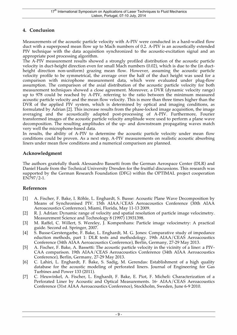
4. Conclusion Measurements of the acoustic particle velocity with A-PIV were conducted in a hard-walled flow duct with a superposed mean flow up to Mach numbers of 0.2. A-PIV is an acoustically extended PIV technique with the data acquisition synchronized to the acoustic-excitation signal and an appropriate post processing algorithm. The A-PIV measurement results showed a strongly profiled distribution of the acoustic particle velocity in duct-height direction even for small Mach numbers (0.02), which is due to the (in duct-height direction non-uniform) grazing mean flow. However, assuming the acoustic particle velocity profile to be symmetrical, the average over the half of the duct height was used for a comparison with microphone measurement data, which were evaluated under plug-flow assumption. The comparison of the axial distribution of the acoustic particle velocity for both measurement techniques showed a close agreement. Moreover, a DVR (dynamic velocity range) up to 978 could be reached by A-PIV, referring to the ratio between the minimum measured acoustic particle velocity and the mean flow velocity. This is more than three times higher than the DVR of the applied PIV system, which is determined by optical and imaging conditions, as formulated by Adrian [2]. This increase results from the phase-locked image acquisition, the image averaging and the acoustically adapted post-processing of A-PIV. Furthermore, Fourier transformed images of the acoustic particle velocity amplitude were used to perform a plane wave decomposition. The resulting amplitudes of the up- and downstream propagating waves match very well the microphone-based data. In results, the ability of A-PIV to determine the acoustic particle velocity under mean flow conditions could be proven. As a next step, A-PIV measurements on realistic acoustic absorbing liners under mean flow conditions and a numerical comparison are planned. Acknowledgment The authors gratefully thank Alessandro Bassetti from the German Aerospace Center (DLR) and Daniel Haufe from the Technical University Dresden for the fruitful discussions. This research was supported by the German Research Foundation (DFG) within the OPTIMAL project cooperation EN797/2-1. References [1] A. Fischer, F. Bake, I. Röhle, L. Enghardt, S. Busse: Acoustic Plane Wave Decomposition by

Means of Synchronised PIV. 15th AIAA/CEAS Aeroacoustics Conference (30th AIAA Aeroacoustics Conference), Miami, Florida, May 11-13 2009.

[2] R. J. Adrian: Dynamic range of velocity and spatial resolution of particle image velocimetry. Measurement Science and Technology 8 (1997) 13931398.

[3] M. Raffel, C. Willert, S. Wereley, J. Kompenhans: Particle image velocimetry: A practical guide. Second ed. Springer, 2007.

[4] S. Busse-Gerstengarbe, F. Bake, L. Enghardt, M. G. Jones: Comparative study of impedance eduction methods, part 1: DLR tests and methodology. 19th AIAA/CEAS Aeroacoustics Conference (34th AIAA Aeroacoustics Conference), Berlin, Germany, 27-29 May 2013.

[5] A. Fischer, F. Bake, A. Bassetti: The acoustic particle velocity in the vicinity of a liner: a PIV-CAA comparison. 19th AIAA/CEAS Aeroacoustics Conference (34th AIAA Aeroacoustics Conference), Berlin, Germany, 27-29 May 2013.

[6] C. Lahiri, L. Enghardt, F. Bake, S. Sadig, M. Gerendas: Establishment of a high quality database for the acoustic modeling of perforated liners. Journal of Engineering for Gas Turbines and Power 133 (2011).

[7] C. Heuwinkel, A. Fischer, L. Enghardt, F. Bake, E. Piot, F. Micheli: Characterization of a Perforated Liner by Acoustic and Optical Measurements. 16th AIAA/CEAS Aeroacoustics Conference (31st AIAA Aeroacoustics Conference), Stockholm, Sweden, June 6-9 2010.

Documents

Measurement of the acoustic particle velocity under