Embed Size (px)
Citation preview

Measurement of Spin-OrbitAlignment in an Extrasolar
Planetary System
Mark Richardson
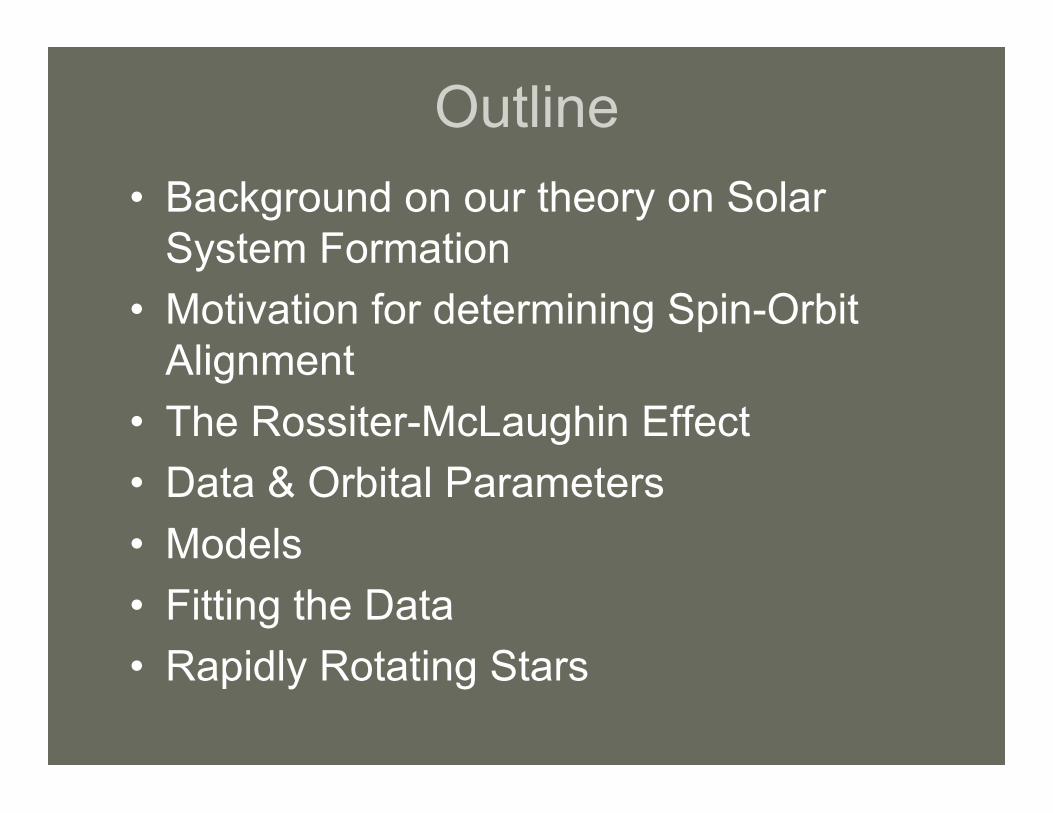
Outline• Background on our theory on Solar
System Formation• Motivation for determining Spin-Orbit
Alignment• The Rossiter-McLaughin Effect• Data & Orbital Parameters• Models• Fitting the Data• Rapidly Rotating Stars

Solar SystemFormation*
*See “Solar System Formation” by Mark Richardson
• Initial rotation(angularmomentum) requiresinitial cloud tocollapse to disk

Motivation• The leading theory on solar system formation
predicts a common angular momentum vector forthe initial and final constituents of the cloud.
• A significant example of this is that the net orbitalangular momenta is expected to point in the samedirection as the solar rotation angular momentum

Motivation Continued
• To find support for this theory, we candetermine the angular difference (ψ)between the orbital angular momentumvector (Ω) and the star’s rotation vector(Ω*).
• Question: Is ψ roughly zero? Comparewith the sun: ~6o (Winn et. al. 2005)

Further Motivation
• Finding ψ ≈ 0 would support the leadingtheory.
• Also it would suggest a way todetermine Ω provided Ω* can be found(consider line broadening, rotationperiod, and stellar radius).
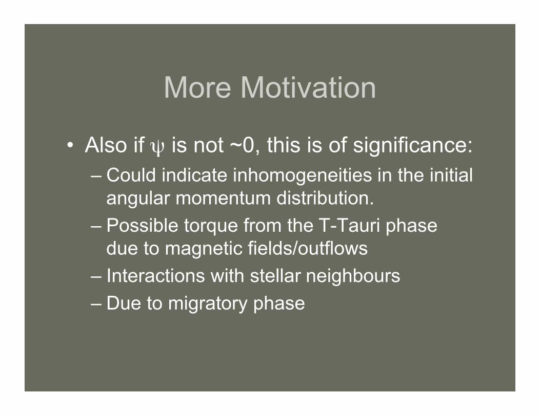
More Motivation
• Also if ψ is not ~0, this is of significance:– Could indicate inhomogeneities in the initial
angular momentum distribution.– Possible torque from the T-Tauri phase
due to magnetic fields/outflows– Interactions with stellar neighbours– Due to migratory phase

Methods
• There are two methods to determine ψthat will be discussed here:– For slowly rotating stars, we can take
advantage of The Rossiter-McLaughlinEffect*.
– For rapidly rotating stars,we can considerthe von Zeipel Theorem*
*Description to come
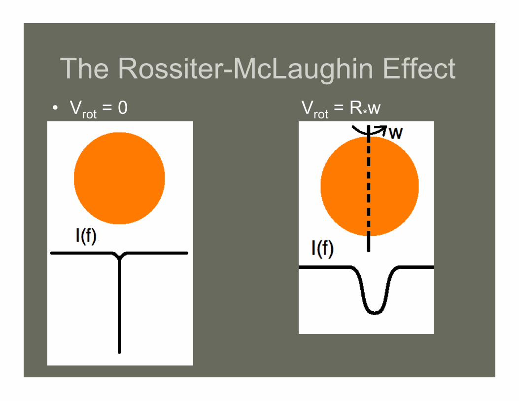
The Rossiter-McLaughin Effect• Vrot = 0 Vrot = R*w

RM Effect
• The obstruction of theblue shiftedfrequencies result inan apparent skewingof the wave towardsthe red.
• This results in anapparent velocity(velocity anomaly) Δv

Finding ψ
• So what does this have to do with ψ … thisis not an easy answer although it issomewhat intuitive … due to technologicaldifficulty I must turn to the whiteboard.

Finding ψ
• So the 3D angle, ψ, is related to the 2Dprojected angle, λ, by:cosψ = cosI*cosI+sinI*sinIcosλ
• I = inclination between orbital plane andsky plane
• I* = inclination between star rotation axisand sky plane
Caveats• Everything is hampered by I and I* (for
example can only find vrotsinI*).• Will only detect a lag-time between t(Δ
v=0) and t(dI/dt=0) provided I≠90o andI*≠0.
• The velocity anomaly is small relativeto the radial velocity observed for theorbital motion, thus a bright host star isrequired to allow for high precision data.

HD 209458
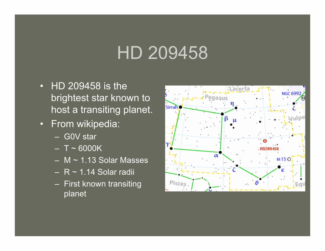
• HD 209458 is thebrightest star known tohost a transiting planet.
• From wikipedia:– G0V star– T ~ 6000K– M ~ 1.13 Solar Masses– R ~ 1.14 Solar radii– First known transiting
planet

Data• 1) 85 sets of spectra data from Laughlin
et al. (2005) between Nov 1999 andDec 2004. Used technique from Butleret. al. (1996) to determine radialvelocities with ~3 to 4m/s accuracy
• 2) 417 photometry datasets from Brownet. al. (2001) with 10-4 relative fluxprecision, including transit data.
Data continued
• 3) IR observations of the secondaryeclipse with signal to noise ratio of ~5 to6.
Parameters
• The article discusses severalparameters. Quickly listed:– Orbital: Mp, P, e, ω,I,λ, ΔtI, X, Y, Z– Flux: RP, R*, u1, u2
– Star: M*, vrotsinI*

Courtesy Wikipedia

The Models• Orbit: Two-Body Keplerian Orbit (see your
favourite textbook!)• Flux of star: Limb darkening using:
I(µ) = 1 - u1(1- µ)-u2(1- µ)2 (6)– µ is the cosine of the angle between the sight line
and the surface normal– From this can calculate the flux from a region of
the star (when/where planet is transiting)– I = 1 when the planet is not transiting

The RM Effect• Winn et. al. have made a new way to simulate
the RM effect depending on the planet’sposition in front of the star.
• Their algorithm is as follows:– A: Take solar spectra and modify it to fit HD
209458 properties– B: Repeat A, only Dopler Shift by vp and stretch
according to fp.– Take A - B, multiply by solar iodine absorption– Convolve with ‘point-spread’ function and put in to
method used to get radial velocities Butler et. al.(1996)
RM Effect
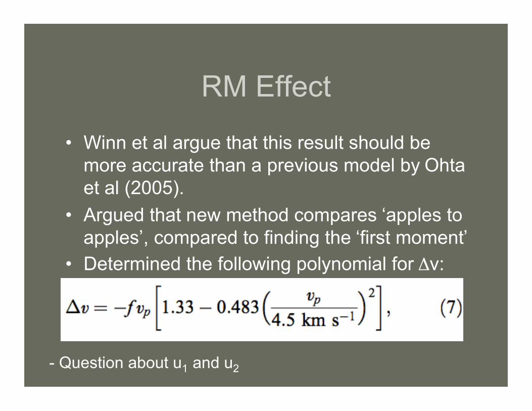
• Winn et al argue that this result should bemore accurate than a previous model by Ohtaet al (2005).
• Argued that new method compares ‘apples toapples’, compared to finding the ‘first moment’
• Determined the following polynomial for Δv:
- Question about u1 and u2


Fitting the Data
• Winn et al are now set to produce simulateddata once they set the parameters describedbefore.
• Method:– Set M*– perform simulations for some set of parameters
(12 of them!)– Determine simulated observations at the same
time as the data– Determine χ2 (to be defined), keep if min. Repeat

Fitting the Data
• The set of parameters that minimize χ2
are taken as the best fit.• Confidence levels are determined by
‘bootstrap Monte Carlo analysis’– Mark: This one’s on you …
• Did this for 100 000 synthetic datasets
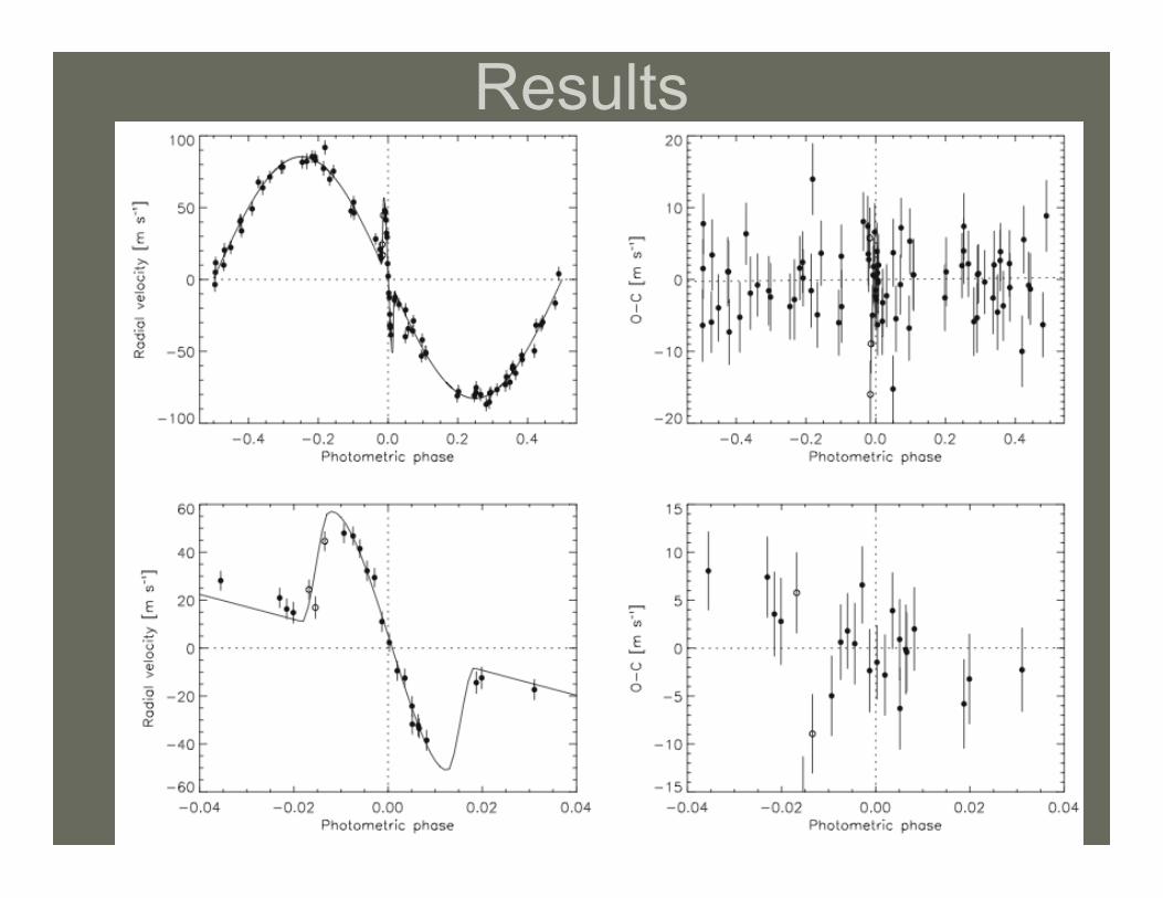
Results

Results


Results
Further Results andDiscussion
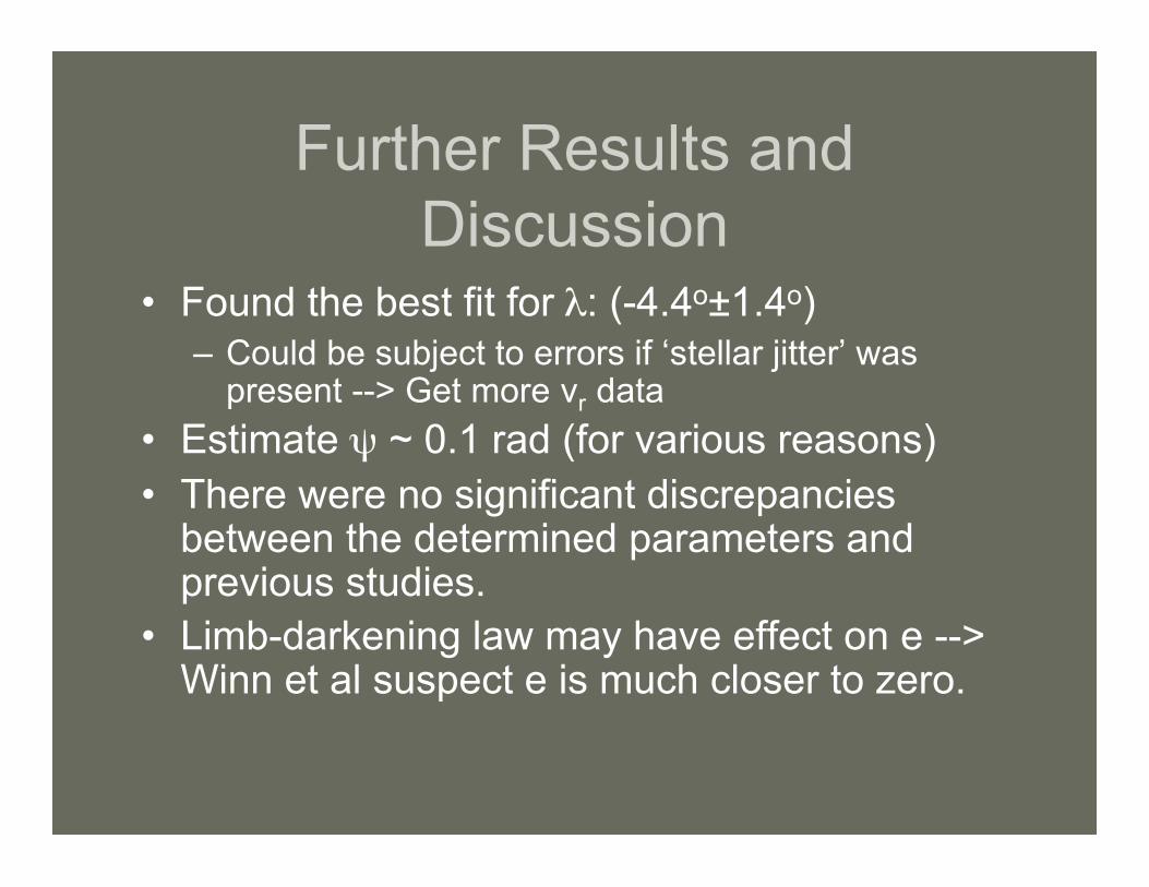
• Found the best fit for λ: (-4.4o±1.4o)– Could be subject to errors if ‘stellar jitter’ was
present --> Get more vr data• Estimate ψ ~ 0.1 rad (for various reasons)• There were no significant discrepancies
between the determined parameters andprevious studies.
• Limb-darkening law may have effect on e -->Winn et al suspect e is much closer to zero.
Further results
• The ψ result gives support for there tobe agreement between Ω and Ω* evenfor smaller orbits (the planet in questionhas a semi-major axis ~ 1/9 Mercury’s)

Cause of ψ
• Winn et al discuss several causes ofdeveloping the angle ψ in a planetarysystem - determine most areimprobable due to very long timescales.
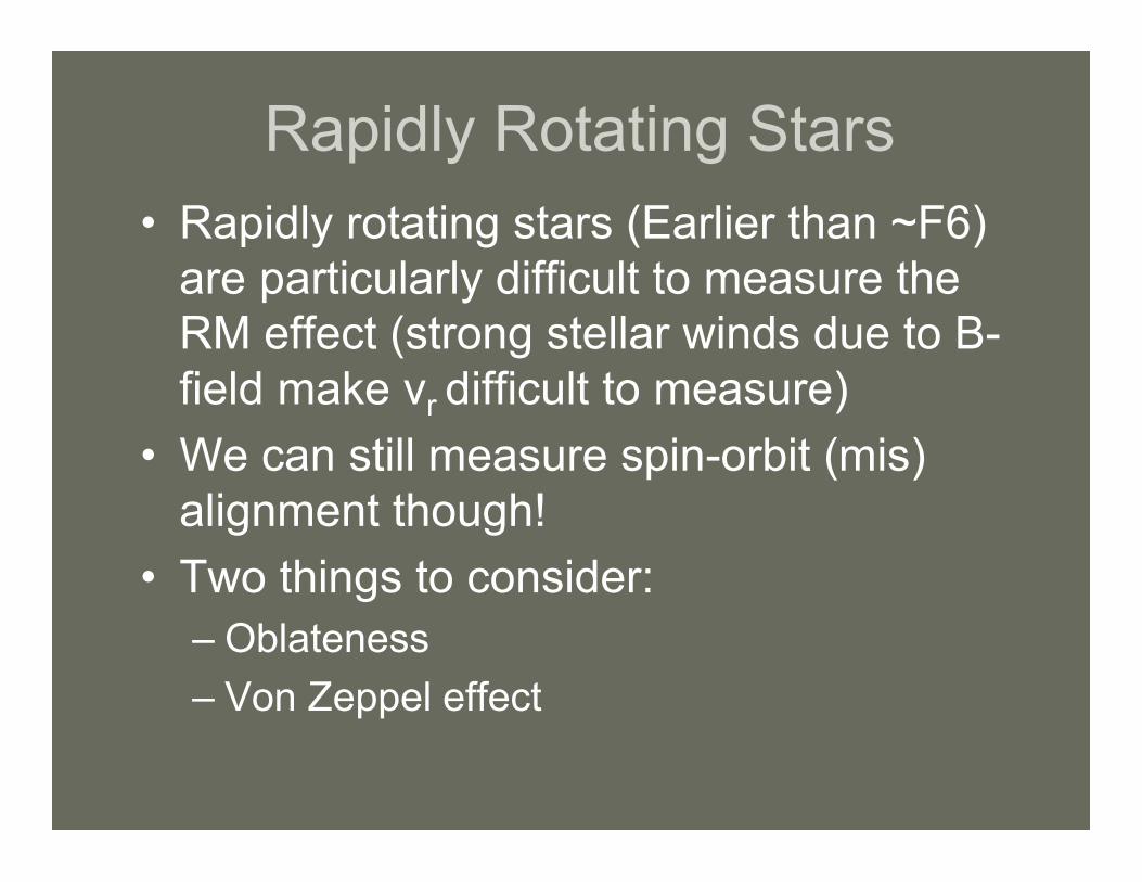
Rapidly Rotating Stars• Rapidly rotating stars (Earlier than ~F6)
are particularly difficult to measure theRM effect (strong stellar winds due to B-field make vr difficult to measure)
• We can still measure spin-orbit (mis)alignment though!
• Two things to consider:– Oblateness– Von Zeppel effect
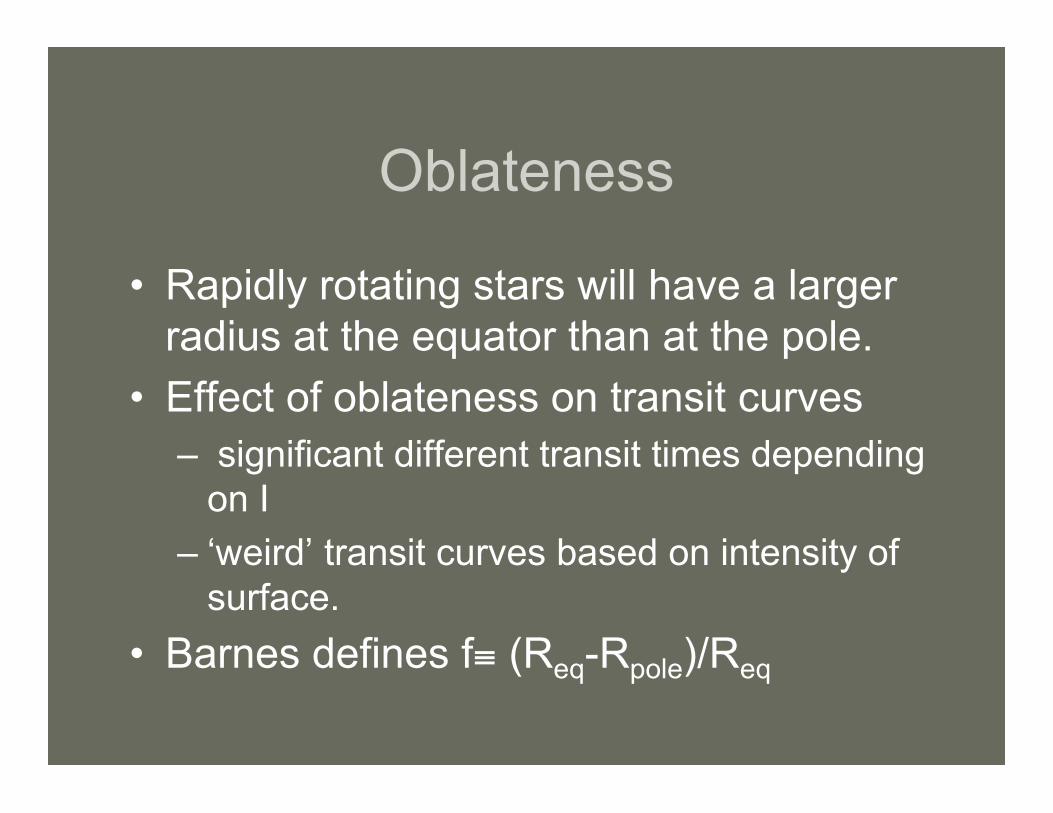
Oblateness
• Rapidly rotating stars will have a largerradius at the equator than at the pole.
• Effect of oblateness on transit curves– significant different transit times depending
on I– ‘weird’ transit curves based on intensity of
surface.• Barnes defines f≡ (Req-Rpole)/Req

Intensity
• Barnes determines surface flux byintegrating over the oblate star (notassuming spherical symmetry)
• Attains this by ‘popping’ the coordinatesinto coordinate space. Only real effecton relative transit fluxes is lumped intothe Intensity in the new coordinates.

Von Zeppel Effect
• Where g is the surface gravity, and β is0.25 for a pure radiative star.
• g is dependant on both gravity and thecentrifugal term.
• From here just use Steffan-Boltzmann’slaw
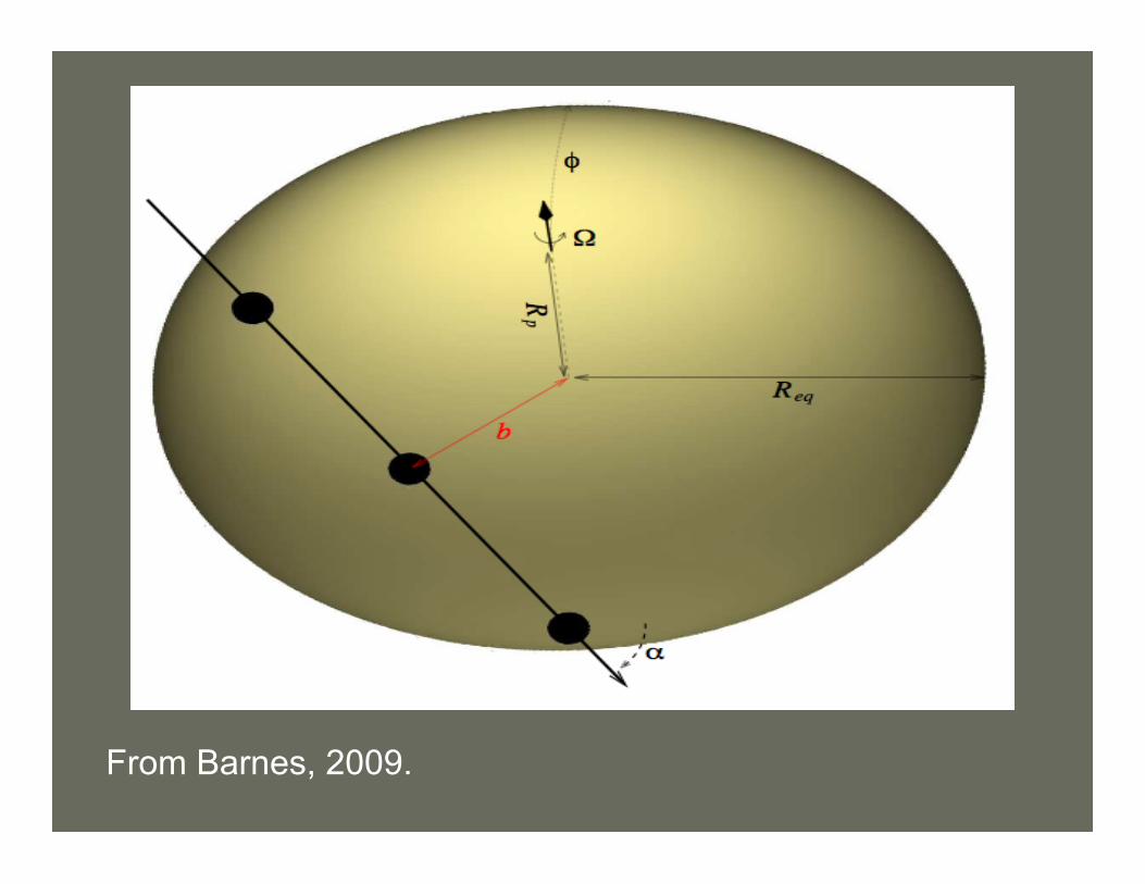
From Barnes, 2009.

α = 0, φ=0

α = 60, φ=30o

α = 60, φ=30o
Conclusion• Barnes has produced intensity plots at
various wavelengths for an assortmentof orbital parameters. It is his hope thatthese will allow for quick comparisonwith results from the Kepler mission.
• I’m curious why he went for suchsignificant variation in α. I see it asmore beneficial to do this detailed workfor α ~ 0 as is expected from our theory.

Conclusions
• We now have seen simulatedobservations for spin-orbit(mis)alignments for both slowly andrapidly rotating stars.
• The RM effect is an efficient tool toanalyze the spin-orbit alignment andhas been used for subsequent stars(see list in Barnes)

Thanks!
• Discussion???

Ecentricity