Embed Size (px)
Citation preview
PHYSICAL REVIEW A, VOLUME 64, 052312
Measurement of qubits
Daniel F. V. James,1,* Paul G. Kwiat,2,3 William J. Munro,4,5 and Andrew G. White2,4
1Theoretical Division T-4, Los Alamos National Laboratory, Los Alamos, New Mexico 875452Physics Division P-23, Los Alamos National Laboratory, Los Alamos, New Mexico 87545
3Department of Physics, University of Illinois, Urbana-Champaign, Illinois 618014Department of Physics, University of Queensland, Brisbane, Queensland 4072, Australia
5Hewlett-Packard Laboratories, Filton Road, Stoke Gifford, Bristol BS34 8QZ, United Kingdom~Received 20 March 2001; published 16 October 2001!
We describe in detail the theory underpinning the measurement of density matrices of a pair of quantumtwo-level systems~‘‘qubits’’ !. Our particular emphasis is on qubits realized by the two polarization degrees offreedom of a pair of entangled photons generated in a down-conversion experiment; however, the discussionapplies in general, regardless of the actual physical realization. Two techniques are discussed, namely, atomographic reconstruction~in which the density matrix is linearly related to a set of measured quantities! anda maximum likelihood technique which requires numerical optimization~but has the advantage of producingdensity matrices that are always non-negative definite!. In addition, a detailed error analysis is presented,allowing errors in quantities derived from the density matrix, such as the entropy or entanglement of formation,to be estimated. Examples based on down-conversion experiments are used to illustrate our results.
DOI: 10.1103/PhysRevA.64.052312 PACS number~s!: 03.67.2a, 42.50.2p
a
ganartutesy
erowtwth
thatctueso-s
eit
erovsean
tri-enthea-
erical
em-of
ine--ic
gleesachein-
n-
-uesion
eal-of
eri-
orrre-o
I. INTRODUCTION
The ability to create, manipulate, and characterize qutum states is becoming an increasingly important areaphysical research, with implications for areas of technolosuch as quantum computing, quantum cryptography,communications. With a series of measurements on a lenough number of identically prepared copies of a quansystem, one can infer, to a reasonable approximation,quantum state of the system. Arguably, the first such expmental technique for determining the state of a quantumtem was devised by George Stokes in 1852@1#. His famousfour parameters allow an experimenter to determine uniquthe polarization state of a light beam. With the insight pvided by nearly 150 years of progress in optical physics,can consider coherent light beams to be an ensemble oflevel quantum mechanical systems, the two levels beingtwo polarization degrees of freedom of the photons;Stokes parameters allow one to determine the density mdescribing this ensemble. More recently, experimental teniques for the measurement of the more subtle quanproperties of light have been the subject of intensive invtigation ~see Ref.@2# for a comprehensive and erudite expsition of this subject!. In various experimental circumstanceit has been found reasonably straightforward to devissimple linear tomographic technique in which the densmatrix ~or Wigner function! of a quantum state is found froma linear transformation of experimental data. However, this one important drawback to this method, in that the recered state might not correspond to a physical state becauexperimental noise. For example, density matrices forquantum state must be Hermitian, positive semidefinite m
*Corresponding author. Mailing address: Mail stop B-283, LAlamos National Laboratory, Los Alamos NM 87545. FAX:~505!667-1931. Email address: [email protected]
1050-2947/2001/64~5!/052312~15!/$20.00 64 0523
n-ofyd
gemheri-s-
ly-eo-e
erixh-m-
ay
e-of
ya-
trices with unit trace. The tomographically measured maces often fail to be positive semidefinite, especially whmeasuring low-entropy states. To avoid this problem‘‘maximum likelihood’’ tomographic approach to the estimtion of quantum states has been developed@3–7#. In thisapproach the density matrix that is ‘‘mostly likely’’ to havproduced a measured data set is determined by numeoptimization.
In the past decade several groups have successfullyployed tomographic techniques for the measurementquantum mechanical systems. In 1990 Ashburnet al. re-ported the measurement of the density matrix for the nsublevels of then53 level of hydrogen atoms formed following collision between H1 ions and He atoms, in conditions of high symmetry which simplified the tomographproblem@8#. Since then, in 1993 Smitheyet al. made a ho-modyne measurement of the Wigner function of a sinmode of light@9#. Other explorations of the quantum statof single mode light fields have been made by Breitenbet al. @10# and Wuet al. @11#. Other quantum systems whosdensity matrices have been investigated experimentallyclude the vibrations of molecules@12#, the motion of ionsand atoms@13,14#, and the internal angular momentum quatum state of theF54 ground state of a cesium atom@15#.
The quantum states of multiple spin-12 nuclei have been mea
sured in the high-temperature regime using NMR techniq@16#, albeit in systems of such high entropy that the creatof entangled states is necessarily precluded@17#. The mea-surement of the quantum state of entangled qubit pairs, rized using the polarization degrees of freedom of a pairphotons created in a parametric down-conversion expment, was reported by us recently@18#.
In this paper we will examine in detail techniques fquantum state measurement as it applies to multiple colated two-level quantum mechanical systems~or ‘‘qubits’’ inthe terminology of quantum information!. Our particular em-
s
©2001 The American Physical Society12-1
ouesnmde
de
thare
ityuerli-
hesi
tt
woth
i
ndd
-fth:
-rti-ec-
ight
ma-
-
eered
ma-
the
hatthe
rent
on-
g,uchept
this
rix
hat
r
JAMES, KWIAT, MUNRO, AND WHITE PHYSICAL REVIEW A64 052312
phasis is qubits realized via the two polarization degreesfreedom of photons, data from which we use to illustrateresults. However, these techniques are readily applicablother technologies proposed for creating entangled statepairs of two-level systems. Because of the central importaof qubit systems to the emergent discipline of quantum coputation, a thorough explanation of the techniques needecharacterize the qubit states will be of relevance to workin the various diverse experimental fields currently unconsideration for quantum computation technology@19#.This paper is organized as follows. In Sec. II we exploreanalogy with the Stokes parameters, and how they lead nrally to a scheme for measurement of an arbitrary numbetwo-level systems. In Sec. III, we discuss the measuremof a pair of qubits in more detail, presenting the validcondition for an arbitrary measurement scheme and introding the set of 16 measurements employed in our expments. Sec. IV deals with our method for maximum likehood reconstruction and in Sec. V we demonstrate howcalculate the errors in such measurements, and how terrors propagate to quantities calculated from the denmatrix.
II. THE STOKES PARAMETERS AND QUANTUM STATETOMOGRAPHY
As mentioned above, there is a direct analogy betweenmeasurement of the polarization state of a light beam andmeasurement of the density matrix of an ensemble of tlevel quantum mechanical systems. Here we exploreanalogy in more detail.
A. Single qubit tomography
The Stokes parameters are defined from a set of fourtensity measurements@20#: ~i! with a filter that transmits50% of the incident radiation, regardless of its polarizatio~ii ! with a polarizer that transmits only horizontally polarizelight; ~iii ! with a polarizer that transmits only light polarizeat 45° to the horizontal; and~iv! with a polarizer that transmits only right-circularly polarized light. The number ophotons counted by a detector, which is proportional toclassical intensity, in these four experiments is as follows
n05N2
~^HuruH&1^VuruV&!5N2
~^RuruR&1^LuruL&!,
n15N~^HuruH&!
5N2
~^RuruR&1^RuruL&1^LuruR&1^LuruL&!,
n25N~^DuruD&!
5N2
~^RuruR&1^LuruL&2 i ^LuruR&1 i ^RuruL&!,
n35N~^RuruR&!. ~2.1!
05231
ofrtoof
ce-to
rsr
etu-ofnt
c-i-
tosety
hehe-is
n-
;
e
Here uH&, uV&, uD&5(uH&2uV&)/A25exp(ip/4)(uR&1 i uL&)/A2, and uR&5(uH&2 i uV&)/A2 are the kets representing qubits polarized in the linear horizontal, linear vecal, linear diagonal (45°), and right-circular senses resptively, r is the (232) density matrix for the polarizationdegrees of the light~or for a two-level quantum system!, andN is a constant dependent on the detector efficiency and lintensity. TheStokes parameters, which fully characterizethe polarization state of the light, are then defined by
S0[2n05N~^RuruR&1^LuruL&!,
S1[2~n12n0!5N~^RuruL&1^LuruR&!,
S2[2~n22n0!5Ni ~^RuruL&2^LuruR&!,
S3[2~n32n0!5N~^RuruR&2^LuruL&!.~2.2!
We can now relate the Stokes parameters to the densitytrix r by the formula
r51
2 (i 50
3 Si
S0s i , ~2.3!
wheres05uR&^Ru1uL&^Lu is the single qubit identity operator ands15uR&^Lu1uL&^Ru, s25 i uL&^Ru2uR&^Lu, ands35uR&^Ru2uL&^Lu are the Pauli spin operators. Thus thmeasurement of the Stokes parameters can be considequivalent to a tomographic measurement of the densitytrix of an ensemble of single qubits.
B. Multiple beam Stokes parameters: Multiple qubittomography
The generalization of the Stokes scheme to measurestate of multiple photon beams~or multiple qubits! is reason-ably straightforward. One should, however, be aware timportant differences exist between the one-photon andmultiple photon cases. Single photons, at least in the curcontext, can be described in a purelyclassicalmanner, andthe density matrix can be related to the purely classical ccept of the coherency matrix@21#. For multiple photons onehas the possibility of nonclassical correlations occurrinwith quintessentially quantum mechanical phenomena sas entanglement being present. We will return to the concof entanglement and how it may be measured later inpaper.
An n-qubit state is characterized by a density matwhich may be written as follows:
r51
2n (i 1 ,i 2 , . . . ,i n50
3
r i 1 ,i 2 , . . . ,i ns i 1
^ s i 2^ •••^ s i n
,
~2.4!
where the 4n parametersr i 1 ,i 2 , . . . ,i nare real numbers. The
normalization property of the density matrices requires tr 0,0, . . . ,051, and so the density matrix is specified by 4n
21 real parameters. The symbol represents the tenso
2-2
surements
rization
MEASUREMENT OF QUBITS PHYSICAL REVIEW A64 052312
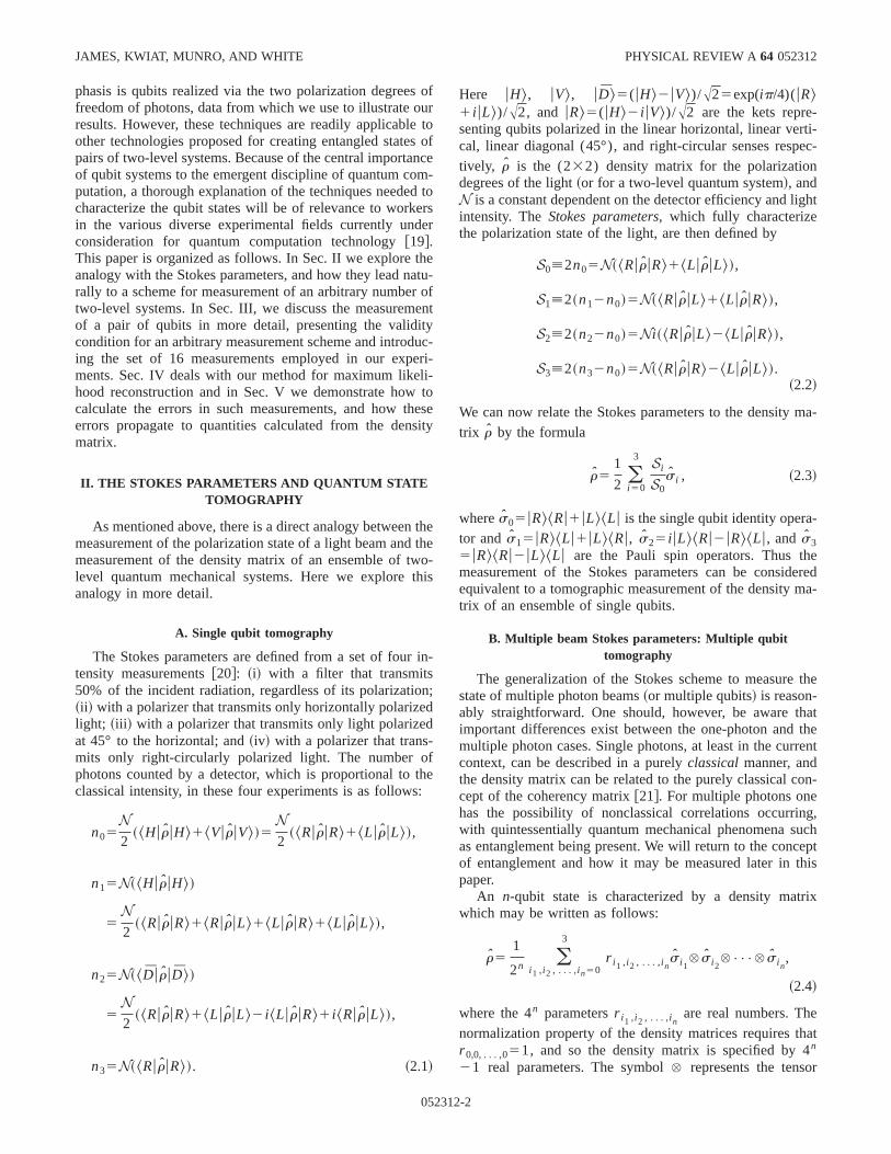
FIG. 1. Tree diagram representing number and type of measurements necessary for tomography. For a single qubit, the mea
$m0 ,m1 ,m2 ,m3% suffice to reconstruct the state, e.g., measurements of the horizontal, vertical, diagonal, and right-circular pola
components, (H,V,D,R). For two qubits, 16 double-coincidence measurements are necessary ($m0m0 ,m0m1 , . . . ,m3m3%), increasing to 64
three-coincidence measurements for three qubits ($m0m0m0 ,m0m0m1 , . . . ,m3m3m3%), and so on, as shown.
s
dn
t
rs
in
rd
-e
o
-
-he
em-
product between operators acting on the Hilbert spaces aciated with the separate qubits.
As Stokes showed, the state of a single qubit can betermined by taking a set of four projection measuremewhich are represented by the four operatorsm05uH&^Hu1uV&^Vu, m15uH&^Hu, m25uD&^Du, m35uR&^Ru. Simi-larly, the state of two qubits can be determined by the se16 measurements represented by the operatorsm i ^ m j ( i , j50,1,2,3). More generally the state of ann-qubit system canbe determined by 4n measurements given by the operatom i 1
^ m i 2^ •••^ m i n
( i k50,1,2,3 andk51,2, . . . ,n). This‘‘tree’’ structure for multiqubit measurement is illustratedFig. 1.
The proof of this conjecture is reasonably straightforwaThe outcome of a measurement is given by the formula
n5N Tr$rm%, ~2.5!
wherer is the density matrix,m is the measurement operator, and N is a constant of proportionality which can bdetermined from the data. Thus in ourn-qubit case the out-comes of the various measurement are
ni 1 ,i 2 , . . . ,i n5N Tr $r~ m i 1
^ m i 2^ •••^ m i n
!%. ~2.6!
Substituting from Eq.~2.4! we obtain
ni 1 ,i 2 , . . . ,i n5
N2n (
j 1 , j 2 , . . . ,j n50
3
Tr$m i 1s j 1
%
3Tr$m i 2s j 2
%•••Tr$m i ns j n
%r i 1 ,i 2 , . . . ,i n.
~2.7!
As can be easily verified, the single qubit measurementeratorsm i are linear combinations of the Pauli operatorss j ,i.e., m i5( j 50
3 Y i j s j , whereY i j are the elements of the matrix
05231
so-
e-ts
of
.
p-
Y5S 1 0 0 0
1/2 1/2 0 0
1/2 0 1/2 0
1/2 0 0 1/2
D . ~2.8!
Further, we have the relation Tr$s i s j%52d i j ~whered i j isthe Kronecker delta!. Hence Eq.~2.7! becomes
ni 1 ,i 2 , . . . ,i n5N (
j 1 , j 2 , . . . ,j n50
3
Y i 1 j 1Y i 2 j 2
•••Y i nj nr i 1 ,i 2 , . . . ,i n
.
~2.9!
Introducing the left inverse of the matrixY, defined so that(k50
3 (Y21) ikYk j5d i j and whose elements are
Y215S 1 0 0 0
21 2 0 0
21 0 2 0
21 0 0 2
D , ~2.10!
we can find a formula for the parametersr i 1 ,i 2 , . . . ,i nin terms
of the measured quantitiesni 1 ,i 2 , . . . ,i n, viz.,
Nr i 1 ,i 2 , . . . ,i n
5 (j 1 , j 2 , . . . ,j n50
3
~Y21! i 1 j 1~Y21! i 2 j 2
•••~Y21! i nj n
3ni 1 ,i 2 , . . . ,i n
[Si 1 ,i 2 , . . . ,i n. ~2.11!
In Eq. ~2.11! we have introduced then-photon Stokes parameter Si 1 ,i 2 , . . . ,i n
, defined in an analogous manner to tsingle photon Stokes parameters give in Eq.~2.2!.
Since, as already noted,r 0,0, . . . ,051, we can make theidentificationS0,0, . . . ,05N, and so the density matrix for thn-qubit system can be written in terms of the Stokes paraeters as follows:
2-3
cethnnesicri
alth
a
tsinrypeaneewe
of
s oftionnts
izer
xesheto
tes
the
one
ror-a
nss:e
n
vithu
ed
JAMES, KWIAT, MUNRO, AND WHITE PHYSICAL REVIEW A64 052312
r51
2n (i 1 ,i 2 , . . . ,i n50
3 Si 1 ,i 2 , . . . ,i n
S0,0, . . . ,0s i 1
^ s i 2^ •••^ s i n
. ~2.12!
This is a recipe for measurement of the density matriwhich, assuming perfect experimental conditions andcomplete absence of noise, will always work. It is importato realize that the set of four Stokes measureme
$m0 ,m1 ,m2 ,m3% is not unique: there may be circumstancin which it is more convenient to use some other set, whis equivalent. A more typical set, at least in optical expements, is m085uH&^Hu, m185uV&^Vu, m285uD&^Du, m385uR&^Ru.
In the following section we will explore more generschemes for the measurement of two qubits, starting widiscussion, in some detail, of how the measurements aretually performed.
III. GENERALIZED TOMOGRAPHIC RECONSTRUCTIONOF THE POLARIZATION STATE OF TWO PHOTONS
A. Experimental setup
The experimental arrangement used in our experimenshown schematically in Fig. 2. An optical system consistof lasers, polarization elements, and nonlinear optical ctals ~collectively characterized for the purposes of this paas a ‘‘black box,’’! is used to generate pairs of qubits inalmost arbitrary quantum state of their polarization degrof freedom. A full description of this optical system and hosuch quantum states can be prepared can be found in R@22–24#.1 The output of the black box consists of a pair
1It is important to realize that the entangled photon pairs are pduced in anondeterministicmanner: one cannot specify with cetainty when a photon pair will be emitted; indeed there is a smprobability of generating four or six or a higher number of photoThus we can onlypostselectivelygenerate entangled photon pairi.e., one only knows that the state was created after if has bmeasured.
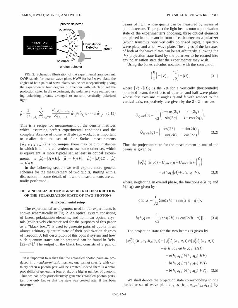
FIG. 2. Schematic illustration of the experimental arrangemeQWP stands for quarter-wave plate,HWP for half-wave plate; theangles of both pairs of wave plates can be set independently githe experimenter four degrees of freedom with which to setprojection state. In the experiment, the polarizers were realizeding polarizing prisms, arranged to transmit vertically polarizlight.
05231
setts
h-
ac-
isgs-r
s
fs.
beams of light, whose quanta can be measured by meanphotodetectors. To project the light beams onto a polarizastate of the experimenter’s choosing, three optical elemeare placed in the beam in front of each detector: a polar~which transmits only vertically polarized light!, a quarter-wave plate, and a half-wave plate. The angles of the fast aof both of the wave plates can be set arbitrarily, allowing tuV& projection state fixed by the polarizer to be rotated inany polarization state that the experimenter may wish.
Using the Jones calculus notation, with the convention
S 0
1D 5uV&, S 1
0D 5uH&, ~3.1!
where uV& (uH&) is the ket for a vertically~horizontally!polarized beam, the effects of quarter- and half-wave plawhose fast axes are at anglesq and h with respect to thevertical axis, respectively, are given by the 232 matrices
UQWP~q!51
A2S i 2cos~2q! sin~2q!
sin~2q! i 1cos~2q!D ,
UHWP~q!5S cos~2h! 2sin~2h!
2sin~2h! 2cos~2h!D . ~3.2!
Thus the projection state for the measurement in one ofbeams is given by
ucpro j(1) ~h,q!&5UQWP~q!•UHWP~h!•S 0
1D5a~h,q!uH&1b~h,q!uV&, ~3.3!
where, neglecting an overall phase, the functionsa(h,q) andb(h,q) are given by
a~h,q!51
A2$sin~2h!2 i sin@2~h2q!#%,
b~h,q!521
A2$cos~2h!1 i cos@2~h2q!#%. ~3.4!
The projection state for the two beams is given by
ucpro j(2) ~h1 ,q1 ,h2 ,q2!&5ucpro j
(1) ~h1 ,q1!& ^ ucpro j(1) ~h2 ,q2!&
5a~h1 ,q1!a~h2 ,q2!uHH&
1a~h1 ,q1!b~h2 ,q2!uHV&
1b~h1 ,q1!a~h2 ,q2!uVH&
1b~h1 ,q1!b~h2 ,q2!uVV&. ~3.5!
We shall denote the projection state corresponding toparticular set of wave plate angles$h1,n ,q1,n ,h2,n ,q2,n% by
-
ll.
en
t.
nges-
2-4

tee
onto
io
inr
thtap
etn
e
le
fece
r,
ci-
for
isonquefor
s ofval-
theeh
ri-tionma-the
inbe
MEASUREMENT OF QUBITS PHYSICAL REVIEW A64 052312
the ketucn&;2 thus the projection measurement is represen
by the operatormn5ucn&^cnu. Consequently, the averagnumber of coincidence counts that will be observed ingiven experimental run is
nn5N^cnurucn& ~3.6!
where r is the density matrix describing the ensemblequbits, andN is a constant dependent on the photon flux adetector efficiencies. In what follows, it will be convenientconsider the quantitiessn defined by
sn5^cnurucn&. ~3.7!
B. Tomographically complete set of measurements
In Sec. II we have given one possible set of projectmeasurements$ucn&^cnu% which uniquely determine thedensity matrixr. However, one can conceive of situationswhich these will not be the most convenient set of measuments to make. Here we address the problem of finding osets of suitable measurements. The smallest number of srequired for such measurements can be found by a simargument: there are 15 real unknown parameters that dmine a 434 density matrix, plus there is the single unknowreal parameterN, making a total of 16.
In order to proceed it is helpful to convert the 434 matrixr into a 16-dimensional column vector. To do this we us
set of 16 linearly independent 434 matrices$Gn% whichhave the following mathematical properties:
Tr$Gn•Gm%5dn,m
A5 (n51
16
GnTr$Gn•A% ;A, ~3.8!
where A is an arbitrary 434 matrix. Finding a set ofGn
matrices is in fact reasonably straightforward: for exampthe set of~appropriately normalized! generators of the Liealgebra SU(2) SU(2) fulfill the required criteria~for refer-ence, we list this set in Appendix A!. These matrices are ocourse simply a relabeling of the two-qubit Pauli matrics i ^ s j ( i , j 50,1,2,3) discussed above. Using these matrithe density matrix can be written as
r5 (n51
16
Gnr n , ~3.9!
wherer n is thenth element of a 16-element column vectogiven by the formula
r n5Tr$Gn• r%. ~3.10!
2Here the first subscript on the wave plate angle refers to onthe two photon beams; the second subscript distinguishes whicthe 16 different experimental states is under consideration.
05231
d
a
fd
n
e-ertesleer-
a
,
ss
Substituting from Eq.~3.9! into Eq. ~3.6!, we obtain thefollowing linear relationship between the measured coindence countsnn and the elements of the vectorr m :
nn5N(m51
16
Bn,mr m ~3.11!
where the 16316 matrixBn,m is given by
Bn,m5^cnuGmucn&. ~3.12!
Immediately we find a necessary and sufficient conditionthe completeness of the set of tomographic states$ucn&%: ifthe matrix Bn,m is nonsingular, then Eq.~3.11! can be in-verted to give
r n5~N !21 (m51
16
~B21!n,mnm . ~3.13!
The set of 16 tomographic states that we employedgiven in Table I. They can be shown to satisfy the conditithatBn,m is nonsingular. By no means are these states uniin this regard: these were the states chosen principallyexperimental convenience.
These states can be realized by setting specific valuethe half- and quarter-wave plate angles. The appropriateues of these angles~measured from the vertical! are given inTable I. Note that overall phase factors do not affectresults of projection measurements.
Substituting Eq.~3.13! into Eq. ~3.9!, we find that
ofof
TABLE I. The tomographic analysis states used in our expements. The number of coincidence counts measured in projecmeasurements provides a set of 16 data that allow the densitytrix of the state of the two modes to be estimated. We have usednotation uD&[(uH&1uV&)/A2, uL&[(uH&1 i uV&)/A2, and uR&[(uH&2 i uV&)/A2. Note that, when the measurements are takenthe order given by the table, only one wave plate angle has tochanged between measurements.
n Mode 1 Mode 2 h1 q1 h2 q2
1 uH& uH& 45° 0 45° 02 uH& uV& 45° 0 0 03 uV& uV& 0 0 0 04 uV& uH& 0 0 45° 05 uR& uH& 22.5° 0 45° 06 uR& uV& 22.5° 0 0 07 uD& uV& 22.5° 45° 0 08 uD& uH& 22.5° 45° 45° 09 uD& uR& 22.5° 45° 22.5° 010 uD& uD& 22.5° 45° 22.5° 45°11 uR& uD& 22.5° 0 22.5° 45°12 uH& uD& 45° 0 22.5° 45°13 uV& uD& 0 0 22.5° 45°14 uV& uL& 0 0 22.5° 90°15 uH& uL& 45° 0 22.5° 90°16 uR& uL& 22.5° 0 22.5° 90°
2-5
dr n-
enityific
JAMES, KWIAT, MUNRO, AND WHITE PHYSICAL REVIEW A64 052312
r5~N !21(n51
16
M nnn5 (n51
16
M nsn , ~3.14!
where the sixteen 434 matricesM n are defined by
M n5 (n51
16
~B21!n,mGm . ~3.15!
The introduction of theM n matrices allows a compact formof linear tomographic reconstruction, Eq.~3.14!, which willbe most useful in the error analysis that follows. TheseM n
matrices, valid for our set of tomographic states, are listeAppendix B, together with some of their important propeties. We can use one of these properties, Eq.~B6!, to obtainthe value of the unknown quantityN. That relationship im-plies
(n
Tr$M n%ucn&^cnur5 r. ~3.16!
Taking the trace of this formula, and multiplying byN weobtain
(n
Tr$M n%nn5N. ~3.17!
For our set of tomographic states, it can be shown that
al
r8
y o
tea
artht
fotb
05231
in-
Tr$M n%5H 1 if n51,2,3,4
0 if n55, . . .,16;~3.18!
hence the value of the unknown parameterN in our experi-ments is given by
N5 (n51
4
nn
5N~^HHuruHH&1^HVuruHV&
1^VHuruVH&1^VVuruVV&!. ~3.19!
Thus we obtain the final formula for the tomographic recostruction of the density matrices of our states:
r5S (n51
16
M nnnD Y S (n51
4
nnD . ~3.20!
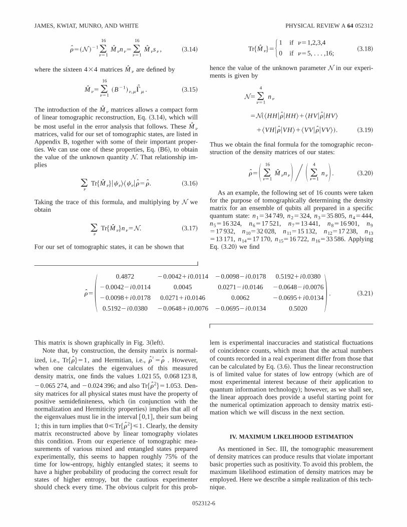
As an example, the following set of 16 counts were takfor the purpose of tomographically determining the densmatrix for an ensemble of qubits all prepared in a specquantum state:n1534 749,n25324, n3535 805,n45444,n5516 324, n6517 521, n7513 441, n8516 901, n9517 932, n10532 028, n11515 132, n12517 238, n13513 171,n14517 170,n15516 722,n16533 586. ApplyingEq. ~3.20! we find
r5S 0.4872 20.00421 i0.0114 20.00982 i0.0178 0.51921 i0.0380
20.00422 i0.0114 0.0045 0.02712 i0.0146 20.06482 i0.0076
20.00981 i0.0178 0.02711 i0.0146 0.0062 20.06951 i0.0134
0.51922 i0.0380 20.06481 i0.0076 20.06952 i0.0134 0.5020
D . ~3.21!
onsers
hatn
to,for
sti-
enttantthebech-
This matrix is shown graphically in Fig. 3~left!.Note that, by construction, the density matrix is norm
ized, i.e., Tr$r%51, and Hermitian, i.e.,r†5 r . However,when one calculates the eigenvalues of this measudensity matrix, one finds the values 1.021 55, 0.068 123
20.065 274, and20.024 396; and also Tr$r2%51.053. Den-sity matrices for all physical states must have the propertpositive semidefiniteness, which~in conjunction with thenormalization and Hermiticity properties! implies that all ofthe eigenvalues must lie in the interval@0,1#, their sum being1; this in turn implies that 0<Tr$r2%<1. Clearly, the densitymatrix reconstructed above by linear tomography violathis condition. From our experience of tomographic mesurements of various mixed and entangled states prepexperimentally, this seems to happen roughly 75% oftime for low-entropy, highly entangled states; it seemshave a higher probability of producing the correct resultstates of higher entropy, but the cautious experimenshould check every time. The obvious culprit for this pro
-
ed,
f
s-edeorer-
lem is experimental inaccuracies and statistical fluctuatiof coincidence counts, which mean that the actual numbof counts recorded in a real experiment differ from those tcan be calculated by Eq.~3.6!. Thus the linear reconstructiois of limited value for states of low entropy~which are ofmost experimental interest because of their applicationquantum information technology!; however, as we shall seethe linear approach does provide a useful starting pointthe numerical optimization approach to density matrix emation which we will discuss in the next section.
IV. MAXIMUM LIKELIHOOD ESTIMATION
As mentioned in Sec. III, the tomographic measuremof density matrices can produce results that violate imporbasic properties such as positivity. To avoid this problem,maximum likelihood estimation of density matrices mayemployed. Here we describe a simple realization of this tenique.
2-6
n-o-
of
MEASUREMENT OF QUBITS PHYSICAL REVIEW A64 052312
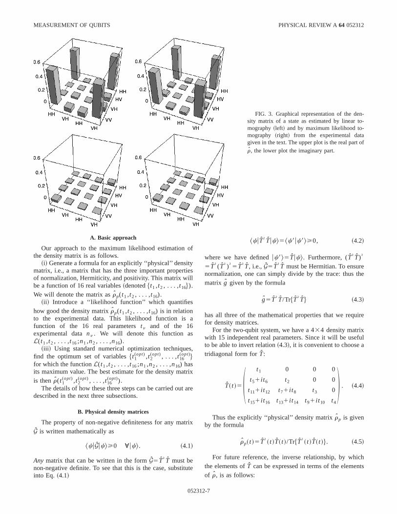
FIG. 3. Graphical representation of the desity matrix of a state as estimated by linear tmography~left! and by maximum likelihood to-mography ~right! from the experimental datagiven in the text. The upper plot is the real part
r, the lower plot the imaginary part.
o
ytiel
a
es
tr
t a
tri
itu
ethe
uire
ful
ichnts
A. Basic approach
Our approach to the maximum likelihood estimationthe density matrix is as follows.
~i! Generate a formula for an explicitly ‘‘physical’’ densitmatrix, i.e., a matrix that has the three important properof normalization, Hermiticity, and positivity. This matrix wilbe a function of 16 real variables~denoted$t1 ,t2 , . . . ,t16%).We will denote the matrix asrp(t1 ,t2 , . . . ,t16).
~ii ! Introduce a ‘‘likelihood function’’ which quantifieshow good the density matrixrp(t1 ,t2 , . . . ,t16) is in relationto the experimental data. This likelihood function isfunction of the 16 real parameterstn and of the 16experimental datann . We will denote this function asL(t1 ,t2 , . . . ,t16;n1 ,n2 , . . . ,n16).
~iii ! Using standard numerical optimization techniqufind the optimum set of variables$t1
(opt) ,t2(opt) , . . . ,t16
(opt)%for which the functionL(t1 ,t2 , . . . ,t16;n1 ,n2 , . . . ,n16) hasits maximum value. The best estimate for the density mais thenr(t1
(opt) ,t2(opt) , . . . ,t16
(opt)).The details of how these three steps can be carried ou
described in the next three subsections.
B. Physical density matrices
The property of non-negative definiteness for any maG is written mathematically as
^cuGuc&>0 ;uc&. ~4.1!
Any matrix that can be written in the formG5T†T must benon-negative definite. To see that this is the case, substinto Eq. ~4.1!
05231
f
s
,
ix
re
x
te
^cuT†Tuc&5^c8uc8&>0, ~4.2!
where we have defineduc8&5Tuc&. Furthermore, (T†T)†
5T†(T†)†5T†T, i.e., G5T†T must be Hermitian. To ensurnormalization, one can simply divide by the trace: thusmatrix g given by the formula
g5T†T/Tr$T†T% ~4.3!
has all three of the mathematical properties that we reqfor density matrices.
For the two-qubit system, we have a 434 density matrixwith 15 independent real parameters. Since it will be useto be able to invert relation~4.3!, it is convenient to choose atridiagonal form forT:
T~ t !5S t1 0 0 0
t51 i t 6 t2 0 0
t111 i t 12 t71 i t 8 t3 0
t151 i t 16 t131 i t 14 t91 i t 10 t4
D . ~4.4!
Thus the explicitly ‘‘physical’’ density matrixrp is givenby the formula
rp~ t !5T†~ t !T~ t !/Tr$T†~ t !T~ t !%. ~4.5!
For future reference, the inverse relationship, by whthe elements ofT can be expressed in terms of the elemeof r, is as follows:
2-7
JAMES, KWIAT, MUNRO, AND WHITE PHYSICAL REVIEW A64 052312
T51A D
M 11(1)
0 0 0
M 12(1)
AM 11(1)M 11,22
(2) AM 11(1)
M 11,22(2)
0 0
M 12,23(2)
Ar44AM 11,22(2)
M 11,23(2)
Ar44AM 11,22(2) AM 11,22
(2)
r44
0
r41
Ar44
r42
Ar44
r43
Ar44
Ar44
2 . ~4.6!
n
inribts
ts
r
al-
theic
n-
wec
d
tion
Here we have used the notationD5Det(r); M i j(1) is the first
minor of r, i.e., the determinant of the 333 matrix formedby deleting thei th row and j th column of r; M i j ,kl
(2) is thesecond minor ofr, i.e., the determinant of the 232 matrixformed by deleting thei th and kth rows and j th and l thcolumns ofr ( iÞk and j Þ l ).
C. The likelihood function
The measurement data consist of a set of 16 coincidecounts nn (n51,2, . . . ,16) whose expected value isnn
5N^cnurucn&. Let us assume that the noise on these cocidence measurements has a Gaussian probability disttion. Thus the probability of obtaining a set of 16 coun$n1 ,n2 , . . .n16% is
P~n1 ,n2 , . . . ,n16!51
Nnorm)n51
16
expF2~nn2nn!2
2sn2 G ,
~4.7!
wheresn is the standard deviation for thenth coincidence
measurement~given approximately byAnn) andNnorm is thenormalization constant. For our physical density matrixrpthe number of counts expected for thenth measurement is
nn~ t1 ,t2 , . . . ,t16!5N^cnurp~ t1 ,t2 , . . . ,t16!ucn&.~4.8!
Thus the likelihood that the matrixrp(t1 ,t2 , . . . ,t16) couldproduce the measured data$n1 ,n2 , . . . ,n16% is
P~n1 ,n2 , . . . ,n16!
51
Nnorm)n51
16
expF2
@N^cnurp~ t1 ,t2 , . . . ,t16!ucn&2nn#2
2N^cnurp~ t1 ,t2 , . . . ,t16!ucn&G , ~4.9!
05231
ce
-u-
whereN5(n514 nn .
Rather than find the maximum value ofP(t1 ,t2 , . . . ,t16)it simplifies things somewhat to find the maximum of ilogarithm ~which is mathematically equivalent!.3 Thus theoptimization problem reduces to finding theminimumof thefollowing function:
L~ t1 ,t2 , . . . ,t16!
5 (n51
16@N^cnurp~ t1 ,t2 , . . . ,t16!ucn&2nn#2
2N^cnurp~ t1 ,t2 , . . . ,t16!ucn&.
~4.10!
This is the ‘‘likelihood’’ function that we employed in ounumerical optimization routine.
D. Numerical optimization
We used theMATHEMATICA 4.0 routine FINDMINIMUM
which executes a multidimensional Powell direction setgorithm~see Ref.@25# for a description of this algorithm!. Toexecute this routine, one requires an initial estimate forvalues oft1 ,t2 , . . . ,t16. For this, we used the tomographestimate of the density matrix in the inverse relation~4.6!,allowing us to determine a set of values fort1 ,t2 , . . . t16.Since the tomographic density matrix may not be nonegative definite, the values of thetn’s deduced in this man-ner are not necessarily real. Thus for our initial guessused the real parts of thetn’s deduced from the tomographidensity matrix.
For the example given in Sec. II, the maximum likelihooestimate is
3Note that here we neglect the dependence of the normalizaconstant ont1 ,t2 , . . . ,t16, which only weakly affects the solutionfor the most likely state.
2-8
MEASUREMENT OF QUBITS PHYSICAL REVIEW A64 052312
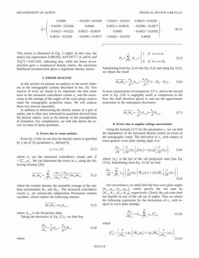
r5S 0.5069 20.02391 i0.0106 20.04122 i0.0221 0.48331 i0.0329
20.02392 i0.0106 0.0048 0.00231 i0.0019 20.02962 i0.0077
20.04121 i0.0221 0.00232 i0.0019 0.0045 20.04251 i0.0192
0.48332 i0.0329 20.02961 i0.0077 20.04252 i0.0192 0.4839
D . ~4.11!
an-um.
ewis
dz
ofoe
er
ed
reom
ate
rs in
les
n
This matrix is illustrated in Fig. 3~right!. In this case, thematrix has eigenvalues 0.986 022, 0.013 977 7, 0, and 0;Tr$r2%50.972 435, indicating that, while the linear recostruction gave a nonphysical density matrix, the maximlikelihood reconstruction gives a legitimate density matrix
V. ERROR ANALYSIS
In this section we present an analysis of the errors inhent in the tomographic scheme described in Sec. III. Tsources of error are found to be important: the shot noerror in the measured coincidence countsnn and the uncer-tainty in the settings of the angles of the wave plates usemake the tomographic projection states. We will analythese two sources separately.
In addition to determining the density matrix of a pairqubits, one is often also interested in quantities derived frthe density matrix, such as the entropy or the entanglemof formation. For completeness, we will also derive therors in some of these quantities.
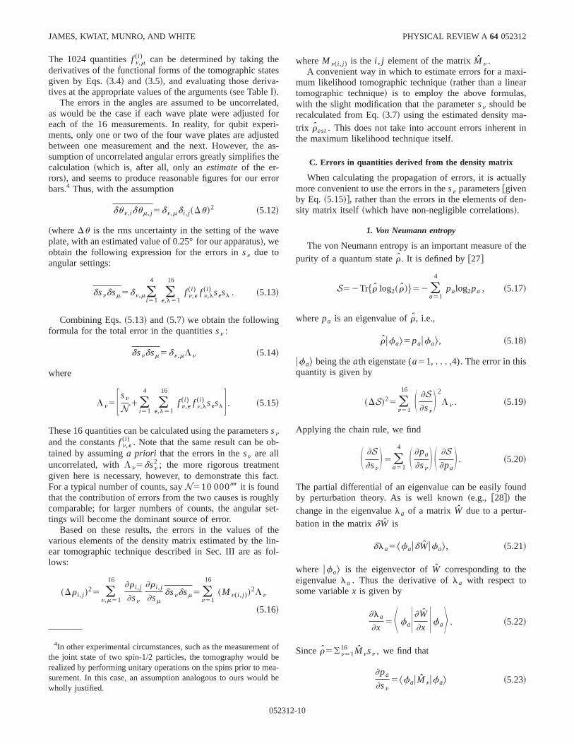
A. Errors due to count statistics
From Eq.~3.20! we see that the density matrix is specifiby a set of 16 parameterssn defined by
sn5nn /N, ~5.1!
where nn are the measured coincidence counts andN5(n51
4 nn . We can determine the errors insn using the fol-lowing formula @26#:
dsndsm5 (l,k51
16 S ]sn
]nlD S ]sm
]nkD dnldnk, ~5.2!
where the overbar denotes the ensemble average of thedom uncertaintiesdsn and dnl . The measured coincidenccounts nl are statistically independent Poissonian randvariables, which implies the following relation:
dnldnk5nldl,k , ~5.3!
wheredl,k is the Kronecker delta.Taking the derivative of Eq.~5.1!, we find that
]sm
]nn5
1
Ndmn2nm
N 2Dn , ~5.4!
where
05231
nd
r-oe
toe
mnt-
an-
Dn5 (l51
4
dl,n5H 1 if 1<n<4
0 if 5<n<16.~5.5!
Substituting from Eq.~5.4! into Eq.~5.2! and using Eq.~5.3!,we obtain the result
dsndsm5nm
N 2dn,m1
nnnm
N 3~12Dm2Dn!. ~5.6!
In most experimental circumstancesN@1, and so the secondterm in Eq. ~5.6! is negligibly small in comparison to thefirst. We shall therefore ignore it, and use the approximexpression in the subsequent discussion:
dsndsm'nm
N 2dn,m[
sm
N dn,m . ~5.7!
B. Errors due to angular settings uncertainties
Using the formula~3.7! for the parameterssn we can findthe dependence of the measured density matrix on errothe tomographic states. The derivative ofsn with respect tosome generic wave plate setting angleu is
]sn
]u5H ]
]u^cnuJ rucn&1^cnurH ]
]uucn&J , ~5.8!
where ucn& is the ket of thenth projection state@see Eq.~3.5!#. Substituting from Eq.~3.14! we find
]sn
]u5 (
m51
16
smF H ]
]u^cnuJ Mmucn&1^cnuMmH ]
]uucn&J G .
~5.9!
For convenience, we shall label the four wave plate ang$h1,n ,q1,n ,h2,n ,q2,n%, which specify the nth state by$un,1 ,un,2 ,un,3 ,un,4%, respectively. Clearly themth state doesnot depend on any of thenth set of angles. Thus we obtaithe following expression for the derivatives ofsn with re-spect to wave plate settings:
]sn
]ul,i5dn,l (
m51
16
sm f n,m( i ) , ~5.10!
where
f n,m( i ) 5H ]
]un,i^cnuJ Mmucn&1^cnuMmH ]
]un,iucn&J .
~5.11!
2-9
ete-
tef
erte
th
rr
ve
rsb
tfa
hlse
thlinfo
xi-
,
-in
lly
n-
the
nd
nbeald
JAMES, KWIAT, MUNRO, AND WHITE PHYSICAL REVIEW A64 052312
The 1024 quantitiesf n,m( i ) can be determined by taking th
derivatives of the functional forms of the tomographic stagiven by Eqs.~3.4! and ~3.5!, and evaluating those derivatives at the appropriate values of the arguments~see Table I!.
The errors in the angles are assumed to be uncorrelaas would be the case if each wave plate were adjustedeach of the 16 measurements. In reality, for qubit expments, only one or two of the four wave plates are adjusbetween one measurement and the next. However, thesumption of uncorrelated angular errors greatly simplifiescalculation~which is, after all, only anestimateof the er-rors!, and seems to produce reasonable figures for our ebars.4 Thus, with the assumption
dun,idum, j5dn,md i , j~Du!2 ~5.12!
~whereDu is the rms uncertainty in the setting of the waplate, with an estimated value of 0.25° for our apparatus!, weobtain the following expression for the errors insn due toangular settings:
dsndsm5dn,m(i 51
4
(e,l51
16
f n,e( i ) f n,l
( i ) sesl . ~5.13!
Combining Eqs.~5.13! and ~5.7! we obtain the followingformula for the total error in the quantitiessn :
dsndsm5dn,mLn ~5.14!
where
Ln5Fsn
N 1(i 51
4
(e,l51
16
f n,e( i ) f n,l
( i ) seslG . ~5.15!
These 16 quantities can be calculated using the parametesn
and the constantsf n,e( i ) . Note that the same result can be o
tained by assuminga priori that the errors in thesn are alluncorrelated, withLn5dsn
2 ; the more rigorous treatmengiven here is necessary, however, to demonstrate thisFor a typical number of counts, sayN510 000-8 it is foundthat the contribution of errors from the two causes is rougcomparable; for larger numbers of counts, the angulartings will become the dominant source of error.
Based on these results, the errors in the values ofvarious elements of the density matrix estimated by theear tomographic technique described in Sec. III are aslows:
~Dr i , j !25 (
n,m51
16]r i , j
]sn
]r i , j
]smdsndsm5 (
n51
16
~M n( i , j )!2Ln
~5.16!
4In other experimental circumstances, such as the measuremethe joint state of two spin-1/2 particles, the tomography wouldrealized by performing unitary operations on the spins prior to msurement. In this case, an assumption analogous to ours wouwholly justified.
05231
s
d,ori-d
as-e
or
-
ct.
yt-
e-l-
whereM n( i , j ) is the i , j element of the matrixM n .A convenient way in which to estimate errors for a ma
mum likelihood tomographic technique~rather than a lineartomographic technique! is to employ the above formulaswith the slight modification that the parametersn should berecalculated from Eq.~3.7! using the estimated density matrix rest. This does not take into account errors inherentthe maximum likelihood technique itself.
C. Errors in quantities derived from the density matrix
When calculating the propagation of errors, it is actuamore convenient to use the errors in thesn parameters@givenby Eq. ~5.15!#, rather than the errors in the elements of desity matrix itself ~which have non-negligible correlations!.
1. Von Neumann entropy
The von Neumann entropy is an important measure ofpurity of a quantum stater. It is defined by@27#
S52Tr$r log2~ r !%52 (a51
4
palog2pa , ~5.17!
wherepa is an eigenvalue ofr, i.e.,
rufa&5paufa&, ~5.18!
ufa& being theath eigenstate (a51, . . . ,4). Theerror in thisquantity is given by
~DS!25 (n51
16 S ]S]sn
D 2
Ln . ~5.19!
Applying the chain rule, we find
S ]S]sn
D5 (a51
4 S ]pa
]snD S ]S
]paD . ~5.20!
The partial differential of an eigenvalue can be easily fouby perturbation theory. As is well known~e.g., @28#! thechange in the eigenvaluela of a matrixW due to a pertur-bation in the matrixdW is
dla5^faudWufa&, ~5.21!
where ufa& is the eigenvector ofW corresponding to theeigenvaluela . Thus the derivative ofla with respect tosome variablex is given by
]la
]x5K faU]W
]xUfaL . ~5.22!
Sincer5(n5116 M nsn , we find that
]pa
]sn5^fauM nufa& ~5.23!
t ofe-be
2-10

ofnnd
ng
gix
spin
eis’’
n the
are
n
tiesment
nc-n-
nly.t
tum
MEASUREMENT OF QUBITS PHYSICAL REVIEW A64 052312
and so, taking the derivative of Eq.~5.17!, Eq. ~5.20! be-comes
S ]S]sn
D52 (a51
4
^fauM nufa&@11 ln pa#
ln 2. ~5.24!
Hence
~DS!25 (n51
16 S (a51
4
^fauM nufa&@11 ln pa#
ln 2 D 2
Ln .
~5.25!
For the experimental example given above,S50.10660.049.
2. Linear entropy
The ‘‘linear entropy’’ is used to quantify the degreemixture of a quantum state in an analytically convenieform, although unlike the von Neumann entropy it hasdirect information theoretic implications. In a normalizeform ~defined so that its value lies between zero and 1!, thelinear entropy for a two-qubit system is defined by
P54
3~12Tr$r2%!5
4
3 S 12 (a51
4
pa2D . ~5.26!
To calculate the error in this quantity, we need the followipartial derivative:
]P]sn
528
3 (a51
4
pa
]pa
]sn
528
3 (a51
4
pa^fauM nufa&
528
3Tr$rM n%
528
3 (m51
16
Tr$MmM n%sm . ~5.27!
Hence the error in the linear entropy is
~DP!25 (n51
16 S ]P]sn
D 2
Ln5(n
16 S 8
3 (m51
16
Tr$MmM n%smD 2
Ln .
~5.28!
For the example given in Secs. III and IV,P50.03760.026.
3. Concurrence, entanglement of Formation, and tangle
The concurrence, entanglement of formation, and tanare measures of the quantum coherence properties of a m
05231
to
leed
quantum state@29#. For two qubits,5 concurrence is defined
as follows: consider the non-Hermitian matrixR5 rSrTSwhere the superscript T denotes the transpose and the ‘‘
flip matrix’’ S is defined by
S5S 0 0 0 21
0 0 1 0
0 1 0 0
21 0 0 0
D . ~5.29!
Note that the definition ofS depends on the basis chosen; whave assumed here the ‘‘computational bas$uHH&,uHV&,uVH&,uVV&%. In what follows, it will be conve-nient to writeR in the following form:
R51
2 (m,n51
16
qm,nsmsn , ~5.30!
where qm,n5MmSM nTS1M nSMm
TS. The left and right
eigenstates and eigenvalues of the matrixR we shall denoteby ^jau, uza&, andr a , respectively, i.e.,
^jauR5r a^jau,
Ruza&5r auza&. ~5.31!
We shall assume that these eigenstates are normalized iusual manner for biorthogonal expansions, i.e.,^jauzb&5da,b . Further we shall assume that the eigenvaluesnumbered in decreasing order, so thatr 1>r 2>r 3>r 4. Theconcurrence is then defined by the formula
C5max$0,Ar 12Ar 22Ar 32Ar 4%
5maxH 0,(a51
4
sgnS 3
22aDAr aJ , ~5.32!
where sgn(x)51 if x.0 and sgn(x)521 if x,0. Thetangle is given byT5C2 and the entanglement of formatioby
E5hS 11A12C2
2 D , ~5.33!
whereh(x)52x log2x2(12x)log2(12x). Becauseh(x) isa monotonically increasing function, these three quantiare to some extent equivalent measures of the entangleof a mixed state.
To calculate the errors in these rather complicated futions, we must employ the perturbation theory for noHermitian matrices~see Appendix C for more details!. Weneed to evaluate the following partial derivative:
5The analysis in this subsection applies to the two-qubit case oMeasures of entanglement for mixedn-qubit systems are a subjecof ongoing research: see, for example,@30# for a recent survey. Itmay be possible to measure entanglement directly, without quanstate tomography; this possibility was investigated in@31#.
2-11
un
is
oulcchlitle
ap
rooue
d.
De-lrch
)q.
JAMES, KWIAT, MUNRO, AND WHITE PHYSICAL REVIEW A64 052312
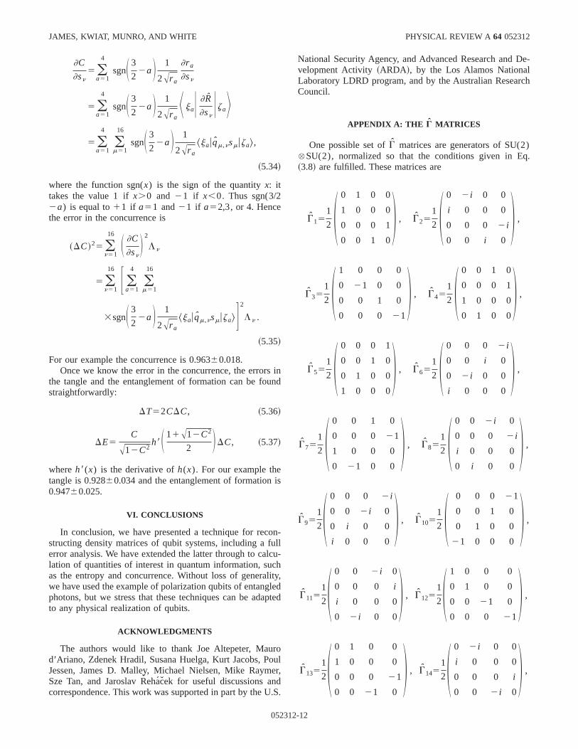
]C
]sn5 (
a51
4
sgnS 3
22aD 1
2Ar a
]r a
]sn
5 (a51
4
sgnS 3
22aD 1
2Ar aK jaU ]R
]snUzaL
5 (a51
4
(m51
16
sgnS 3
22aD 1
2Ar a
^jauqm,nsmuza&,
~5.34!
where the function sgn(x) is the sign of the quantityx: ittakes the value 1 ifx.0 and 21 if x,0. Thus sgn(3/22a) is equal to11 if a51 and21 if a52,3, or 4. Hencethe error in the concurrence is
~DC!25 (n51
16 S ]C
]snD 2
Ln
5 (n51
16 F (a51
4
(m51
16
3sgnS 3
22aD 1
2Ar a
^jauqm,nsmuza&G 2
Ln .
~5.35!
For our example the concurrence is 0.96360.018.Once we know the error in the concurrence, the errors
the tangle and the entanglement of formation can be fostraightforwardly:
DT52CDC, ~5.36!
DE5C
A12C2h8S 11A12C2
2 DDC, ~5.37!
whereh8(x) is the derivative ofh(x). For our example thetangle is 0.92860.034 and the entanglement of formation0.94760.025.
VI. CONCLUSIONS
In conclusion, we have presented a technique for recstructing density matrices of qubit systems, including a ferror analysis. We have extended the latter through to calation of quantities of interest in quantum information, suas the entropy and concurrence. Without loss of generawe have used the example of polarization qubits of entangphotons, but we stress that these techniques can be adto any physical realization of qubits.
ACKNOWLEDGMENTS
The authors would like to thank Joe Altepeter, Maud’Ariano, Zdenek Hradil, Susana Huelga, Kurt Jacobs, PJessen, James D. Malley, Michael Nielsen, Mike RaymSze Tan, and Jaroslav Rˇ ehacek for useful discussions ancorrespondence. This work was supported in part by the U
05231
ind
n-llu-
y,dted
lr,
S.
National Security Agency, and Advanced Research andvelopment Activity ~ARDA!, by the Los Alamos NationaLaboratory LDRD program, and by the Australian ReseaCouncil.
APPENDIX A: THE G MATRICES
One possible set ofG matrices are generators of SU(2^ SU(2), normalized so that the conditions given in E~3.8! are fulfilled. These matrices are
G151
2 S 0 1 0 0
1 0 0 0
0 0 0 1
0 0 1 0
D , G251
2 S 0 2 i 0 0
i 0 0 0
0 0 0 2 i
0 0 i 0
D ,
G351
2 S 1 0 0 0
0 21 0 0
0 0 1 0
0 0 0 21
D , G451
2 S 0 0 1 0
0 0 0 1
1 0 0 0
0 1 0 0
D ,
G551
2 S 0 0 0 1
0 0 1 0
0 1 0 0
1 0 0 0
D , G651
2 S 0 0 0 2 i
0 0 i 0
0 2 i 0 0
i 0 0 0
D ,
G751
2 S 0 0 1 0
0 0 0 21
1 0 0 0
0 21 0 0
D , G851
2 S 0 0 2 i 0
0 0 0 2 i
i 0 0 0
0 i 0 0
D ,
G951
2S 0 0 0 2 i
0 0 2 i 0
0 i 0 0
i 0 0 0
D , G1051
2 S 0 0 0 21
0 0 1 0
0 1 0 0
21 0 0 0
D ,
G1151
2S 0 0 2 i 0
0 0 0 i
i 0 0 0
0 2 i 0 0
D , G1251
2S 1 0 0 0
0 1 0 0
0 0 21 0
0 0 0 21
D ,
G1351
2S 0 1 0 0
1 0 0 0
0 0 0 21
0 0 21 0
D , G1451
2S 0 2 i 0 0
i 0 0 0
0 0 0 i
0 0 2 i 0
D ,
2-12
esic
sen
a
hich
MEASUREMENT OF QUBITS PHYSICAL REVIEW A64 052312
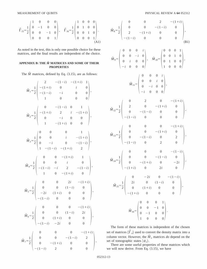
G1551
2 S 1 0 0 0
0 21 0 0
0 0 21 0
0 0 0 1
D , G1651
2 S 1 0 0 0
0 1 0 0
0 0 1 0
0 0 0 1
D .
~A1!
As noted in the text, this is only one possible choice for thmatrices, and the final results are independent of the cho
APPENDIX B: THE M MATRICES AND SOME OF THEIRPROPERTIES
The M matrices, defined by Eq.~3.15!, are as follows:
M151
2 S 2 2~12 i ! 2~11 i ! 1
2~11 i ! 0 i 0
2~12 i ! 2 i 0 0
1 0 0 0
D ,
M251
2 S 0 2~12 i ! 0 1
2~11 i ! 2 i 2~11 i !
0 2 i 0 0
1 2~11 i ! 0 0
D ,
M351
2 S 0 0 0 1
0 0 i 2~11 i !
0 2 i 0 2~12 i !
1 2~12 i ! 2~11 i ! 2
D ,
M451
2 S 0 0 2~11 i ! 1
0 0 i 0
2~12 i ! 2 i 2 2~12 i !
1 0 2~11 i ! 0
D ,
M551
2 S 0 0 2i 2~11 i !
0 0 ~12 i ! 0
22i ~11 i ! 0 0
2~12 i ! 0 0 0
D ,
M651
2 S 0 0 0 2~11 i !
0 0 ~12 i ! 2i
0 ~11 i ! 0 0
2~12 i ! 22i 0 0
D ,
M751
2 S 0 0 0 2~11 i !
0 0 2~12 i ! 2
0 2~11 i ! 0 0
2~12 i ! 2 0 0
D ,
05231
ee.
M851
2 S 0 0 2 2~11 i !
0 0 2~12 i ! 0
2 2~11 i ! 0 0
2~12 i ! 0 0 0
D ,
~B1!
M95S 0 0 0 i
0 0 2 i 0
0 i 0 0
2 i 0 0 0
D , M105S 0 0 0 1
0 0 1 0
0 1 0 0
1 0 0 0
D ,
M115S 0 0 0 i
0 0 i 0
0 2 i 0 0
2 i 0 0 0
D ,
M1251
2 S 0 2 0 2~11 i !
2 0 2~11 i ! 0
0 2~12 i ! 0 0
2~12 i ! 0 0 0
D ,
M1351
2 S 0 0 0 2~11 i !
0 0 2~11 i ! 0
0 2~12 i ! 0 2
2~12 i ! 0 2 0
D ,
M1451
2 S 0 0 0 2~12 i !
0 0 2~12 i ! 0
0 2~11 i ! 0 22i
2~11 i ! 0 2i 0
D ,
M1551
2 S 0 22i 0 2~12 i !
2i 0 ~12 i ! 0
0 ~11 i ! 0 0
2~11 i ! 0 0 0
D ,
M165S 0 0 0 1
0 0 21 0
0 21 0 0
1 0 0 0
D .
The form of these matrices is independent of the cho
set of matrices$Gn% used to convert the density matrix intocolumn vector. However, theM n matricesdo depend on theset of tomographic statesucn&.
There are some useful properties of these matrices wwe will now derive. From Eq.~3.15!, we have
2-13
er
l-
E
ieilhe
io
-ng
tes,
JAMES, KWIAT, MUNRO, AND WHITE PHYSICAL REVIEW A64 052312
^cmuM nucm&5(l
^cmuGlucm&~B21!l,n . ~B2!
From Eq.~3.12! we have^cmuGlucm&5Bm,l ; thus we ob-tain the result
^cmuM nucm&5dm,n . ~B3!
If we denote the basis set for the four-dimensional Hilbspace by$u i & ( i 51,2,3,4)%, then Eq.~3.14! can be written asfollows:
^ i uru j &5(k,l
(n
^ i uM nu j &^cnuk&^ l ucn&^kuru l &. ~B4!
Since Eq.~B4! is valid for arbitrary statesr, we obtain thefollowing relationship:
(n
^ i uM nu j &^cnuk&^ l ucn&5d ikd j l . ~B5!
Contracting Eq.~B5! over the indices (i , j ) we obtain
(n
Tr$M n%ucn&^cnu5 I , ~B6!
whereI is the identity operator for our four-dimensional Hibert space.
A second relationship can be obtained by contracting~B5!, viz.,
(n
^ i uM nu j &5d i j , ~B7!
or, in operator notation,
(n
M n5 I . ~B8!
APPENDIX C: PERTURBATION THEORY FOR NON-HERMITIAN MATRICES
Whereas perturbation theory for Hermitian matricescovered in most quantum mechanics textbooks, the casnon-Hermitian matrices is less familiar, and so we wpresent it here. The problem is as follows. Given teigenspectrum of a matrixR0 @32#, i.e.,
^jauR05r a^jau, ~C1!
R0uza&5r auza&, ~C2!
where
^jauzb&5da,b , ~C3!
we wish to find expressions for the eigenvaluesr a8 and eigen-
states ja8u and uza8& of the perturbed matrixR85R01dR.We start with the standard assumption of perturbat
theory, i.e., that the perturbed quantitiesr a8 , ^ja8u, and uza8&can be expressed as power series of some parameterl:
05231
t
q.
sof
l
n
r a85r a(0)1lr a
(1)1l2r a(2)1•••, ~C4!
uza8&5uza(0)&1luza
(1)&1l2uza(2)&1•••, ~C5!
^ja8u5^ja(0)u1l^ja
(1)u1l2^ja(2)u1•••, ~C6!
Writing R85R01ldR, and comparing terms of equal powers of l in the eigenequations, one obtains the followiformulas:
R0uza(0)&5r a
(0)uza(0)&, ~C7!
^ja(0)uR05r a
(0)^ja(0)u, ~C8!
~R02r a(0)I !uza
(1)&52~dR2r a(1)!uza
(0)&, ~C9!
^ja(1)u~R02r a
(0)I !52^ja(0)u~dR2r a
(1)!. ~C10!
Equations~C7! and ~C8! imply that, as might be expected,
uza(0)&5uza&, ~C11!
^ja(0)u5^jau, ~C12!
r a(0)5r a . ~C13!
Taking the inner product of Eq.~C9! with ^jau, and using thebiorthogonal property Eq.~C3!, we obtain
r a(1)5^jaudRuza&. ~C14!
This implies that
dr a[r a82r a'^jaudRuza&. ~C15!
Thus, dividing both sides by some differential incrementdxand taking the limitdx→0, we obtain
]r a
]x5K jaU ]R
]xUzaL . ~C16!
Using the completeness property of the eigensta(buzb&^jbu5 I , and the identityR05(br buzb&^jbu, we obtainthe following formula
~R02r aI !215 (bÞa
b
1
r b2r auzb&^jbu. ~C17!
Applying this to Eq.~C9! we obtain
udza(1)&[uza8&2uza&'2 (
bÞab
S ^jbudRuza&r b2r a
D uzb&.
~C18!
Similarly, Eqs.~C10! and ~C17! imply
^djau[^dja8u2^djau'2 (bÞa
b
S ^jaudRuzb&r b2r a
D ^jbu.
~C19!
2-14
hi,
y
er
sa-in’98
x-
tt
.
et
sc
at,
ies
,
.
int
00;
n-c
e,
-
on-H.
MEASUREMENT OF QUBITS PHYSICAL REVIEW A64 052312
@1# G.C. Stokes, Trans. Cambridge Philos. Soc.9, 399 ~1852!.@2# U. Leonhardt,Measuring the Quantum State of Light~Cam-
bridge University Press, Cambridge, 1997!.@3# Z. Hradil, Phys. Rev. A55, R1561~1997!.@4# S.M. Tan, J. Mod. Opt.44, 2233~1997!.@5# K. Banaszek, G.M. D’Ariano, M.G.A. Paris, and M.F. Sacc
Phys. Rev. A61, 010304~1999!.@6# Z. Hradil, J. Summhammer, G. Badurek, and H. Rauch, Ph
Rev. A62, 014101~2000!.@7# J. Rehacek, Z. Hradil, and M. Jezˇek, Phys. Rev. A63, 040303
~2001!.@8# J.R. Ashburn, R.A. Cline, P.J.M. Vanderburgt, W.B. West
veld, and J.S. Risley, Phys. Rev. A41, 2407~1990!.@9# D.T. Smithey, M. Beck, M.G. Raymer, and A. Faridani, Phy
Rev. Lett.70, 1244~1993!; see also the discussion of polariztion effects in M.G. Raymer, D.F. McAlister, and A. Funk,Quantum Communication, Computing, and Measurement,edited by P. Kumar~Plenum, New York, 2000!, pp. 147-162.
@10# G. Breitenbach, S. Schiller, and J. Mlynek, Nature~London!387, 471 ~1997!.
@11# J.W. Wu, P.K. Lam, M.B. Gray, and H.-A. Bachor, Opt. Epress3, 154 ~1998!.
@12# T.J. Dunn, I.A. Walmsley, and S. Mukamel, Phys. Rev. Le74, 884 ~1995!.
@13# D. Leibfried, D.M. Meekhof, B.E. King, C. Monroe, W.MItano, and D.J. Wineland, Phys. Rev. Lett.77, 4281~1996!; D.Leibfried, T. Pfau, and C. Monroe, Phys. Today51~4!, 22~1998!.
@14# C. Kurtsiefer T. Pfau, and J. Mlynek, Nature~London! 386,150-153~1997!.
@15# G. Klose, G. Smith, and P.S. Jessen, Phys. Rev. Lett.86, 4721~2001!.
@16# I.L. Chuang, N. Gershenfeld, and M. Kubinec, Phys. Rev. L80, 3408~1998!.
@17# S.L. Braunstein, C.M. Caves, R. Jozsa, N. Linden, S. Popeand R. Schack, Phys. Rev. Lett.83, 1054~1999!.
05231
s.
-
.
.
t.
u,
@18# A.G. White, D.F.V. James, P.H. Eberhard, and P.G. KwiPhys. Rev. Lett.83, 3103~1999!.
@19# A recent overview of many quantum computation technologis given by S. Braunstein and Ho.-K. Lo,Scalable QuantumComputers: Paving the Way to Realization~Wiley, New York,2001!; see also Fortschr. Phys.48, ~9–11! ~2000!.
@20# E. Hecht and A. Zajac,Optics ~Addision-Wesley, ReadingMA, 1974!, Sec. 8.12.
@21# E. Wolf, Nuovo Cimento13, 1165 ~1959!; L. Mandel and E.Wolf, Optical Coherence and Quantum Optics~CambridgeUniversity Press, Cambridge, 1995!, Chap. 6.
@22# P.G. Kwiat, E. Waks, A.G. White, I. Appelbaum, and P.HEberhard, Phys. Rev. A60, R773~1999!.
@23# A.G. White, D.F.V. James, W.J. Munro and P.G. Kwiat, e-prquant-ph/0108088.
@24# A. Berglund, Undergraduate thesis, Dartmouth College, 20A. Berglund, e-print quant-ph/0010001.
@25# W.H. Press, S.A. Teukolsky, W.T. Vetterling, and B.P. Flanery, Numerical Recipes in Fortran 77: The Art of ScientifiComputing, 2nd ed.~Cambridge University Press, Cambridg1992!, Sec. 10.5.
@26# A.C. Melissinos,Experiments in Modern Physics~AcademicPress, New York, 1966!, Sec, 10.4, pp. 467–479.
@27# M.A. Nielsen and I.L. Chuang,Quantum Computation andQuantum Information~Cambridge University Press, Cambridge, 2000!, Chap. 11.
@28# L.I. Schiff, Quantum Mechanics, 3rd ed.~McGraw-Hill, NewYork, 1968!, Eq. ~31.8!, p. 246.
@29# W.K. Wootters, Phys. Rev. Lett.80, 2245~1998!; V. Coffman,J. Kundu, and W.K. Wootters, Phys. Rev. A61, 052306~2000!.
@30# B.M. Terhal, e-print quant-ph/0101032.@31# J.M.G. Sancho and S.F. Huelga, Phys. Rev. A61, 042303
~2000!.@32# The properties of the eigenvectors and eigenvalues of n
Hermitian matrices are discussed by P. M. Morse andFeshbach,Methods of Theoretical Physics~McGraw-Hill, NewYork, 1953!, Vol. I, p. 884et seq.
2-15

![arXiv:1612.02806v2 [quant-ph] 10 Feb 2017takes place by tracing over the qubits representing these nodes (inFigure 1b, this is represented by a measurement on those qubits). Fresh](https://img.dokumen.tips/doc/110x75/5ee3b404ad6a402d666d62d5/arxiv161202806v2-quant-ph-10-feb-2017-takes-place-by-tracing-over-the-qubits.jpg)