arX

iv:q

uant

-ph/

9703

038v

2 2

4 Se

p 19

97

MEASUREMENT IN QUANTUM PHYSICS

Michael Danos ∗

Enrico Fermi Institute,

University of Chicago, Chicago, Illinois 60637, USA

and

Tien D. Kieu †

School of Physics,

University of Melbourne, Parkville, Victoria 3052, Australia

Abstract

The conceptual problems in quantum mechanics – related to the collapse of the wave func-tion, the particle-wave duality, the meaning of measurement – arise from the need to ascribeparticle character to the wave function. As will be shown, all these problems dissolve whenworking instead with quantum fields, which have both wave and particle character. Other-wise the predictions of quantum physics, including Bell’s inequalities, coincide with those ofthe conventional treatments. The transfer of the results of the quantum measurement to theclassical realm is also discussed.

1 Generalities

A vast literature exists on the interpretation of quantum mechanics in general, and on the meaning

of measurement in quantum mechanics in particular. The discussion still takes place today; from

small, semi-popular papers [1] to highly technical large-scale programmatic treatments [2, 3]. To

quote Bell, Ref. [4], who in discussing some of his articles in that book writes in the preface: “these

[articles] show my conviction that, despite numerous solutions of the [measurement] problem ...,

a problem of principle remains.” (See also Feynman, Ref. [5].) The most fundamental of the

problems interfering with the understanding of quantum mechanics is indeed the problem of

measurement, the “genesis of information,” and all the effects surrounding what has been termed

“the Copenhagen collapse of the wave function,” which is not described by the Schrodinger

equation [6]. This process not only lies outside of the framework of quantum mechanics, but,

being instantaneous, also violates relativistic causality. As we will see, all of this is closely related

∗Visiting Scholar.†Present address: CSRIO, Australia.

1

to the so-called “particle-wave duality” and is the source of Bell’s above mentioned “problem of

principle.” Several different proposals to overcome Bell’s above “problem of principle” have been

made. They all in some way break the framework of quantum theory. We shall not discuss these

proposals, but refer the reader to the above mentioned literature citations [1, 2, 3, 4, 6].

Our point is that all problems associated with the subject known as “the problem of mea-

surement in quantum mechanics” can be resolved without abandoning or supplementing quantum

theory. That means that in this context invoking of “new physics” is not needed; even more

strongly, it is counter-indicated.

A separate problem in the measurement process is the need to describe how a result of an

interaction between the measured object and the apparatus on the quantum level is transferred

to the classical level, e.g., to a pointer position. We shall address both these problems in our

paper.

Quite generally, a theory is supposed to be able to make “predictions” in the sense that given

a “state of the system” at some time, say, t0, the theory must be capable of providing information

on the state of the sytem at time t, where t may be later or earlier than t0. The “predictions”

here can apply before the relevant experiment has been performed, or after. Also, the other

terms, e.g., “the state of the system”, are defined within the theory. In quantum physics, which

is our framework, this means (see Sections 7, 8) that given the state of the system as ρ(t0) the

probability of an outcome, Ok(t), is given by TrU(t, t0) ρ(t0) U†(t, t0) Ok(t) where U(t, t0)

is the evolution operator of the system, and where k specifies the outcome. For example, the

outcome could be a particle with spin-up emitted along a particular direction. In general there

are many, usually infinitely many, possible outcomes. However, otherwise quantum physics is

complete in that no hypotheses lying outside of the quantum physics framework are needed, for

any and all circumstances.

Quantum physics does not make predictions on which of the possible outcomes actually will

occur. In particular, it does not predict “when the event (e.g., the decay of the nucleus) actually

will take place.” Such a prediction, being outside of quantum theory, would be in conflict with

the Heisenberg uncertainty relations. One of the attempts to overcome this “limitation of the

theory” is the deBroglie-Bohm pilot wave hypothesis [7]. This attempt supplements the wave

2

function by a “particle function” X(t), called by the authors a “hidden variable.” Even though

outside of quantum mechanics, this work in fact provided the stimulus for Bell to derive the

famous Bell inequalities [8] which allow for the distinction by experiment between at least a large

class of hidden-variable theories and quantum physics. The experiments by now have come out

in favor of the quantum physics predictions [9].

On the other hand, the theory is silent on the choice of the initial conditions. In particular,

one will have to chose t0 sufficiently far back so that the “switching-on” transient is contained

within ones treatment. This is for example the case when investigating the unperturbed [10]

or perturbed [11] non-exponential part of the decay of unstable or metastable states. Another

well-known case is that of the correlations and of the statistics in high-intensity particle beams.

The theory will provide answers for any ρ(t0) and Ok(t) even if the initial conditions actually are

not, and can not be, realized in Nature. The reasons for this impossibility may be obvious, or

may be extremely subtle. A discussion of this is given in Ref. [12]; it lies outside of the scope of

the present paper.

We have used the term “outcome” rather than the usually employed term “measurement”.

The reason for this is that “measurement” seems to imply the participation of an observer. By

using the term “outcome” we want to indicate that one is free to define the system as broad or as

narrow as one likes. Thus one may want to include the observer in the system, which the theory

and the formalism allows; but this choice is irrelevant for our discussion.

In the present essay we want to show that Bell’s conceptual gap [4] disappears when recog-

nizing that the particle-wave duality is only an artifact of quantum mechanics, related to the

absence there of the particle aspects which are amputated when going from quantum field the-

ory to quantum mechanics. The wave function contains only the wave aspects. Quantum fields

(relativistic or non-relativistic) contain simultaneously both the particle and the wave aspects.

The concepts required to construct the needed framework are very few, and very simple. In the

present context the full interacting quantum field theory is not required; one does not have to

go beyond the lowest order, i.e., no Feynman graphs containing loops need be considered. This

limited theory is known to pose no mathematical difficulties [13]. This then is the subject we are

going to address first (in Section 2). Next, in Section 3, we shall show in which way quantum

mechanics (QM) is a sub-field of quantum physics (QP), and then we will be in the position to

3

describe the process of measurement. We do that in the next Sections by analyzing a series of

experiments, and show that both the wave and the particle aspects are needed in the description

of the measurement process. As we will see, no conceptual gaps remain when using both these

aspects. In particular, no split between the quantum system and the conscious experimentalist is

needed; the experimental apparatus, including the experimentalist, can be considered to be part

of the quantum system.

Essentially all of the concepts needed in the description of the measurement in quantum

physics are present already in the case of a two-slit experiment, Section 4, where the measuring

arrangement consists of an array of detectors. The interference pattern which arises in response

to the wave aspect emerges as the result of a large number of experiments, i.e., as a probability

distribution. The particle aspect manifests itself in forbidding coincidences: in a weak beam

situation only one counter at a time can register an event. Here already the “collapse of the

wave function” and “communication at faster than the speed of light” between the counters of

the array has to be operative if one wants to describe the situation in the frame of quantum

mechanics. The last of the concepts, the sensitivity of the interference between different reaction

channels to an intervening measurement, here also can be fully elucidated: a measurement which

determines the slit through which the particle travelled destroys the interference pattern. Such a

measurement changes the two-slit into a single-slit pattern.

The Einstein-Podolski-Rosen (EPR) experiment [14], discussed in Section 5, is the general-

ization of a two-slit experiment to a two-particle system; if one wants to describe it in quantum

mechanics one must replace the 3-dimensional space of the two-slit experiment by a 6-dimensional

configuration space. It requires a somewhat more complex experimental arrangement and also a

more complex theoretical analysis. It is the simplest setup allowing for two-particle coincidences.

When viewed within the frame of quantum mechanics in 3-dimensional position space it has in-

deed the well-known dramatic conceptual problems. Not so in quantum physics: the description

of all these experiments is fully contained within its framework.

In the next two Sections we discuss in detail the completion of the quantum measurement,

i.e., the reaction of a classical system (a pointer, Schrodinger’s cat) to the result in the quantum

system. This involves the description of a classical system in terms of quantum physics; the

mathematics needed for this description is sketched in Appendix A.

4

No split between the “quantum system” and the “classical apparatus” is needed; all has to

be, and can be, considered from the quantum point of view. Another frequently ignored aspect

is that measurement inescapably is an irreversible process, i.e., is associated with dissipation [12]

taking place already on the quantum level. This point is important and must be taken into

account whenever a complete description, including the measuring apparatus, is attempted.

The present paper does not address the question of the logical superstructure, denoted “the

interpretation of quantum mechanics” in Refs. [2, 3]. The arguments and descriptions of these

references in fact involve assumptions concerning the measurement process which are consistent

with, actually follow from, the results of the present paper.

In summary, all aspects required in the description of the evolution of physical systems,

including the act of measurement, are contained within quantum physics. Of course, the 19-th

century dream of a fully deterministic description, which would transcend the frame of quantum

physics, remains unfulfilled.

2 Quantum Physics

In order to make the paper self-contained we now collect the rudimentary aspects of quantum

physics required for the present purpose [13].

In quantum physics the particular state under consideration is described by a state vector,

|S〉. Thus, for example, |S(x1, x2, t)〉 represents a state such that at time t the system had two

particles, one located at x1, the other at x2. The state vector for the system which has no particles

is given the special notation |V 〉, and is denoted as “the vacuum.” The field operator, denoted

by Ψ(x, t), interrogates the state vector for the presence of a particle at the point x, t in the form

Ψ(x, t) |S(y, t)〉 = δ(x − y) |V 〉 (1)

with

Ψ(x, t) | V 〉 = 0 (2)

(in these equations, and throughout in this paper, we shall use units such that h and c = 1).

Hence one calls Ψ a “particle annihilation operator.” Ψ(x, t) and Ψ(x, t) are defined to obey the

5

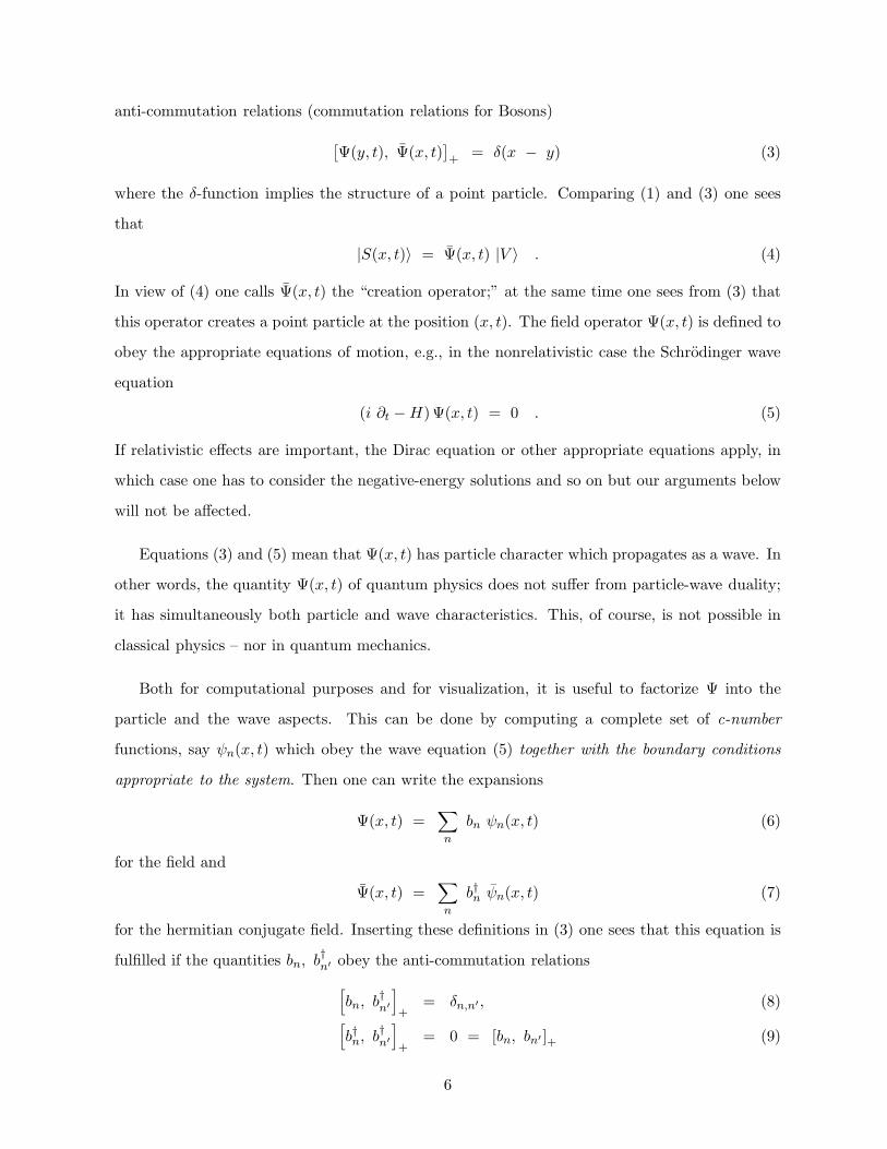
anti-commutation relations (commutation relations for Bosons)

[Ψ(y, t), Ψ(x, t)

]+ = δ(x − y) (3)

where the δ-function implies the structure of a point particle. Comparing (1) and (3) one sees

that

|S(x, t)〉 = Ψ(x, t) |V 〉 . (4)

In view of (4) one calls Ψ(x, t) the “creation operator;” at the same time one sees from (3) that

this operator creates a point particle at the position (x, t). The field operator Ψ(x, t) is defined to

obey the appropriate equations of motion, e.g., in the nonrelativistic case the Schrodinger wave

equation

(i ∂t −H)Ψ(x, t) = 0 . (5)

If relativistic effects are important, the Dirac equation or other appropriate equations apply, in

which case one has to consider the negative-energy solutions and so on but our arguments below

will not be affected.

Equations (3) and (5) mean that Ψ(x, t) has particle character which propagates as a wave. In

other words, the quantity Ψ(x, t) of quantum physics does not suffer from particle-wave duality;

it has simultaneously both particle and wave characteristics. This, of course, is not possible in

classical physics – nor in quantum mechanics.

Both for computational purposes and for visualization, it is useful to factorize Ψ into the

particle and the wave aspects. This can be done by computing a complete set of c-number

functions, say ψn(x, t) which obey the wave equation (5) together with the boundary conditions

appropriate to the system. Then one can write the expansions

Ψ(x, t) =∑

n

bn ψn(x, t) (6)

for the field and

Ψ(x, t) =∑

n

b†n ψn(x, t) (7)

for the hermitian conjugate field. Inserting these definitions in (3) one sees that this equation is

fulfilled if the quantities bn, b†n′ obey the anti-commutation relations

[bn, b

†n′

]

+= δn,n′ , (8)

[b†n, b

†n′

]

+= 0 = [bn, bn′ ]+ (9)

6

which then leads to the completeness relation in the form

∑

n

ψn(x, t) ψn(y, t) = δ(x − y) (10)

for the complete set of the solutions. It is useful to introduce the abbreviation

Ψn(x, t) = bn ψn(x, t) . (11)

Herewith

Ψ(x, t) =∑

n

Ψn(x, t) . (12)

The content of the Eq. (11) can be expressed as: acting on the vacuum the operator Ψn(x, t)

through the operator b†n creates a particle in the state ψn(x, t). Or, said differently, bn is the

particle aspect, and ψn(x, t) is the wave aspect of the quantum physics function Ψn(x, t). For

example, the anticommutation relations (8) ensure that at most one particle can occupy the state

ψn(x, t). In the next Section we will argue that ψn(x, t) is linked to the probability interpretation

of quantum mechanics.

We complete this description by giving the expression for the above-mentioned two-particle

state vector

|S(x1, x2, t)〉 = Ψ(x1, t) Ψ(x2, t) |V 〉 . (13)

On the other hand the state vector of a system having a particle in the state ψn(x, t) is

|Sn〉 = b†n |V 〉 . (14)

Below we will deal mostly with systems of that kind.

3 Quantum Mechanics

The basic concept of quantum mechanics is “the wave function,” also called “the probability

amplitude.” The wave function for the mode n, e.g., the state n of the hydrogen atom, is denoted

as wn(x, t). The meaning of this notation is defined as: given any position x, and any time t,

the value of the wave function is the number wn. The probability of finding the particle there is

then |wn(x, t)|2. To compute the wave function itself one must solve the Schrodinger equation,

or, if relativistic effects are important, the Dirac equation, imposing the appropriate boundary

conditions on the solutions. Both these equations are wave equations.

7

How does this wave function emerge from quantum physics of the last Section? We make the

ansatz

wn(x, t) = 〈V | Ψ(x, t) | Sn〉 , (15)

where

|Sn〉 = b†n |V 〉 (16)

is the state vector for the system in state n. Equations (15) together with (11) yield

wn(x, t) = ψn(x, t) (17)

which turns out to be consistent since both wn(x, t) and ψn(x, t) fulfill the same equation and the

same boundary conditions. This shows that the quantum mechanics wave function is the wave

part of the quantum physics function. The function wn(x, t) describes only “the wave aspects”

of quantum physics; it lacks “the particle aspects” which have been lost in the interrogation

(15). Thus, in contrast to the quantum physics function Ψn(x, t), which describes a particle

propagating, i.e., moving through space and time, the quantum mechanics wave function wn(x, t)

describes a nothing propagating. The latter is a rather abstract entity, having led to many a

fruitless search for the meaning of the deBroglie-Schrodinger wave function, and, with it, the

meaning of quantum mechanics. In order to have a description which contains both the particle

and the wave aspects one needs to work in quantum physics.

4 Preliminary Conclusions and Consolidation

From our discussion above one sees that in quantum physics complementarity, or, as it is also

called, the particle-wave duality, is necessarily absent since the state function (11), Ψn(x, t),

contains simultaneously both aspects. It describes the motion, i.e. the propagation, of a point

particle through space and time. This propagation is that of a wave, which precludes the pos-

sibility of assigning a trajectory to that motion. In contrast, quantum mechanics simply lacks

the particle concept, which is expressed by the interrogation formulae (1), (2), (3). The particle

aspect has been eliminated from quantum mechanics at the point where the wave function was

extracted from the quantum physics function in the interrogation (15). Thus, the quantity which

has been left intact, the wave function wn(x, t), describes the propagation of nothing in particular,

as exemplified by the Cheshire cat, which had left, leaving only the grin behind.

8

In short, only the wave function wn(x, t) exists in quantum mechanics. Of course, the wave

function is an exceedingly rich object, as can be seen from the scope of quantum mechanics.

However, the particle concept is inescapably needed for the understanding, the interpretation, of

the physical content of the results obtained upon computation of the wave function. It therefore

must be re-inserted artificially “by hand.” (In the limited domain “quantum mechanics”, which

does not include, for example, the radiative corrections, in the calculations themselves the particle

aspect is not needed.) This then leads to the particle-wave duality, a logical gap, with the con-

comitant difficulty in reaching full understanding. This gap, which in fact is Bell’s above quoted

“problem of principle”, is one of the factors, most likely the principal factor, which generated the

aura of mystery and fog surrounding the subject “modern physics.”

5 The Two-Slit Experiment

Any measurement requires an interaction between “the system” and the “measuring device”,

and in quantum physics every interaction involves the emission or absorption of a particle (recall

the interaction term ψγµAµψ of quantum electrodynamics: a particle is absorbed in the initial

state and is re-emitted in a different, the final state; a photon is absorbed or emitted). Thus

the measurement process lies outside of the framework of quantum mechanics. Let us discuss

the process of measurement in terms of specific examples. This present discussion will require a

somewhat more technical language than that of the previous Sections.

Consider the determination of a diffraction pattern in a photon two-slit experiment, and

take the low-intensity case to avoid the complication of chance coincidences. The experimental

arrangement thus consists of a photon source, an intervening screen with two (or one) slits, and

an array of detectors behind the slit-screen to register the photons and make the data available

to the experimentalist. The photon field, denoted here by ϕ(x), can be expanded in any set of

solutions of Maxwells equations. Here it will be convenient to employ for the two- and the one-slit

cases two alternative such expansions, namely those which obey the boundary conditions required

to account for the source, screen, two or one slits, etc. In the factorized form of Eqs. (6), (7) the

field then is given by (we change of notation from the previous Sections and suppress the vector

9

character of the photon):

ϕ(x) =∑

n

a(2)n f (2)n (x) ≡∑

n

ϕ(2)n (x) (18)

if both slits are open, and

ϕ(x) =∑

n

a(1)n f (1)n (x) ≡∑

n

ϕ(1)n (x) (19)

if only one slit is open. (Of course, the right-hand sides of Eqs. (18) and (19) can be expanded

in terms of either of f(k)n (x). Expansion in the “wrong” function converges uniformly except in

the vicinity of the slits.) The individual terms of these two sets of solutions, f(2)n (x) , f

(1)n (x) ,

which actually are the wave functions of quantum mechanics, are different since the boundary

conditions for the two cases are different; in particular, the interference patterns described by

these two solutions are different. In these fields, f(k)n (x) concerns the wave aspects, while a

(k)n

concerns the particle aspects: a(k)†n creates, while a

(k)n annihilates, a particle in state f

(k)n (x). The

two parts of the action of the detector, i.e., (i) the interaction with the photons, and (ii) the

registration of a “count” and the transmission of the data to the user, and so on, factorize. The

action (i) of the detector m tests for the presence of a particle by interrogating the state vector at

the space-time point xm (within the resolution of the detector); it is described by the absorption

operator ϕ(xm), both for the single-slit (k = 1) or two-slit (k = 2) case; see. Eqs. (18),(19).

Thus, for instance, the probability amplitude for a particle in state n, being described by the

state vector |S(k)n 〉 = a

(k)†n |V 〉, to be at the point xm, is

〈V |ϕ(k)(xm)|S(k)n 〉 = f (k)n (xm) . (20)

(The also correct form 〈V |ϕ(1)(xm)|S(2)n 〉 is inconvenient in that it results in a linear combination

of the functions f(1)n (xm).) We collect the description of the action (ii) of the detector in an

appropriate operator η, which also includes the detector efficiency. In this way, the action of the

detector at the point xm can be described by the detector function

Dm =∑

n

ηnmϕ(k)n (xm) . (21)

The extent of the sum over n depends on the characteristics of the detector; η also contains the

reaction of the measuring apparatus and hence is an appropriate quantum operator. The actual

construction of the detector is of no importance here; as an example, the absorption of the photon

10

may result in the ionization of an atom, and the emitted electron may initiate a discharge as in

a proportional counter.

For a system having an “incoming” photon in either the two-slit (k = 2) or the one-slit (k = 1)

situation, the probability amplitude for the response of the detector m is

A(k)m = 〈df | ⊗ 〈V |Dm|S(k)

n 〉 ⊗ |di〉 ∼ 〈df |ηnm|di〉 f

(k)n (xm) ; (22)

as to be expected the detector responds to the interference pattern of the photon field, described

by f(k)n (xm). Here 〈df |η|di〉 denotes the expectation value describing the detector response, from

state |di〉 before the interaction to |df 〉 the state after detection. As always, the probability for

counter m to respond is∣∣∣A(k)

m

∣∣∣2.

Both the particle and the wave aspect contributed to the result, Eq. (22). The particle aspect,

the factor ϕ(xm) contained inDm, absorbed/annihilated the photon, and this took place in a local

manner, precisely at the (four-)point xm in the detector m; it also provided the factor f(k)n (x),

i.e., the wave aspect, which is the appropriate solution to Maxwells equations.

Furthermore, once one detector has registered a photon, then no other detector can respond

since the particle already has been absorbed. This follows from the expression for the probability

amplitude, say Ac, of a coincidence in detectors m and m′ (dropping the irrelevant factors),

Ac ∼⟨V |Dm′ Dm| S(k)

n

⟩∼ 〈V |Dm′ | V 〉 = 0 ; (23)

the probability for a coincidence thus vanishes in view of Eq. (2). Expressed in spoken language,

the meaning of Eq. (23) is: “The anwer to the question ‘can two detectors, Dm and Dm′ , absorb

a single particle, S(k)n ?’ is NO.” The absence of a coincidence is enforced by the particle aspect.

The requirement for a “decision” of hitting this one, or that one, but then no other detector,

is the prototype of the need for the “collapse of the wave function” of quantum mechanics, which,

of course, is not described by the equations of motion, e.g., the Schrodinger equation. Namely, in

quantum mechanics the counter m′ must somehow be made to “know” that the counter m has

been hit. The wave function originally in general is non-zero at both places. Thus there is no

reason for counter m′ not to respond at the same time. To avoid such a coincidence one therefore

in quantum mechanics must mimic the uniquely local character of the absorption process. This

is accomplished by “collapsing the wave function”; essentially from f(k)n (xm) to a delta-function

11

at xm – or at xm′ if it was detector m′ which had responded. This “collapse” is even more

spectacular in the case of a more complicated reaction where the wave function extends not only

over a small region of space but over a perhaps large number of reaction channels; to accomplish

this feat “the needed signal: ‘collapse the wave function!’ may have to propagate faster than

light”. (Of course, no such signal is available in quantum theory.) We will return to this point

below in the discussion of the Einstein-Podolski-Rosen experiment.

In case one tries to check “which slit the photon passed through” one has to place a detector

in the slit, say at xs. To know that the photon passed through this slit this detector would have

to record a Compton scattering event. In this detection process the original photon is absorbed

and a new photon is emitted, having a new energy and a new radiation pattern appropriate to

the new geometry (as required by the dependence of the solution on the boundary conditions),

i.e., radiation from within the slit. The Compton detector function then would have the form

Ds ∼ ηs ϕ(−)(s)(xs) ϕ

(k)(xs) (24)

where ϕ(−)(s)(xs) is the emision part of ϕ(xs) for a photon with the new radiation pattern (that

of only one slit open) constructed in analogy to Eqs. (18) or (19). ηs is as previously the operator

describing the reaction of the detector, here the recoiling atom. The new radiation pattern is

different from the old radiation pattern. In particular, it does not exhibit the two-slit interference

pattern.

The two-slit interference pattern will disappear upon the Compton scattering of the photon

even if nobody actually observes the counter, or even if the counter is broken. Such processes,

of course, take place all the time; they are called “collimator scattering” and contribute to the

experimental background. That means that the photon needs not “to know that it has been

observed” to change the interference pattern. This way Nature in quantum physics “has an

objective existence; it exists by itself” independent of observation. Hence the experimental appa-

ratus, and by extension the experimenter, can be considered to be “part of the system”, without

any difficulties, conceptual or otherwise.

Instead of putting a detector in one of the slits to find out which slit the particle passed

through, one may place a screen over one of the slits after the particle has been emitted. This

case requires the description by localized wave-packet states which will be introduced in the next

12

Section. Then, independently of whatever happened before or after, the state of the system is

given by the solution of Maxwells equations appropriate to the boundary conditions valid at the

time when the wave packet arrives at and passes through the slits. The state of the system at

the time when the photon just has been emitted is given as always by

ϕ(x, t) =∑

n

′ C(2)n f (2)n (x)

(a(2)n e−iEt

)+

∑

n

′ C(1)n f (1)n (x)

(a(1)n e−iEt

)(25)

where the coefficients C(2)n and C

(1)n are determined by the emission process. The primes at the

summation signs indicate that the sums are to be taken over the functions appropriate to the

case to avoid double counting. (If the screen with the slits is “very far” from the source, then

C(1)n and C

(2)n may be equal.) The probability for registering a count therefore will contain the

factor∣∣∣C(k)

n

∣∣∣2, multiplying the square of the right-hand side of Eq. (22). Thus, in all of these

experiments, the existence or non-existence of a diffraction pattern or a coincidence is determined

by the particle aspects while the probabilities are given by the wave aspects; and no collapse takes

place or is needed. In other words, the “yes or no” is determined by the particle aspects, the

“how much” by the wave aspects of quantum physics.

6 The E-P-R Experiment

Particularly notorious as a “paradox” is the Einstein-Podolski-Rosen example [8, 14] which in

quantum mechanics for its “explanation” combines the need for wave function collapse and action

at a distance. With respect to the above two-slit example, the EPR setup has two added features

(which lead to complications of detail, but not of principle): (i) the system contains two particles;

and (ii) the time-dependence must be accounted for.

Consider the point (ii) first. An eigenstate of the Hamiltonian by definition has a precise

energy. Hence the wave function of an eigenstate factorizes as

φ(x, t) = e−iEt φ(x) . (26)

The probability to find the particle at the point x, |φ(x, t)|2 = |φ(x)|2, hence is independent of

the time. With this solution thus it is impossible to specify a time as being before, during, or

after the experiment. To achieve this possibility one must chose a suitable superposition of these

13

states. We follow the Weyl prescription. Thus for a free particle we chose the form

w(Ek;x, t) = N∫ Ek+∆

Ek−∆ei[px−E′(t−t0)] dE′ (27)

where N is the normalization constant. This function is localized: it peaks at x = 0 at the time

t = t0; as t increases the peak propagates towards larger x with a velocity the corresponding

classical particle would have. As is well known, one must distinguish between the phase velocity,

a = E/p and the group velocity, b = dE/dp. It is the latter which corresponds to the classical

particle velocity; in view of

p = v√m2 + p2 (28)

and

E =√m2 + p2. (29)

we find b = v. On the other hand a = 1/v. The width ∆ of the superposition determines the

width of the peak in x; also, w(Ek;x, t0) is a minimum-uncertainty wave function.

With functions of this kind one thus can describe, for example, the following: the particle was

emitted from the source at time t0, arrived at the scattering center at time t1, and was absorbed

in the detector at time t2. From now on we will work exclusively with Weyl functions.

We explain the point (i) above directly in terms of the EPR setup. There at time t = t0

two particles of spin s = 1/2, coupled to total spin S = 0, are emitted in opposite directions,

go through a series of polarizers and analyzers to be finally absorbed in two widely separated

detectors. The point of the experiment consists in changing the setup at random after the

particles have been emitted and have become separated by such a distance that “they cannot

communicate” without violating relativistic causality.

We need the following definitions. As the functions w, Eq. (27), form a complete set the field

operator can be expanded as

ϕ(x, t) =∑

an wn(x, t) . (30)

Since we will only deal with the system when the particles are far from the source it is convenient

to split the field into separate field operators for the two directions. Denoting spin “up” and

“down” by the indices + and − respectively, taking the quantization to be along the z-direction,

14

we have for the split field operators (suppressing the time)

ϕw(x) =∑

n

(an+ wn+(x) + an− wn−(x)), x > 0 ; (31)

ϕv(x) =∑

n

(bn+ vn+(x) − bn− vn−(x)), x < 0 . (32)

Thus here w denotes a particle emitted “to the right,” and v “to the left”. Since the particles are

described by Weyl functions they indeed fly apart. The state vector of the system then is

|S2〉 = N (a†n+ b†n− − a†n− b†n+) |V 〉 , (33)

with N the normalization factor; note the absence of the summation over n. In the following we

will suppress the quantum number n for brevity.

The detectors are endowed with polarization analyzers, and are placed at −X and +X re-

spectively with “very large” separation 2|X|. Denoting the polarization of the analyzer by the

subscript p = + or − the detector response is given as

D1 = a+ w+(x) η+ + a− w−(x) η− (34)

and

D2 = b+ v+(x) η′+ + b− v−(x) η

′− (35)

where detector 1 is at x = X and detector 2 at x = −X. The probability for obtaining a

coincidence, i.e., a count in both detectors, irrespective of whether the spin state is “up” or

“down’ then is given by (we suppress the detector states)

A ∼ 〈 V | D1 D2 |S2 〉 . (36)

The quantum probability for detection thus will have an interference term for spins at X opposite

to that at −X, as can be readily deduced from (34).

Now insert a polarization-sensitive filter in arm 1, such that only the “up” state is transmitted.

This filter is represented by the projection operator

F = a†+ a+ (37)

which has the effect given by

F a†+ |V 〉 = a†+ a+ a†+ |V 〉 = a†+ |V 〉 (38)

15

F a†− |V 〉 = a†+ a+ a†− |V 〉 = 0 . (39)

Thus Eq. (36) is replaced by

A ∼ 〈V | D1 D2 F |S2 〉 . (40)

Now only the term with spin “up” at X and “down” at −X survives. That means, that in a

coincidence the detector in arm 1 “determines” the polarization of the particle in arm 2. And

it does not matter at what time the filter was inserted in the beam path, as long as that took

place before the arrival of the Weyl wave packet. All these results emerge directly in terms of the

quantum physics functions; no collapse of a wave function, or transmission of a signal, is required.

To guarantee that, where appropriate, coincidences indeed do occur requires that the detector

efficiencies be 100%.

A similar analysis can be carried out for the case of a spin-flip filter,

T = a†+ a− + a†− a+ , (41)

the action of which is given by

T a†+ |V 〉 = a†− |V 〉 (42)

or

T a†− |V 〉 = a†+ |V 〉 . (43)

Replacing in (40) F by T of (41), one finds that coincidence is achieved when both detected spins

are of the same “orientation”. As above, it does not matter when the filter was inserted. Again,

the counter in one of the arms “determines” the polarization of the particle in the other arm.

The importance of coupling to spin S = 0 is manifested by the minus sign in Eq. (33).

As there is no privileged direction, one can choose the polarization detectors to be sensitive

along the y-direction. Then the detector response function (34) is represented by a′± and b′±, the

annihilation operators quantized along y-orientation. The state vector of the system still can be

represented by (33). However, it now is more convenient to expand the field operator (31) in the

basis of y-oriented wave functions, and the above analysis will go through with “up” and “down”

now referring to the y-axis. Whatever the representation of the field operator, we obtain the same

result.

An interesting case arises when the analyzer of the detector in arm 1 measures the spin along

the z-axis and that of arm 2 along the y-axis, say. The state then would appear to the detector

16

in arm 2 as having terms not only of the form a†+ b′†− but also of the form a†+ b′†+. Therefore no

strict yes-no coincidence rules would exist and only probability predictions would be possible. It

is precisely these probabilities which are different in quantum physics and in classical probability.

The analysis of this situation forms the basis for the Bell inequalities. All of the Bell predictions,

Ref. [8], made in the framework of quantum mechanics are correct, i.e., are in full agreement with

those derivable from the above quantum physics description – except for requiring an acausal

propagation of the hypothetical signal “inducing the collapse of the wave function”.

7 Dissipation and Decoherence in Measurement

Above we demonstrated that the measurement process in quantum physics poses no conceptual

problems when describing it in terms of quantum fields. In that discussion we paid no attention

to the full measurement process, which actually can be split into two interdependent stages: the

interaction with the quantum object, and the chain of amplification to the macroscopic “pointer

position”. The essential point in the second stage is the transfer of the results of the measurement

from the quantum physics (QP) part to the Classical Physics (CP) part of the apparatus.

So far we have concentrated only on the first of these stages, i.e., the very first interaction

between the “system” and the “apparatus”. In the present Section we shall develop a more

complete description, which will allow us to trace the process through to the completion of the

second stage, i.e., from the beginning of the amplification chain to the display of the result of

the measurement by a “pointer position”. Our aim is to derive the expression for the probability,

say Pp, of the pointer position p after the conclusion of the measurement process. In essence this

amounts to the full treatment of the matrix element 〈df |η|di〉 of Eq. (22) postponed in Section 5.

Since the “yes or no” question has been answered in the first of the two stages of the overall

measurement process, the second part which concerns the “how much” aspect could be discussed

simply in the quantum mechanics (QM) framework. For completeness we will, however, also

discuss it in the full QP frame.

The essential new aspects to be treated now will be: (i) the inclusion of dissipation which

is inherent and inevitable in any actual measurement since any elementary quantum act of the

measurement process itself is irreversible, i.e., dissipative [12]; and (ii) the process of decoherence,

17

which, as we will see, is the physical basis for the conversion from a quantum to a classical

process [15, 17]. Superficially, these points seem similar but we will see that actually they differ

in an essential manner. Of these two aspects, in particular (ii) requires that the description be

done in terms of density matrices (see Appendix A), needed when dealing with non-interfering,

“classical” objects. To give a full description we will have to assemble some needed QP quantities,

in particular in the context of decoherence.

Concerning point (i), the very interaction underlying the measurement involves a time-reversal

non-invariant evolution of the system object-plus-device, no matter whether the objects are quan-

tum or classical. The dissipation in the macroscopic, “classical”, down-part of the chain of the

overall process poses no problem. Our subject here thus is the analysis of the dissipation as-

sociated with the elementary, the quantum measurement process at the very beginning of the

chain.

The point (ii) deals with the transition from the quantum to the classical part of the chain.

This involves the description of classical objects in the QP frame. It is essential in resolving the

Schrodinger cat paradox.

Begin with point (i), the initial interaction. For definitiveness we take as the example of the

initial “quantum detector” a Compton proportional counter as used to determine “the slit the

photon went through” in the two-slit experiment of Section 5. Such a counter is filled with a

low-pressure gas and contains the needed electrodes. The photon may suffer Compton scattering

on one of the electrons belonging to one of the gas molecules, the gas being a classical object of

given temperature and pressure. We thus need the quantum description of that classical molecule,

both of its motion and of its internal state, for example its rotation-vibration quantum numbers,

and so on.

Consider the translational motion. Being confined to the counter volume, it can not be

described by a plane wave. Instead, the basis states can be taken as Weyl packets, Eq. (27). Since

it is a classical non-interfering state, it must be described by a density matrix (see Appendix A).

That means, the density matrix must be made up of Weyl basis states, each of which is confined

to the counter volume. Denoting the energy expectation of a Weyl basis state, φi, by Ei, i.e.,

Ei = 〈φi | H | φi〉 , (44)

18

the elements of the density matrix will be

ωij = Z δi,je−Ei/T , (45)

with Z the normalization constant, and T the temperature. In (44) the index i may encompass

the internal quantum numbers of the molecule. (For room temperature and taking the gas of the

counter to be argon we obtain the localization of the atoms, i.e., their position uncertainty, to

be less than atomic dimensions, thus negligibly small.) The form of the density matrix for an

individual molecule thus is of block-diagonal form: each Weyl basis state, being a wave function

as in Eq. (27), is given by a block of fully interfering components, while no interferences exist

between different blocks. The density matrix of the complete system, of the proportional counter,

is given by the direct product of the individual-molecule density matrices.

To continue we need the QP expressions (see Appendix A) corresponding to the QM expres-

sions used above in Eqs. (27), (44), (45). To that end we write the expansion of the Weyl states

in the usual plane wave basis χi:

φi =

∫dpgi(p)χi(p) , (46)

where the functions gi(p) form a suitable complete orthonormal set chosen in particular to ensure

the fulfillment of the boundary conditions, i.e., vanishing outside of the counter. (The form of

Eq. (46) is more general than that of Eq. (27).) Then the QP field operator is written [18]

ψi =∑

i

Biφi , (47)

where Bi is the annihilation operator for the Weyl mode i,

Bi =

∫dpgi(p)bi(p) . (48)

Herewith we can write the (bilinear) state vector for the initial-state density matrix

S (0) =∑

ij

B†i |V 〉 ω

(0)ij 〈V |Bj ≡

∑

ij

S(0)ij . (49)

We shall call these quantities “density state vectors.” Similarly we have mutatis mutandis for the

final state

S (f) =∑

ij

B†i |V 〉 ω

(f)ij 〈V |Bj ≡

∑

ij

S(f)ij , (50)

19

which we will have to compute by considering the evolution of the system.

Denoting the photon Fock-space operators by a(0), a(f) for the initial and final photon state,

respectively, we have for the complete density state vector

S(k) =∑

mn,ij

a(k)†m σ(k)mn S(k)ij a(k)n ≡

∑

mn,ij

S(k)mn,ij (51)

with (k) = (0), (f), and σ(k)mn the photon density matrix.

The interaction with the incoming photon is, as always,

H(x) = ie ψ(x)γµψ(x)Aµ(x) ; (52)

here ψ(x) can be expanded in terms of the functions ψi, Eq. (47). As we are interested in a

Compton process, the full interaction, including the rest of the apparatus, indicated as previously

by η, is

I η = H(y) G(y, x) H(x) η . (53)

Here G is the relevant Green function, describing the propagation of the electron from x to y.

Concerning dissipation in the measurement interaction induced by Eq. (53), every initial state,

i.e., every incoming reaction channel, leads to several, actually to a very large number, of reaction

channels. This is the signature of dissipation, as shown in Ref. [12], and as is immediately visible

from the quantum Boltzmann formula for the entropy E [12]:

E(k) = −∑

j

ω(k)jj log ω

(k)jj (54)

where the superscript (k) indicates the initial or final state. There are very many more states, j,

in the final state than in the initial: the entropy has increased in the measurement interaction. It

does not matter whether the final-state degrees of freedom are observed or not; they participate

in the entropy Eq. (54). (See Ref. [12] concerning irreversibility.)

Now to the point (ii) above, the question of decoherence. That process arises when the full

density matrix is replaced by the “effective” density matrix, i.e., that part of the density matrix

associated with the relevant degrees of freedom, and when in that replacement the density matrix

loses some or all of its off-diagonal elements by tracing over the unobserved degrees of freedom

– which, in fact, is the only possible mechanism for decoherence [15]. (This tracing has the

20

same origin as the integration over the unobserved degrees of freedom when contracting a fully

differential cross section to a partially differential cross section.) This way we expect that for

the final state, being a classical system, the density matrix ω(f)ij also will be diagonal, i.e., fully

decohered. However, since the incoming photon may be in a pure state, that expectation may

not be fulfilled; this has to be investigated.

The complete response of the system, the probability Pp, then is given by the general expres-

sion

Pp = Tr′〈 I†S (0) I R 〉 . (55)

The structure of (55) is: the state after the initial interaction, I†S (0) I, undergoes evolution by

the action of the system evolution operator R, associated with the operator η. We now must

decide how far down the chain of evolution we want to follow. Thus one may include the observer

in the description; this would require knowledge of the QP mechanism of the brain action, which

we do not possess. We shall, however follow the chain in principle – even though not in detail

– down to the “pointer position”. As we will see, it is fully sufficient to break off the QP chain

much earlier, essentially immediately after the elementary act of the quantum measurement, and

continue its description as a CP object.

In Eq. (55) R is written in the density matrix form. Hence, in terms or the Tomonaga –

Schwinger evolution operator, i.e., the U -matrix [13], R is of the form

R = U(t, t0) U†(t, t0) (56)

which is the full QP expression. It gives the state of the system at time t, i.e., the fully differential

transition probability into all channels. To obtain the probability for a particular final state, say,

a given pointer position, one sums over all unobserved degrees of freedom, i.e., one computes the

full trace leaving out the observed variables – hence the prime at the trace symbol. Eq. (55) is a

QP expression.

We recognize that, in the notation of Section 5, the counter m, Eq. (21) will respond for all

(photon) states ϕn(xm) which are non-zero at xm. The different states n are here associated with

different recoils of the atom having undergone the Compton scattering. They provide the initial

states for the evolution operator R, Eq. (56), i.e., the sate of the system at time t0. The operator R

contains the downstream dynamics, in particular the (hypothetical!) recoil detector. Even though

21

in our example of the Compton counter such a detector can not be built, in simpler cases it might

be possible to achieve the appropriate measurement [16]. Then in this step no decoherence would

occur; the interference terms between the reaction channels would be retained. Thus, in contrast

to dissipation, which is inevitable, decoherence is not a basic law of nature.

We now discuss the decoherence in some more detail, considering a system of adequate com-

plexity to qualify as a (potentially) classical apparatus. As the system evolves down the amplifi-

cation chain it not necessarily loses coherence immediately. That can be seen as follows.

Taking the sytem at the beginning of the step c of the chain to be in a pure state, i.e., to be

given by a wave function (for brevity we write here in analogy to Eq. (15) only the wave function

part remaining after the evaluation of the Fock operator matrix elements)

ψ =∑

Ci ϕi (57)

then, at the next step, c′ = c+ 1,

ψ′ =∑

C ′j ϕj (58)

and similarly with c′′ = c+ 2,

ψ′′ =∑

C ′′k ϕk . (59)

The relation between the consecutive density matrices in terms of evolution operator U is

ρ′′kk′ = C ′′k C

′′∗k′

=∑

j,j′

Ukj U∗k′j′ C

′j C

′∗j′ =

∑

j,j′

Ukj U∗k′j′ ρ

′jj′

=∑

j,j′;i,i′

Ukj U∗k′j′ Uji U

∗j′i′ Ci C

∗i′

=∑

j,j′;i,i′

Ukj U∗k′j′ Uji U

∗j′,i′ ρii′ (60)

Here we have used the group character if the evolution operator

U(tn, t0) =n−1∏

k=0

U(tk+1, tk) (61)

and have introduced the compact notation Uj,k = U(tj , tk). The product of the U-matrices, upon

continuation to the end of the process, and evaluating the Fock operators, becomes the matrix of

the above operator R.

22

In a complex system the reaction channels tend to decouple. That means that such a decoupled

state, say k, is connected with the initial state i by a single chain of intermediate states, i.e., by

a chain without loops [17]. If that state is not one of the actually observed states the density

matrix at that point loses its relevant off-diagonal matrix elements, as discussed in detail in the

next Section after Eq. (67). Hence the up-stream density matrices of the side chain in effect also

lose their off-diagonal elements, and one may break off the product of the U-matrices at the point

where this chain branches off, say at the state j = j0, and replace the follow-up chain by the

Kronecker δj,j′, which means short-circuiting the tracing over the states at time t and following

all the branches back to the state j0. In fact, in this case the intermediate density matrix, ρ′,

in the row and the column j0 then anyway in effect has vanishing elements, except the diagonal,

which has the value |C ′j0 |

2. This thus will lead to reduction of the off-diagonal elements of the

density matrix ρ′′, without eliminating all of them. (Of course, the form C ′′k C

′′∗k′ for ρ′′kk′ then is

not valid.) In this case the de-coherence is incomplete. Complete decoherence would result if all

branches lead to unobservable, or, at least, unobserved output channels.

This formulation is fully general. Thus, for example, in the description of the quantum Zeno

effect, Ref. [11], the “probe pulse” checking for the state of the system, could be described in

the evolution from ρ to ρ′, i.e., incorporated in the evolution operator U ′. Similarly, an event in

the history of the evolution, discussed in Refs. [2] and [3], is based on the factoring Eq. (61) and

would properly be described in terms of the appropriate operators U .

Returning to our discussion, in the further evolution of the system in the next steps similar

partial decoherence effects can take place. As decoherence is irreversible it is cummulative, and

after a time it will be essentially complete. In the case of our proportional counter this full

decoherence will need only very few steps, most probably only one. Further details concerning

the mathematics of decoherence are given in Appendix B.

In summary, in any realistic situation there exist many degrees of freedom which participate

in the measurement chain, and which are not being observed. In our example of the Compton

process such is the recoiling ion, and the ionizations and delta rays arising from interactions of the

recoiling Compton electron with the gas. No measurement of their characteristics is contemplated

or possible. All they do is trigger the discharge in the counter. Hence here Rpq is diagonal, i.e.,

it vanishes for p 6= q. That then eliminates any possibility of interference in the final state [15];

23

the decoherence is complete.

Once the discharge in the counter has taken place, quantum effects become irrelevant, since in

a decohered state coherence can not be restored. Furthermore, the amplification chain and what

not is made of classical apparatus. From then on in the quantum description only mixed-state

density matrices participate, exhibiting no interferences between the different possible outcomes.

8 The Schrodinger Cat as a Pointer

Even though the results of the previous Section implicitly provide the complete answer to the

problem of the pointer, known as the Schrodinger cat, in view of the extensive discussions in the

literature we shall give a rather detailed discussion of this case.

The experimental setup consists of a quantum measurement device, leading through a classical

amplification chain to a two-position pointer indicating whether the quantum event has or has

not taken place. Specifically, the pointer is taken to be a cat, and the two pointer positions are

represented by the cat being alive or dead: the quantum event is amplified into killing of the

cat. This setup thus is a particular realization of the generic quantum measuring apparatus.

The question posed in this context is: Can one “know” whether the cat is alive or dead before

looking in the box? More specifically: Is the cat dead or alive before (one of us!) looking? These

questions have the same meaning, and permit the same answers, in both the classical and the

quantum contexts.

The only question which is possible in the quantum and not in the classical context is: Before

we look, is the cat in the linear superposition

Ψcat = a(t) ψlive + b(t) ψdead ? (62)

Can one observe interference between ψlive and ψdead? Does this wave function collapse into

either “live” or “dead” upon our taking a look?

Recall the way interferences arise in experimental situations, as for example the interference

between electric quadrupole and magnetic dipole reaction channels in photon absorption. The

24

state after the transition, if pure, is

Ψ =∑

n,l

anl ψnl (63)

with

ψnl = χn φl(θ, ϕ) (64)

where φl describes the emitted particle with θ, ϕ the direction of emission, and with χn describing

the in general unobserved recoiling particle.

Assume that the incoming photon is polarized with polarization p, and denote the photon

density matrix by σp′p′′ . Further assume that the final state of the recoil reached in the transition

(transition operator denoted T ) depend on the polarization. Thus the state index n splits into two

classes, say u for the “up” polarization (which may stand for “cat alive”) and d for the “down”

polarization (“cat dead”). Let us further denote the components of the initial state of the recoil

by Φk, and its density matrix by βk′k′′ .

The (not normalized) final-state density matrix, ρn′l′,n′′l′′ , is given by the transition matrix

elements together with the initial-state density matrix:

ρn′l′,n′′l′′ =∑

p′k′p′′k′′

〈n′l′| T | p′k′〉 σp′p′′ βk′k′′ 〈 p′′k′′ | T | n′′l′′ 〉 . (65)

This equation shows which interferences are possible. Thus the u – d interference is possible only

if the density matrix σ has non-vanishing off-diagonal elements. Similarly, the possibility of any

other interference is determined by the non-vanishing of the corresponding off-diagonal elements

of the relevant initial state density matrix.

Further limitations arise from the measurement operator. The general form of this operator

interacting with the emitted particle is

M = κu′,u′′;d′,d′′ τp′p′′ δ(θ − θ′) δ(ϕ − ϕ′)δ(θ − θ′′) δ(ϕ− ϕ′′) (66)

The fact that the measuring operator (66) does not interact with the recoiling particle leads to

overlap of the wave functions χn in the evaluation of the measurement matrix element, which

enforces n′ = n′′. Evidently any possibility of u − d interference hinges on the form of the

operator τ : it must connect the u and the d states. If instead it is of the form τp′p′′ = δp′,p′′ the

25

result of the measurement is

P (θ, ϕ) =∑

n′l′,n′′l′′

〈ψn′l′ | M |ψn′′l′′〉 ρn′l′,n′′l′′ δn′,n′′

=∑

n,l′l′′

φl′(θ, ϕ)∗ φl′′(θ, ϕ) ρnl′,nl′′ . (67)

This way, not performing a measurement results in the density matrix losing the corresponding

off-diagonal elements; here ρn′l′,n′′l′′ becomes ρnl′,nl′′ , i.e., diagonal in n. Further, interferences

between the different states, specified by the quantum numbers l′, l′′, arise only if the correspond-

ing off-diagonal elements of the final state density matrix, Eq. (65), are non-zero, which again

is possible only if σ has non-vanishing off-diagonal elements. The latter condition is fulfilled in

electromagnetic transitions since in the incoming photon plane wave all multipoles are coherent.

If the initial state of the system is a mixture of non-interfering states, i.e., if the density matrix

βk′k′′ is diagonal, the final state would consist of non-interfering blocks of states; however, the

states within each of these blocks of a given l′ could exhibit full interference.

Returning to our example of the initial interaction in the measurement chain, it is obvious

that no macroscopic classical apparatus, no matter how small, will have the simplicity of the wave

function ψnl, Eq. (64). The split into the classes u and d therefore will take place early in the chain;

probably at its first link. As discussed in the previous Section, decoherence is a very rapid process.

Even if the orthogonality of the states of the reaction products, the equivalent to χ, Eq. (64),

is incomplete, or generally, even if these states could exhibit interference, full decoherence will

arrive after a very few links of the chain of events leading to the pointer position. Hence the

density matrix of the input to the last link before the pointer, the analogue to the product σ β of

Eq. (65), will be strictly diagonal, which is the form a classical object should have. Consequently

no interference as in Eq. (62) is possible; and the pointer behaves like a classical system. Thus,

Schrodinger’s cat will never exhibit “the suspended animation”; it will be either dead or alive,

independently of our state of mind.

9 Summary

A full explanation of the evolution, as well as of a measurement, of a quantum system requires

both the particle and the wave aspects: the first to provide the “yes-no” decision, the second

26

to provide the “how much” of the measurement. More precisely, if the particle aspect gives

the “yes” decision, the wave aspect provides the probability of the particular outcome, of the

particular reaction branch. Measurement or no measurement, a fully deterministic description of

the evolution is not possible. The attention by an experimentalist plays no role, except that he

can influence the further evolution of the system, for example by switching off the apparatus.

The question of the interference in the results of a quantum measurement, i.e. the question

of the meaning of the superposition of states describing different pointer positions, is answered

by investigating the meaning of a classical object in the quantum formulation. It results in the

statement that classical objects do not exhibit interference effects. They can not be described

by wave functions; their description requires the use of density matrices; more particularly, of

diagonal or block-diagonal density matrices. The reasons for the conversion of the outcome of a

measurement from the quantum to the classical realm are the inevitable dissipation associated

with the quantum measurement process, and the strength of the process of decoherence.

Since the particle aspects are not available within quantum mechanics they must be supplied

“by hand” when attempting a description within that framework. This artifact is called “the col-

lapse of the wave function”. Quantum theory does not separate the particle and the wave aspects.

The quantum physics field can, however, be factorized into these aspects, cf. Eq. (6). The wave

parts of this factorization are the wave functions of quantum mechanics; hence the correctness of

the predictions of quantum mechanics. Still, in agreement with Einstein’s observation, quantum

mechanics itself is incomplete.

Appendix A: Density Matrices

We begin with quantum mechanics. A system which can be described by a wave function is

said to be in a “pure” state. The pure state can be also defined as exhibiting full interference.

The probability of finding the particle at the point x is

P (x, t) =

∫d3x′ ψ∗(x′, t) δ3(x− x′) ψ(x′, t) , (A.1)

The most general pure state is given by a wave function which is the superposition of the eigen-

functions of the Hamiltonian:

ψ(x, t) =∑

j

Cj ψj(x) e−iEj t (A.2)

27

with ψj corresponding to energy level Ej . Inserting (A.2) in (A.1) one sees that at every fixed

position x the probability fluctuates with a superposition of energy differences cos(Ej − Ej′)t,

which is not the behavior of a classical system, as observed in our World: a system localized

in space and time, e.g., a book on a table, is not an eigenstate of energy or momentum, but

nonetheless it does not exhibit fluctuations. These fluctuations do not arise for a fully impure

system, for which the state is described by a diagonal density matrix. The general matrix element

of the density-operator is

Dkj(x, t) =

∫d3x′ ψj(x

′) e−iEj t δ3(x− x′) ψ∗k(x

′) eiEk t ; (A.3)

for a pure state the state density matrix is

jk = Cj C∗k , (A.4)

while for a fully impure (also called “mixed”) state the state density matrix is

jk = δj,k |Cj|2 . (A.5)

The probability is computed by tracing the product of the density operator and the state density

matrix. Thus Eq. (A.1) then reads

P (x, t) =∑

j,k

jk Dkj(x, t) (A.6)

which for a fully impure state indeed shows no interference between the components making up

the state.

This way, a classical system cannot be represented by a wave function. It must be represented

by a density matrix, which, in particular, must be diagonal. Classical systems are of necessity

mixed states.

We now define the QP state vectors appropriate to the density matrix formalism. We shall

call them “density state vectors”. To that end we must augment the QM wave functions with

appropriate Fock operators. Thus the field operator is

Ψ(x, t) =∑

j

bj ψj(x) e−iEj t , (A.7)

and the density state vector

Ωjk = b†j |V 〉 jk 〈V | bk , (A.8)

28

which is bi-linear in the Fock operators. The expectation value of an operator, O, then is

〈O〉 =∑

j,k

〈V |bj Ψ†(x, t) O(x, y) Ψ(y, t) b†k|V 〉jk

= Tr Ψ†(x, t) O(x, y) Ψ(y, t) Ωjk . (A.9)

Here the Tr includes tracing over the indices j, k and re-ordering the Fock operators cyclically,

without introducing commutator phases.

Appendix B: More on Decoherence in Quantum Physics

In this appendix we will illustrate the decoherence of a measured system after interacting

with a macroscopic measuring device. Both of the measured and the measuring are treated

as quantum systems, but classically mixed states will be realized after their interaction . Our

decoherence result requires nothing more than the framework of quantum physics advocated in

this paper; i.e. no extra projection or collapse of the wave function postulate. This is possible

because quantum physics provides us the mechanism of the chain amplifying the first interaction

between the measured and the macroscopic device through the many microscopic constituents of

the device.

Explicitly, we will make use of two ingredients: (i) quantum physics detector functions, Eqs.

(21,24,34,35,53), and (ii) the many degrees of freedom of the measuring device that are unobserved

or unobservable.

To begin with we will derive a result for later use. In the spirit of (6) we expand the field

operator either in terms of the set of c-number functions ψα(x, t) or another set φβ(x, t),

which satisfy the same boundary condition but arbitrary otherwise (i.e. corresponding to a

different set of quantum numbers β).

Ψ(x, t) =∑

α

aαψα(x, t) , (B.1)

=∑

β

bβφβ(x, t) . (B.2)

We can take these two sets to be orthonormal without any loss of generality. Thus,

aα =∑

β

Cαβbβ , (B.3)

[aα, b

†β

]

+= Cαβ , (B.4)

29

where

Cαβ ≡∫ψ∗αφβ . (B.5)

We now choose an arbitrary state |α〉 = a†α|V 〉, say, and perform the interrogation

〈V |Ψ|α〉 = ψα ,

=∑

β

C∗αβφβ , (B.6)

if the expansions (B.1) and (B.2) respectively are employed for Ψ. Then from the orthonormality

of ψ’s and φ’s it follows that∑

β |Cαβ|2 = 1, which implies

|Cαβ | ≤ 1 . (B.7)

(The last result can also be obtained simply by considering[aα, a

†α

]

+= 1 =

[bβ , b

†β

]

+with the

substitution of (B.3).)

Coming back to the decoherence problem, let the measured system be in the pure state before

the measurement, thus its density operator is given by (for simplicity, we restrict the number of

states to 2)

ρ =∑

i,j=1,2

ρij b†i |V 〉〈V |bj . (B.8)

The density operator of the whole system is the direct product of those of the measured and the

device .

We now go directly to the end of the measurement process, leapfrogging the measurement

chain. The detector function, Eq. (21), is then replaced by the effective detector function

D = η1B†1b1 + η2B

†2b2, (B.9)

here B†j creates the final observable states of the aparatus, i.e. the “pointer position”, and

η1,2 =N∏

m=1

d(1,2)†m , (B.10)

where d†m are the creation operators for the (unobserved/unobservable) degrees of freedom in the

chain, and m = 1, · · · , number of degrees of freedom N . Thus the density operator after the

measurement becomes

ρ⊗ → D (ρ⊗ )D† . (B.11)

30

The reduced density operator is then obtained by tracing over the unobserved (or unobserv-

able) dynamical degrees of freedom of the aparatus

ρ(after) = Tr′(D (ρ⊗ )D†

)

= E1P1B†1|V 〉〈V |B1 + E2P2B

†2|V 〉〈V |B2 +

interference term. (B.12)

In this expression, Pi = ρii, i = 1, 2, is the probability that the system is found to be in state

i; and Ei = Tr′(ηiη

†i

)is a measure of the efficiency of the detector in detecting the state i.

The interference term of (B.12) contains quantities that are explicitly proportional to the trace

Tr′(ηiη

†j

), where i 6= j. And with the representation (B.10) for ηi, a typical term of this trace

has the form

Tr′(ηiη

†j

)∼

N∏

m=1

N∏

n=1

〈|d(j)m d(i)†n |〉 + similar terms , (B.13)

where |〉 = d† · · · d†|V 〉 represent the initial states of the many constituents of the detector.

(Anti-)commuting the d-annihilation operators in (B.13) to the right and using the results

in (B.4,B.7), which now translate to a strict inequality because i 6= j,

∣∣∣∣[d(j)m , d(i)†n

]

+

∣∣∣∣ < 1 , (B.14)

we finally obtain the result that the off-diagonal elements of the reduced density operator vanish

Tr′(ηiη

†j

)N→∞−→ 0 , i 6= j , (B.15)

as the terms on the right hand side of (B.13) are products of complex numbers of magnitudes

less than one. That is, with a macroscopic measuring device, we have complete decoherence

ρ(after)N→∞−→ E1P1B

†1|V 〉〈V |B1 + E2P2B

†2|V 〉〈V |B2 . (B.16)

The estimation for the time required for complete decoherence is more complicated but may be

calculated with the full use of quantum field theory or its non-relativistic equivalent.

Appendix C: Preparation of State

A conceptual and semantic confusion exists between the similar but distinct processes of

“measurement” and “preparation of a system in a specific state”. Namely, “the preparation of

31

the initial state for an experiment” consists in allowing the desired state to remain and rejecting

all other states. This supposedly is achieved by an appropriate measurement. The selection of

the desired state then in quantum mechanics is described as the “collapse of the wave function”:

the “measurement puts the state into an eigenstate of the measuring apparatus”. The prototype

of such a setup is a Stern-Gerlach apparatus. Indeed, the atoms emerge from the source in

a beam in which they are a mixture of all possible states, of which, say, there are N. At the

output of the Stern-Gerlach apparatus then emerge N separated beams, one each for the different

states. Now one simply must supply a collimator such that only the beam containing the desired

state is transmitted; all other beams are absorbed. No interaction with the transmitted particles

has taken place; this process is non-dissipative. The statement that “the measurement puts the

system into an eigenstate of the apparatus” in fact is not accurate since actually no measurement

has been performed on the particle. We only know that if a particle emerges in that output beam,

then it has that particular polarization – except for background effects arising from collimator

scattering etc.

Another possibility for preparing the system in a specified state is the technique called “tag-

ging”, which is of the kind of the EPR setup [14]: measurement of the characteristics of one

partner in a correlated pair of particles provides information on the state of the other partner.

A well-known example is that of the tagged bremsstrahlung photons: if the detector, which is

an electron detector, registers, i.e., measures the characteristics of, a recoiling electron then one

“knows” that the other particle, here the bremsstrahlung photon, is in a well-defined state having

definite energy, direction of propagation, and polarization. Again, no measurement has been

performed on the tagged photon, which is the particle of interest.

Overall, since in the preparation of the state the system of interest has actually been left

alone, this process should not be denoted as “a measurement.” A more precise term would be

that the preparation is “a filtering action.” In quantum physics the filtering is accomplished either

directly by absorbing the particles being in the undesired states or by performing a measurement

on another part of the system, in an EPR-type arrangement. Any measurement directly on the

system of interest would be of the kind described above in the context of the two-slit experiment

when checking for the passage of the particle through the slit, and involves an interaction of the

system with an apparatus. The re-emitted system then inescapably is in a new state, and has

32

new not necessarily known properties.

References

[1] Mermin N D January 1993 Physics Today 46 9

[2] Omnes R 1992 Rev. Mod. Phys. 64, 339-382

[3] Gell-Mann M and Hartle J B 1993 Phys. Rev. D47, 3345

[4] Bell J S 1987 Speakable and Unspeakable in Quantum Mechanics (Cambridge University

Press, Cambridge, New York, Port Chester, Melbourne, Sydney). This book contains a

number of essays dealing with the conceptual difficulties of quantum mechanics. It also

provides a rather extensive list of papers, ample for acquiring access to the literature.

[5] Feynman R P 1982 Int. J. Theor. Phys. 21 467

[6] Luders G 1951 Ann. of Physics 8 323

[7] deBroglie L and Bohm D 1952 Phys. Rev. 85 166; 180

[8] Bell J S 1964 Physics 1 195

[9] Aspect A, Grangier P and Roger G 1982 Phys. Rev. Lett. 49 91; 1804

[10] Danos M and Johnson A 1984 Phys. Rev. D30 2692

[11] Beige A and Hegerfeldt G C 1996 Phys Rev. A53 53

[12] Danos M 1995 Phys. Rev. E52 2637

[13] See, for example, Roman P 1969 Introduction to Quantum Field Theory (John Wiley and

Sons, Inc., New York, London, Sydney, Toronto)

[14] Einstein A, Podolski B and Rosen N 1935 Phys. Rev. 47 777

[15] Fano U 1957 Rev. Mod. Phys. 29 74

[16] Raimond J M, Brune M and Haroche S 1997 Phys. Rev. Lett. 79 1964

33

[17] Danos M and Greiner W 1965 Phys. Rev. 138 B879; in particular see the Appendix, where

the disappearance of channel-to-channel interference was called “the they-never-come-back

approximation.”

[18] Danos M, Gillet V and Cauvin M 1984Methods in relativistic nuclear physics (North Holland,

Amsterdam)

34