Seminar@Riken 2013　July 9

Physics of quantum measurement and its applications　I

Masahiro Morikawa(Ocha Univ.)

Collaboration: N. Mori (Ocha Univ.), T. Mouri (Meteorological

Research Institute), A. Nakamichi (Koyama Observatory

Kyoto) Quantum mechanics is an excellent theory to describe laboratory experiments. However its operational logic prevents us from

applying it to the autonomous systems in which no explicit observer exists. The first-structure problem, i.e. generation of the primordial

density fluctuations in the early Universe, belongs to such category.

In the first part of the presentation, we propose a physical description of the quantum measurement process based on the collective

interaction of many degrees of freedom in the detector. This model describes a variety of quantum measurement processes including the

quantum Zeno effect. In some cases this model yields the Born probability rule. By the way, the classical version of this model turns out

to be a good model to describe the geomagnetic polarity flipping history over 160 Million years.

Then, in the next part, we generalize this model to quantum field theory based on the effective action method of Keldysh type, in which the imaginary

part describes the rich variety of classical statistical properties. Applying this method, we describe (a) the EPR measurement as an autonomous process and

(b) the primordial fluctuations from the highly squeezed state during inflation in the early Universe, in the same footing.

1

§1 Introduction　- Expansion of the Universe

New born Universe produces all the structures while it cools:

time

L10-35 10-25 10-15 10-5 105 1015 102510-30

10-20

10-10

100

1010

1020

1030

1040

1050

1060

1070

1080

1090

10100

10-35 10-25 10-15 10-5 105 1015 102510-30

10-20

10-10

100

1010

1020

1030

1040

1050

1060

1070

1080

1090

10100

Plank time

Quark, nucleus

The Universe

Matter density vs. Length scale: de Vaucouleurs-Ikeuchi Diagram

CBR

2

22

c

GLr

4cL

r

(Q.M. World)

(General Relativistic

World)

3gr/cmdensity

scale

（cm）

3gr/cmdensitydensity

scale

（cm）

scale

（cm）

galaxies

clusters

★ Stars

★WhiteDwarf

★ Neutron stars

atom, molecule, Life

planet

Beyond the Horizon (Causal lim

it)

Bey

on

d Q

uan

tum

Un

certain

ty lim

it

G

Strong Force

Electromagnetic force

1910 GeV

3310 eV-

210 eV-

Gravity

Laboratory Physics is connected to the cosmic Physics:

1. Quantum measurement physics – Geomagnetism

2. EPR measurement – Origin of the primordial fluctuations

§2 Quantum mechanics in Universe

Quantum mechanics is an excellent theory to describe Universe.

■2 2 2

0 , ,2atom atom

p

p k e GM ME r p E

m r R m

æ ö÷ç= - D D » = - ÷ç ÷çè ø

h

yields

→Planet（Jupiter）

7planet

0

3 3/20 26

planet 3/

2

2 2

1.0 10 m

8.1 10 Kg

e p

p

Re Gk m m

e kM

G m

= » ´

= » ´

h

■ go beyond the p-p　coulomb barrier by quantum uncertainty:

(coulomb energy)=(energy uncertain) i.e. 2 2

22 2nf

p p

pE

m x m= =

h and gravitational energy

24gr

GME

x

p= ,

which yields 85 10 KT = ´ . Furthermore,

→star(sun)

8star 3/2 1/2

0

3 3/20 31

star 3/2 3/2 1

2

/2

3.2 10 m

2.3 10 Kg

e p

e p

Re Gk m m

e kM

G m m

= » ´

= » ´

h

■ relativistic limit , e pv mc m® ® 　 yields the white dwarf

and the neutron star, the structure of degenerate fermion

　

3/2

3/

303/

3

2 2

/2

32

2

1.3 10 Kg2 2

10 m2 2

p

p

MG m

RG

c

c m

= » ´

= »

h

h

→neutron star

- Classical limit 0®h 　is not realistic at all.

- Macroscopic structure is based on the microscopic quantum

theory.

- The specific scale appears reflecting the non-extensivity of

gravity.

- The structure by degenerate neutrino : 3/2

252 3 10 m

2 2R

Gmc n

= » ´h

(almost cosmic radius)

( ) ( )

( )

22

2

8

3

3

6

3

g

g g g

l

l

g

l

a GH

a c

H

H

H

V

f

f f f

f

r

r r r

rr

r r r

p

r

r rr

= = + +

= - -

= - - + -

=

G G

-

G

¢

¢G+

&

&

&

&

- Case of Boson: if CDM is the boson of 20eVm £ , then the boson

is degenerate

◆　This BEC field behaves

as classical fields.

◆　If the potential V is

unstable, the BEC suddenly

collapses.

◆ 　 The force V ¢ and the condensation force G balances

w.e.o.⇒constant nowL （acc. Exp.）　PTP115 (2006) 1047, Phys.Rev.D80:063520,2009

0 0.020.040.060.080.10.120.14

0.00002

0

0.00002

0.00004

V

grGV ¢-

nowL

§3　Quantum mechanics in the universe- Deeper connection

- Quantum mechanics is an excellent theory to describe Universe.

- But in more fundamental level, autonomous irreversible

Universe conflicts with the hybrid structure of QM, i.e.

Schr dinger ö equation + measurement process

- The ultimate description of the Universe is thought to be the

wave function of the Universe ( ), , ,...gmn j yY , which obeys

( )ˆ , 0H a jY = 　（mini-superspace app.）

(Wheeler-DeWitt eq. ←to operator← 0H = ←canonical gravity)

- How to set initial (boundary) condition?

- No observer can reduce the wave function!

- The Universe never repeats. No one can reset the Universe for

repeated measurements.

- A star begun to shine when someone once measured the star ??

- Primordial density fluctuations in the early Universe.

k-mode of inflaton obeys ( )2 2 22 0Htk kv k H e v¢¢ + - = , and the

squeezing amplifies the fluctuation: ( )1/2 11 Htkv k ik He

- -» +

( ) ( ) ( ) ( )2ˆ ˆ

kx y k P kf f dj ® ®=

144424443144444424444443cl ass i cal

quant um mechani cal

A k-mode becomes classical when it goes beyond the horizon??

Does quantum fluctuations make spatial structures??

Are qu. fluctuations equivalent to the stat. fluctuations??

◆　Origin of the problem is the hybrid structure of QM:

( )

entangled

0A A Aa b a b­ ¯

Y

­ + ¯ Þ ­ + ¯1444444442444444443

　or

　either

2

2measurement

A

A

a

b

­

¯

ì¾¾¾® ­ïïïïïïïÞ íï¾¾¾® ¯ïïïïïïî

Schr dinger ö equation + measurement process

system & apparatus　 observer　 POVM　

This hybrid structure is an axiom of QM: 　

A wave function shrinks into an eigenstate when measured. 　

§4 Many world -a typical unified theory of QM

- cosmologists' favorite

◆　One-to-many map (Observer's indeterminism) can be brought

into an one-to-one map if the domain is extended.

i.e. state reduction is regarded as the bifurcation to many

correlated pairs (of a system and the observer)

Evallet Wheeler Hartle

Gelmann…

( ) 0A A Aa b a b­ ¯­ + ¯ ® ­ + ¯

Aa ­­

Ab ¯¯

world1

world 2

◆　Problems of many world theory

1 bifurcation is ambiguous

( ) ( )entangled1 1

2 2Y = ­ ¯ - ¯ ­ = ¬ ® - ® ¬ 　

A special base is needed（Zurek）

2 bifurcation dynamics is missing: When/How bifurcate?

3 How the decoherence between the worlds realize?

4 No intrinsic prediction of the theory; We cannot demonstrate

the theory.

◆ A bit qualitative argument: Consistent historytheory

(decoherence between the worlds)

( ) ( )

( )[ ] ( )[ ]{ }( ) ( )0 0

,

exp / ,

f fD q q q q

i S q S q q q

a aa a d d d

t t r

¢¢ ¢ ¢= -

¢ ¢´ -

ò ò

h

coarse grain Q of the full set of variables ( ),q x Q= to yield the

effective dynamics for x.

If ( ), 0,D a a a a¢ ¢= ¹ , then two histories ,a a¢ decohere and the

consystent probability is assigned to each history. M Gell-Mann, JB Hartle - Physical Review D, 1993 - APS

Actually, this is the Feynman-Vernon Influence Functional

Theories or Caldeira-Legett formalism　in our world.

R. P. Feynman and F. L. Vernon, Ann. Phys. (N. Y.) 24, 118 (1963) 　　　　　　A. Caldeira and A. J. Leggett, Phys. Rev. Lett., vol. 46, p. 211, 1981　Therefore many worlds may be in our own world.

§5 Simple model of quantum measurement - particles on a ring (1-dim.) measurement apparatus determines

the location of a system particle: either right or left side of the

ring.

- a system measured: 0( )y q 　a prticle wave function

( )0V q :　ptential　　

L R

1( )iy q-

( )iy q

1( )iy q+

- measurement apparatus: many particles　( ), 1,2,....,i i Ny q =

- Equation of motion: 0,1,2,....,i N=

where

: common potential

: attractive force

: order variable i.e. meter readout

- initial condition for the apparatus ( ), 1,2,....,i i Ny q =

where ,i ix x ¢　are Gaussian random variables( dispersion s )

i.e. all the particles are set almost on the potential top 0q » .

- all the particles ( )iy q obey linear equation of motion

- dynamics of apparatus　 ( ), 1,2,....,i i Ny q = 　

1, 0.02, 0.01, 1m s l= = = = -h 　

⇒ attractive force yields an almost single wave packet

- dynamics of apparatus　 ( ), 1,2,....,i i Ny q = 　

0l = 　⇒　the wave packet dissipates away if no attractive force

The condition for the wave packet to form a single peak:

　

i.e. attractive force dominates kinetic energy/differential force

- case of system (located right)+ apparatus　( 0a = )

- case of system (located left)+ apparatus　( /2a p= )

- case of system (located both sides)+ apparatus　( /4a p= )

　　 only a single

case happens

The condition for the proper measurement :

collective mode never tunnel　＆　a single wave function tunnels

i.e. ( ) ( )/ / 2 / /2N m E a mV s¢»? h V h

⇒ Coexistence of the extremely separated time scales will be

necessary for proper measurement.

- case of system (general superposition)+apparatus(0 /2a p£ £ )

only a single

case happens

- Probability distributions　for 0 /2a p£ £

frequency（after measurement）

--- frequency ratio of meter readout

is `right`

--- error ratio (inconsistent meter

readout and the system state)

… Born probability rule

2 /a p(system state bef. measurement)

- Born rule appears for this special model, but no guarantee that

the relation becomes straight for N→∞ and error→０

★　A condition for faithful measurement

The balance between

(1) ( )2,tj q can freely move on ( )0V q (randomness)

and

(2) system ( )0,ty q can trigger ( )

2,tj q through ( )HFV q (trigger)

i.e.

( )( )

2 25 1/2

0V N es s l-æ ö

÷¢ ç» ÷ç ÷çè ø

■ Both classical and quantum nature of apparatus are

simultaneously needed for the quantum measurement.

§6 Classical analog: geomagnetic flipping- The same model describes the geomagnetic flipping history

↓present S-N 　160M years ago↓

http://www.n-tv.de/wissen/Zeigt-der-Kompass-bald-nach-Sueden-article935939.html

- Classical version of the Quantum measurement model describes

the dynamics of geomagnetic variation including flipping

■　Long-range Coupled-Spin model (LCS)

( )

( )

22 2

1 1 1 1 1

1 1,

2 2

/,

NN N N

i j

j i

N

i i i

i i i

i

i

i

sK s V s

d L LL K V

dt

sq m l

kq xq

q

= == = =

= = = W × +

¶ ¶ ¶= - =

¶

×

- +

åå å å årr& r

&

rr&

&

mean field: 1

1N

i

i

M sN

=

æ ö÷ç ÷º W × ç ÷ç ÷çè ø

år r

This model describes random polarity flip

despite being a deterministic model.

AC

AC

ACA

CAC

Computer simulations of the basic MHD equation yields vortex dynamo

structures → LCS modelKida, S. & Kitauchi, H., Prog. Theor. Phys. Suppl.130, 121

( )2

0 0 0

0

0

1

2

2

v

vv v p r v

t

g v j B

r r r n

r r

Ñ =

æ ö¶÷ç + × Ñ = -Ñ - W´ + D÷ç ÷è ø¶

+ - W´ + ´

r

r rr r rr

r rrrr

( )

0B

Bv B B

th

Ñ × =

¶= Ñ´ ´ + D

¶

r

rr rr

Tv T T

tk e

¶+ × Ñ = D +

¶

r

　

0

1J B

m= Ñ´r r

C

- Geomagnetic polarity flipping history over 160My:

↓now S-N superchron 　　 　16oMya↓

- LCS model calculation: 　　　

almost steady period( 510: y) and

rapid polarity flipping( 310: y) coexists

Power spectrum Interval distributions

observation

LCS model

A typical polarity flip dynamics:

- Physical backgrounds: 　

HMF model 　 (=Hamiltonian Mean Field) deterministic model

which shows phase transition

( )2

1

0N

i

i

sm=

W × ®år

- yields phase transition

T

e

- Core-halo structure is formed

Core: almost stable dipole ↔meter ( )2,tj q

Halo: rapid variation ↔system ( )0 ,ty q

spots of reverse polarity

moves rapidly

magnetic field distribution

on the core-mantle boundary

(upper: 1980, lower: 2000)

- Kuramoto model analogy (describe synchronization)

Kuramoto model 1

sin( ), 1N

i

i j i

j

Ki N

t N

qw q q

=

¶= + - £ £

¶å

&

synchronization: An interaction between many oscillators yields a

single stable rhythm globally.

2mW

l / Te k »

§7 Other planets, satellites, and stars- balance of generation/diffusion of magnetic fields,

balance of collioris force and magnetic pressure, yield

dipole moment:

- plot of d for various planets, satellites, and the sun

yields the scaling:

This scaling implies

for the sun,

#Taylor cell: 　

§8 The sunsolar activity ~ magnetism ~ #sun spots, polarity flips every 11 years

almost 11 years

(fake: month spin period)

1/f fluctuation + 11y period

- LCS model with N=101

clear period and 1.2

f- fluctuation

synchronization of

element spins?

http://xxx.yukawa.kyoto-u.ac.jp/abs/1104.5093

A. Nakamichi, H. Mouri, D. Schmitt,

A. Ferriz-Mas, J. Wicht, M. Morikawa

■ The same model describes the dynamics of celestial magnetic

fields including polarity flip.

§9 summary 1． - No observer exists in the Universe and QM should be

described without external operation.

- We proposed a model of quantum observation, as a physical

process .

- coexistence of extremely separated time scales.

mean field and the system(attractive force/many particles)

- localized mean field describes the classical meter

- process of measurement: positive field back

1. the system triggers the mean field

2. the mean field synchronizes with the system

- Born rule is derived in restricted cases

- Ozawa quartet { }, , ,K X Ua% is i Ky Î , 2X j=% ,a :initial

random distribution,U :Unitary evolution(HF app.)

2． The classical version of the same model describes geomagnetism

- coexistence of extremely separated time scales.

core and halo (←spin-spin interaction)

- almost stable dipole component = localized mean field

- rapidly moving component = individual mode

- process of polarity flip: positive field back

1. halo triggers the core

2. the core synchronizes with the halo

- planets, satellites, stars may have common physics of

their activity and magnetism

■ Core-halo structure is common, in QM, celestial magnetism, gravity...

Seminar@Riken 2013/July 9

Physics of quantum measurement and its applications II

Masahiro Morikawa(Ocha Univ.)

Collaboration: A. Nakamichi (Koyama Observatory Kyoto) Quantum mechanics is an excellent theory to describe laboratory experiments. However its operational logic prevents us from applying it to the

autonomous systems in which no explicit observer exists. The first-structure problem, i.e. generation of the primordial density fluctuations in the early

Universe, belongs to such category.

In the first part of the presentation, we propose a physical description of the quantum measurement process based on the collective interaction of many

degrees of freedom in the detector. This model describes a variety of quantum measurement processes including the quantum Zeno effect. In some cases this

model yields the Born probability rule. By the way, the classical version of this model turns out to be a good model to describe the geomagnetic polarity

flipping history over 160 Million years.

Then, in the next part, we generalize this model to quantum field theory based on the effective action method of Keldysh type, in which the imaginary

part describes the rich variety of classical statistical properties. Applying this method, we describe (a) the EPR measurement as an autonomous process and

(b) the primordial fluctuations from the highly squeezed state during inflation in the early Universe, in the same footing.

1

§1 Introduction – Universe and QM, Stat Mech.

- cosmological structures are not separated with each other but

micro-macro scales are connected.

§2 Statistical and Quantum mechanics

- Entropy and action ...analogy

( )Tr lnentropy BS k r r= - → maximized

lnactionS i= - Yh → minimized

- Then the entropy for a dynamical system is implied as

( )( )

　

*Imtime reversalB

entropy action action

CPT effective action

kS S S

- G

æ ö÷ç ÷ç ÷ç» - ÷ç ÷ç ÷ç ÷÷çè øå

%

h 1444444444444442444444444444443

where: ImBentropy

kS » G%

h

{

Re Im

/

1exp exp

entropy BS k

ii

æ ö÷çæ ö ÷çG ÷÷ çç = G - G ÷÷ çç ÷÷ç çè ø ÷ç ÷÷çè ø

%% %

h h h

ImG% : will imply statistical information (probabilistic)

→ a system actually evolves toward its maximumReG% : will imply mechanical information (deterministic)

→ only the extremum is relevant for evolution

- Im 0G ¹% ← finite temperature/density, particle production,

unstable systems, ...

- for the case of (meta-)stable vacuum, Im 0G =% if time scale is

not considered

■ relation with the Caldeira-Leggett model (1980)

Full evolution interaction:

Coarse grain Q and yields effective action for the reduced density matrix

for q:

↔ ImG% : fluctuation

↔ ReG% : dissipation

+-

FG

FG

G+

G-

■ generalized closed contour path integral method(CPT) Keldysh1965

[ ] Tr[ (Exp[ ] )] Exp[ [ ]]Z J T i J iW Jf rº ºò% % %% % %%

[ ] Tr[ (Exp[ [ ]] )]

=Exp[-i V[ ]]Exp[ ( ) ( , ) ( )]Tr[:Exp[ ]: ]. 021

Z J T i J i V

iJ x G x y J y i J

J

f f r

df r

d

= -ò ò

-ò òò ò

% % %%%

% % % %%%

[ ] [ ] [ ]0L L Vf f f= - , ( ) ( ) ( )J x J x J x= - -+% , ( ) ( ) ( )x x xf f f= - -+%

( ) ( ) ( ) ( )J dxJ x x dxJ x xf f f= -ò ò ò - -+ +%%

( , ) ( , )( , ) 0 ( , ) ( , )

G x y G x yFG x y

G x y G x yF

æ ö+ ÷ç ÷ç= ÷ç ÷ç ÷- ÷çè ø

%

( ) ( ) ( ) ( )ˆ ˆ( ) , ( ) , 2 2 2 2( ) ( ) ( ) ( )

( ) ( )ˆ ( ) .2 2( ) ( )

D k iB k D k iB kG k G kF FD k A k D k A k

D k iB kG k i

D k A k

- - -= =

+ +

= -±+

m

D(k): renormalozation for the wave function and mass

A(k): odd for time reversal, new in CTP ( ) ImRF x x a¢S - Û (friction, irreversible)

B(k): even for time reversal, new in CTP ( ) ReIF x x a¢S - Û (classical fluctuations)

Defining the order variable ( ) ( ) ( )4ˆ ˆ( ) ex, ,pi i i i

Wx T y i d xJ x x

Jt t

dj f f

dé ùº = ê úë û

Y Yò%

%%

and effective action [ ] [ ]W J Jj jG º - ò% % %% % , we have

( )R[ ] e[ ] E[ ] xp[ ]ie d P ij x xx jGD= G +ò

% % where 11

Exp[ ]2

[ ]P Bx x x-= - òò

Further

Re

( )( ) cJ xx

ddjDG

= -%

%%

follows and becomes the (classical) Langevin equation:

( ) ( )2( ) ( ) ( )tx m x V dt dx A x x x xx¶ ¶ j j x¢ ¢ ¢ ¢ ¢+ = - + - +ò ò-¥- In general. [ ]P x includes non-Gaussian terms

- `We do not extremize ImG% (as it is statistical factor)` is a big assumption.

- ( )xj and ( )xx are classical fields

§3 Physics of quantum measurement

( )

entangled

0A A Aa b a b­ ¯

Y

­ + ¯ Þ ­ + ¯1444444442444444443

　

　

2

2measure

either

A

or

A

a

b

­

¯

ì¾¾¾® ­ïïïïïïïÞ íï¾¾¾® ¯ïïïïïïî

3-1. one-to-many (non-deterministic time evolution)

3-2. mixed state ⇔ pure state intergradation

3-3. quantum and classical variables coexistance

3-4. from quantum to classical evolution

3-1. one-to-many

- extension of the domain (=many world) makes the map one-to-one

although non-deterministic bifurcation should be described

- A typical process would be the dynamics of spontaneous symmetry

breaking or phase transition

- This is essentially infinite degrees of

freedom

- Thus, we need QFT beyond QM → vacuum changes in time

-6 -4 -2 0 2 4 6

-20

-15

-10

-5

0

5

V

3-2. Mixed state ↔ pure state intergradation

- a spin (½) in the environment yields pure ↔ mixed evolution

( ) ( )[ ] ( )[ ]

( )[ ]

3

3 3

[ , ] , ,

, . .

di S t a S t S b S t S

dt

c S t S h c

rw r r r

r

+ - - += - + +

+ +

- If (spin temperature) < (environment temperature)

r evolves from pure ⇒mixed

well studied relaxation/decoherence process

- If (spin temperature) > (environment temperature)

r evolves from mixed ⇒pure

- Actually , 1a n b n= = + and ( )[ ]int /exp Ea bkTl= - hThus 0, 0Tl > ® yields u

0, 0Tl < ® yields d

This is pro-coherence.

0

0t

b

a ba

a b

r®¥

æ ö÷ç ÷ç + ÷ç ÷® ç ÷ç ÷ç ÷ç ÷÷çè ø+

3-3. Quantum & classical variables coexistence

Partition function of QFT connects classical and quantum:

[ ] ˆ, exp ,f f i iZ J t T i J tfé ù= Y Yê úë ûò

Also the effective action [ ]jG

… These are the whole collection of fluctuations:

( ){

( ) ( ) ( ) ( ){ｚˆˆ ˆ, ,f f i i

quantumclassical classical

t x Ax dy z t xdydzfj f jY Yò K1444444444444442444444444444443

( )J x

[ ]Z J

( )J x

( )J x

( )J xK

( )xj[ ]jG

K

( )xj

( )xj

( )xj

3-4. Emergence of classical variable in QFT

- Keldysh effective action yields stochastic eq. for ( )xj :

- 1

Im (even in ( )) ( ) ( ) ( ) ...2

x x B x y yj j jD D DG = = - +òò%

This kernel ( )B x y- is positive. Therefore within Gaussian

approximation, the effective action can be written as

[ ] [ ] [ ]Exp[ Re ]ie d P i ij x x xjGD= G +ò , 11

[ ] Exp[ ]2

P Bx x x-º - òò

is the Gaussian weight function for random field ( )xx .

On the other hand, effRe SxjDG + º is real, and the

variational principle for ( )xjD is applied to yield

eff / ( )S x Jd djD = -% which is the Langevin eq. for classical fields:

2( ) ( ) ( )c ctm V dt dx A x x xj j x¢ ¢ ¢ ¢ ¢+ = - + - +ò ò-¥W

3-5. Common origin for all the above problems?

→irreversibility

Order variable is defined and evolves

Phase transition proceeds

Physical description for the

quantum measurement

Classification of classical and quantum

2. qu⇔cl

1. SSB 4. Emergence ofclassical variable

3. coexistence of qu/cl

§4 Quantum measurement model in QFT

- starting points

- measurement apparatus is the fields

- all dynamical process, including measurement process, is

caused by the field interactions.

- information obtained by a measurement is a pattern on the field

- A simple model of measurement

Field f measures a spin Sr

:

( )2

2 2 41(bath)

2 2 4!

mSL Bm

lf mff f ×= ¶ - - + +

r rwhere 0m > .

Progress of Theoretical Physics Vol. 116 No. 4 (2006) pp. 679-698 :

Quantum Measurement Driven by Spontaneous Symmetry Breaking 　　　Masahiro Morikawa and Akika Nakamichi

-6 -4 -2 0 2 4 6

-20

-15

-10

-5

0

5

V

- The minimu model which keeps the essence of the original mdel.

- Generalized effective action method yields for ˆ ˆf j df= + ,

3

3 !S B

lj gj j m x= - + × +

r r& , ( ) ( ) ( )t t t tx x ed¢ ¢= -

- spin density matrix in the environment,N. Hashitsume, F. Shibata and M. Shingu, J. Stat. Phys. 17 (1977), 155.

( ) ( )[ ] ( )[ ]

( )[ ]

3

3 3

[ , ] , ,

, . .

di S t a S t S b S t S

dt

c S t S h c

rw r r r

r

+ - - += - + +

+ +

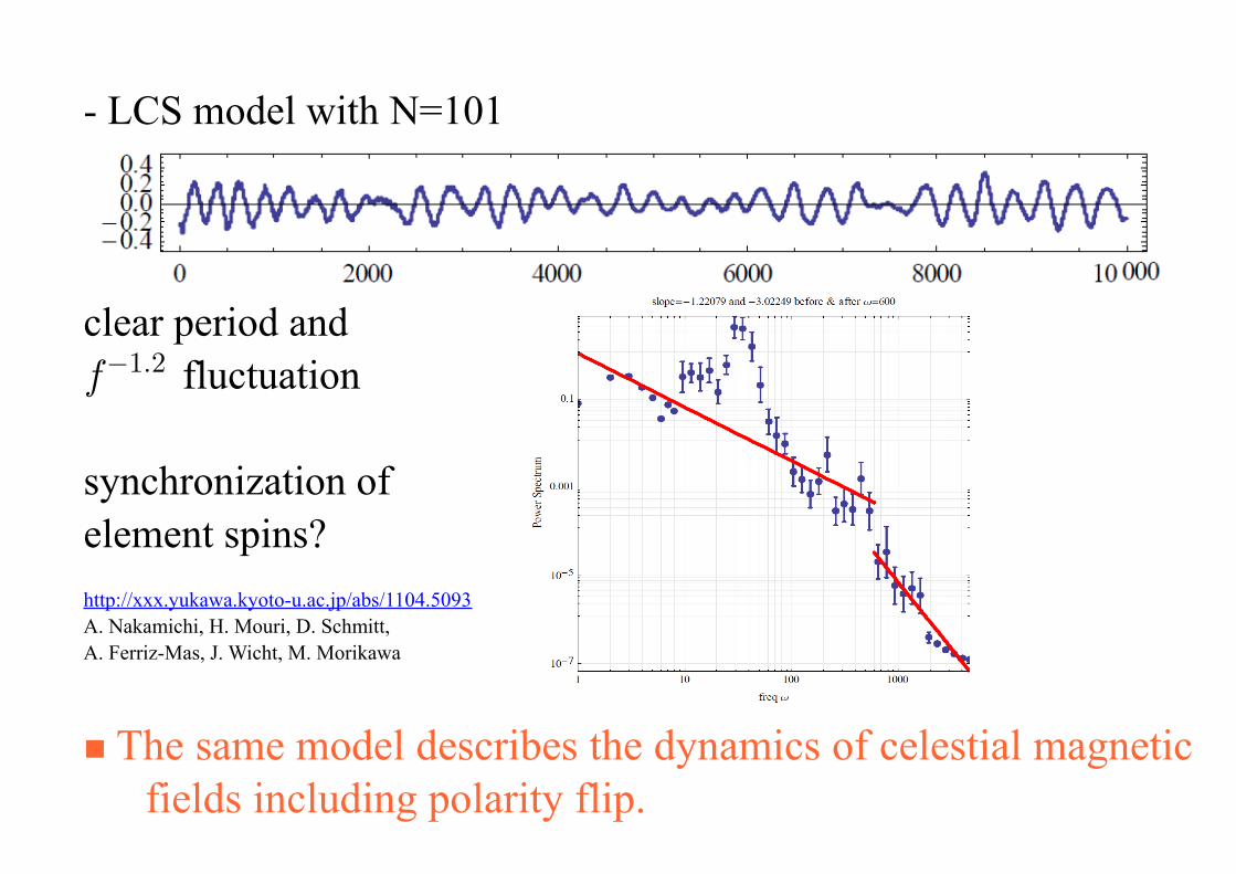
■ x triggers SSB initially 0S B× >r r

⇒ linear bias ⇒ force j toward

0j+ >

■ mixed→pure

in the factor ( ) ( )[ ]/exp t B kTa bmj= -h , the effective temperature

( )/T tj →0 ⇒spin is brought into a pure state↑

■ positive feedback linear bias is enhanced furthr ⇒ spin Sr

tends to be

more parallel to Br

.

- This positive feedback fixes the spin ↑, order variable j j+® .

4 2 0 2 4

210

1

2

3

V

j+j-

­

■ On the other hand if initially 0S B× <r r

, then the above process

fixes the spin↓, order variable j-.

■ results: we solved the coupled equations for r and j .

If ( )1 0

00 0

ræ ö÷ç ÷= ç ÷ç ÷çè ø

, then

If ( )0 0

00 1

ræ ö÷ç ÷= ç ÷ç ÷çè ø

, then

Further,

If ( )0.4 0.49

00.49 0.6

ræ ö÷ç ÷= ç ÷ç ÷çè ø

etc.

then, the frequency distribution

yields QM results( ) ( ) ( )2Trt t tj r r

- comments

1. `world bifurcation`(many world)→`SSB`(our world)

2. For the general initial condition a b­ + ¯ , bias ( )/ S Bd m g= ×r r

affects ( ),P tj non-linearly.

a faithful measurement needs a calibration.

3. a relevant time scale: 1

20

1ln

2

gt

ed

g g g

-é æ öù÷ç= +ê ú÷ç ÷è øê úë û

i.e. the completion time needed for SSB.

4. Application to various measurement

processes are possible.

§5 EPR measurement (two spins 1 2,S Sr r

)

( )2

2 2 41

2 2 4!

(bath)

m

S

L

B

m

mf

lf f f= ¶ - -

+ +×r r

- spatially separated spins

- localized apparatus 1 2,f f measure

each spin under individual

magnetic fields 1 2,B B .

are applied

- only causal interaction

- initial state of the system measured:

-6 -4 -2 0 2 4 6

-20

-15

-10

-5

0

5

V

1j j+®-6 -4 -2 0 2 4 6

-20

-15

-10

-5

0

5

V

2j j-®

2x vt= - 1x vt=

1Sr

1j2j

2Sr

t

x

1B2B

( )1 2 1 2

1

2y = ­ Ä ¯ - ¯ Ä ­

- Correlation terms in generalized effective action

( ) ( ) ( )x S x B x dxmf ×òr r

→ ( )( )Tr S B x dxmj r ×òr r

( ) ( )1 2x x

S B S Bmf mf× ×òò) )r r r r) )

→ ( ) ( ) ( ) ( )( ) ( ) ( )21 1 1 2 2 2Tri i j ji x B x S x S x B x xm j r jòò

) )

...yields stochastic diff. Eequations:

( )

( )

31 1 1 1 1 1 1

32 2 2 2 2 2 2

Tr3!

Tr3!

S B B

S B B

lj gj j m r x

lj gj j m r x

= - + × + ×

= - + × + ×

r r r r&

r r r r&

1 2i jx x ← ( ) ( )( )1 2ˆ ˆi jTr S Sr ( ijd- intially, quantum corelation)

For the state 1 2r r rº Ä

( ) ( )[ ] ( )[ ]

( )[ ]

3

3 3

[ , ] , ,

, . .

di S t a S t S b S t S

dt

c S t S h c

rw r r r

r

+ - - += - + +

+ +

- From the initial state ( )1 2 1 2

1

2y = ­ Ä ¯ - ¯ Ä ­ ,

1 2{ (0,0,1), (0,0,1)}B B= =r r

or

1 2{ (1,0,0), (1,0,0)}B B= =r r

etc. complete anti-correlation is

obtained.

Spin state r and meter read j are consistent with each other.

■ Bell in-equallity is violated?

- in probability ( ) ( )1 2 1 1 2 2( , ) , ,final finalP B B B B dj l j l r l= ò the

weight r depends on 1 1 2 2, , ,B Bj j . Therefore this is not the `hidden

variable theory`.

- 1 2i jx x ← ( ) ( )( )1 2ˆ ˆi jTr S Sr all the correlations of quantum theory is

included.

- Evolutions of the classical field j and the density matrix r couple

with each other. Positive feedback is the essence.

- Actually

( ) 1/21 1 / , 2B td x g e g-= × »r r

(g :friction M. Suzuki, Adv. Chem. Phys. 46 (1981), 195.) and

( ) ( ) ( ) ( )1 21 2P B P B P+ - +-=r r

yield

( ) ( )

( ) ( )1 2

1/2 1/21 1 2 2

11 2

,

erf erf

C B B P P P P

B B

B B

g x g x

g

++ -- +- -+

- -

-

º + - +

= × ×

» - ×

r r

r r r r

r r

.

Setting the magnetic field 1 2B B g=r r

makes ( )1 2 12, cosC B B q» -r r

.

Thus if the `accuracy` ( ( )erf , ,...g ) are sufficient, we have

( ) ( ) ( ) ( )1 2 1 2 1 2 1 2, , , , 2C B B C B B C B B C B B¢ ¢ ¢ ¢+ + - >r r r r r r r r

■ There is a possibility that the Bell inequality is violated.

§6 Origin of the primordial density fluctuations

■ The inflationary model in the early Universe

- The scenario:

from FRW expansion（ ( )a t tµ ）

then, de Sitter expansion（ ( ) Hta t eµ ）

connected to FRW（ ( )a t tµ ）

- Inflaton field (scalar field) promotes the

inflation

- k-mode obeys ( )22 22 0kt

kHv k H e v¢¢ + - =

and highly squeezes, yielding IR-fluctuations.

( )1/2 11kHtv k ik eH- -» + （ k kv ajº ）

t_f

tt

スケール

t_f t_nowt_i

■ Universal inflation model?

A standard model but allows

negative region of the

potential. Then, this model

always enters into the period

of stagflation ( 0Hf fr r= = =& but j ® ¥), where the expansion

stops. Then the uniform mode 0j becomes unstable and decays →

FRuniverse

⇒L-self regulation Phys.Rev.D80:063520,2009

( )V f

f

( )V f

f

( )V f

f

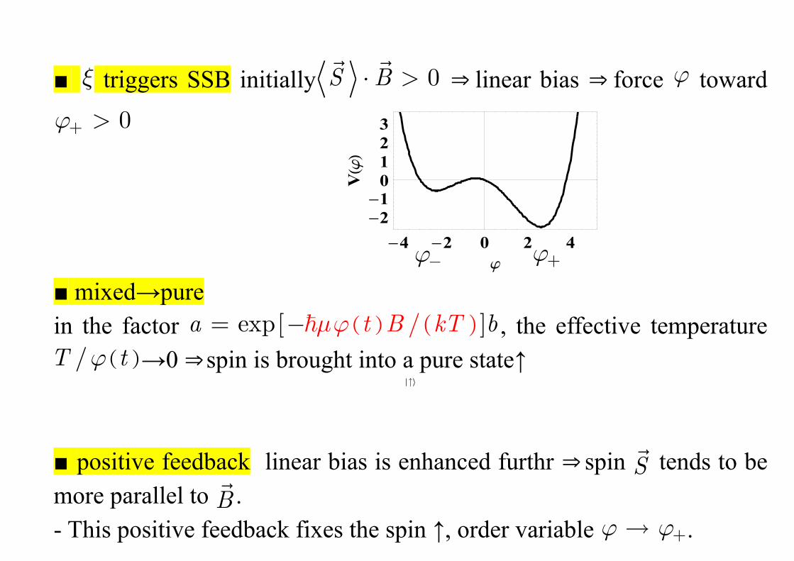
■ standard theory assumes

( ) ( ) ( ) 2

. .

ˆ ˆk

clasicalquantum theory

stat mech

x y kf f dj=144424443144444424444443

, k

k

v

aj º

i.e. a mode becomes classical when goes beyond the horizon.

Therefore ( ) ( ) ( )

23 2

3 / 0

4

22k

k aH

k v HP

adj

ppp ®= ¾¾¾¾¾® (scale invariant)

each mode evolves analogously

→ scale invariant fluctuations

l_0

1/H

t

t_1 t_2

k_1 k_2

■ quantum → classical fluctuation: analogous to EPR measurement

de Sitterexpansion

horizon size (causal limit)

squeezed state (after complete measurement)

If at 1x , then at 2x or,

If at 1x , then at 2x

■ Interaction in the Universe at reheating stage.

case of spin

interaction 4lf , 0f j dj= +the term ( )2

0 kj dj ( )20 kj dj yields

( ) ( ) ( ) ( )2 20 0 0 k dkx yk fl fj dj lj jG = G + -ò% % % % % %% %

SBm jr r

20k klf j j

-6 -4 -2 0 2 4 6

-20

-15

-10

-5

0

5

V

( ) ( ) ( )3 3

320

sin[ ]

34Re 0

kzdk O k

zz

h hh hp

f f¥ éæ ö ù¢ - ÷çê ú= +÷ç ÷ç ¢ê úè øë ûò

r

...IR( 0k ® ) converges → retG : mechanics

( ) ( )( )

2

20 2

1 1si ]

m 2In[

04

kz kdz

z k

O k

h hhhh h

pf f

¥¢é ùæ ö- ÷ç- +ê ú÷ç ÷ç ¢¢ è øê ú= ê ú

ê ú+ë û

òr

… IR-divergent → cG : statistical mech.

yields scale free fluctuations

■ Applying the least action method onReG% , (not ImG% , stat. mech. )

( ) ( )( ) ( ) ( ) ( )retxt

x V x dyG x y y xj j j x-¥

¢= - + - +òW

where ( ) ( ) ( ) ( ) ( )22 2c 0 0x y G x y x yx x l j j= -

IR-divergent statistical fluctuations

Leaving the most relevant part k kj x»&& , we have

( ) ( ) ( ) ( )23 42 2

03 / 1

4

22k k aH

k HP tdj

pj l j

pp == ¾¾¾¾¾® D

i.e. scale invariance is universal but the amplitude is not

present case, setting ( )0 0 0/ , 0t Vj j jD » »& yield ( )( )2

12

HP Odj p=

chaotic 4lf model ( 0 0j » ) yields no fluctuations

In general, the amplitude depends on the interaction at reheating

■ quantum theory in the inflationary era

- correlation in the quantum system ( )ˆ xf is traced in the macroscopic

pattern in apparatus ( ),t xjr

. This evolves into the present large scale

structure.

i.e. the quantum system ( )ˆ xf disappears and only apparatus remains in

the universe.

- IR-divergence in Re Im,G G : does it factorize? ...not solved

[ ] ( ) ( )e ImR1exp exp

2Z J i L J G G J

i J

dd

é ù é ù= +ê ú ê úë ûë ûò ò

- variety of reheating mechanism → selection of the inflation models

§7 summary

1．We constructed a physical quantum measurement model.

- phase transition (SSB), de/pro coherence, positive feedback

- measurement process is a phase transition (SSB)

it is deterministic ( V ¢- ) as well as non-determinsitic( ( ),t xxr

)

- EPR measurement process, Bell inequality

2． Origin of the primordial density fluctuations

- classical apparatus variable determines the large scale structure

- statistical fluctuations are autonomously generated as in the

case of EPR measurement.

- density fluctuations depends on the reheating interaction and

the potential

■ Cosmological structures are not separated with each other but micro-

macro hierarchy are connected:

measurement process,

EPR,

celestial magnetism,

primordial density fluctuations

...

- A system can be non-equilibrium and dissipative at any scale.