MEASUREMENT AND ANALYSIS OF MID WAVELENGTH RAIL IRREGULARITY

Prof. A. Bracciali, Dr. F. Piccioli, T. De Cicco

Dipartimento di Meccanica e Tecnologie Industriali Università di Firenze, via Santa Marta 3, 50139 Firenze

andrea.bracciali@unifi.it, fabio.piccioli@unifi.it, teo.decicco@gmail.com KEYWORDS: Railhead irregularity, groundborne vibrations, mid wavelength ABSTRACT Groundborne vibrations are becoming more and more important as train speed increases. Longer wavelength rail and track defects are excited at such velocities and lead to potentially unacceptable annoyance also at long distances from the railway line. The paper critically compares European Standards currently in force on rail irregularity measurements and describes the results obtained extending the range of a trolley typically used only for short wavelengths assessment (related to noise). The practical possibility to measure comfortably wavelengths up to 3 m will be shown. INTRODUCTION Rail irregularities in the longitudinal (vertical) direction are responsible for abnormal wheel rail excitation forces that ultimately lead to higher vibration and noise, passenger discomfort, high stress in structural components. The assessment of the rail irregularity is normally related to the maintenance technique that is used to remove the defect: wavelengths shorter than one metre are measured by portable instruments on unloaded track and removed by grinding while wavelengths longer than three metres are measured by measuring coaches (i.e. with laden track) and corrected by track tamping. The missing range of wavelengths, i.e. one to three metres, in nevertheless extremely important for groundborne vibration generation, especially with the general tendency to increase train speed. A simple calculation shows that a train running at 360 km/h on a 3 m irregularity produces a 33.3 Hz excitation that can be easily transmitted through the ground disturbing the population even on pretty long distances depending on the nature of the soil. The measurement of rail irregularity in the mid wavelength range has been faced by properly modifying the measuring procedures related to the use of a trolley normally used for the assessment of rail longitudinal defects for acoustic purposes. The results will be shown for three different measuring campaigns, including the results from a preliminary test and calibration phase. The data obtained during these campaigns are expected to be used as input for numerical models development and validation. RAILHEAD IRREGULARITY SEEN AS SURFACE DEFECT Wheel-rail interaction is responsible for noise and vibration generation. The contact stiffness, typically in the order of 1 GN/m, leads to high dynamic forces in the high frequency domain. The most widely accepted model for noise generation (the computer code TWINS), consider as a fundamental input the railhead longitudinal (vertical) profile [1]. Recent standards on noise type testing of vehicles include the measurement of that rail characteristics [2, 3] in a rather short wavelength range. The lower limit of the wavelength range is defined by the so-called contact patch filter, as wheel and rail have approximately the same stiffness being made of materials (steels) with the same Young’s modulus, resulting in a finite and non-negligible contact area that “filters out” all the components shorter than approximately 1 cm.

The upper limit of the wavelength range is defined by both the field of interest and the measuring technology. Following the fundamental law of any wave phenomenon, i.e. v=λ f where f is the frequency, λ is the wavelength [m] and v is the speed [m/s], the noise generation at the lower frequency limit and the maximum considered speed gives the longest wavelength. By using typical parameters of noise disturbance, i.e. a frequency of around 200 Hz and a speed of 180 km/h (=50 m/s), this results in a wavelength of λ = v/f=50/200=0.25 m. This wavelength was considered also in the so-called “road test” [4] of the more recent standards on the railhead irregularity measurements for test site assessment [5]. It was found that this wavelength can be considered as the upper limit for equipment with fixed-length capabilities; it was moreover found, although this was not the main reason for the road test, that all the equipment that participated to the test gave a reasonably fair and repeatable estimation of rail roughness under well specified conditions [4]. The description and the comparison of the equipment lies beyond the scope of this paper; the reader is referred to [1]. TRACK IRREGULARITY SEEN AS GEOMETRY DEFECT It is known that the conflict between guidance offered by tapered wheel profiles mounted on rigid wheelsets and vehicle stability can generate an undesired and potentially very dangerous parasitic motion, named “hunting”, that may lead to derailments. Hunting, i.e. an oscillatory motion around the vertical axis of the bogie, happens especially at high speed if the equivalent conicity is high and the damping of the bogie is low. Vehicles designed to have a stable run at high speeds are normally equipped with long base bogies, high wheelset yaw stiffness and anti-yaw dampers fitted between the bogie frame and the carbody to minimize the risk of hunting. Although hunting may happen even on a perfect track, track irregularity is nevertheless considered an important “triggering” and excitation source to rolling stock dynamics especially on ballasted track. Ballast is still the standard for the track formation in many countries in the world (including China, Russia, France, Italy, Spain), while slab track has been used to a somewhat large extent only in Germany. Ballast is a “live” matter that may require frequent profiling, tamping and renewal, depending on a number of parameters that are beyond the scope of this paper. For sure, ballastless (or slab) track virtually eliminates time-dependent degradation of the railway superstructure, this being the main reason for applying a so high cost track formation. Any track section on a vertical plane can be fully defined by four independent parameters, i.e. cross level (cant or superelevation), gauge, alignment and longitudinal level [6]. The first two parameters can be managed virtually tamping the single sleeper, the others are relative to the position of the line on a global measuring system (i.e. they represent the track centreline in the y-lateral and z-vertical coordinate respectively) and must be managed by track maintenance machines. The effect of alignment and longitudinal defects on the vehicle dynamic behaviour level is normally weakly coupled, in the sense that alignment is normally responsible for abnormally high lateral response of the vehicle while longitudinal level is responsible for vertical excitation and movements of the train and the track. Limiting the discussion only to vertical irregularity, modern passenger vehicles are built with rather soft secondary suspension that limit the effect on the passengers. The same thing is not possible in the lateral direction, where vehicle gauge must be respected using bumpstops in extreme cases. As a result, travelling on modern trains running over modern lines results mainly in a lateral passenger discomfort. Incidentally, this is exactly the opposite of road vehicles, where lateral stiffness is low (drivers can often “adjust” somewhat the trajectory to local conditions) and vertical road irregularity may be high (depending on the terrain --- or on the maintenance conditions of the road surface!).

Whenever an engineering “problem” occurs, it is worth to define a physical quantity describing it, including the definition of the measuring techniques, and the possible remedies. About track irregularities, they can only be measured by a trolley or, in modern times, by a measuring train due to the long distances intrinsic in the measurement. This incidentally implies that track irregularities are measured with the track loaded by the measuring train, a condition that is certainly preferable. The European Standard [6] defines three fields of wavelengths, named D1 (3<λ≤25 m), D2 (25<λ≤70 m) and D3 (70<λ≤150 m), where the last should be “used for measuring long wavelength defects. Generally this range should only be considered for line speeds greater than 250 km/h”. By using again the law of wave phenomena, the shortest wavelength of λ=3 m when travelling at 250 km/h (=69.44 m/s) leads to a maximum frequency of f =v/λ=69.44/3=23 Hz. On the other side, considering also the railhead irregularity as a source of disturbance, and limiting the measuring field to the longest wavelength of λ=0.25 m as described above and reported in [2], for a train running at 250 km/h leads to leads to a minimum frequency of f =v/λ=69.44/0.25=278 Hz. It is clear from this example that for a train running at 250 km/h there is a “hole” in the standardization measurements and limits in the excitation frequency range 23.1÷278 Hz (Figure 1). Similar frequency ranges can readily be obtained by changing the train speed, but for high speed train a large portion of the spectrum responsible for groundborne vibrations is neglected.

Figure 1. Wavelength of defects and corresponding frequencies at 250 km/h.

The main reason for this lack of the definition in the wavelength range 0.25<λ<3 m is that shorter wavelength defects can be corrected by rail grinding while longer wavelength defects can be corrected by track tamping. The measuring technologies are also dramatically different, talking in terms of microns (or sub-microns) for railhead irregularities in the short-wavelength domain (λ<0.25 m, the so-called “rail roughness”) and in terms of mm for railhead irregularities in the long-wavelength domain (λ>3 m). Precision and repeatability must be properly assessed. While it appears quite clear that measuring coaches can hardly extend their field of investigations to shorter wavelengths for under range problems of the measuring chain, it appears possible in principle to extend the capabilities of some “rail roughness measuring equipment” provided that overloads are not encountered due to expectedly higher defect amplitudes. TYPICAL RAIL AND TRACK DEFECT SPECTRA The definition of the limit spectra in the standards reflects the average status of track in “normal” service. It is quite hard to define what is “normal”, as railway practice differs considerably between different member states of the EU and traffic tends to be either heterogeneous (on older lines) or absolutely separated (for example freight trains can not run on high speed lines in France due to 3.5% gradient). EN ISO 3095:2005 [2], which is related to external noise measurements during type testing of rolling stock, defines a limit spectrum which is defined on a number of considerations (measurements and calculations, described in Annex C) starting from the “roughness of typically good European rails”. Whatever the calculation scheme is, it is apparent that the energy content (spectra are defined as RMS

Wavelenghts in [m] 0.01 0.1 1 10 100

EN 13848-1 EN ISO 3095 + TSI

0.25 3 75

Frequency [Hz] at 250 km/h 6950 278 23.1 0.92 ?

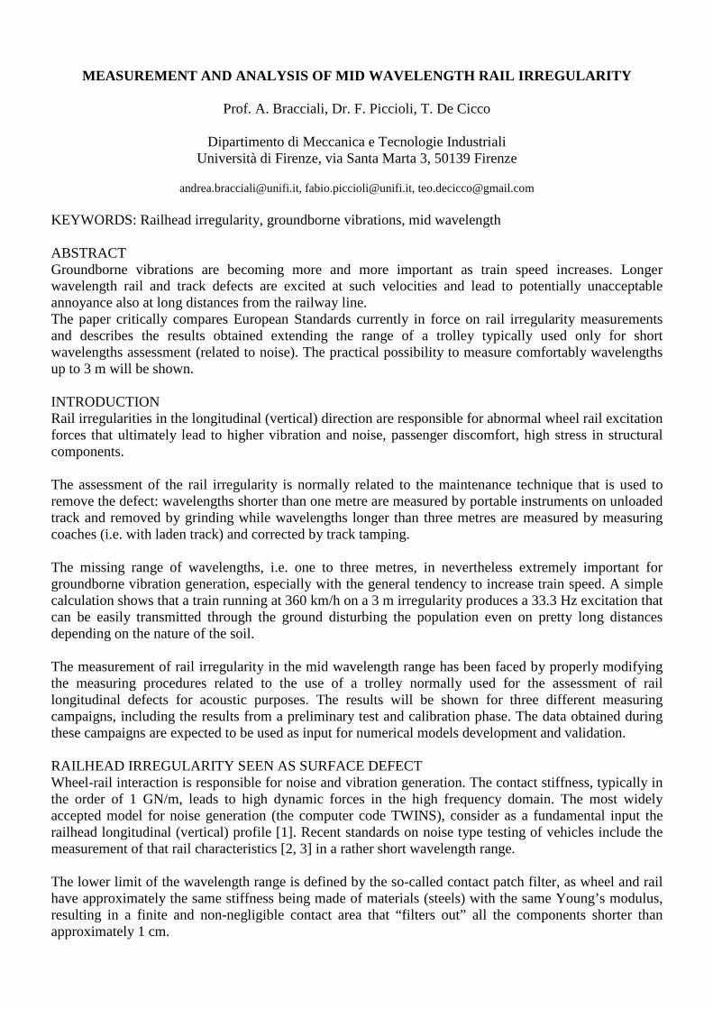
values expressed in dB ref. 1 µm) at the lower frequencies (i.e. longer wavelengths) increases despite the fact the bandwidth is smaller there (Figure 2).

Figure 2. One-third octave band roughness spectrum of typical European good rails (the upper

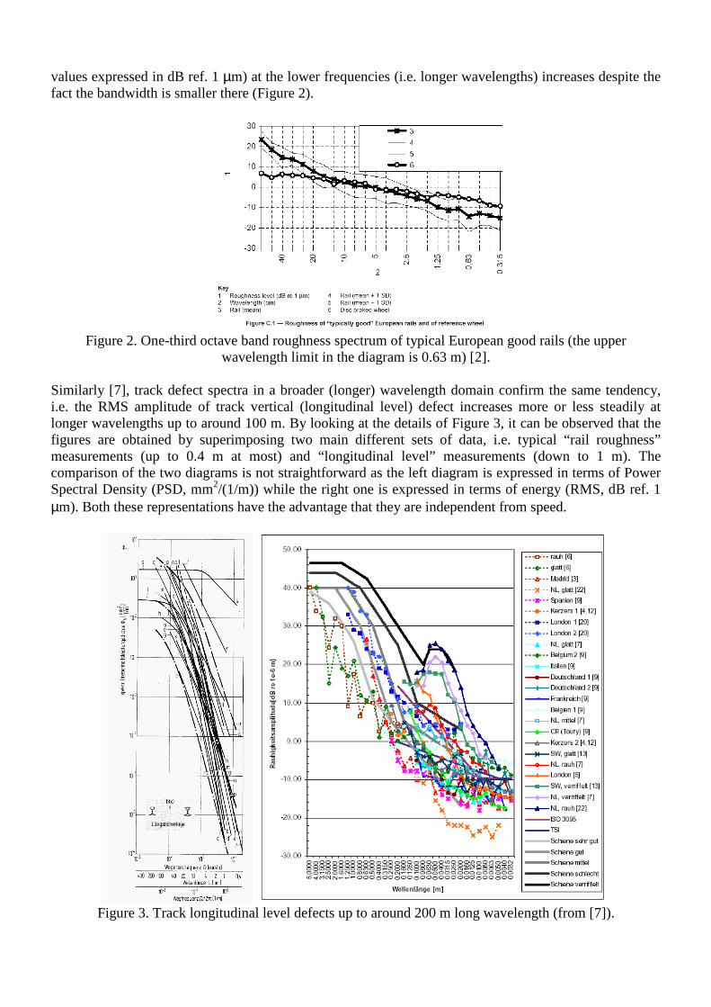
wavelength limit in the diagram is 0.63 m) [2]. Similarly [7], track defect spectra in a broader (longer) wavelength domain confirm the same tendency, i.e. the RMS amplitude of track vertical (longitudinal level) defect increases more or less steadily at longer wavelengths up to around 100 m. By looking at the details of Figure 3, it can be observed that the figures are obtained by superimposing two main different sets of data, i.e. typical “rail roughness” measurements (up to 0.4 m at most) and “longitudinal level” measurements (down to 1 m). The comparison of the two diagrams is not straightforward as the left diagram is expressed in terms of Power Spectral Density (PSD, mm2/(1/m)) while the right one is expressed in terms of energy (RMS, dB ref. 1 µm). Both these representations have the advantage that they are independent from speed.

Figure 3. Track longitudinal level defects up to around 200 m long wavelength (from [7]).

MEASURING DEVICE DESCRIPTION To face the problem of the quantification of rail longitudinal defect in the mid-wavelength (1÷3 m) domain, the equipment named “Corrugation Analysis Trolley” (CAT), a trolley manufactured by RailMeasurement Ltd. [8] was used. The version used in this activity (CAT Type 1) is sensibly different from the mechanical point of view with the version currently marketed but the physical principle on which it is based remains unchanged and still holds. It is made of an aluminium frame including a 12 mm-diameter hardened steel ball sliding over the rail that is connected to a servoaccelerometer. The sensor is decoupled from the vertical movements of the trolley frame by means of an ultra-low stiffness leaf spring. The accelerometer signal is integrated first in an analogue circuitry on the trolley and then the velocity signal is digitised by a PCMCIA card with an A/D converter. The second integration step, supplying the displacement, is performed by the software. A digital encoder connected to a wheel rotating in contact with the rail via a rubber O-ring acts as an odometer. The output of the measurement is the sampled vertical profile of the railhead measured along the longitudinal profile identified by the lateral position of the sliding ball. Sampling distance may be selected as 1 or 2 mm; the best resolution was used throughout all this activity. It must be said that the while CAT was originally designed for regular rail corrugation check and trackworks quality issues (grinding acceptance), where amplitudes can be of several hundred µm, through the years it proved its reliability also for different purposes. It is now routinely used for noise-related measurements, a field where the amplitudes can be markedly lower (<1 µm). The use as a measuring equipment for long wavelengths up to 3 m was new for the author, requiring an accurate and time consuming testing phase changing all the parameters of the instruments until the best results were obtained. Being an inertial device requiring a double integration of the acquired signal, the CAT potentially suffers of drift problems due to even infinitesimal offset of the signal. Is therefore necessary to use an RC high-pass digital network to avoid this source of error. Being interested in long wavelengths, i.e. to phenomena with very low frequency, the only way to counteract the effect of the RC filter while at the same time avoiding drift is to walk as fast as possible. As a drawback, running fast leads to stronger impacts with local irregularities, possibly affecting more the results of the measurements. In all the tests described in this paper the walking speed was kept at 2 m/s ± 20% (i.e. in the range 1.6÷2.4 m/s). This speed was selected, after numerous tests on different track formations (ballast with monobloc and bibloc sleepers, slab track) as the maximum speed that can be sustained for pretty long distances (several hundred meters) under unfavourable (very hot) meteorological conditions (Figure 4).

Figure 4. Snapshot taken while pushing the trolley at around at 2 m/s, the maximum safe speed that can

be sustained on a ballasted track with bi-bloc sleepers.

MEASURING ACTIVITIES During the activities described in the aforementioned “road test” [4], it was found that, at extra-low amplitudes, even small local irregularities may lead to unacceptable contaminations of the results for noise-related rail roughness measurements. It was therefore recommended to thoroughly clean the railhead before taking the measurements. This procedure was found to be inapplicable for the activity described in this paper as the measuring length is some hundred meters and there is not normally time enough to clean the rails satisfactorily. Track possession may be limited to just a couple of hours, typically during the night on high speed lines, with related visibility problems. While the selection of the measuring site can avoid to some extent the presence of (insulated) rail joints, being the track mostly made of continuously welded rails, many local irregularities (ballast prints, wheelburns, dried bird droppings) are normally observed during the measuring site survey. No attempt is normally made to take note of their position as: • they are in practice unavoidable (it is impossible to find a lateral position of the sensor that does not

include any of these defects); • they will stay on the rail at least until the next grinding and therefore any major disturbance to the

acquired signals can be traced back with a supplementary visit to the track; • during the night it is too dark to even forecast this activity with the normally restricted available time.

Figure 5. Ballast print (left) and dried bird droppings (right): typical defects of outside track in country areas.

The individuation of the running band is normally pretty easy on tangent track. On gently curved track, with the large radii typical of high speed lines, sometimes two distinct running bands of variable amplitude and position were identified on the low rail. Asymmetric grinding and mixed rolling stock may generate distinct running bands. It is believed that the low frequency (long wavelengths) content of these running bands is approximately the same. In this paper we report the results of measuring campaigns performed in 2008 in three different sites, two on high speed lines and one on a conventional line. In all these situations the measurement of a 200 m-long track section was requested on both rails. For reasons that will be apparent in the next chapters, the actual measurement length was 240 m each time. In one case the entire measuring activity (i.e. the actual track possession) was limited to less than one hour, comprising three measurements per rail. Equipment set-up was done just before the measurements start. The CAT takes power supply from a USB port of the connected laptop (note: this modification being made by one of the authors); modern laptop ensure a continuous operation of the equipment up to around 4 hours before needing a battery change.

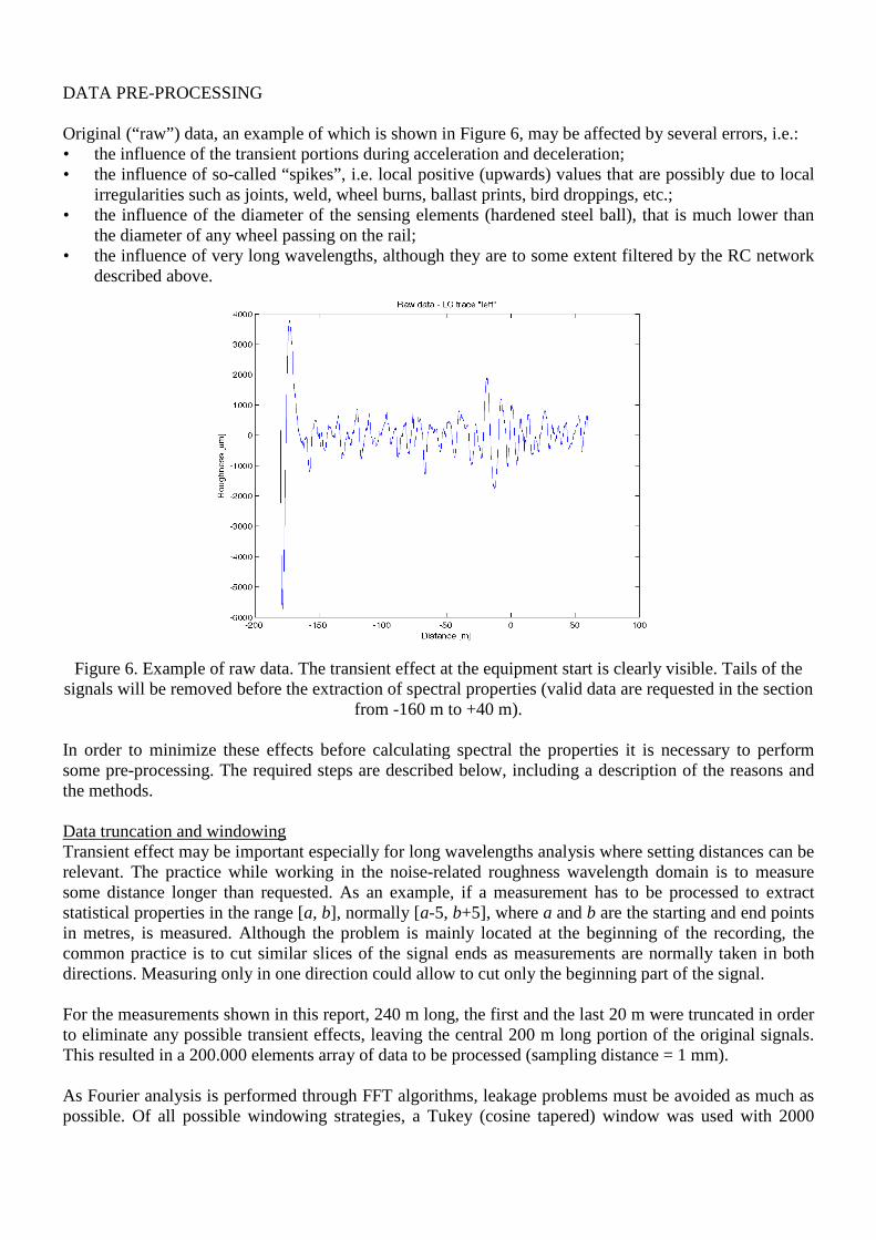
DATA PRE-PROCESSING Original (“raw”) data, an example of which is shown in Figure 6, may be affected by several errors, i.e.: • the influence of the transient portions during acceleration and deceleration; • the influence of so-called “spikes”, i.e. local positive (upwards) values that are possibly due to local

irregularities such as joints, weld, wheel burns, ballast prints, bird droppings, etc.; • the influence of the diameter of the sensing elements (hardened steel ball), that is much lower than

the diameter of any wheel passing on the rail; • the influence of very long wavelengths, although they are to some extent filtered by the RC network

described above.

Figure 6. Example of raw data. The transient effect at the equipment start is clearly visible. Tails of the

signals will be removed before the extraction of spectral properties (valid data are requested in the section from -160 m to +40 m).

In order to minimize these effects before calculating spectral the properties it is necessary to perform some pre-processing. The required steps are described below, including a description of the reasons and the methods. Data truncation and windowing Transient effect may be important especially for long wavelengths analysis where setting distances can be relevant. The practice while working in the noise-related roughness wavelength domain is to measure some distance longer than requested. As an example, if a measurement has to be processed to extract statistical properties in the range [a, b], normally [a-5, b+5], where a and b are the starting and end points in metres, is measured. Although the problem is mainly located at the beginning of the recording, the common practice is to cut similar slices of the signal ends as measurements are normally taken in both directions. Measuring only in one direction could allow to cut only the beginning part of the signal. For the measurements shown in this report, 240 m long, the first and the last 20 m were truncated in order to eliminate any possible transient effects, leaving the central 200 m long portion of the original signals. This resulted in a 200.000 elements array of data to be processed (sampling distance = 1 mm). As Fourier analysis is performed through FFT algorithms, leakage problems must be avoided as much as possible. Of all possible windowing strategies, a Tukey (cosine tapered) window was used with 2000

elements (equivalent to 2 m) at each end. The effect on the energy of the signal is negligible (4/200= 0.02 = -34 dB) and therefore it was decided not to perform any correction on it. Spike removal There is a large concern in the scientific community about the contamination that local defects may introduce in the measurements generating the so-called “spikes” in the data sequence. In this chapter we will prove that this type of defects are not influent on the quality of the data in the longer 1 to 3 m wavelength range. Some preliminary analysis can be done on the field by using the CAT’s software. The experience gained after years of use of the CAT instructs to check the existence of peaks by looking at low-range wavelengths (i.e. higher frequencies). As a rule of thumb, the 30÷100 mm wavelength range (one of the pre-set available ranges) appears to be the best candidate to identify peaks.

Figure 7. Spikes of different genesis on some measurements. “Random” spikes (top left), grinding generated spikes (top right), rail welds generated spikes (bottom left), a mixture o the three (bottom right).

All the diagrams are the superposition of two measurements, showing the repeatability of the data.

As a manual spike removal process is complicated and not standardized, the spike removal processing was done by using the standardized routine that and can be found in [5]. Figure 8 shows the effect of spike removal on a high-pass filtered signal. Correctly, all the removed components are negative (spikes are upwards). The effect on the spectral distribution looks anyway important for wavelengths λ<7 mm. Apparently, spikes are in this case unable to affect sensibly the measurements in the range of interest of this paper (1 to 3 m).

Figure 8. Spike removal in a high-pass filtered data sequence. Signal removed by the spike removal procedure (top); estimate of the transfer function between sequences before and after spike removal

(bottom). Frequency is evaluated for a 1000 samples/s sampling frequency (equivalent to 1 m/s speed). The frequency of 142 Hz is therefore equivalent to 1000/142=7 mm wavelength.

A similar behaviour was observed on all the recorded signals, reinforcing the deduction that the spike processing procedure in its present form is needed only for acoustic processing where wavelength in the order of 1 cm is important, while for long wavelengths investigations this step is not necessary. A similar conclusion can be reached through a more general evaluation of the effect of spikes on spectral estimation that can be done by using the perfect filtering procedure described later. Generally speaking, ideal peaks (Dirac’s delta) have the same energy content in the entire frequency domain (i.e. a flat spectrum in narrow band representation). Changing to constant percentage band spectrum, as the one-third octave bandwidth decreases with increasing wavelength (i.e. decreasing frequency), the shape of the RMS spectrum of a single 100 µm peak in a 10.000 zero-elements array is “increasing” towards shorter wavelengths (Figure 9) . The effect on each one-third octave band is shown in Figure 10, from which it is clear that the mentioned peak has an influence that reduces by approximately a factor 250 from the one-third octave band centred at λ=0.010 m (r=5 µm) to the one-third octave band centred at λ=3.150 m (r=0.02 µm) The effect of the peaks will be therefore higher on shorter wavelengths, affecting less longer wavelengths that are characterized by higher amplitudes on actual tracks as described above. For the purposes of the present work, the effect of the peaks is negligible on the long wavelengths considered. Spike removal confirms to be unnecessary and irrelevant at longer wavelengths. In any case, as the calculation effort is not excessive, it was done on all signals.

Figure 9. RMS spectrum of a single peak 100 µm high in a 10.000 zero-elements array compared to TSI

(green) and EN ISO 3095:2005 roughness limits.

Figure 10. One-third octave analysis performed with the perfect filtering technique of a single peak

100 µm high in a 10.000 zero-elements array. Curvature processing A curvature processing algorithm is described in prEN15610 [5]. Although this curvature removes mainly the high frequency (i.e. the short wavelengths) content, it is anyway useful to remove “background noise” in the data and complements well the spike removal procedure, virtually eliminating any residual pit remaining. Figure 11 shows the effects of the curvature processing procedure, with removed component mainly positive (troughs downwards). For this example the effect is almost insensible up to f=10Hz, i.e. λ=0.1 m. As supposed, also this effect is negligible in the present activity.

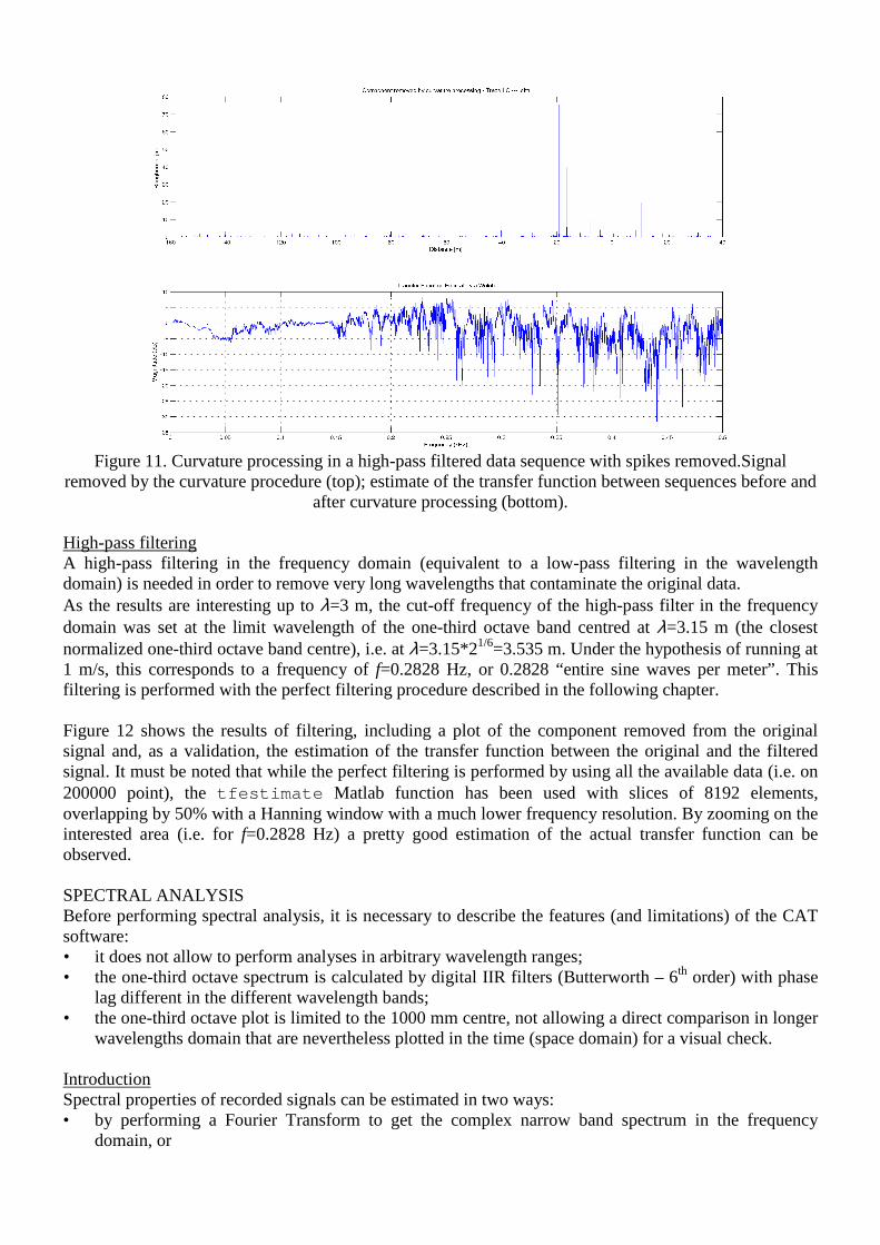
Figure 11. Curvature processing in a high-pass filtered data sequence with spikes removed.Signal

removed by the curvature procedure (top); estimate of the transfer function between sequences before and after curvature processing (bottom).

High-pass filtering A high-pass filtering in the frequency domain (equivalent to a low-pass filtering in the wavelength domain) is needed in order to remove very long wavelengths that contaminate the original data. As the results are interesting up to λ=3 m, the cut-off frequency of the high-pass filter in the frequency domain was set at the limit wavelength of the one-third octave band centred at λ=3.15 m (the closest normalized one-third octave band centre), i.e. at λ=3.15*21/6=3.535 m. Under the hypothesis of running at 1 m/s, this corresponds to a frequency of f=0.2828 Hz, or 0.2828 “entire sine waves per meter”. This filtering is performed with the perfect filtering procedure described in the following chapter. Figure 12 shows the results of filtering, including a plot of the component removed from the original signal and, as a validation, the estimation of the transfer function between the original and the filtered signal. It must be noted that while the perfect filtering is performed by using all the available data (i.e. on 200000 point), the tfestimate Matlab function has been used with slices of 8192 elements, overlapping by 50% with a Hanning window with a much lower frequency resolution. By zooming on the interested area (i.e. for f=0.2828 Hz) a pretty good estimation of the actual transfer function can be observed. SPECTRAL ANALYSIS Before performing spectral analysis, it is necessary to describe the features (and limitations) of the CAT software: • it does not allow to perform analyses in arbitrary wavelength ranges; • the one-third octave spectrum is calculated by digital IIR filters (Butterworth – 6th order) with phase

lag different in the different wavelength bands; • the one-third octave plot is limited to the 1000 mm centre, not allowing a direct comparison in longer

wavelengths domain that are nevertheless plotted in the time (space domain) for a visual check. Introduction Spectral properties of recorded signals can be estimated in two ways: • by performing a Fourier Transform to get the complex narrow band spectrum in the frequency

domain, or

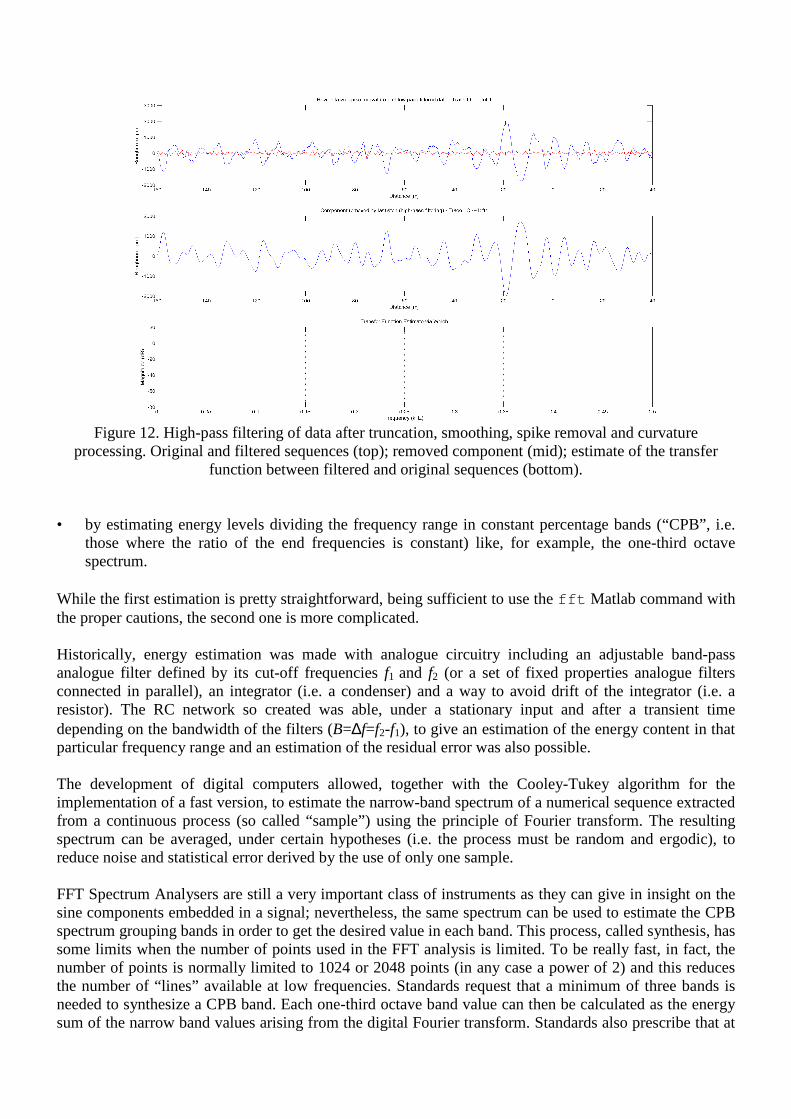
Figure 12. High-pass filtering of data after truncation, smoothing, spike removal and curvature

processing. Original and filtered sequences (top); removed component (mid); estimate of the transfer function between filtered and original sequences (bottom).

• by estimating energy levels dividing the frequency range in constant percentage bands (“CPB”, i.e.

those where the ratio of the end frequencies is constant) like, for example, the one-third octave spectrum.

While the first estimation is pretty straightforward, being sufficient to use the fft Matlab command with the proper cautions, the second one is more complicated. Historically, energy estimation was made with analogue circuitry including an adjustable band-pass analogue filter defined by its cut-off frequencies f1 and f2 (or a set of fixed properties analogue filters connected in parallel), an integrator (i.e. a condenser) and a way to avoid drift of the integrator (i.e. a resistor). The RC network so created was able, under a stationary input and after a transient time depending on the bandwidth of the filters (B=∆f=f2-f1), to give an estimation of the energy content in that particular frequency range and an estimation of the residual error was also possible. The development of digital computers allowed, together with the Cooley-Tukey algorithm for the implementation of a fast version, to estimate the narrow-band spectrum of a numerical sequence extracted from a continuous process (so called “sample”) using the principle of Fourier transform. The resulting spectrum can be averaged, under certain hypotheses (i.e. the process must be random and ergodic), to reduce noise and statistical error derived by the use of only one sample. FFT Spectrum Analysers are still a very important class of instruments as they can give in insight on the sine components embedded in a signal; nevertheless, the same spectrum can be used to estimate the CPB spectrum grouping bands in order to get the desired value in each band. This process, called synthesis, has some limits when the number of points used in the FFT analysis is limited. To be really fast, in fact, the number of points is normally limited to 1024 or 2048 points (in any case a power of 2) and this reduces the number of “lines” available at low frequencies. Standards request that a minimum of three bands is needed to synthesize a CPB band. Each one-third octave band value can then be calculated as the energy sum of the narrow band values arising from the digital Fourier transform. Standards also prescribe that at

the one-third octave band boundaries, this shall only take account of the portion of the narrow band, to which each value of the narrow band spectrum corresponds, that lies within the one-third octave band being evaluated. Digital Signal Processors, or DSP chips, can be used to simulate the behaviour of the analogue filters described above avoiding the problems of the FFT approach, i.e. performing in real time all the operations performed by an analogue set of parallel filters. This is, in fact, the typical construction of measuring instruments for acoustics where the use of CPB analysis is mandatory for physiological reasons of the human ear and perception. This class of instruments is not normally made to record long time histories but rather to record statistical indicators (spectra, Leq, LAmax, etc.) adjusting also typical noise properties (like the frequency weighting network or the time constant). Thanks to modern PC, the possibility to simulate via software the behaviour of the DSPs has become reality. Given an almost arbitrary long time history (comprising some million samples), it is possible to filter it and to obtain a high precision estimate of the spectral properties without the limitations of classical FFT analysers. The “perfect filtering technique” [9] approach was used in this work as the FFT algorithm is applied over the entire sequence, including therefore 200.000 samples. From the basic properties of digital sampling, it is known that frequency resolution only depends from the measuring time or, if preferred, by the ratio of the sampling frequency and the number of samples with the relationship df=1/T=fs/n. As the sampling of roughness measurements is 1 mm (fs=1000 Hz), it results in a df=1000/200000= 0.005 Hz. Although no synthesis is performed, FFT of a so long sequence would results in a high number of lines also for the longest wavelength (i.e. the smallest frequency) requested: n=∆f/df= (1/3.15*21/6 – 1/3.15/21/6) / 0.005= 14.7 = 14 lines. One-third octave spectra One-third band spectra are calculated by using the perfect filtering algorithm. Figure 13 and Figure 14 show the spectra calculated over the 200-metres long central portion of the signal. Limit curves from TSIs and EN ISO 3095 are linearly extrapolated (in a log-log domain) beyond their domain of definition.

Figure 13. One-third octave band roughness spectra of two different sites (a conventional speed line and a

high speed line) during the first measuring campaign.

Figure 14. One-third octave band roughness spectra of a high speed line during the second measuring

campaign.. DISCUSSION AND FURTHER DEVELOPMENTS Data collected extending to longer wavelengths the range of a trolley normally used for shorter wavelengths measurements appear to be consistent and repeatable. Running at 2 m/s resulted in good resolution at the longest one-third octave band centred at wavelength λ=3.15 m, while sensitivity at shorter wavelengths was much reduced (although of no interest in this case) as a possible combination of the curvature processing and a lower sensitivity of the equipment to this wavelengths at so high walking speeds. Nothing can be said about accuracy as there are neither standards to calibrate the equipment on these wavelength range nor available measurements made with a more precise instrument. Results are nevertheless in line with spectra found in the literature. A complete set of tools (spike removal, curvature processing, high-pass filtering, perfect filtering, estimation of RMS one-third octave band spectrum) were implemented with success. The calculation effort is limited and compatible with low-capabilities modern ultra-light laptops, needed for battery capacity and available working time. Further analyses will be conducted on the recorded signals as a first attempt revealed some interesting capabilities of the equipment up to and beyond wavelengths of around 10 m. CONCLUSIONS After a long tuning phase, operational and acquisition parameters for the measurements of the rail irregularity in the mid-wavelength domain (1 to 3 m) to be done with the CAT equipment were found. A satisfactory set of experimental and processing procedures gave repeatable estimation in this wavelength range opening a new field of application for the equipment which can be used for such purpose in all situations were groundborne vibrations are a major problem, including underground lines where frequencies are lower. The large experience gained and the convincing results are such that it looks like long wavelengths roughness measurements can be done fast and comfortably in most of the practical situations and railway environments. The use of the data for further processing and simulations (like groundborne vibration propagation) also looks possible with a high degree of reliability.

REFERENCES [1] D. Thompson, Railway Noise and Vibration - Mechanisms, Modelling and Means of Control,

Elsevier 2008, ISBN 9780080451473 [2] EN ISO 3095:2005, Railway applications - Acoustics - Measurement of noise emitted by railbound

vehicles, CEN, Brussels, 2005. [3] Commission Decision 2006/66/EC, Technical specification for interoperability relating to the

subsystem ‘rolling stock - noise’ of the trans-European conventional rail system, Official Journal of the European Union, 8.2.2006 and Commission Decision 2008/232/CE, Technical specification for interoperability relating to the ‘rolling stock’ sub-system of the trans-European high-speed rail system, Official Journal of the European Union, 26.3.2008.

[4] prCEN/TR 1-1:2008.2, Railway applications — Noise emission — Road test of draft standard for rail roughness measurement prEN 15610:2006, CEN, Brussels, 2008.

[5] prEN 15610:2006, Railway Application — Noise emission — Rail roughness measurement related to rolling noise generation, CEN, Brussels, 2006.

[6] EN 13848-1:2003+A1, Railway applications - Track - Track geometry quality - Part 1: Characterisation of track geometry, CEN, Brussels, 2008.

[7] R. Thornely-Taylor, W. Rücker, ISO/TC 108/SC 2/WG 8 N 210, Part (3) Measurements - Rail roughness measurements, May 2008.

[8] www.railmeasurement.com accessed on 10.04.2009. [9] A. Bracciali: Long roughness measurements – Analysis and possible protocol, 8th International

Workshop on Railway Noise, Buxton (UK), 7-11.9.2004 (on CD).