I

Measured GFR using a population

pharmacokinetic model for Iohexol

Kwame Boateng

Master’s thesis

Department of Pharmaceutical BioSciences

School of Pharmacy

Faculty of Mathematics and Natural Sciences

UNIVERSITETET I OSLO May 2016

II

III

Measured GFR using a population

pharmacokinetic model for Iohexol

Kwame Boateng

Master’s thesis

Department of Pharmaceutical BioSciences

School of Pharmacy

Faculty of Mathematics and Natural Sciences

UNIVERSITETET I OSLO May 2016

IV

® Kwame Boateng

Year 2016

MEASURED GFR USING A POPULATION PHARMACOKINETIC MODEL FOR

IOHEXOL

Kwame Boateng

http://www.duo.uio.no

Printed at Reprosentralen, Universitetet i Oslo

V

Abstract Introduction: Determining renal function (i.e glomerular filtration rate) is in many ways

essential in clinical practice, in terms of diagnosis and drug therapy. Exogenous markers,

such as iohexol, are mainly used for a more accurate determination of GFR. A low dosage of

iohexol is injected to the patient and GFR is determined by using an algorithm and plasma

concentrations measured at 2 and 5 hours after administration.

Non-parametric population pharmacokinetic models are invaluable tools for describing the

pharmacokinetic properties of different drug and are suitable for identifying subpopulations

deviating pharmacokinetic properties. Population models, unlike algorithms are not

dependent on specific sampling times.

Method: A standardized dose of iohexol is injected and up to 12 plasma concentrations of

iohexol are measured with HPLC-UV. The pharmacokinetic properties are investigated using

non-parametric population modeling (Pmetrics®). With the help of the MMopt function in

Pmetrics®, the most informative sampling times for determining the AUC of iohexol are

identified. The developed model is then utilized to investigate optimal sampling times to

determine the AUC for iohexol, which is then used to determine individual GFR. The model

is assessed against AUC determined with the trapezoidal method and also the standard

method where GFR is determined using plasma concentrations 2 and 5 hours after

administration.

Results: 13 renal transplant recipients were included in the study. A 2-compartment model

with primary parameters allometrically scaled with centralized body weight described the

pharmacokinetic properties of iohexol best. Individual observation-prediction plot showed r2-

values at 0.996. With the optimal sampling times determined with the help of the MMopt

function, GFR was determined with both 2-and 3-point measurements. Predicted GFR

showed close values to the reference for most but was massively underpredicted for certain

patients.

Conclusion: The massive underprediction was most likely due to the limited number of test

subjects included in this study. Future work on building a better model will require the

inclusion of more patients; especially more data in the later post administration phase in

patients with low renal function.

VI

VII

Sammendrag Introduksjon: Bestemmelse av pasienters nyrefunksjon (i.e. glomerulær filtrasjonsrate,

GFR) er i mange situasjoner nødvendig i klinikken med tanke på diagnose og dosering av

legemidler. For en mer nøyaktig bestemmelse av GFR bruker man for tiden hovedsakelig

ulike eksogene stoffer så som iohexol. En lav dose iohexol injiseres og ved bruk av en

algoritme og konsentrasjonene målt 2- og 5 timer etter administrering, kan GFR bestemmes.

Ikke-parametrisk populasjonsmodellering av farmakokinetiske data er et kraftfullt verktøy for

å beskrive ulike legemidlers farmakokinetikk og spesielt godt egnet for å identifisere

subpopulasjoner som med avvikende farmakokinetikk. En fordel med å bruke

populasjonsmodeller for å beskrive kinetikken, til forskjell fra algoritmer, så er modeller ikke

avhengig av prøvetaking på førbestemte tidspunkter.

Metode: En standardisert dose iohexol ble injisert og inntil 12 plasmakonsentrasjoner av

iohexol ble målt med HPLC-UV i de inkluderte pasientene. Farmakokinetikken til iohexol

ble undersøkt med ikke-parametrisk populasjon modellering (Pmetrics®). Ved hjelp av

MMopt-funksjonen i Pmetrics®, vil man identifisere hvilke tidspunkter som er mest

informative i forhold til bestemmelse av iohexol AUC. Den utviklede populasjonsmodellen

skal brukes for å undersøke ulike prøvetakingsstrategier for å bestemme iohexol AIC og

dermed individuell GFR. Modellen skal valideres mot AUC bestemt ved hjelp av

trapesmetoden og vurderes opp mot standardmetoden der GFR blir bestemt utfra

iohexolkonsentrasjoner 2 og 5 timer etter administrasjon ved hjelp av en algoritme.

Resultater: 13 nyretransplanterte pasienter ble inkludert. En 2-kompartment modell med

primære parametre allometrisk skalert til sentralisert kroppsvekt ga en god beskrivelse av

farmakokinetikken til iohexol i pasientene. Individuelle observasjon vs. prediksjons plott

viste r2-verdier opp mot 0.996. Med optimale prøvetakingstider bestemt ved hjelp av

MMopt, ble GFR beregnet for både 2-og 3-punktsmålinger. Sammenlignet med referansen,

stemte GFR for de fleste pasientene men underpredikerte grovt hos enkelte pasienter.

Konklusjon: Den grove underprediksjonen er mest sannsynlig pga mangel på testsubjekter

under modellbygningen. Forsterkning av modellen vil kreve inkludering av flere pasienter og

spesielt pasientdata i den postadministrative fasen hos pasienter med lav nyrefunksjon.

VIII

IX

Acknowledgements

This master thesis was conducted at the School of Pharmacy, Faculty of Mathematics and

Natural Sciences, University of Oslo, in the period August 2015 to May 2016

Foremost, I would like to thank my main supervisors, Professor Anders Åsberg and Professor

Stein Bergan. Thank you for your guidance and close supervision during my research. I have

greatly valued your encouragement, advice, funny remarks and constructive comments. I

would also like to express my gratitude to the department of nephrology. I am grateful for

your patience and knowledge.

I am very grateful to everyone at Gydas vei 8 for the support, and for making this period

great fun. I would also like to acknowledge postdoctoral Ida Robertsen for her support,

patience and encouragement.

A great thanks to my family and friends for the support, especially my mom and dad for

always believing and supporting me in everything I do.

May 2016

X

XI

Abbreviations RAS Renin-angiotensin system

GFR Glomerular filtration rate

CKD Chronic kidney disease

UTI Urinary tract infection

CKD-EPI Chronic Kidney Disease Epidemiology Collaboration

MDRD Modification of diet in renal disease

SCr Serum creatinine

Cr-EDTA Chromium Ethylenediaminetetraacetic acid

Tc-DTPA Diethylene-triamine-pentaacetate

HPLC-UV High performance liquid chromatography – Ultra violet

OUS Oslo Universitetssykehus

AUC Area under the curve

AIC Akaike information criterion

IT2B ITerative 2-stage Bayesian

NPAG Non-parametric Adaptive Grid software

CL Clearance

V Volume of distribution

Vp Peripheral volume

Q Intercompartmental clearance

BMI Body mass index

MMopt Multi model optimal sampling

SD Standard deviation

PK Pharmacokinetics

XII

XIII

Table of contents 1 Introduction..............................................................................................................................11.1 Renalfunction.................................................................................................................................11.1.1 Pharmacokinetics.....................................................................................................................................11.1.2 TheKidney..................................................................................................................................................11.1.3 Glomerularfiltrationrate.....................................................................................................................21.1.4 eGFR...............................................................................................................................................................4Endogenousmarkers(Creatinine)................................................................................................................................4

1.1.5 mGFR.............................................................................................................................................................6Exogenousmarkers.............................................................................................................................................................6

1.1.6 Iohexol...........................................................................................................................................................7IohexolProperties................................................................................................................................................................7Single-injectionApproach.................................................................................................................................................7Plasmaclearanceandsampleanalyses.......................................................................................................................8Clinicalalgorithm..................................................................................................................................................................8

1.2 Populationmodeling....................................................................................................................91.2.1 PopulationPharmacokinetics.............................................................................................................91.2.2 PopulationPharmacokineticsmodels..........................................................................................101.2.3 Pmetrics.....................................................................................................................................................11NPAG:Non-parametricadaptivegrid.......................................................................................................................11AkaikeInformationCriterion(AIC)...........................................................................................................................11

1.3 Aimofthestudy...........................................................................................................................122 Materialandmethods.........................................................................................................132.1 ThePatients..................................................................................................................................132.2 Iohexolanalyses..........................................................................................................................132.2.1 Calibration................................................................................................................................................132.2.2 Analyses.....................................................................................................................................................14

2.3 Iohexolpopulationmodeldevelopment.............................................................................14Inputfile.................................................................................................................................................................................14Modelfile...............................................................................................................................................................................16Populationpharmacokineticestimations...............................................................................................................17

2.4 Covariates......................................................................................................................................17Covariate-freemodel........................................................................................................................................................17Covariates..............................................................................................................................................................................18

2.5 CalculatingGFR............................................................................................................................182.6 Clinicalalgorithm.......................................................................................................................192.7 Two-pointandthree-pointmeasurements........................................................................192.8 ComparingGFR-values..............................................................................................................20

3 Results......................................................................................................................................213.1 ThePatients..................................................................................................................................213.2 Structuralmodel.........................................................................................................................223.3 Covariatemodel..........................................................................................................................233.3.1 Twocompartmentmodel..................................................................................................................233.3.2 Allometricscaling..................................................................................................................................243.3.3 AssayVariance........................................................................................................................................25

3.4 Thefinalmodel............................................................................................................................263.5 Two-pointmeasurementvsClinicalalgorithm................................................................28

4 Discussion...............................................................................................................................314.1 Thepatients..................................................................................................................................314.2 Evaluatingthemodel.................................................................................................................32

XIV

4.3 Covariates......................................................................................................................................334.4 Validation......................................................................................................................................33

Internalvalidation.............................................................................................................................................................33Externalvalidation............................................................................................................................................................34

4.5 ComparingGFRvalues..............................................................................................................344.6 Futureperspectives...................................................................................................................35

5 Conclusion...............................................................................................................................366 Referances...............................................................................................................................37

7 Appendix..................................................................................................................................407.1 RequisitionformeasuredGFRwithiohexolclearance..................................................407.2 Abstractoftheinputfile...........................................................................................................417.3 Themodelfile..............................................................................................................................42

1

1 Introduction 1.1 Renal function 1.1.1 Pharmacokinetics The fundamentals of pharmacokinetics are in many ways a cornerstone for good prescribing

and drug development [1].The pharmacokinetics of a drug refers to how a drug is handled by

the body. Processes like absorption, distribution, metabolism and elimination describe the

drugs lifespan in the body[2]. These processes are described by mathematical models, which

in many ways have been used in other fields such as biological chemistry and nuclear

physics[1]. Clearance, a term used to describe elimination, is a fundamental concept in

pharmacokinetics. Clearance of a drug is hardly measured directly but calculated with

formulas that sometimes include the other processes or terms used to describe them[2].

Pharmacokinetics can now be studied in populations of patients who are taking a drug. The

advantage of studying a population is the ability to analyze variability in pharmacokinetics

discovered not only within patients but also between patients. An example would be the

variations in drug concentration, which will occur with renal impairment when the patient is

taking a drug excreted in the urine[1].

1.1.2 The Kidney The human body´s main method of waste product elimination is through the kidneys and is

the primary function of the kidneys. They also regulate the volume and osmolality of the

extracellular fluid by altering the amount of sodium and water excreted[3]. These functions

are executed with ease despite the variation in dietary intake and other environmental

demands. They are functions that contribute to maintaining balance within the human body’s

internal environment, also known as homeostasis[4].

The kidney performs other tasks in the human body, such as:

- The acid-base homeostasis. The kidney secretes acid, which is loaded into the body by daily food

intake. It then supplies bicarbonate to compensate for the consumed bicarbonate for buffering the

acid[5].

- Gluconeogenesis. A process by which the kidneys and liver generate glucose from substances,

other than carbohydrates resulting in the reduction of blood glucose levels during starvation[4].

2

- Transforming vitamin D to its active form. Vitamin D is activated in a 2-step process, involving

first 25-hydroxylation in the liver to 25-(OH) vitamin D and then 1-hydroxylation in the

kidneys[6].

- Production of renin, an aspartyl protease that catalyzes the first steps in the activation of the

renin-angiotensin-system (RAS). RAS is one of the major control systems for blood pressure and

fluid balance.[7]

- Production of erythropoietin. A fall in tissue oxygen triggers the secretion of erythropoietin,

resulting in increased production of the red blood cells [8].

The kidneys ability to execute its functions is due to the nephron, the functional unit. The

nephron consists of five parts known as the glomerulus, proximal tubule, loop of Henle, distal

convoluted tubule and the collecting duct. Each component of the nephron contributes to the

kidney´s process of waste product elimination[9]. Filtration, secretion and reabsorption are

known as the kidneys process of work, enabling it to execute its duties. Fluids from the

capillaries are filtered, leaving behind high-molecular-weighted molecules. Important

molecules and nutrients that passed through the filtration process are reabsorbed and

transported back to the blood. The rest of the fluid is then excreted as urine[4].

In clinical practice, a reliable measurement for renal excretory function is of great

importance. The kidney’s several functions depend on the glomerular filtration rate (GFR).

GFR is considered in clinical practice as a unit of measurement for renal function[10].

1.1.3 Glomerular filtration rate The rate of filtration in the glomerulus for a healthy adult is approximately 140

mL/min/1.73m2. The rate is low at birth but approaches adult levels at the end of age two and

is maintained at this level until the age of 40[11]. This rate of filtration, also known as

glomerular filtration rate, is generally accepted as an index of renal function in clinical

practice and is therefore an important marker for renal disease[12]. It describes the flow rate

of filtered plasma through the kidney[12]. As previously mentioned, a healthy adult has a

GFR of 140mL/min/1.73m2. After the age of 40, GFR declines with about 8mL/min/1.73m2

every 10 years. Population-based data estimation suggests that decline may even begin as

early as the ending of the second decade in an adult’s life. The progressive structural and

functional deterioration of the kidney that comes with aging is a cause of the progressive

3

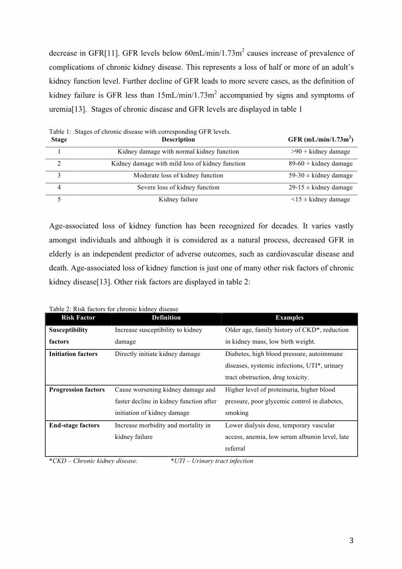
decrease in GFR[11]. GFR levels below 60mL/min/1.73m2 causes increase of prevalence of

complications of chronic kidney disease. This represents a loss of half or more of an adult’s

kidney function level. Further decline of GFR leads to more severe cases, as the definition of

kidney failure is GFR less than 15mL/min/1.73m2 accompanied by signs and symptoms of

uremia[13]. Stages of chronic disease and GFR levels are displayed in table 1

Table 1: Stages of chronic disease with corresponding GFR levels. Stage Description GFR (mL/min/1.73m2)

1 Kidney damage with normal kidney function >90 + kidney damage

2 Kidney damage with mild loss of kidney function 89-60 + kidney damage

3 Moderate loss of kidney function 59-30 ± kidney damage

4 Severe loss of kidney function 29-15 ± kidney damage

5 Kidney failure <15 ± kidney damage

Age-associated loss of kidney function has been recognized for decades. It varies vastly

amongst individuals and although it is considered as a natural process, decreased GFR in

elderly is an independent predictor of adverse outcomes, such as cardiovascular disease and

death. Age-associated loss of kidney function is just one of many other risk factors of chronic

kidney disease[13]. Other risk factors are displayed in table 2:

Table 2: Risk factors for chronic kidney disease

Risk Factor Definition Examples

Susceptibility

factors

Increase susceptibility to kidney

damage

Older age, family history of CKD*, reduction

in kidney mass, low birth weight.

Initiation factors Directly initiate kidney damage Diabetes, high blood pressure, autoimmune

diseases, systemic infections, UTI*, urinary

tract obstruction, drug toxicity.

Progression factors Cause worsening kidney damage and

faster decline in kidney function after

initiation of kidney damage

Higher level of proteinuria, higher blood

pressure, poor glycemic control in diabetes,

smoking

End-stage factors Increase morbidity and mortality in

kidney failure

Lower dialysis dose, temporary vascular

access, anemia, low serum albumin level, late

referral

*CKD – Chronic kidney disease. *UTI – Urinary tract infection

4

Due to the adverse outcomes of decline in renal function mentioned earlier, assessing GFR is

of great importance in clinical practice. GFR can either be estimated based on endogenous

markers, using validated algorithms, or accurately measured by exogenous probes. Clearance

techniques used to measure GFR could involve endogenous (creatinine, urea) or exogenous

(inulin, iohexol, iothalamate) filtration markers. GFR estimations are, most often, sufficient

in clinical practice but the accurately measured GFR is required in certain cases[14]. Renal

transplant recipients, potential kidney donors or research studies use a more accurate

assessment of renal function, thus requiring a formal measurement of GFR[10]. Infusion of

an exogenous agent is required to measure GFR due to the non-existence of an ideal

endogenous substance for GFR measurement.

Certain strict physiological characteristics are required for a substance in order for it to be

useful as a marker or a reference method for GFR. These include production and plasma

concentration of the marker being constant if GFR does not change, exclusive excretion by

kidneys and mainly via filtration through the glomerulus, non-secretion nor absorption by

renal tubules. The marker should also be easily measured in plasma and also urine and non-

toxic[14]. It does not matter if the renal function markers are endogenous or exogenous, but

for accurate assessment of GFR only exogenous markers are currently used.

1.1.4 eGFR Acquiring the “true” GFR by measurement of clearance of a marker can be cumbersome and

costly, thus making GFR estimations more attractive in clinical practice[15]. Estimated GFR

is often good enough for monitoring changes in renal function in an individual patient over

time. It also forms the basis for classification of chronic kidney disease.

Endogenous markers (Creatinine)

The most widely used endogenous method of reference is serum creatinine concentration.

Creatinine is a breakdown product of creatinephosphate in muscle tissue, produced at

relatively constant rate, depending on muscle mass. It is inexpensive and generally accessible

to measure. Serum creatinine and urinary creatinine clearance are methods of estimating GFR

with creatinine. Serum creatinine measurements are easy and fairly precise, making it an

attractive alternative in clinical practice[16]. Creatinine levels in the blood increase with

decreasing renal function and serum creatinine levels can be used to calculate GFR[17].

5

Urinary creatinine clearance is highly dependent on the accuracy of urine collection[16].

Urine is collected for 24 hours and creatinine levels measured in the urine determines the

clearance of creatinine, which is supposed to be correlated to GFR. Secretion of creatinine by

the renal tubules causes this method of measurement to overestimate GFR[18].

The result of using creatinine as a marker is estimation and not an accurate measure of GFR.

Several factors such as sex, age, race, muscle mass and dietary protein intake contributes to

the reduction of creatinine’s accuracy as an indicator of GFR[18]. Due to these influences,

several equations have been formulated to correct the inaccuracy. The formulas have been

developed using data from patients with chronic kidney disease[16].

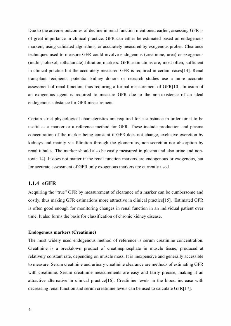
An approximate amount of over 40 different prediction equations are available for

determining GFR using creatinine as a marker but only three of them are commonly used.

Two of the equations (displayed in figure 1) are Cockcroft-Gault and “Modification of Diet

in Renal Disease”(MDRD) formulae[19, 20]. The third type is CKD-EPI, a set of new

equations developed in recent years.

New equations have been developed in recent years. These equations are have been

implemented into clinical practice as a general test for assessing GFR in adults. They have

been developed for use with standardized serum creatinine assays, as has implementation of

new equations developed for use with standardized cystatin c as “confirmatory tests” for

decreased eGFR have been proposed in clinical practice. The most accurate GFR estimating

equations in large diverse population in recent times are The Chronic Kidney Disease

Epidemiology Collaboration (CKD-EPI) equations. The 2009 CKD-EPI creatinine equation

was developed to improve on the 2006 MDRD Study equation due to its limitations. The

variables included in both equations are the same but they differ in form and coefficients[21].

A comparison of the equations used to estimate GFR prove that the CKD-EPI equations are

more accurate than the MDRD Study equation. The CKD-EPI is less biased in most

subgroups defined by demographic and clinical characteristics and level of GFR[22, 23],

meaning there is less of a systemic difference between eGFR and GFR.

6

Figure 1: Prediction equations based on plasma creatinine for estimating GFR CKD-EPI, Cockroft Gault and MDRD are prediction equations for determining GFR using creatinine as a marker

1.1.5 mGFR Exogenous markers

Exogenous markers are in certain cases required, due to the limited accuracy of the

endogenous markers. Planning cancer chemotherapy with nephrotoxic agents, staging chronic

kidney disease or preparations for renal replacement therapy are typical cases in which the

utilization of a more definite measurement of GFR is necessary[24]. If the nonrenal clearance

of a substance is negligible, the substance’s plasma clearance is directly correlated with renal

clearance of said substance. A single-injection clearance technique can then be used to

calculate GFR by monitoring the substance’s rate of disappearance from the plasma after the

injection[25]. A continuous intravenous infusion is also a possibility in combination with

urine collection and concentration measurements in both plasma and urine for calculation of

clearance[26].

The gold standard of mGFR is inulin clearance. Inulin possesses all the attributes required to

be a marker of GFR measurement and is known as the ideal marker for determining GFR yet

technical difficulties inherent in the measurement of inulin concentration in urine and in

plasma creates limitation in its utility in clinical practice. Alternatives to inulin as an

exogenous marker are radioactive agents such as 51Cr-EDTA, 99mTc-DTPA, and 125I or

7

131Iothalamte. However, there are problems with each of these agents and none of them are

regarded as adequate replacements for the standard inulin clearance. Another alternative that

has proved to be a satisfactory marker of GFR both in adults and children is Iohexol.

1.1.6 Iohexol

Figure 2: Iohexol molecular structure[27]

Iohexol Properties

Iohexol is a nonionic contrast medium[28]. It has a molecular weight of 821 Dalton and is

used intravenously for radiologic procedures. Iohexol is neither secreted, metabolized nor

reabsorbed by the kidney. It diffuses into the extracellular space and it binds less than 2% to

plasma proteins. Iohexol is eliminated exclusively via filtration in the kidneys. There are two

isomers of iohexol and they both, are handled similarly by the body. Radiolabeled iohexol is

a possibility of measurement but less attractive than measurements of serum concentrations

with HPLC-UV[24].

Single-injection Approach

Iohexol-determined GFR is based on a single injection of Omnipaque®, the brand name of

iohexol, and the analyses of blood samples from the patient. According to protocol utilized at

OUS-Rikshospitalet, Omnipaque®[29] is injected using a venflon or a threeway-split

butterflysyringe. Due to accuracy of the procedure, the whole volume has to be injected and

the exact injection volume recorded. For Omnipaque 300mgJ/ml, the recommended dosage is

2 mL for children below the age of two and 5 mL for all patients above the age of two. The

exact injection volume is achieved by weighing the syringe before and after the injection. The

patient’s weight and height are also required for algorithm after the sample analyses[29].

8

Plasma clearance and sample analyses

Duration of plasma disappearance and number of blood sample collections are important

decisions made when using iohexol as a marker[30]. The algorithm used for measurement

can calculate the patients GFR using either one time-specific blood sample or two time-

specific blood samples. They are respectively referred to as One-point or Two-point

measurements. Two-point measurements give more accurate calculations of GFR and are

highly recommended when children are involved[29]. Schwartz et al [24] discovered that

two sample measurement of iohexol disappearance was just as adequate as a four sample and

a nine sample measurement. When using two-point measurement, the first sample cannot be

taken earlier than 120min after injection and the last sample should not be obtained earlier

than 300min after injection. These are sampling times that describe the elimination of

iohexol. Timing of the second and last sample depends on the individuals renal function[24].

The recommended time periods for blood sampling in relation to individuals estimated GFR

according to the protocol at OUS-Rikshospitalet are displayed in the table 3.

Table 3: Protocol for sampling times at OUS-Rikshospitalet

GFR >40 GFR 10-40 GFR >10

One-point

measurement

3 hours after injection 8 hours after injection 24 hours after injection

Two-point

measurement

2 and 5 hours

after injection

2 and 8 hours

after injection

2 and 24 hours

after injection

The time of blood sampling does not have to be exact. A leeway of 15 minutes is accepted,

given that the exact time of injection and blood sampling is recorded. The blood is collected

and sent for centrifugation. A minimum of 0.6mL blood (0.3 mL serum) is required. The

samples are then analyzed using HPLC-UV (liquid chromatography)[29].

Clinical algorithm

The iohexol concentrations achieved from the HPLC analyses are used in an algorithm to

calculate a patient’s true GFR. The GFR is based on calculation from the dose of the iohexol

divided by area under the plasma disappearance curve (AUC0-inf), displayed in equation (1),

fitted by a double exponential equation.

(1) 𝐶𝑙𝑒𝑎𝑟𝑎𝑛𝑐𝑒 = !"#$!"#!!!"#

9

The total AUC0-inf of iohexol can be divided into two mono exponential decay curves by the

residual method. The first curve describes distribution of iohexol and second curve describes

elimination. To approximately determine both curves, at least 4 blood samples between 5

minutes and 5 hours after injection are needed. These time periods describe both distribution

and elimination of iohexol relatively accurate. Concentrations achieved from the two blood

samples are used to determine the AUC by determining the elimination curve. The

distribution curve then has to be estimated to be able to determine the whole AUC[24]. Using

this technique, the GFR for patients with expanded body spaces are overestimated. This

includes patients with oedema or ascites and this technique may be inadequate. Most patients

within this groups are highly dependent on accurate GFR measurement due to accuracy in

chemotherapeutic regimes[31].

The clinical algorithm combines the patient’s anthropometry (height, weight, sex) with

amount and concentration of iohexol given and time of blood sampling to determine the

elimination phase. The distribution phase is then estimated based on previous population

values and initial estimates of GFR. The result is the patient’s GFR in ml/min/1.73m2. That

value is then adjusted based on the patient’s body surface area. The result is divided by

1,73m2, resulting in the patients GFR[24].

1.2 Population modeling 1.2.1 Population Pharmacokinetics Population pharmacokinetics is the study of the sources and correlates of variety in drug

concentrations among individuals who are the target patient population receiving clinically

relevant doses of a drug of interest[32]. The aim is to identify and quantify sources of the

variability. Associations between patient characteristics and differences in pharmacokinetics

can then be used to customize individual prediction of pharmacokinetic parameters[1]. One

of the major differences between population pharmacokinetics and the traditional form of

non-compartmental analyses of pharmacokinetic study is the samples needed for analyses.

Traditionally, healthy volunteers were required and multiple samples were taken at fixed

intervals. In contrast, patients involved in population pharmacokinetic studies are patients

taking different doses of the drug investigated and blood samples are taking at different

times. The use of population pharmacokinetics has vastly increased in the field of drug

10

development, especially in situations with suspicion of highly variable pharmacokinetics of a

drug between subgroups of the population[1].

1.2.2 Population Pharmacokinetics models Pharmacokinetic modeling is a mathematical method for predicting how the body will handle

a drug[1]. It is a concept that involves an estimation of an unknown population distribution

based on data from a collection of non-linear models[33]. The primary goal is finding

population pharmacokinetic parameters and sources of variability in a population. Observed

concentrations relations to administered doses by identifying predictive covariates in a target

population are another goal when using population models. The need for many observations

per subject, also referred to as “rich” data, is not as highly required when using a population

model as it is in analysis of single-subject data. Structured sampling time schedules are not a

requirement either. Few observations per subject, also referred to as “sparse” data, or a

combination of “sparse” and “rich” data can be used when working with a population

pharmacokinetics model[34].

Three important components of population modeling are structural, stochastic and covariate

models. The structural models describe the time course of a measured response. It is normally

represented as algebraic or differential equations. The stochastic model describes variability

or random effects in the observed data. Other factors may influence individual time course of

a response. These factors can be the patient’s demographics or a disease and they are

described with covariate models[34, 35].

Estimating a typical value, such as drug clearance or oral bioavailability, is normally the

point of interest in population pharmacokinetics. Each patient lends information to the

population model but then borrows information back from the population model to obtain an

estimate of their own pharmacokinetic parameters. This means the individuality of the

information supplied by each patient to the population is used to estimate the most likely

value of the parameter for each patient. This typical parameter value is usually the most

frequent occurring value (the mode) and approaches the population mean value as the number

of patients increase. Pharmacometrics can be used to improve our understanding of

mechanisms, inform the initial selection of doses to test or personalize dosage for

subpopulations of patients and evaluate the appropriateness of the study designs[35].

11

1.2.3 Pmetrics Pharmacometrics is the incorporation of pharmacokinetics and pharmacodynamics models

and simultations[36]. Pmetrics is a pharmacometric library package for R, a statistical and

programming software. The Pmetrics package is for simulation and parameter estimation in

linear and non-linear pharmacokinetic/pharmacodynamics systems.

Installation of three components is required when taking use of the Pmetrics package. The R

software, Pmetrics package for R and gfortran, a fortran complier. There are three main

software programs that Pmetrics control: IT2B, NPAG and a semi-parametric Monte Carlo

simulation software program. The software program used in this study is NPAG[36]

NPAG: Non-parametric adaptive grid

This software creates non-parametric population models. The models consist of discrete

support points, each with a set of estimates, and an associated probability of that set, for all

parameters in the model. Each subject in the study population represents, at most, one support

point[36].

The values of the model parameters in the population, such as clearance, are random effects.

NPAG has no need to make any assumptions about the underlying distribution of random

effects. The fixed effect is the error model. This consists of a polynomial that describes assay

variance. It also consists of a multiplier of assay variance or an addend to assay variance,

respectively referred to as gamma and lambda. They are each estimated as a single value in

the population[36]

Akaike Information Criterion( AIC)

AIC is an estimate of a measure of fit of a model. The model and the model’s parameters

define it, which then gives the minimum of AIC. AIC estimates describe how structured a

model is compared to other models[37].

12

1.3 Aim of the study The aim of the study is to create a population pharmacokinetic model for iohexol that can be

used to determine glomerular filtration rate.

The specific goals for the model are:

- Defining how few sampling times that accurately will determine GFR

- Defining optimal sampling times for measuring GFR in renal transplant recipients.

13

2 Material and methods 2.1 The Patients 13 renal transplant recipients from OUS-Rikshospitalet were included in this study.

An in-depth investigation, including the measured GFR is performed in all renal transplant

recipients 8 weeks and 1 year after transplantation. The current method for measuring GFR in

these patients is a two-point iohexol method where blood sampling is performed at two and

five hours after iohexol injection if eGFR is >40mL/min, 2 and 8 hours if eGFR is between

40 and 15 mL/min and 2 and 24 hours if eGFR is <15mL/min. For this study, patients

meeting at the Laboratory for renal physiology for a measured GFR investigation were asked

to donate up to ten additional blood samples following iohexol administration. In patients

with an eGFR >40ml/min sampling for at least 5 hours were requested and for those with

eGFR > an additional 3 samples were warranted between 5 and 24 hours.

2.2 Iohexol analyses A high performance liquid chromatography (HPLC) system is used to determine iohexol. An

isocratic mobile phase with a pH value of 2.5 is prepared using:

- 50mL acetonitrile (C2H3N)

- 950mL deionized water

- 1mL ortho-phosphoric acid 88%

The specimen is mixed with 800uL of perchloric acid 5% and vortex mixed for 30 seconds. It

is then centrifuged at 10900 rpm for 6 minutes. The supernatant is placed into an autosampler

vial and a 50uL of the specimen volume is injected onto the column[38].

2.2.1 Calibration Calibration of the method is performed using the same iohexol used for clearance estimation.

The calibrators consist of omnipaque solution and pure serum/plasma. An omnipaque

solution with a concentration of 1.8mg/mL is made and mixed with the serum/plasma[39].

The calibrator concentrations are presented in table 4.

14

Table 4: Calibrator concentrations[39] Calibrator Concentration Total volume Omnipaque

solution

Serum/plasma

volume

Calibrator_10 10ug/mL 10mL 56uL 9,944mL

Calibrator_50 50ug/mL 10mL 278uL 9.722mL

Calibrator_100 100ug/mL 10mL 556uL 9.444mL

The calibrators are mixed and distributed to Nunc-cylinders. 500uL are collected to each

cylinder and frozen down at -20 degrees[39].

2.2.2 Analyses The calibrator chromatogram determines iohexol retention time. Iohexol consists of 2

chromatogram peaks and the second peak is used to determine GFR. 3 calibrators are

analyzed for each series of serum/plasma analyzed. The results of the iohexol analyses are

documented (mg iodine/mL) in an excel sheet, together with patient’s demographics, dosage

and blood sampling times[39].

2.3 Iohexol population model development The software used for pharmacokinetics analyses in this study is Pmetrics version 1.3.1. The

software requires two forms of data input for the analyses, an input file and a model file.

Input file

The input file is an excel spreadsheet format with data needed to describe the population. The

order, capitalization and names of the header of the first 12 columns are fixed. The first 12

columns have to be “Id, evid, time, dur, dose, addl, ii, input, out, outeq, c0, c1, c2 and c3”.

Column descriptions are displayed in table 5

Table 5: Description of fixed columns in the input file. Columns Description

ID A numeric character that identifies each individual

Evid The event ID field. 0= observation, 1= Input(e.g dose) 4= reset

Time Elapsed time in decimal hours since the first event.

Dur Duration of an infusion, in hours. (0 for oral doses)

Dose The dose amount.

15

Addl Specifies the amount of additional doses.

ii Specifies the interdose interval

input This defines which input (i.e drug) the dose corresponds to.

Out This is the observation or output value (e.g drug concentration)

Outeq The output equation that corresponds to the OUT value

C0,c1,c2, c3 These are coefficients for the assay error polynomial for that observation.

The next columns are the patient’s demographics and covariates used in the model file. There

are no requirements to how the names and order of these columns have to be. Iohexol dosage

is documented in the first row for each patient under the “dose” column. The value under the

“time” column is “0” and the value under the “evid” and “input” columns is “1” indicating

that the row represents dose input of drug nr.1 (Pmetrics can handle up to seven drugs

simultaneously). The next rows after, for each patient, consist of the sampling times and the

corresponding plasma iohexol concentration. The value under “evid” is “0” for observation

and the value under “outeq” is “1” (for drug nr.1), indicating that the row represents an

observation and not a dose input. The concentrations are documented under the “out”

column. Covariate values are updated if relevant in each new row[36].

There are certain requirements to some of the columns in the input file. The time periods are

documented in the input file as relative times (hours) after injection of iohexol. The doses in

the input file are documented in milligrams. The concentration of omnipaque used for GFR

measurement is 300mg iodine /mL. This is equivalent to 647mg iohexol/mL. The iohexol

concentrations achieved from the HPLC analyses are converted (iodine:iohexol ratio =2.16)

and documented under the “out” column in mg/L iohexol. The documentation of the

patient’s sex in the input file has to be numeric for recognition in the R software. The number

“1” is for males and “0” for females. The values in the weight and height columns are

documented in kilograms and meters.

The values can be either documented in the excel file and imported to the R software for

modification or they can be both documented and modified in excel before import to the R

software[36].

16

Model file

The model file is a text file with up to 11 blocks, each marked by “#” followed by header

tags. The model file is the data input containing the primary variables (with boundaries

defined) and covariate equations for the model. The blocks used in this study are #PRImary

variables, #COVariates, #SECondary variables, #DIFferential equations, #OUTput and

#ERRor. The primary variables are the parameters that are estimated by Pmetrics. The

secondary variables are defined by equations that are combinations of primary variables and

covariates. In the model file, clearance (CL), volume of distribution (V), peripheral volume

of distribution (Vp) and intercompartmental clearance (Q) were set up as primary variables.

Different secondary variables and covariates were applied in the model file[36].

Different types of compartment models had to be tested to find the best structural model for

the distribution and elimination of iohexol. Two and three compartment models were tested

and compared. Two-compartment models were coded algebraically while three-compartment

models were coded with differential equations, as algebraic equations cannot handle more

than two compartments. Extracts of the model files are displayed in figure (3) and (4).

Two-compartment model: #PRI CL0 V0 Vp0 Q0 #SEC WTc= WT/72 CL = CL0*WTc**0.75 V = V0*WTc Vp =Vp0 Q = Q0 Ke = CL/V KCP = Q/V KPC = Q/Vp Figure 3: Model file extract

Three-compartment model #PRI V1S, 1,50 K10, 1, 50 K12, 1,30 K21, 1, 45 K23, 1, 60 #SEC WTc=WT/72 V1= V1S*WTc V2= V2S V3= V3S #DIF XP(1)= RATEIV(1) + K21*X(2)-K12*X(1)- K10*X(1) XP(2)= K12*X(1)- K21*X(2)+ K32*X(3)- K23*X(2) XP(3)=K23*X(2)- K32*X(3) Figure 4: Model file extract

17

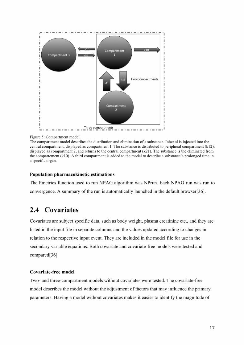
Figure 5: Compartment model. The compartment model describes the distribution and elimination of a substance. Iohexol is injected into the central compartment, displayed as compartment 1. The substance is distributed to peripheral compartment (k12), displayed as compartment 2, and returns to the central compartment (k21). The substance is the eliminated from the compartement (k10). A third compartment is added to the model to describe a substance’s prolonged time in a specific organ.

Population pharmacokinetic estimations

The Pmetrics function used to run NPAG algorithm was NPrun. Each NPAG run was run to

convergence. A summary of the run is automatically launched in the default browser[36].

2.4 Covariates Covariates are subject specific data, such as body weight, plasma creatinine etc., and they are

listed in the input file in separate columns and the values updated according to changes in

relation to the respective input event. They are included in the model file for use in the

secondary variable equations. Both covariate and covariate-free models were tested and

compared[36].

Covariate-free model

Two- and three-compartment models without covariates were tested. The covariate-free

model describes the model without the adjustment of factors that may influence the primary

parameters. Having a model without covariates makes it easier to identify the magnitude of

18

influence a specific factor has on perfecting the model’s ability to predict the observed

values.

Covariates

Different covariates were tested in this study. The covariates tested were based on

pharmacokinetic parameters with a theoretical potential to influence the pharmacokinetics of

iohexol. Allometric scales were performed. Clearance parameters were multiplied with the

centralized body size measures (Weight, height and BMI) to the power 0.75 and volumes to

power of 1. Median covariate values for the population were used for centralization.

The covariates “age” and “plasma creatinine” were also tested. They were first multiplied

with the primary parameters and later combined with the body size measures. The idea was to

investigate if these covariates influenced the model on their own or influenced the model by

enhancing the influence of body size measures.

All covariates models tested in this study were evaluated by comparing r-squared values, bias

and imprecision. Changes in AIC was minimal and therefore eliminated as a unit of

comparison. Further investigation was inhibited for covariate models that showed no

improvement (covariate-free models as reference).

2.5 Calculating GFR “makeNCA “ is a Pmetrics function used to calculate AUC0-inf for each individual in the input

file, using the trapezoidal approximation. AUC0-inf was calculated with the observed values

for each individual. Iohexol dosages for each patient were then divided by the patient’s

corresponding AUC value, resulting in their clearance (L/h). Based on our assumption that

clearance of iohexol is directly correlated to renal clearance, the patients GFR value

(mL/min) is equal to the iohexol clearance. The value is simply converted from L/h to

mL/min. equations are displayed as (2) and (3) The GFR values calculated from the observed

values were used as reference.

(2): Clearance(L/h) = Dose/AUC0-inf (3): GFR(ml/min) = CL* (1000/60)

19

2.6 Clinical algorithm An excel file, incorporated with the clinical algorithm was used to calculate GFR.

Information required for the clinical algorithm was:

- Sex

- Child or adult

- Iohexol concentrations at 2 and 5 hours after administration (mg iodine/ L)

- The specific time of iohexol administration (hours:minutes)

- The time periods for 2 and 5 hours concentrations (hours:minutes)

- Weight and height

- Volume of Ominipaque injected (mL)

- Omnipaque concentration (mg iodine/mL)

After plotting the values into the file, GFR was calculated by the algorithm, resulting in a

value with the unit mL/min/1.73m2. The value was adjusted with patient’s body surface area

value, resulting in the patient’s GFR.

2.7 Two-point and three-point measurements The MMopt function in Pmetrics was used to find the optimal sampling times for the model.

A new input file was created with two test persons and standardized sampling times outlined.

The covariates were different for the two test persons in order to get the MMopt function to

estimate sampling times over a relevant range of potential patients. The demographics of the

two representative test patients in the input file is displayed in table 6.

Table (6): Representative test patient demographics for estimation optimal sampling times using the MMopt() function in Pmetrics

Patient Age Sex Weight Height BMI

1 62 M 76.9 1.8 24

2 21 F 95.5 1.7 33

The MMopt() function was run to determine both two- and three optimal sampling times

within the first 5 hours after iohexol administration. The sampling interval was based on

intervals in the input file.

20

The sampling time closest to those determined from the MMopt function was used for

patients which did not have a sample drawn at the exact time periods according to the MMopt

results. The same was done for the three-point measurements test. The input files were

imported in the R software together with the model file from the final model and simulations

were run. New patient input files were created only including the measurements according to

the MMopt results, i.e. 2 or 3 samples.

2.8 Comparing GFR-values GFR values from the two- and three-point measurements were calculated with the same

method as the reference. The GFR values calculated from the two- and three measurements

were compared to the GFR values calculated from the clinical algorithm, using the observed

values as reference.

A residual plot was used to display the comparison. GFR calculated from the clinical

algorithm and from the two- and three-point measurements were subtracted from the

reference and the difference was displayed in the residual plot.

21

3 Results 3.1 The Patients The demographics of the patients included in the study are displayed in table 7

Table 7: Patient demographics Patient Sex Post tx

[weeks]

Age

[years]

Height

[cm]

Weight

[kg]

BMI

1 M 8 49 187 101 29.0

2 M 8 62 179 76.9 24.0

3 M 8 57 180 79.3 24.5

4 F 8 54 161 63.8 24.6

5 M 8 60 178 84.0 26.5

6 M 8 46 183 113 33.6

7 M 8 63 184 82.2 24.3

8 F 8 56 178 69.3 21.9

9 M 8 21 170 95.5 33.0

10 M 8 25 177 66.9 21.4

11 M 8 60 187 82.8 23.7

12 M 8 55 184 82.6 24.4

13 M 8 37 181 90 27.5

Mean 49.6 179.2 83.6 26.0

SD 13.8 7.13 13.82 3.82

*M = male *F=female *tx=transplantation *BMI=body mass index *SD= standard deviation

22

3.2 Structural model The two-compartment model without covariates converged after 264 cycles. The three-

compartment model without covariates converged after 1011 cycles.

Figure(6): Observation-prediction plot The figure displays the observation-prediction plot for the two-compartment model. The plot describes the correlation between the observed and the predicted values, for both population and individual prediction

Figure (7): observation-prediction plot The figure displays the observation-prediction plot for the three-compartment model. The plot describes the correlation between the observed and the predicted values, for both population and individual prediction.

0 100 200 300 400

010

020

030

040

0

Population Predicted

Obs

erve

d

●

●

●

●

●

●

●

●

●

●

●●

●

●

●

●

●

●

●

●

●

●

●

●

●

●

●

●

●●

●

●

●

●

●

●

●

●

●

●

●

●

●

●●

●

●

●

●

●

●●

●

●

●

●

●●

●

●

●

●

●

●

●

●●

●

●

●

●

●

●

●

●

●

●

●

●

●

●●

●

●●

●

●

●

●

●

●

●

●

●

●

●

●

●

●

●

●●

●

●

●●

●

●

●

●

●

●

●

●

●

●

●●

●●

●

R−squared = 0.922Inter = 7.99 (95%CI −0.645 to 16.6)Slope = 0.906 (95%CI 0.858 to 0.953)Bias = 0.921Imprecision = 10

0 100 200 300 400

010

020

030

040

0

Individual Posterior Predicted

Obs

erve

d

●

●

●

●

●

●

●

●

●

●

●●

●

●

●

●

●

●

●

●

●

●

●

●

●

●

●

●

●●

●

●

●

●

●

●

●

●

●

●

●

●

●

●

●●

●

●

●

●

●●

●

●

●

●

●●

●

●

●

●

●

●

●

●●

●

●

●

●

●

●

●

●

●

●

●

●

●

●●

●

●

●

●

●

●

●

●

●

●

●

●

●

●

●

●

●

●

●●

●

●

●●

●

●

●

●

●

●

●

●

●

●

●●

●●

●

R−squared = 0.995Inter = 0.994 (95%CI −1.25 to 3.24)Slope = 0.999 (95%CI 0.986 to 1.01)Bias = −0.124Imprecision = 0.684

0 100 200 300 400

010

020

030

040

0

Population Predicted

Obs

erve

d

●

●

●

●

●

●

●

●

●

●

●●

●

●

●

●

●

●

●

●

●

●

●

●

●

●●

●

●●

●

●

●

●

●

●

●

●

●●

●

●

●

●●

●

●●

●

●

●●

●

●

●

●

●●

●

●

●

●

●●

●

●●

●

●

●

●

●

●

●

●

●

●

●

●

●

●●

●

●●

●

●

●

●

●

●

●

●

●

●

●

●

●

●●

●●

●

●

●●

●

●

●

●●

●

●

●

●●

●●

●●

●

R−squared = 0.921Inter = −7.01 (95%CI −16.4 to 2.38)Slope = 0.834 (95%CI 0.789 to 0.878)Bias = 5.11Imprecision = 12.1

0 100 200 300 400

010

020

030

040

0

Individual Posterior Predicted

Obs

erve

d

●

●

●

●

●

●

●

●

●

●

●●

●

●

●

●

●

●

●

●

●

●

●

●

●

●

●

●

●●

●

●

●

●

●

●

●

●

●

●

●

●

●

●●

●

●

●

●

●

●●

●

●

●

●

●●

●

●

●

●

●

●

●

●●

●

●

●

●

●

●

●

●

●

●

●

●

●

●●

●

●●

●

●

●

●

●

●

●

●

●

●

●

●

●

●

●

●●

●

●

●●

●

●

●

●

●

●

●

●

●●

●●

●●

●

R−squared = 0.988Inter = −2.98 (95%CI −6.45 to 0.502)Slope = 0.998 (95%CI 0.978 to 1.02)Bias = 0.478Imprecision = 1.5

23

The two-compartment model showed lower bias and imprecision values as seen in table (7)

Table (7): Values from run summaries

Two-compartment Three compartment

Bias Imprecision Bias Imprecision

Population 0.921 10 5.11 12.1

Individual 0.124 0.684 0.988 1.5 The table displays bias and imprecision values for both two-compartment and three compartment models. Lower bias and imprecision values describe a more structural model.

3.3 Covariate model 3.3.1 Two compartment model The three-compartment model showed no improvement with the allometric scaling. The

implementation of covariates was then carried on with two-compartment models, which

proved to have been positively influenced by the allometric scaling.

Table 8: Run summary from allometric scaling of the three-compartment model

K12/WTc^^0.25 K21/WTc^0.25

R-squared Bias Imprecision R-squared Bias Imprecision

Population 0.90 1.06 11.2 0.924 5.45 13.5

Individual 0.987 0.411 1.71 0.987 0.145 1.71

24

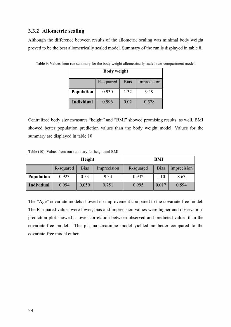
3.3.2 Allometric scaling Although the difference between results of the allometric scaling was minimal body weight

proved to be the best allometrically scaled model. Summary of the run is displayed in table 8.

Table 9: Values from run summary for the body weight allometrically scaled two-compartment model.

Body weight

R-squared Bias Imprecision

Population 0.930 1.32 9.19

Individual 0.996 0.02 0.578

Centralized body size measures “height” and “BMI” showed promising results, as well. BMI

showed better population prediction values than the body weight model. Values for the

summary are displayed in table 10

Table (10): Values from run summary for height and BMI

Height BMI

R-squared Bias Imprecision R-squared Bias Imprecision

Population 0.923 0.53 9.34 0.932 1.10 8.63

Individual 0.994 0.059 0.751 0.995 0.017 0.594

The “Age” covariate models showed no improvement compared to the covariate-free model.

The R-squared values were lower, bias and imprecision values were higher and observation-

prediction plot showed a lower correlation between observed and predicted values than the

covariate-free model. The plasma creatinine model yielded no better compared to the

covariate-free model either.

25

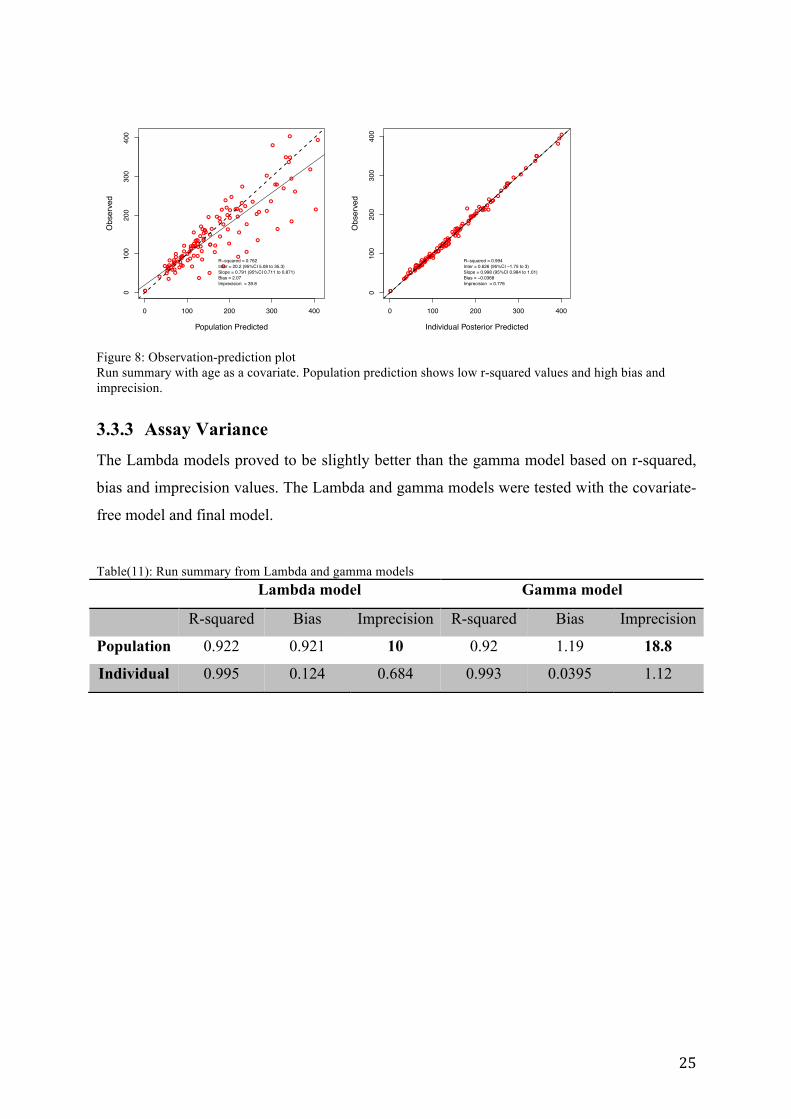
Figure 8: Observation-prediction plot Run summary with age as a covariate. Population prediction shows low r-squared values and high bias and imprecision.

3.3.3 Assay Variance The Lambda models proved to be slightly better than the gamma model based on r-squared,

bias and imprecision values. The Lambda and gamma models were tested with the covariate-

free model and final model. Table(11): Run summary from Lambda and gamma models

Lambda model Gamma model

R-squared Bias Imprecision R-squared Bias Imprecision

Population 0.922 0.921 10 0.92 1.19 18.8

Individual 0.995 0.124 0.684 0.993 0.0395 1.12

0 100 200 300 400

010

020

030

040

0

Population Predicted

Obs

erve

d

●

●

●

●

●

●

●

●

●

●

●●

●

●

●

●

●

●

●

●

●

●

●

●

●

●

●

●

●●

●

●

●

●

●

●

●

●

●

●

●

●

●

●●

●

●

●

●

●

●●

●

●

●

●

●●

●

●

●

●

●

●

●

●●

●

●

●

●

●

●

●

●

●

●

●

●

●

●●

●

●●

●

●

●

●

●

●

●

●

●

●

●

●

●

●

●

●●

●

●

●●

●

●

●

●

●

●

●

●

●

●

●●

●●

●

R−squared = 0.762Inter = 20.2 (95%CI 5.08 to 35.3)Slope = 0.791 (95%CI 0.711 to 0.871)Bias = 2.07Imprecision = 39.8

0 100 200 300 400

010

020

030

040

0

Individual Posterior Predicted

Obs

erve

d

●

●

●

●

●

●

●

●

●

●

●●

●

●

●

●

●

●

●

●

●

●

●

●

●

●

●

●

●●

●

●

●

●

●

●

●

●

●

●

●

●

●

●

●●

●

●

●

●

●●

●

●

●

●

●●

●

●

●

●

●

●

●

●●

●

●

●

●

●

●

●

●

●

●

●

●

●

●●

●

●

●

●

●

●

●

●

●

●

●

●

●

●

●

●

●

●

●●

●

●

●●

●

●

●

●

●

●

●

●

●

●

●●

●●

●

R−squared = 0.994Inter = 0.626 (95%CI −1.75 to 3)Slope = 0.998 (95%CI 0.984 to 1.01)Bias = −0.0368Imprecision = 0.776

26

3.4 The final model The final model was a two-compartment model that converged after 322 cycles with an AIC

value of 830 and 13 support points. Clearance and intercompartmental clearance were

multiplied with centralized body weight to the power of 0.75 while peripheral volume was

multiplied with centralized body weight to the power of 1. The observation-prediction plot is

displayed in figure 9.

Figure(9): Observation-prediction plot of the final model

Both input file and model file for the final model can be found in the appendix. The

secondary variables in the final model were: - CL=CL0*WTc**0.75

- V=V0

- Vp=Vp0*WTc

- Q=Q0*WTc**0.75

Predicted plasma concentration versus time plots for all 13 patients included, based on the

final model, was designed using the R software. Based on both R-squared values from the

observation-prediction plot and visual evaluation of the AUC-plots, this model was then used

to find the optimal sampling times for Omnipaque. The plots are displayed in figure (10).

0 100 200 300 400

010

020

030

040

0

Population Predicted

Obs

erve

d

●

●

●

●

●

●

●

●

●

●

●●

●

●

●

●

●

●

●

●

●

●

●

●

●

●

●

●

●●

●

●

●

●

●

●

●

●

●

●

●

●

●

●●

●

●

●

●

●

●●

●

●

●

●

●●

●

●

●

●

●

●

●

●●

●

●

●

●

●

●

●

●

●

●

●

●

●

●●

●

●

●

●

●

●

●

●

●

●

●

●

●

●

●

●

●

●

●●

●

●

●●

●

●

●

●

●

●

●

●

●

●

●●

●●

●

R−squared = 0.93Inter = 4.53 (95%CI −3.74 to 12.8)Slope = 0.911 (95%CI 0.866 to 0.956)Bias = 1.32Imprecision = 9.19

0 100 200 300 400

010

020

030

040

0

Individual Posterior Predicted

Obs

erve

d

●

●

●

●

●

●

●

●

●

●

●●

●

●

●

●

●

●

●

●

●

●

●

●

●

●

●

●

●●

●

●

●

●

●

●

●

●

●

●

●

●

●

●

●●

●

●

●

●

●●

●

●

●

●

●●

●

●

●

●

●

●

●

●●

●

●

●

●

●

●

●

●

●

●

●

●

●

●●

●

●

●

●

●

●

●

●

●

●

●

●

●

●

●

●

●

●

●●

●

●

●●

●

●

●

●

●

●

●

●

●

●

●●

●●

●

R−squared = 0.996Inter = −0.0813 (95%CI −2.17 to 2.01)Slope = 1 (95%CI 0.99 to 1.01)Bias = −0.0201Imprecision = 0.578

27

Figure (10): Plasma concentration vs time plot. The figure display the AUC plots created with prediction values from the final model. A robust model creates AUC plots with correlation to the observed values.

28

3.5 Two-point measurement vs Clinical algorithm Two-point and three-point measurements were tested in this study. The optimal sampling

times achieved from the MMopt function are displayed in table (12).

Table (12): Optimal sampling times based on…

Two-point measurement

Samples Time (hours)

Sample 1 0.5

Sample2 5

Three-point measurements

Samples Time (hours)

Sample1 0.5

Sample 2 1.5

Sample 3 5 The MMopt function in Pmetrics recommends optimal sampling times. These sampling times are the most descriptive and an accurate AUC plot can be created using concentration at these times.

Using the sampling times provided, AUC for each patient was predicted based on two and

three samples. The AUC values are displayed in table (13).

Table (13): AUC values

ID 2-pointmeasurement

3-pointmeasurement

Trapezoidalmethod

37 910.7 1173.0 945.838 784.3 784.3 798.642 880.6 876.2 853.144 1455.9 1160.0 1158.566 848.2 884.1 868.170 1983.7 971.2 741.274 1141.8 719.2 687.976 651.0 588.0 607.081 619.0 556.6 561.784 954.5 902.5 972.393 919.7 1896.9 901.694 1212.2 1786.2 982.897 887.2 875.4 893.7

AUC-values calculated for both two-point and three-point measurements using predicted concentration values. The reference was calculated with trapezoidal method using observed concentration values

29

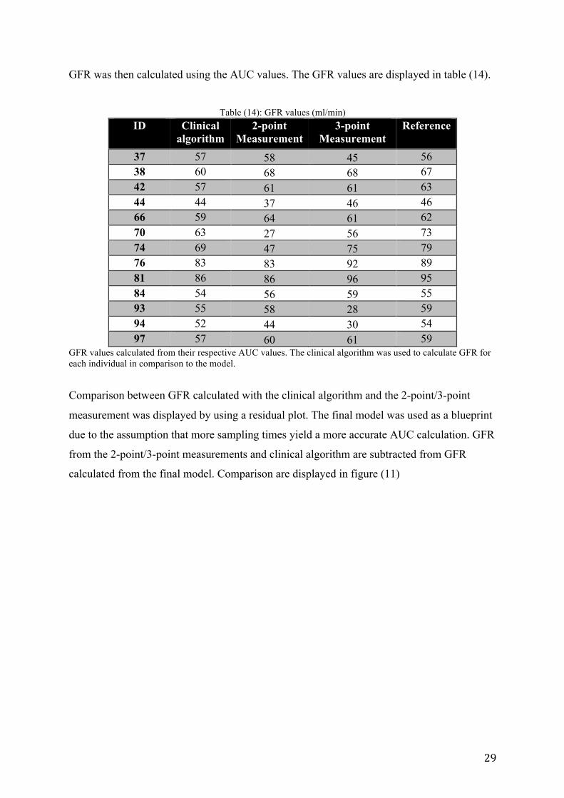
GFR was then calculated using the AUC values. The GFR values are displayed in table (14).

Table (14): GFR values (ml/min)

ID Clinical algorithm

2-point Measurement

3-point Measurement

Reference

37 57 58 45 56 38 60 68 68 67 42 57 61 61 63 44 44 37 46 46 66 59 64 61 62 70 63 27 56 73 74 69 47 75 79 76 83 83 92 89 81 86 86 96 95 84 54 56 59 55 93 55 58 28 59 94 52 44 30 54 97 57 60 61 59

GFR values calculated from their respective AUC values. The clinical algorithm was used to calculate GFR for each individual in comparison to the model.

Comparison between GFR calculated with the clinical algorithm and the 2-point/3-point

measurement was displayed by using a residual plot. The final model was used as a blueprint

due to the assumption that more sampling times yield a more accurate AUC calculation. GFR

from the 2-point/3-point measurements and clinical algorithm are subtracted from GFR

calculated from the final model. Comparison are displayed in figure (11)

30

Figure 11 shows the absolute difference between the trapezoidal-AUC derived GFR and the clinical 2-point algorithm GFR and the 2-and 3-sample model derived GFR, respectively. Values above 0 represent overprediction while values below 0 represent underprediction. Each number on the x-axis represents a patient

-50.0

-45.0

-40.0

-35.0

-30.0

-25.0

-20.0

-15.0

-10.0

-5.0

0.0

5.0

10.0

0 1 2 3 4 5 6 7 8 9 10 11 12 13 14

Clinicalalgorithm

2-pointmeasurement

Three-pointmeasurement

31

4 Discussion In this study, a population pharmacokinetics model was developed to determine glomerular

filtration rate in renal transplant recipients by using iohexol as a marker. The current clinical

practice is to determine measured GFR by using an algorithm that is based on calculation of

the elimination constant in the distribution phase of iohexol plasma concentration versus time

curve. One blood concentration two hours after administration is combined with a second

measurement after 5 to 24 hours, depending on the estimated renal function of the patient, to

determine elimination constant. The distribution phase and volume of distribution on the

other only is estimated based on population means and the individual patient’s demographics.

Benz de Bretagne et al[40] designed a bayesian model with iohexol samples obtained during

the elimination phase. A one-compartment model was the best model that described the

data[40]. The final model that best described the population in this study was a two-

compartment model with primary parameters allometrically scaled by centralized body

weight. Based on this model, optimal sampling times for measuring GFR in renal transplant

recipients were determined to be 30 minutes and 5 hours after iohexol administration for two-

point measurement. For a three-point measurement, optimal sampling times were 30 minutes,

1.5 hours and 5 hours after iohexol administration.

4.1 The patients 13 renal transplant recipients were included in this study. All 13 renal transplant recipients

were in the early post transplant phase 8 weeks after transplantation, and 2 of the 13 had an

estimated GFR < 40 mL/min. This is in accordance with the general renal transplant recipient

in Norway. When having an estimated GFR less than 40 mL/min the protocol for mGFR

measurement using iohexol indicate that the last sample should be taken 8 hours after

administration, which is cumbersome in a policlinic setting. The present iohexol population

model indicate that also these patients will be able to get an accurate mGFR determination

just using samples up to 5 hours after administration.

32

4.2 Evaluating the model Between nine to twelve iohexol samples were obtained per individual in the period 5 minutes

to 5 hours after administration of iohexol. The total of the samples were able to describe both

the distribution and elimination phase of iohexol well in the population

Evaluation of the models was based on bias, imprecision and r-square of the observation-

prediction plots. Two- and three-compartment models were tested and compared. As

expected, the two-compartment model proved to be the better model based on the available

values. The two-compartment observation-prediction plot showed better correlation between

predicated and observed values for both population and individual predictions.

Implementation and investigation of the covariates was carried on with the two-compartment

model due to lack of improvement in evaluation values for the three-compartment model.

The primary parameters were multiplied with centralized body size measures to the power of

0.75 for clearance parameters and to the power of 1 for the volume parameters. Minimal

difference in r-squared was registered for the values with and without allometrical scaling.

The difference was noticed in the bias and imprecision values. Bias and imprecision values

were lower for the body size measure models with allometric scaling. The allometrically

scaled model showed higher r-squared values for both the population and individual

predictions than the model without covariates. The improved r-squared values compared to

the non-scaled model indicate that the allometric scaling of the primary parameters improved

the models ability to estimate both population and individual predicated concentrations.

Population prediction bias was lower for the model without covariates but bias for individual

prediction and imprecision was lower for the allometrically scaled model.

33

4.3 Covariates Allometrically scaled height and BMI models showed improved bias and imprecision values

compared to the model without covariates but allometrically scaled body weight showed a

higher improvement in the evaluation values. Clearance, intercompartmental clearance and

peripheral volume were allometrically scaled to centralized body weight in the final model.

Both “age” and “plasma creatinine” were investigated as potential covariates in the model.

The covariate models tested, were developed by multiplying the primary parameters with the

centralized covariates. Age did not show any relevant effect on the model while plasma

creatinine showed a distinctive difference on the population observation-prediction plot. R-

squared values as low as 0.5 were registered. As iohexol is fully dependent on renal

elimination it was expected that plasma creatinine whole have such an effect on the

population prediction in the iohexol model. The incorporation of plasma creatinine in the

model reduced however its ability to estimate individual predictions. This is probably due to

the fact that plasma creatinine is a worse marker of renal function than iohexol itself and

including this covariate will introduce a new variability in the model. Since the aim of the

development of the population model is to determine mGFR and it will never be an issue to

utilize it without actually having iohexol concentration measurements available the model

without covariates were chosen to be the most appropriate model for the present objective.

4.4 Validation Measuring the performance of the model’s predictive abilities can test the validity of a

population model. This is done by either testing the same dataset (internal validation) or

testing on a different dataset of new patients. (external validation).

Internal validation

Internal validation in this study was performed through model evaluation during the

development. Visual evaluation of the observation-prediction plot was the method used to

internally validate the dataset. Normal methods of internal validation are jack knife

validation, likelihood-based method and cross-validation analysis. None of these methods

were used in this study due to the limited number of subjects included in the study so far.

34

External validation

The model was not externally validated due to the lack of an evaluation population. The

number of patients included was not sufficient for both building the model and validating the

model. Generally, a group of new patients are used to validate the model but due to time

constraint and inclusion conditions, 13 patients were included and only used to build the

model.

4.5 Comparing GFR values The aim of the study was defining optimal sampling times for measuring GFR in renal

transplant recipients. Two- and three-point sampling were tested and compared with both

each other and the algorithm utilized in clinical practice. The algorithm utilized in clinical

practice is an algorithm based on the calculations that measure the elimination phase of

iohexol disappearance, meaning the distribution phase is only estimated. The model on the

other hand estimated the most plausible full-PK curve for each individual with the utilization

of two- or three-point measurements. This includes hence and individual estimation of both

the distribution and elimination phase of individuals, potentially giving a more complete

description of iohexol disappearance in each individual.

AUC0-inf was calculated with the trapezoidal method using the observed concentrations. This

was used as reference. GFR calculated from the clinical algorithm showed a relatively even

distribution of GFR values close to the reference values. Although the clinical algorithm

showed a more even distribution than the two- and three-point measurements, the two- and

three- point measurements achieved results closer to the reference values in the majority of

the patients in this particular data set. In some cases however, the values were underpredicted

massively. Although both two- and three-point measurements based on the final model show

promising results, the massive underprediction is likely the result of lack of patients included,

especially patients with an estimated GFR less than 40 ml/min and demographic variety.

Underprediction as high as a difference of 45 ml/min was registered, indicating that the

model does not fully describe the population. More individuals need to be included in the

model before this method can be fully validated with regard’s to use in clinical practice.

35

4.6 Future perspectives Based on the results of the two- and three-point measurements, it is clear that the model has

the potential for future use in clinical practice. The sampling times utilized in this study seem

to accurately determine GFR based on the reference calculated with the trapezoidal method.

Due to the inclusion of few patients in the model, certain patients were massively

underpredicted. This indicates that future work on building a better model will require the

inclusion of more patients. Similarly, more patients are required in order to enable both

external and internal validation of the model. This will ensure more insight into the strengths

and weaknesses of the model.

36

5 Conclusion Using Pmetrics, a population pharmacokinetics model was designed to determine GFR in

renal transplant recipients. This was done in order to define optimal sampling times for

determining GFR.

The final model that best described the population in this study was a two-compartment

model with primary parameters allometrically scaled with centralized body weight. Future

work on building a better model will require the inclusion of more patients, especially more

data in the later post administration phase in patients with low renal function. More insight

into the strengths and weaknesses of the model will require validation of the model, either

internally or externally.

Preparations for renal replacement therapy require a more definite measurement of GFR. A

good population pharmacokinetic model could prove to be an invaluable tool for accurately

determining GFR, particularly in cases concerning patients with severe loss in renal function.

37

6 Referances 1. Charles,B.,Populationpharmacokinetics:anoverview.AustPrescr,2014.37:p.

210-3.2. Ratain,M.J.andW.K.PlunkettJr,PrinciplesofPharmacokinetics.2003.3. Candela,L.andC.Yucha,Renalregulationofextracellularfluidvolumeand

osmolality.(ContinuingEducation).NephrologyNursingJournal,2004.31(4):p.397.

4. Haug,O.,MennesketsFysiologi.Vol.1.2010:GyldendalNorskForlag.5. Hayashi,M.,Physiologyandpathophysiologyofacid-basehomeostasisinthe

kidney.InternMed,1998.37(2):p.221-5.6. Williams,S.,K.Malatesta,andK.Norris,VitaminDandchronickidneydisease.

EthnDis,2009.19(4Suppl5):p.S5-8-11.7. Sparks,M.A.,etal.,ClassicalRenin-Angiotensinsysteminkidneyphysiology.Compr

Physiol,2014.4(3):p.1201-28.8. Donnelly,S.,Whyiserythropoietinmadeinthekidney?Thekidneyfunctionsasa

critmeter.AmJKidneyDis,2001.38(2):p.415-25.9. Rang,H.P.,Pharmacology.Vol.7.2012:ElsevierInc.10. Traynor,J.,etal.,Howtomeasurerenalfunctioninclinicalpractice.British

MedicalJournal,2006.333(7571):p.733-737.11. Weinstein,J.R.andS.Anderson,Theagingkidney:physiologicalchanges.Adv

ChronicKidneyDis,2010.17(4):p.302-7.12. Allander,S.V.,etal.,Regionalvariationinuseofexogenousandendogenous

glomerularfiltrationrate(GFR)markersinSweden.UpsalaJournalofMedicalSciences,2012.117(3):p.273-278.

13. Levey,A.S.,etal.,NationalKidneyFoundationpracticeguidelinesforchronickidneydisease:evaluation,classification,andstratification.AnnInternMed,2003.139(2):p.137-47.

14. Delanaye,P.,Howmeasuringglomerularfiltrationrate?Comparisonofreferencemethods.2012:INTECHOpenAccessPublisher.

15. Xie,D.,etal.,Acomparisonofchangeinmeasuredandestimatedglomerularfiltrationrateinpatientswithnondiabetickidneydisease.ClinJAmSocNephrol,2008.3(5):p.1332-8.

16. Nankivell,B.J.,etal.,Predictingglomerularfiltrationrateafterkidneytransplantation.Transplantation,1995.59(12):p.1683-9.

17. Understandingyourlabvalues.2016;Availablefrom:https://www.kidney.org/kidneydisease/understandinglabvalues.

18. Santos,J.andL.S.Martins,Estimatingglomerularfiltrationrateinkidneytransplantation:Stillsearchingforthebestmarker.WorldJNephrol,2015.4(3):p.345-53.

19. Bhavsar,N.A.,etal.,ComparisonofmeasuredGFR,serumcreatinine,cystatinC,andbeta-traceproteintopredictESRDinAfricanAmericanswithhypertensiveCKD.AmJKidneyDis,2011.58(6):p.886-93.

20. Michels,W.M.,etal.,PerformanceoftheCockcroft-Gault,MDRD,andNewCKD-EPIFormulasinRelationtoGFR,Age,andBodySize.ClinicalJournaloftheAmericanSocietyofNephrology:CJASN,2010.5(6):p.1003-1009.

21. Levey,A.S.,L.A.Inker,andJ.Coresh,GFRestimation:fromphysiologytopublichealth.AmJKidneyDis,2014.63(5):p.820-34.

38

22. Stevens,L.A.,etal.,ComparativeperformanceoftheCKDEpidemiologyCollaboration(CKD-EPI)andtheModificationofDietinRenalDisease(MDRD)StudyequationsforestimatingGFRlevelsabove60mL/min/1.73m2.AmJKidneyDis,2010.56(3):p.486-95.

23. Levey,A.S.,etal.,Anewequationtoestimateglomerularfiltrationrate.AnnInternMed,2009.150(9):p.604-12.

24. Schwartz,G.J.,etal.,Glomerularfiltrationrateviaplasmaiohexoldisappearance:pilotstudyforchronickidneydiseaseinchildren.KidneyInt,2006.69(11):p.2070-7.

25. Schwartz,G.J.andD.F.Work,MeasurementandestimationofGFRinchildrenandadolescents.ClinJAmSocNephrol,2009.4(11):p.1832-43.

26. vanRossum,L.K.,etal.,Optimalsamplingstrategiestoassessinulinclearanceinchildrenbytheinulinsingle-injectionmethod.ClinChem,2003.49(7):p.1170-9.

27. Pharmacopeialforum.31March2016];Availablefrom:http://www.drugfuture.com/pharmacopoeia/usp32/pub/data/v32270/usp32nf27s0_m41920.html.

28. Olsson,B.,etal.,HumanPharmacokineticsofIohexol:ANewNonionicContrastMedium.Investigativeradiology,1983.18(2):p.177-182.

29. Bergan,S.GFRmålt(Nyrefunksjon).2016[cited201624April];Availablefrom:http://anx.no/gfr-maalt/.

30. Schwartz,G.J.,etal.,Optimizingiohexolplasmadisappearancecurvestomeasuretheglomerularfiltrationrateinchildrenwithchronickidneydisease.KidneyInternational,2010.77(1):p.65-71.

31. Perkinson,A.S.,etal.,Theeffectofimprovedmodellingofplasmaclearanceinpaediatricpatientswithexpandedbodyspacesonestimationoftheglomerularfiltrationrate.PhysiolMeas,2010.31(2):p.183-92.

32. U.SFoodandDrugAdministration.GuidanceforIndustry:PopulationPharmcokinetics.1999;Availablefrom:http://www.fda.gov/downloads/Drugs/.../Guidances/UCM072137.pdf.

33. Tatarinova,T.,etal.,Twogeneralmethodsforpopulationpharmacokineticmodeling:non-parametricadaptivegridandnon-parametricBayesian.JPharmacokinetPharmacodyn,2013.40(2):p.189-99.

34. Mould,D.R.andR.N.Upton,Basicconceptsinpopulationmodeling,simulation,andmodel-baseddrugdevelopment-part2:introductiontopharmacokineticmodelingmethods.CPTPharmacometricsSystPharmacol,2013.2:p.e38.

35. Mould,D.R.andR.N.Upton,Basicconceptsinpopulationmodeling,simulation,andmodel-baseddrugdevelopment.CPTPharmacometricsSystPharmacol,2012.1:p.e6.

36. Neely,M.N.,etal.,AccuratedetectionofoutliersandsubpopulationswithPmetrics,anonparametricandparametricpharmacometricmodelingandsimulationpackageforR.TherDrugMonit,2012.34(4):p.467-76.

37. Akaike,H.,ANewLookattheStatisticalModelIdentification.IEEETRANSACTIONSONAUTOMATICCONTROL,1974.19(6).

38. James,T.J.,etal.,Validityofsimplifiedprotocolstoestimateglomerularfiltrationrateusingiohexolclearance.(0004-5632(Print)).

39. Lauritsen,M.E.andT.Skogseth,Metodebeskrivelse:Glomerulærfiltrasjonsrate(GFR),HPLC,FAR,RH.2015,Seksjonerforkliniskfarmakologi-Rikshospitalet:OsloUniversitetssykhus,.

39

40. Benz-deBretagne,I.,etal.,NewsamplingstrategyusingaBayesianapproachtoassessiohexolclearanceinkidneytransplantrecipients.(1536-3694(Electronic)).

40

7 Appendix 7.1 Requisition for measured GFR with iohexol clearance

Målt GFR ved joheksol-clearance

ETIKETT

Avd. for farmakologi, OUS-Rikshospitalet Pb. 4950 Nydalen, 0424 OsloTlf.: 23071014 (Laboratoriet)

Av

delin

gfo

r fa

rmako

log

i, O

US

-Rik

sh

osp

itale

t

Kontaktinformasjon: Laboratoriet telefon 23071014.For mer info om GFR målt ved joheksol, se www.anx.no/GFR som også har kalkulator for utregningene samt denne rekvisisjonsblanketten for nedlasting. Dette finnes også på OUS intranett og internett under Avdeling for farmakologi.

Målt GFR forutsetter at pasienten får en infusjon av joheksol (Omnipaque). Det kan tas 1 eller 2 blodprøver til analyse av joheksol, 2 prøver gir den sikreste beregningen av GFR. Det er sterkt anbefalt å bruke 2 prøver ("2-pkt") konsekvent til barn; dette brukes ved Barneklinikken OUS. Dersom analysen haster, må laboratoriet kontaktes på forhånd.

Ved injeksjon av Omnipaque, anbefales å bruke venflon eller butterflykanyle med treveiskran. Pass på at hele volumetOmnipaque injiseres. Skyll deretter venflonen med 10 ml fysiologisk saltvann via treveiskranen.Blodprøvene tas i prøveglass uten tilsetning (rød kork) som sentrifugeres. Minimum 0,6 ml blod (0,3 ml serum).Enten man bruker 1-pkt eller 2-pkt må følgende informasjon angis for at GFR skal kunne regnes ut og bli rapportert:

Kroppsvekt: kg Høyde: cm

Det anbefales inj. volum Omnipaque 2 ml til barn under 2 år, ellers 5ml. Men NB: skriv alltid hva som faktisk blir gitt.Injisert Omnipaque 300 mg J/ml angis presist ved å veie opptrukket sprøyte før og etter injeksjon:

Vekt av sprøyte før inj. (med Omnipaque): gram -og etter injeksjon: gram

Injisert volum avlest fra sprøyte: ml

Tidspkt for inj. av Omnipaque 300mg J/ml, dato: kl: Inj satt av: (sign.)

Tidspunkt for første blodprøve, nøyaktig kl:

Tidspunkt for andre blodprøve, nøyaktig kl:

Hvis det skal tas 2 prøver, og man skal ettersende prøve 2, kan man bruke denne rekvisisjonen til prøve 1. Så kan man krysse her for at prøve 2 blir ettersendt. Da må man bruke en ny rekvisisjon til prøve 2, men behøver da bare fylle ut persondata og "Tidspunkt for andre blodprøve".

Kryss av her hvis prøve 2 vil bli ettersendt: Cirka klokkeslett når prøve 2 vil bli tatt kl:

Anbefalte tidspunkt er slik: Ved 2-pkts måling anbefales at første prøve tas 2 timer etter injeksjon, mens andre prøve anbefales 5 timer etter injeksjon. Men dersom man antar at nyrefunksjonen er betydelig nedsatt (GFR under 40 ml/min/1,73m2) anbefales at prøve 2 tas tidligst 8 timer etter inj (senest 24 timer etter inj). Ved GFR <10 ml/min/1,73m2 anbefales 24 timers intervall. Hvis man kun skal ta 1-pkts, anbefales normalt 3 timer etter injeksjon, ved nedsatt nyrefunksjon tilsvarende forsinkelse av prøve som angitt for 2-pkts (prøve 2).

Dersom analysen haster, må laboratoriet kontaktes på forhånd.

Kliniske opplysninger - evt. tilleggsinformasjon

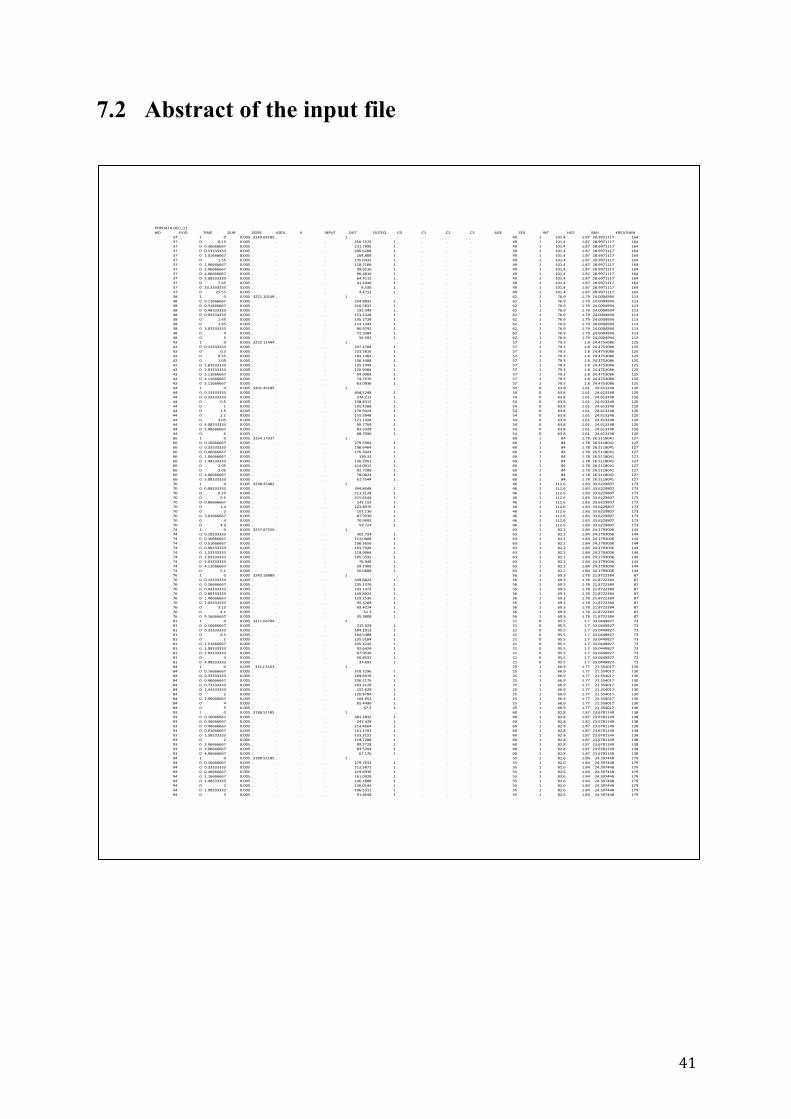
41

7.2 Abstract of the input file

POPDATADEC_11#ID EVID TIME DUR DOSE ADDL II INPUT OUT OUTEQ C0 C1 C2 C3 AGE SEX WT HGT BMI KREATININ

37 1 0 0.005 3149.69185 . . 1 . . . . . . 49 1 101.4 1.87 28.9971117 16437 0 0.15 0.005 . . . . 350.1576 1 . . . . 49 1 101.4 1.87 28.9971117 16437 0 0.36666667 0.005 . . . . 231.7896 1 . . . . 49 1 101.4 1.87 28.9971117 16437 0 0.53333333 0.005 . . . . 200.6208 1 . . . . 49 1 101.4 1.87 28.9971117 16437 0 1.01666667 0.005 . . . . 164.808 1 . . . . 49 1 101.4 1.87 28.9971117 16437 0 1.55 0.005 . . . . 135.0432 1 . . . . 49 1 101.4 1.87 28.9971117 16437 0 1.96666667 0.005 . . . . 118.2168 1 . . . . 49 1 101.4 1.87 28.9971117 16437 0 2.96666667 0.005 . . . . 99.9216 1 . . . . 49 1 101.4 1.87 28.9971117 16437 0 4.06666667 0.005 . . . . 80.4816 1 . . . . 49 1 101.4 1.87 28.9971117 16437 0 5.08333333 0.005 . . . . 64.4112 1 . . . . 49 1 101.4 1.87 28.9971117 16437 0 7.65 0.005 . . . . 41.1048 1 . . . . 49 1 101.4 1.87 28.9971117 16437 0 23.3333333 0.005 . . . . 4.536 1 . . . . 49 1 101.4 1.87 28.9971117 16437 0 23.55 0.005 . . . . 4.4712 1 . . . . 49 1 101.4 1.87 28.9971117 16438 1 0 0.005 3221.10148 . . 1 . . . . . . 62 1 76.9 1.79 24.0004994 11338 0 0.11666667 0.005 . . . . 294.8832 1 . . . . 62 1 76.9 1.79 24.0004994 11338 0 0.31666667 0.005 . . . . 216.5832 1 . . . . 62 1 76.9 1.79 24.0004994 11338 0 0.48333333 0.005 . . . . 192.348 1 . . . . 62 1 76.9 1.79 24.0004994 11338 0 0.93333333 0.005 . . . . 153.5328 1 . . . . 62 1 76.9 1.79 24.0004994 11338 0 1.45 0.005 . . . . 135.1728 1 . . . . 62 1 76.9 1.79 24.0004994 11338 0 1.95 0.005 . . . . 114.1344 1 . . . . 62 1 76.9 1.79 24.0004994 11338 0 3.03333333 0.005 . . . . 90.9792 1 . . . . 62 1 76.9 1.79 24.0004994 11338 0 4 0.005 . . . . 72.3384 1 . . . . 62 1 76.9 1.79 24.0004994 11338 0 5 0.005 . . . . 56.592 1 . . . . 62 1 76.9 1.79 24.0004994 11342 1 0 0.005 3232.12444 . . 1 . . . . . . 57 1 79.3 1.8 24.4753086 12542 0 0.13333333 0.005 . . . . 337.4784 1 . . . . 57 1 79.3 1.8 24.4753086 12542 0 0.3 0.005 . . . . 223.5816 1 . . . . 57 1 79.3 1.8 24.4753086 12542 0 0.55 0.005 . . . . 183.1464 1 . . . . 57 1 79.3 1.8 24.4753086 12542 0 1.05 0.005 . . . . 156.3408 1 . . . . 57 1 79.3 1.8 24.4753086 12542 0 1.63333333 0.005 . . . . 135.1944 1 . . . . 57 1 79.3 1.8 24.4753086 12542 0 2.03333333 0.005 . . . . 120.9384 1 . . . . 57 1 79.3 1.8 24.4753086 12542 0 3.11666667 0.005 . . . . 94.9968 1 . . . . 57 1 79.3 1.8 24.4753086 12542 0 4.11666667 0.005 . . . . 74.7576 1 . . . . 57 1 79.3 1.8 24.4753086 12542 0 5.11666667 0.005 . . . . 63.0936 1 . . . . 57 1 79.3 1.8 24.4753086 12544 1 0 0.005 3201.45185 . . 1 . . . . . . 54 0 63.8 1.61 24.613248 12044 0 0.13333333 0.005 . . . . 404.5248 1 . . . . 54 0 63.8 1.61 24.613248 12044 0 0.33333333 0.005 . . . . 274.212 1 . . . . 54 0 63.8 1.61 24.613248 12044 0 0.5 0.005 . . . . 238.8312 1 . . . . 54 0 63.8 1.61 24.613248 12044 0 1 0.005 . . . . 195.4368 1 . . . . 54 0 63.8 1.61 24.613248 12044 0 1.5 0.005 . . . . 170.9424 1 . . . . 54 0 63.8 1.61 24.613248 12044 0 2.1 0.005 . . . . 155.5848 1 . . . . 54 0 63.8 1.61 24.613248 12044 0 3.05 0.005 . . . . 121.1328 1 . . . . 54 0 63.8 1.61 24.613248 12044 0 4.08333333 0.005 . . . . 99.7704 1 . . . . 54 0 63.8 1.61 24.613248 12044 0 5.06666667 0.005 . . . . 83.3328 1 . . . . 54 0 63.8 1.61 24.613248 12044 0 6 0.005 . . . . 68.7096 1 . . . . 54 0 63.8 1.61 24.613248 12066 1 0 0.005 3254.17037 . . 1 . . . . . . 60 1 84 1.78 26.5118041 12766 0 0.16666667 0.005 . . . . 279.5904 1 . . . . 60 1 84 1.78 26.5118041 12766 0 0.33333333 0.005 . . . . 196.6464 1 . . . . 60 1 84 1.78 26.5118041 12766 0 0.46666667 0.005 . . . . 176.3424 1 . . . . 60 1 84 1.78 26.5118041 12766 0 1.06666667 0.005 . . . . 139.32 1 . . . . 60 1 84 1.78 26.5118041 12766 0 1.48333333 0.005 . . . . 126.2952 1 . . . . 60 1 84 1.78 26.5118041 12766 0 2.05 0.005 . . . . 114.0912 1 . . . . 60 1 84 1.78 26.5118041 12766 0 3.05 0.005 . . . . 92.7288 1 . . . . 60 1 84 1.78 26.5118041 12766 0 4.06666667 0.005 . . . . 78.0624 1 . . . . 60 1 84 1.78 26.5118041 12766 0 5.08333333 0.005 . . . . 61.7544 1 . . . . 60 1 84 1.78 26.5118041 12770 1 0 0.005 3238.35482 . . 1 . . . . . . 46 1 112.6 1.83 33.6229807 17370 0 0.08333333 0.005 . . . . 394.8048 1 . . . . 46 1 112.6 1.83 33.6229807 17370 0 0.25 0.005 . . . . 211.3128 1 . . . . 46 1 112.6 1.83 33.6229807 17370 0 0.5 0.005 . . . . 215.6544 1 . . . . 46 1 112.6 1.83 33.6229807 17370 0 0.86666667 0.005 . . . . 145.152 1 . . . . 46 1 112.6 1.83 33.6229807 17370 0 1.4 0.005 . . . . 123.8976 1 . . . . 46 1 112.6 1.83 33.6229807 17370 0 2 0.005 . . . . 107.136 1 . . . . 46 1 112.6 1.83 33.6229807 17370 0 3.01666667 0.005 . . . . 87.9336 1 . . . . 46 1 112.6 1.83 33.6229807 17370 0 4 0.005 . . . . 70.9992 1 . . . . 46 1 112.6 1.83 33.6229807 17370 0 4.9 0.005 . . . . 59.724 1 . . . . 46 1 112.6 1.83 33.6229807 17374 1 0 0.005 3237.87556 . . 1 . . . . . . 63 1 82.2 1.84 24.2793006 14474 0 0.18333333 0.005 . . . . 302.724 1 . . . . 63 1 82.2 1.84 24.2793006 14474 0 0.36666667 0.005 . . . . 213.0408 1 . . . . 63 1 82.2 1.84 24.2793006 14474 0 0.51666667 0.005 . . . . 196.3656 1 . . . . 63 1 82.2 1.84 24.2793006 14474 0 0.98333333 0.005 . . . . 163.7928 1 . . . . 63 1 82.2 1.84 24.2793006 14474 0 1.53333333 0.005 . . . . 119.9664 1 . . . . 63 1 82.2 1.84 24.2793006 14474 0 2.03333333 0.005 . . . . 105.5592 1 . . . . 63 1 82.2 1.84 24.2793006 14474 0 3.03333333 0.005 . . . . 78.948 1 . . . . 63 1 82.2 1.84 24.2793006 14474 0 4.11666667 0.005 . . . . 59.1408 1 . . . . 63 1 82.2 1.84 24.2793006 14474 0 5.1 0.005 . . . . 50.0688 1 . . . . 63 1 82.2 1.84 24.2793006 14476 1 0 0.005 3242.18889 . . 1 . . . . . . 56 1 69.3 1.78 21.8722384 8776 0 0.13333333 0.005 . . . . 349.6824 1 . . . . 56 1 69.3 1.78 21.8722384 8776 0 0.26666667 0.005 . . . . 235.1376 1 . . . . 56 1 69.3 1.78 21.8722384 8776 0 0.43333333 0.005 . . . . 193.1472 1 . . . . 56 1 69.3 1.78 21.8722384 8776 0 0.88333333 0.005 . . . . 149.8824 1 . . . . 56 1 69.3 1.78 21.8722384 8776 0 1.46666667 0.005 . . . . 119.2536 1 . . . . 56 1 69.3 1.78 21.8722384 8776 0 2.03333333 0.005 . . . . 95.3208 1 . . . . 56 1 69.3 1.78 21.8722384 8776 0 3.15 0.005 . . . . 69.4224 1 . . . . 56 1 69.3 1.78 21.8722384 8776 0 4.1 0.005 . . . . 51.3 1 . . . . 56 1 69.3 1.78 21.8722384 8776 0 5.16666667 0.005 . . . . 35.3808 1 . . . . 56 1 69.3 1.78 21.8722384 8781 1 0 0.005 3211.03704 . . 1 . . . . . . 21 0 95.5 1.7 33.0449827 7381 0 0.16666667 0.005 . . . . 215.028 1 . . . . 21 0 95.5 1.7 33.0449827 7381 0 0.33333333 0.005 . . . . 184.2912 1 . . . . 21 0 95.5 1.7 33.0449827 7381 0 0.5 0.005 . . . . 164.5488 1 . . . . 21 0 95.5 1.7 33.0449827 7381 0 1 0.005 . . . . 135.5184 1 . . . . 21 0 95.5 1.7 33.0449827 7381 0 1.51666667 0.005 . . . . 105.3216 1 . . . . 21 0 95.5 1.7 33.0449827 7381 0 1.98333333 0.005 . . . . 92.6424 1 . . . . 21 0 95.5 1.7 33.0449827 7381 0 2.93333333 0.005 . . . . 67.9536 1 . . . . 21 0 95.5 1.7 33.0449827 7381 0 4 0.005 . . . . 50.8032 1 . . . . 21 0 95.5 1.7 33.0449827 7381 0 4.98333333 0.005 . . . . 37.692 1 . . . . 21 0 95.5 1.7 33.0449827 7384 1 0 0.005 3211.5163 . . 1 . . . . . . 25 1 66.9 1.77 21.354017 13084 0 0.16666667 0.005 . . . . 318.7296 1 . . . . 25 1 66.9 1.77 21.354017 13084 0 0.33333333 0.005 . . . . 269.6976 1 . . . . 25 1 66.9 1.77 21.354017 13084 0 0.46666667 0.005 . . . . 236.2176 1 . . . . 25 1 66.9 1.77 21.354017 13084 0 0.73333333 0.005 . . . . 203.2128 1 . . . . 25 1 66.9 1.77 21.354017 13084 0 1.43333333 0.005 . . . . 155.628 1 . . . . 25 1 66.9 1.77 21.354017 13084 0 2 0.005 . . . . 126.8784 1 . . . . 25 1 66.9 1.77 21.354017 13084 0 2.96666667 0.005 . . . . 104.652 1 . . . . 25 1 66.9 1.77 21.354017 13084 0 4 0.005 . . . . 85.4496 1 . . . . 25 1 66.9 1.77 21.354017 13084 0 5 0.005 . . . . 67.5 1 . . . . 25 1 66.9 1.77 21.354017 13093 1 0 0.005 3188.51185 . . 1 . . . . . . 60 1 82.8 1.87 23.6781149 13893 0 0.16666667 0.005 . . . . 381.2832 1 . . . . 60 1 82.8 1.87 23.6781149 13893 0 0.36666667 0.005 . . . . 247.428 1 . . . . 60 1 82.8 1.87 23.6781149 13893 0 0.46666667 0.005 . . . . 214.4664 1 . . . . 60 1 82.8 1.87 23.6781149 13893 0 0.91666667 0.005 . . . . 161.1792 1 . . . . 60 1 82.8 1.87 23.6781149 13893 0 1.58333333 0.005 . . . . 133.3152 1 . . . . 60 1 82.8 1.87 23.6781149 13893 0 2 0.005 . . . . 119.7288 1 . . . . 60 1 82.8 1.87 23.6781149 13893 0 2.96666667 0.005 . . . . 89.2728 1 . . . . 60 1 82.8 1.87 23.6781149 13893 0 3.96666667 0.005 . . . . 83.5704 1 . . . . 60 1 82.8 1.87 23.6781149 13893 0 4.96666667 0.005 . . . . 67.176 1 . . . . 60 1 82.8 1.87 23.6781149 13894 1 0 0.005 3188.51185 . . 1 . . . . . . 55 1 82.6 1.84 24.397448 17994 0 0.16666667 0.005 . . . . 279.7632 1 . . . . 55 1 82.6 1.84 24.397448 17994 0 0.33333333 0.005 . . . . 212.5872 1 . . . . 55 1 82.6 1.84 24.397448 17994 0 0.46666667 0.005 . . . . 219.6936 1 . . . . 55 1 82.6 1.84 24.397448 17994 0 1.16666667 0.005 . . . . 161.0928 1 . . . . 55 1 82.6 1.84 24.397448 17994 0 1.48333333 0.005 . . . . 146.1888 1 . . . . 55 1 82.6 1.84 24.397448 17994 0 2 0.005 . . . . 126.0144 1 . . . . 55 1 82.6 1.84 24.397448 17994 0 2.98333333 0.005 . . . . 106.5312 1 . . . . 55 1 82.6 1.84 24.397448 17994 0 4 0.005 . . . . 91.8648 1 . . . . 55 1 82.6 1.84 24.397448 179

42

7.3 The model file

#PRICL0,1,10V0,0.1,20Vp0,1,25Q0,1,50

#COVAGESEXWTHGTBMIKREATININ

#SecWTc=WT/72BMIc=BMI/25KREATININc=KREATININ/60+IF (SEX.GT.0)KREATININc=KREATININ/45CL=CL0*WTc**0.75V=V0Vp=Vp0*WTcQ=Q0*WTc**0.75Ke=CL/VKCP=Q/VKPC=Q/Vp

#OutY(1) = X(1)/V

#ERRL=10.1523073,0.01747435,-0.000003919581,0