Mean velocity and temperature profiles in a sheared diabatic turbulentboundary layerDan Li, Gabriel G. Katul, and Elie Bou-Zeid Citation: Phys. Fluids 24, 105105 (2012); doi: 10.1063/1.4757660 View online: http://dx.doi.org/10.1063/1.4757660 View Table of Contents: http://pof.aip.org/resource/1/PHFLE6/v24/i10 Published by the American Institute of Physics. Related ArticlesIonization and hydrolysis of dinitrogen pentoxide in low-temperature solids Low Temp. Phys. 27, 890 (2001) Spectral scaling of static pressure fluctuations in the atmospheric surface layer: The interaction between largeand small scales Phys. Fluids 10, 1725 (1998) On the dynamics of strong temperature disturbances in the upper atmosphere of the Earth Phys. Fluids A 1, 887 (1989) Frequency response of cold wires used for atmospheric turbulence measurements in the marine environment Rev. Sci. Instrum. 50, 1463 (1979) Stability of rectilinear geostrophic vortices in stationary equilibrium Phys. Fluids 19, 929 (1976) Additional information on Phys. FluidsJournal Homepage: http://pof.aip.org/ Journal Information: http://pof.aip.org/about/about_the_journal Top downloads: http://pof.aip.org/features/most_downloaded Information for Authors: http://pof.aip.org/authors

Downloaded 16 Oct 2012 to 152.3.110.48. Redistribution subject to AIP license or copyright; see http://pof.aip.org/about/rights_and_permissions

PHYSICS OF FLUIDS 24, 105105 (2012)

Mean velocity and temperature profiles in a sheareddiabatic turbulent boundary layer

Dan Li,1,a) Gabriel G. Katul,2 and Elie Bou-Zeid1

1Department of Civil and Environmental Engineering, Princeton University, Princeton,New Jersey 08544, USA2Nicholas School of the Environment, Box 80328, Duke University, Durham,North Carolina 27708, USA and Department of Civil and Environmental Engineering,Duke University, Durham, North Carolina 27708, USA

(Received 18 March 2012; accepted 7 September 2012; published online 16 October 2012)

In the atmospheric surface layer, modifications to the logarithmic mean velocity andair temperature profiles induced by thermal stratification or convection are accountedfor via stability correction functions φm and φh, respectively, that vary with thestability parameter ς . These two stability correction functions are presumed to beuniversal in shape and independent of the surface characteristics. To date, there isno phenomenological theory that explains all the scaling laws in φh with ς , how φh

relates to φm, and why φh ≤ φm is consistently reported. To develop such a theory,the recently proposed links between the mean velocity profile and the Kolmogorovspectrum of turbulence, which were previously modified to account for the effects ofbuoyancy, are generalized here to include the mean air temperature profile. The result-ing theory explains the observed scaling laws in φm and φh reported in many field andnumerical experiments, predicts their behaviors across a wide range of atmosphericstability conditions, and elucidates why heat is transported more efficiently thanmomentum in certain stability regimes. In particular, it is shown that the enhance-ment in heat transport under unstable conditions is linked to a “scale-resonance”between turnover eddies and excursions in the instantaneous air temperature pro-files. Excluding this scale-resonance results in the conventional Reynolds analogywith φm = φh across all stability conditions. C© 2012 American Institute of Physics.[http://dx.doi.org/10.1063/1.4757660]

I. INTRODUCTION

The mean velocity and air temperature profiles in sheared diabatic boundary layers are affectedby both shear and buoyant forces. In the atmospheric surface layer (ASL), for example, the effects ofbuoyancy resulting from surface cooling or heating can be more significant than shear in determiningthe dynamics of the turbulent kinetic energy (TKE). According to Monin-Obukhov Similarity Theory(MOST),1–3 buoyancy distorts the logarithmic shape of the mean velocity and air temperature profilesvia “universal” stability correction functions φm and φh, defined for the ASL as3

du

dz

κvz

u∗= φm (ς ) , (1)

dT

dz

κvz

T∗= φh (ς ) , (2)

where u is the longitudinal velocity, T is the air temperature, u∗ = √τo/ρ is the friction velocity, τ o

is the surface shear stress, ρ is the mean air density, T∗ = −w′T ′/u∗ is the surface temperature scale,

a)Author to whom correspondence should be addressed. Electronic mail: danl@princeton.edu. Telephone: 609-933-4802.

1070-6631/2012/24(10)/105105/16/$30.00 C©2012 American Institute of Physics24, 105105-1

Downloaded 16 Oct 2012 to 152.3.110.48. Redistribution subject to AIP license or copyright; see http://pof.aip.org/about/rights_and_permissions

105105-2 Li, Katul, and Bou-Zeid Phys. Fluids 24, 105105 (2012)

w′T ′ = Hs/ρC p is the kinematic sensible heat flux density, w is the vertical velocity, κv (= 0.40)is the von Karman constant, z is the height above the ground surface, ς = z/L is the atmospheric

stability parameter, L is the Obukhov length L = −u3∗/(

κv

g

Tw′T ′

)(neglecting the effect of water

vapor on density), g (= 9.81 m s−2) is the gravitational acceleration, and Cp is the specific heatcapacity of dry air at constant pressure. The overbar indicates Reynolds-averaged values and theprimes denote turbulent excursions from them. These stability correction functions are widely usedin hydrological, ecological, and atmospheric studies because they explicitly show how variationsin atmospheric stability modify the relationship between turbulent fluxes and mean gradients. Theyare also critical in numerical models of the lower atmosphere since they are the basis of multipleturbulence closure schemes that are used in climate and weather simulations.1, 3, 4

For neutral atmospheric stability conditions (i.e., ς = 0), setting φm(0) = 1 and φh(0) = 1 (or anyother constant3) recovers the canonical logarithmic profile shapes for mean velocity and temperature.It is for this reason that φm and φh are labeled as stability correction functions: they modify thelogarithmic profiles as atmospheric stability changes due to surface heating or cooling. In “idealizedmicro-meteorological conditions” that are associated with flows that are stationary and planar-homogeneous, with very high Reynolds number, zero mean vertical velocity and pressure gradients,and no Coriolis effects, these stability corrections are assumed to be “universally” independent ofsurface properties or other boundary conditions except through their effect on the surface fluxes andthus L. As argued in the original work of Monin and Obukhov,2 the precise form of φm and φh canbe inferred from experiments.

Since their seminal 1954 publication, many such experiments have been conducted to determinethe shapes of φm and φh. The functions inferred from the “weighty” Kansas experiments, commonlyreferred to as the Businger-Dyer (BD) relations,5 are the corner-stone of micro-meteorology. Manynumerical studies, including higher-order closure modeling6 and large eddy simulations7 (awayfrom the wall-modeled region where the φm and φh need to be imposed), also agree with the BDformulation for φm and φh, at least for the range of ς reported in the original Kansas experiments.Table I summarizes many empirically fitted functions for φm and φh reported in the literature,including those of BD,5 Hogstrom,8 Wilson,9 Kader and Yaglom,10 and Brutsaert.1 Fig. 1 illustrateshow some reported φm and φh, as well as the model calculations of Vila-Guerau de Arellano et al.6

(hereinafter VDZ95), vary with ς . While disagreement among these studies can be noted as to the

TABLE I. Stability correction functions for velocity and temperature.

φm φh

Unstable conditionsBusinger-Dyer φm(ς ) = (1 − 15ς )−1/4 φh(ς ) = 0.74(1 − 9ς )−1/2

Hogstroma φm(ς ) = (1 − 19.3ς )−1/4 φh(ς ) = (1 − 12ς )−1/2

Wilson φm(ς ) = (1 + 3.6|ς |2/3)−1/2 φh(ς ) = (1 + 7.9|ς |2/3)−1/2

Kader and Yaglomb φm (ς ) =⎧⎨⎩

1.04 0 < −ς ≤ 0.10.50 (−ς)−1/3 0.3 ≤ −ς ≤ 30.21 (−ς)1/3 −ς ≥ 5

φh (ς ) =⎧⎨⎩

0.96 0 < −ς ≤ 0.10.32 (−ς)−1/3 0.3 ≤ −ς ≤ 30.27 (−ς)−1/3 −ς ≥ 5

Brutsaert φm (ς ) =⎧⎨⎩

0.33 + 0.41 |ς |4/3

0.33 + |ς | 0 < −ς ≤ 14.5

1 − ς > 14.5φh (ς ) = 0.33 + 0.057 |ς |0.78

0.33 + |ς |0.78

Stable conditionsBusinger-Dyer φm(ς ) = 1 + 4.7ς φh(ς ) = 0.74 + 4.7ς

Hogstrom φm(ς ) = 1 + 4.8ς φh(ς ) = 1 + 7.8ς

Brutsaert φm (ς ) ={

1 + 5ς 0 < ς ≤ 16 ς > 1

φh (ς ) ={

1 + 5ς 0 < ς ≤ 16 ς > 1

aSee a review of different stability corrections in Tables VI and VII in Hogstrom.8bIn Kader and Yaglom,10 the von-Karman constant was not included in the definitions of L, φm, and φh. Here, the von-Karmanconstant κv = 0.40 is added and thus the coefficients reported here differ from those listed in their original work.

Downloaded 16 Oct 2012 to 152.3.110.48. Redistribution subject to AIP license or copyright; see http://pof.aip.org/about/rights_and_permissions

105105-3 Li, Katul, and Bou-Zeid Phys. Fluids 24, 105105 (2012)

10−2

100

102

10−2

10−1

100

−ζφ m

−1/4

−1/3Businger−DyerHogstromWilsonVDZ95

10−2

100

102

10−2

10−1

100

−ζ (unstable)

φ h

−1/2

−1/3

0 1 21

3

5

7

9

11

ζ

φ m

0 1 21

3

5

7

9

11

ζ (stable)

φ hFIG. 1. Stability correction functions for the mean velocity and air temperature under unstable and stable conditions. Underunstable conditions, log-log scales are used to emphasize scaling laws; while under stable conditions, linear axes are used.The functions are as listed in Table I.

exact values of the coefficients in the functions under a given stability regime, it is evident fromFig. 1 that all studies agree that φm �= φh when ς < 0. Under neutral and stable conditions (ς ≥ 0),nonetheless, some studies support φm = φh but others do not. Some of the scaling laws appear welldocumented and consistent across all these studies. For example, φm and φh increase linearly withincreasing ς under stable conditions in all the functions shown in Fig. 1. Under moderately unstableconditions (roughly when 1 < −ς < 5), the scaling laws in the BD relations appear to followφm ∼ (− ς )−1/4 and φh ∼ (−ς )−1/2. While the free-convection limit is rarely achieved in ASLstudies for the idealized micrometeorological conditions (ς > >1), φm and φh are expected to scaleas (−ς )−1/3 due to the fact that the effects of u* cannot be dynamically significant and only the(−ς )−1/3 scaling “cancels out” the u* dependence when ς > >1. Although these scaling laws arewell established and have been confirmed by a large number of experiments, model calculations,and large eddy simulations, there is no phenomenological theory to explain their onset. In addition,the causes as to why the scaling laws of φm and φh with stability are different for ς < 0, but not forς > 0, have resisted complete theoretical treatment to date.

Recently, a phenomenological approach was proposed to link the mean velocity profile tothe turbulent energy spectrum.11 The model was then extended to include the effects of thermalstratification on the mean turbulent kinetic energy dissipation rate (= ε) and the eddy-size anisotropy,and consequently on φm(ς ), as discussed in Ref. 12. This approach is expanded here to include bothmomentum and temperature, with a focus on the onset of dissimilarity between momentum and heatacross certain stability regimes. By expanding this approach, it is found that interactions betweenthe velocity of turnover eddy and excursions in the instantaneous air temperature profile cannotbe ignored as implicitly assumed for the velocity profile, thereby requiring the introduction of anew length scale characterizing the strength of this interaction. This length scale must be explicitlyaccounted for to successfully recover the stability correction functions for temperature as well as thedissimilarity between momentum and temperature (φm �= φh) for ς < 0.

II. THEORY

The mean longitudinal momentum balance and the mean temperature budget for the “ideal-ized micro-meteorological conditions” previously discussed reduce to3 ∂w′T ′/∂z = ∂u′w′/∂z = 0.Upon integration with respect to z, these equations result in turbulent shear stress and heat flux near

Downloaded 16 Oct 2012 to 152.3.110.48. Redistribution subject to AIP license or copyright; see http://pof.aip.org/about/rights_and_permissions

105105-4 Li, Katul, and Bou-Zeid Phys. Fluids 24, 105105 (2012)

FIG. 2. Turbulent momentum and sensible heat fluxes due to the turnover of an isotropic eddy of radius s acting on a meanvelocity and temperature profiles as in Gioia et al.11 and Katul et al.12 The isotropic eddy transfers momentum down at arate ρu (z + s) v (s) and up at a rate ρu (z − s) v (s); similarly, it transfers heat down at a rate ρT (z + s) v (s) and up at arate ρT (z − s) v (s) when the sensible heat flux Hs > 0. In Gioia et al.,11 it was argued that the most efficient eddy sizethat transports momentum to the ground (and hence, by extension, heat from/to the ground) is an eddy of size s = z. Katulet al.12 extended the Gioia et al.11 model to thermally stratified conditions. An addition to the Katul et al.12 model is theconsideration of the mean temperature profile in this paper.

the ground (but above the buffer layer) identical to their counterparts at an arbitrary height z wellabove the surface. Extension into the viscous and buffer layers can show that the sum of viscous andturbulent fluxes is constant. Hence u′w′ and w′T ′ well above the surface are equal to the surfacefluxes. These idealized simplifications apply in the so-called log-region of a sheared boundary layer3

(i.e., the ASL, or the bottom 10%–20% of the atmospheric boundary layer) and imply that L does notvary with z in this region. According to the Gioia et al.11 model illustrated in Fig. 2, the momentumfluxes can be expressed as

u2∗ = αmv (s) [u (z + s) − u (z − s)] ≈ αmv (s)

[du (z)

dz2s

]. (3)

A straightforward extension to the sensible heat fluxes yields

w′T ′ = −αhv (s)[T (z + s) − T (z − s)

] ≈ −αhv (s)

[dT (z)

dz2s

], (4)

where v (s) = w21/2

is the root mean square of the difference in vertical velocity at the edge andat the center of an isotropic turnover eddy of size s depicted in Fig. 2; u (z + s) − u (z − s) is thenet kinematic momentum, per unit velocity of the turnover eddy, exchanged between z + s andz – s due to eddies of radius s; similarly, T (z + s) − T (z − s) is the net kinematic heat flux, per unitvelocity of the turnover eddy, exchanged at height z; and αm and αh are proportionality constants.

Similar to Gioia et al.,11 a logical starting point is to assume that eddies that contribute mostefficiently to momentum and heat transport are those attached eddies that directly “touch” the surface.Consequently, these “attached-eddies” are of size s = z, and Eqs. (3) and (4) reduce to

2αm

κv

v (z)

u∗

[du (z)

dz

κvz

u∗

]= 2

αm

κv

v (z)

u∗[φm] = 1, (5)

2αh

κv

v (z)

u∗

[dT (z)

dz

kvz

T∗

]= 2

αh

κv

v (z)

u∗[φh] = 1. (6)

Plausible solutions to Eqs. (5) and (6) must satisfy αmφm = αhφh. If φm(0) = φh(0) = 1 underneutral conditions, αm must be identical to αh, which further leads to φm = φh under all stabilityconditions. A consequence of this finding is that when the phenomenological model in Gioia et al.11

is extended to air temperature with no other modification, it will result in complete similarity between

Downloaded 16 Oct 2012 to 152.3.110.48. Redistribution subject to AIP license or copyright; see http://pof.aip.org/about/rights_and_permissions

105105-5 Li, Katul, and Bou-Zeid Phys. Fluids 24, 105105 (2012)

momentum and heat transport, i.e., the Reynolds analogy. As earlier noted in Table I, there is someevidence supporting the Reynolds analogy under near-neutral and stable conditions; however, thefact that this phenomenological model does not produce the observed dissimilarity between φm andφh under unstable conditions13, 14 motivates new refinements. In addition, this shortcoming of themodel extension cannot be overcome by simply allowing φm(0) �= φh(0) as in some studies listed inTable I since that only results in a constant ratio of the two functions under all values of ς . Thus,dissimilarity between momentum and heat for near-neutral conditions alone cannot alter the scalinglaws of φm and φh with ς .

The solution to Eq. (5) under thermally stratified conditions is given in Ref. 12 and only the mainsteps leading to the final results are reviewed for completeness. First, Katul et al.12 estimated v (z)from the Kolmogorov theory for locally homogeneous and isotropic turbulence as v (z) = [kεε z]1/3,where kε = 4/5, and ε is the mean TKE dissipation rate. This theory provides a link between v (z)and z1/3, but its implementation requires an estimate of ε. Such an estimate can be obtained from theturbulent kinetic energy budget equation subjected to the same idealizations as the mean longitudinalmomentum balance and the mean air temperature budget equation. Moreover, these idealizationsare complemented by a further assumption that the sum of the pressure transport and flux transportterms is negligible relative to the other terms (this requirement is partially relaxed later though).Hence,3

ε = u2∗∂ u

∂z+ g

T

Hs

ρC p+(

−∂w′e2

∂z− 1

ρ

∂w′ p′

∂z

)≈ u2

∗∂ u

∂z+ g

T

Hs

ρC p= u3

∗κvz

(φm − ς ) , (7)

where e2 = 0.5(u′2 + v′2 + w′2) is the instantaneous TKE and p′ is the turbulent pressure.

Note that under neutral conditions, ς = 0, φm(0) = 1, thus v (z) = [kεε z]1/3 = [kεzu3∗/κvz]1/3

= [kε/κv]1/3u∗ ≈ 1.26u∗, which is consistent with Townsend’s attached-eddy hypothesis15 that ed-dies attached to the wall scale with z and have u* as their characteristic velocity (see Smits et al.16 fora recent comprehensive discussion). Moreover, this value of v (z) ≈ 1.26u* is commensurate with

the value of w′21/2for near-neutral conditions,3 as expected when it is this velocity of the turnover

eddy that contributes to vertical momentum and heat exchange rates.With this expression of ε, substituting v (z) into Eqs. (5) and (6) yields the O’KEYPS equations:17

23α3m kε

κ4v

[φm (ς )]4

[1 − ς

φm (ς )

]= 1, (8)

23α3h kε

κ4v

[φh (ς )]3 φm (ς )

[1 − ς

φm (ς )

]= 1. (9)

Upon imposing φm(0) =φh(0) = 1 under neutral conditions, these equations result in 23α3m kε/κ

4v = 1

and 23α3h kε/κ

4v = 1, thus αm = αh = (

κ4v /23 kε

)1/3 ≈ 0.21. As noted in Katul et al.,12 Eq. (8)recovers the –1/4 power-law for small −ς , the –1/3 power-law for large −ς , and the proportionalincrease in φm with an increasing ς > 0. However, Eq. (8) does not produce the correct shapes ofφm, which, according to Katul et al.,12 is attributed to (1) finite contributions from the turbulent fluxtransport of kinetic energy and pressure transport terms in the TKE budget, and (2) more importantly,the anisotropy of the attached eddy in the longitudinal direction due to thermal stratification thatresults in some departure from the Kolmogorov scaling. After including these two effects, it wasshown in Katul et al.12 that Eq. (8) is changed into

[φm]4

[(1 − (1 + β)

ς

φm

)]= 1

fw (ς ), (10)

where β =(

−∂w′e2

∂z− 1

ρ

∂w′ p′

∂z

)/

(g

T

Hs

ρC p

)is a measure of the contribution from the two

transport terms in parenthesis in Eq. (7), which now results in ε = u3∗

κvz(φm − (1 + β) ς). The

Downloaded 16 Oct 2012 to 152.3.110.48. Redistribution subject to AIP license or copyright; see http://pof.aip.org/about/rights_and_permissions

105105-6 Li, Katul, and Bou-Zeid Phys. Fluids 24, 105105 (2012)

function fw (ς ) = [v (z) / (kεε z)1/3

]3is an estimate of the effect of thermal stratification on the

aspect ratio of the turnover eddy since v (z) = (kεε z fw (ς ))1/3. With an estimate of fw (ς ) basedon how the peak of the vertical velocity spectra changes relative to its near-neutral counterpart andsetting β to unity (an upper limit in the Kansas experiment), Eq. (10) successfully recovered thecorrect shape of φm. The fact that φm is sensitive to fw (ς ) but not to β, as reported in Katul et al.,12

implies that thermal stratification primarily modulates momentum transport through a change in theaspect ratio of the turnover eddy.

In summary, the model in Katul et al.12 only modifies v (z) compared to the phenomenologicalmodel in Gioia et al.11 Since the resulting equation αmφm = αhφh from Eqs. (5) and (6) is independentof v (z), it is clear that a direct extension of the model in Katul et al.12 cannot explain the dissimilarityof φm and φh under unstable conditions. As such, in addition to the thermal stratification effect onthe TKE budget and the eddy aspect ratio, a new mechanism must become significant in the heattransport under unstable conditions, while being suppressed or reduced under stable conditions, toaccount for such dissimilarity.

III. THE ROOTS OF THE DISSIMILARITY BETWEEN φm AND φh

Section I highlighted differences in the observed scaling laws for φh compared to φm undermoderately unstable conditions, as well as differences in the magnitude of these two functionsunder all unstable conditions. Straightforward extension of previous models did not capture thesedifferences. In this section, the physical basis of these differences is identified so that it can beincorporated in a generalized phenomenological model for both φm and φh.

Equations (3) and (4) postulate that a turnover eddy is passively acting on the “time-averaged”velocity and air temperature profiles, which are smooth and steady. A generalized phenomenologicalmodel would relax this assumption starting with the following hypothesis: across the turnovereddy, the spatial excursions embedded in “instantaneous” velocity and temperature profiles couldinteract with the turnover velocity thereby creating additional “dispersive fluxes” (Fig. 3). Thus,Eqs. (3) and (4) are first reformulated as

u2∗ = αm 〈vu〉 = αm (〈v〉 〈u〉+ 〈vu〉) = αm (〈v〉 [u (z + s) − u (z − s)] +Rvuσvσu) ,

(11)

H

ρC p=−αh 〈vT 〉=−αh

(〈v〉 〈T 〉+ ⟨vT

⟩)=−αh (〈v〉 [T (z+s) − T (z − s)] +RvT σvσT ) ,

(12)

FIG. 3. Turnover-eddy scale dominating case (a) and turnover-eddy scale interacting with fluctuations in the instantaneoustemperature-gradient case (b). In (a), the vertical profile of temperature (only temperature is shown here but this argumentalso holds for velocity) is smooth across the turnover eddy size and the characteristic length scale of temperature is too largeto be important; in (b), the vertical profile of temperature is fluctuating so that the characteristic length scale of temperatureis reduced and becomes comparable in magnitude to the turnover eddy size. Note that case (b) generates a smaller gradientlength scale than case (a).

Downloaded 16 Oct 2012 to 152.3.110.48. Redistribution subject to AIP license or copyright; see http://pof.aip.org/about/rights_and_permissions

105105-7 Li, Katul, and Bou-Zeid Phys. Fluids 24, 105105 (2012)

where u and T are variations in the vertical profiles across the turnover eddy (i.e., from z – s to z+ s); v is the velocity of turnover eddy; brackets denote spatial averaging across the turnover eddyand the tilde indicates excursions from the spatial mean. The Rvu and RvT are spatial correlationcoefficients that account for any interactions between the turnover velocity and excursions in theinstantaneous velocity/temperature profiles across the turnover eddy, while σ denotes the standarddeviation of a parameter. When the scales modulating v (= Lv) and u(= Lu) are sufficientlyseparated, Rvu ≈ 0 and the previous phenomenological theory in Eq. (3) is recovered. This scaleseparation is likely for momentum since the mean velocity varies over length scales commensuratewith z, while the velocity of the turnover eddy varies over length scales commensurate to z1/3.Hence, even a 50% difference between v and u can result in an order of magnitude separationbetween in Lv and Lu. However, when these length scales are comparable, we expect a “boost” inoverall fluxes due to interactions (i.e., Rvu and RvT), which were not considered in the originalphenomenological model.

This dispersive boost hypothesis is also supported by a complimentary analysis detailed inAppendix A where, starting from momentum and sensible heat flux budgets, it is demonstratedthat the sensible heat flux might be significantly increased by the dynamic role of temperaturevariance σ 2

T (Eq. (A8)), which can be associated with the excursions in the temperature profiles.As in Eqs. (11) and (12), this boost appears as an “additive term” to the momentum and sensibleheat fluxes resulting from the interaction between the turnover eddy and the instantaneous verticalprofiles. We point out the striking similarity between Eqs. (11) and (12) and the final equations inAppendix A (e.g., Eqs. (A7) and (A8)) and emphasize that both arguments suggest that there is amissing contribution in the original model. This contribution is associated with excursions in thevelocity/temperature profiles across the turnover eddy and their interactions with the turnover eddy.

From a phenomenological perspective, the original models assume that the only length scalecontrolling the flux-generation process is s = fw (ς ) z, where fw = 1 in Gioia et al.11 and fw changeswith stability in Katul et al.12 This can only be true when the size of the turnover eddy is muchsmaller than the characteristic length scale of the velocity or temperature profiles, and thus it solelycontrols the interactions between the turnover eddy and these profiles (Fig. 3(a)). When buoyancystarts to become important in turbulence generation however, this scale separation is likely to beviolated for temperature in certain stability regimes due to possible scale-resonance between theturnover eddy, the mean temperature profile (Fig. 3(b)), and temperature fluctuations (surrogated toa length scale impacting σ T as shown in Appendix A) embedded within the instantaneous profiles.One possible and measurable indicator of such a scale-resonance effect between the turnover velocityfield and the temperature field is the ratio of integral time scales of the turnover velocity and thetemperature. The integral time scale of the vertical velocity measures the temporal coherence ofthe turnover eddy (similar to the scale at which the vertical velocity spectra peak, which was usedin Katul et al.12), while the integral time scale of the temperature fluctuations indicates coherencewithin the temperature fluctuations. These time scales are often interpreted as horizontal integrallength scales when employing Taylor’s frozen turbulence hypothesis. While distortions to theseintegral scale estimates are expected due to the use of Taylor’s hypothesis (especially with changesin ς ), these distortions are likely to have a weaker impact on the ratio of these length scales, andthus, discussing these ratios is preferred.

Although these horizontal scales are not direct indicators of the characteristic scales of veloc-ity/temperature variations in the vertical direction (i.e., the scales over which u(z + s) − u(z − s)and T(z + s) − T(z − s) vary), spanwise vorticity near the surface (consistent with the turnovereddy model) will act to rotate vertical structures into a horizontal position and induce a correlationbetween vertical and horizontal integral scales, as shown in Fig. 3. Here, we assume that the ratiosof integral scales for w, u, and T in the horizontal direction (as inferred from Taylor’s hypothesis),when close to unity,can indicate a scale-resonance potential. In the following part, two data setscollected in the ASL over a lake and a glacier are used to calculate the integral length scales of w,u, and T in the streamwise direction. Details about the two data sets, quality control measures, andcalculations of the stability parameter can be found in Vercauteren et al.,18 Bou-Zeid et al.,14, 19 andLi et al.20 The integral length scales are calculated by integrating the autocorrelation functions upto their first zero-crossings and invoking Taylor’s hypothesis.3 The lake data set covers unstable to

Downloaded 16 Oct 2012 to 152.3.110.48. Redistribution subject to AIP license or copyright; see http://pof.aip.org/about/rights_and_permissions

105105-8 Li, Katul, and Bou-Zeid Phys. Fluids 24, 105105 (2012)

10−1

100

101

ζ (stable)

IT / I

w

Iu / I

w

10−2

10−1

100

101

100

101

102

−ζ (unstable)

Rat

ios

of in

tegr

al le

ngth

sca

les

FIG. 4. Ratios of the integral length scale of the steamwise velocity/temperature to that of the turnover velocity.

slightly stable conditions and the glacier data set covers slightly stable to very stable conditions sothat the combination of two data sets provides a complete picture of scale-resonance between theturnover eddy and the vertical profiles of mean velocity/temperature over a wide range of stabilityregimes.20

As shown in Fig. 4, the ratio of integral length scales of the longitudinal velocity and the turnovervelocity (Iu/Iw) is on the order of 10–100 for all ς so that interactions between the turnover velocityand the velocity gradients across the eddy remain largely controlled by the scale of the turnovervelocity. The fact that a large scale-separation exists between the mean velocity and the turnovervelocity under all stability conditions implies that thermal stratification affects momentum transportby means of modifying the turnover eddy only, as postulated in Katul et al.12

Similarly, it is clear that under near-neutral and stable conditions, the ratios of the integral lengthscales of the temperature and the turnover velocity (IT/Iw) are much larger than unity. However, asthe instability increases, the ratio IT/Iw decreases to order unity when –z/L > 0.2, implying thatscale separation is significantly reduced. A possible contributing mechanism to this reduction inscale-separation is the increase in Iw under unstable conditions observed when buoyancy contributesto the generation of eddies.12, 21 But it is the decrease in the integral length scale of temperaturewhen –z/L > 0.2 that turns out to be more important in reducing the scale-separation (not directlyshown here but can be inferred from Fig. 4). Consequently, the interactions of the turnover eddy withthe mean as well as with the instantaneous temperature profile jointly contribute to heat transport.As the atmosphere becomes more unstable, the scale-resonance between the turnover velocityand the temperature fluctuations is enhanced and violates the implicit assumption in the originalphenomenological model.

IV. GENERALIZING THE PHENOMENOLOGICAL MODEL

To include the possible effect of scale-resonance between the turnover velocity and temperatureexcursions and to provide a complete framework for studying stability correction functions forboth momentum and temperature, new scales that characterize the variability in these verticalprofiles, fu(ς ) and fT(ς ), are hence needed in the model. With (du(z)/dz) 2s = (du(z)/dz) z fu (ς )and

(dT (z)/dz

)2s = (

dT (z)/dz)

z fT (ς ) substituted into Eqs. (3) and (4), we obtain

u2∗ = αm (kεε z fw (ς ))1/3

[du (z)

dzz fu (ς )

], (13)

w′T ′ = −αh (kεε z fw (ς ))1/3

[dT (z)

dzz fT (ς )

]. (14)

Downloaded 16 Oct 2012 to 152.3.110.48. Redistribution subject to AIP license or copyright; see http://pof.aip.org/about/rights_and_permissions

105105-9 Li, Katul, and Bou-Zeid Phys. Fluids 24, 105105 (2012)

Equations (13) and (14), together with ε = u3∗

κvz(φm − (1 + β) ς ) and the definitions of φm and φh,

lead to

[φm]4

[(1 − (1 + β)

ς

φm

)]= 1

fw (ς )

1

( fu (ς ))3 , (15)

[φh]3 φm

[(1 − (1 + β)

ς

φm

)]= 1

fw (ς )

1

( fT (ς ))3 . (16)

Another theoretical approach leading to a formulation similar to Eq. (16) is presented in Appendix Bbased on the Kolmogorov theory22 for the velocity spectrum and the Kolmogorov-Corrsin theory22, 23

for the temperature fluctuation spectrum. The new derivation presented in Appendix B also arguesthat the heat flux is generated through interactions between the turnover velocity and “macro-scale”

variations in the instantaneous temperature profile (= T ′2 (s)1/2

) when s = z, with T ′2 (z)1/2

beingproportional to T (z + s) − T (z − s). This approach predicts that φh differs from φm partly due todifferences in integral length scales (IT /Iw �= Iu/Iw) and intermittency parameters, which are largerfor heat than horizontal velocity in the inertial subrange because of “contamination” due to prevalentramp structures dominating the temperature time series.24

To solve Eqs. (15) and (16), expressions for fw, fT, and fu are required. An estimate of fw (ς ) isalready given in Katul et al.12 based on an interpolation of the functions presented in Kaimal andFinnigan21 for the spectral peaks in the vertical velocity derived from the Kansas experiment. Theinterpolated fw (ς ) is slightly revised in this study compared to the function given in Katul et al.12

to ensure that φmscales linearly with ς under all stable conditions, which according to Eq. (15)requires fw (ς ) ∼ ς−4, yet ensuring the smoothness of the function fw at ς = 0. ComparingEqs. (15) and (16) to Eqs. (11) and (12), respectively, reveals that fu and fT act like “amplificationfactors” that account for interactions between the turnover eddy and the excursions in the verticalprofiles. Due to the scale separation between the turnover velocity and the characteristic length scalefor the velocity profile (Fig. 4), we use fu(ς ) = 1 under all stability conditions. Through similarreasoning, we use fT(ς ) = 1 under neutral and stable conditions; while under unstable conditions, fTincreases gradually in accordance with Fig. 4 to represent the scale-resonance between the turnovereddy and the temperature gradients. In addition, fT approaches fw asymptotically as instabilityincreases. This follows from the fact that the ratio of horizontal integral length scales of the verticalvelocity and temperature, which is used as an estimate of the ratio of the characteristic length scales ofthe turnover eddy and the temperature gradients, approaches unity gradually as instability increases,as shown in Fig. 4. The fact that the characteristic length scale of the temperature gradients becomesimportant gradually (ratio of the integral scale decreases smoothly in Fig. 4) indicates that fT shouldincrease more slowly than fw. It also needs to be pointed that the increase in fT is mainly in the range−5 < ς < −0.2; this is related to the significant reduction in the scale-separation in this regime asshown in Fig. 4. It turns out that it is the rapid increase of fT in this range of ς , compared to fu thatresults in different scaling laws for temperature, (− ς )−1/2, when compared to momentum, (−ς )−1/4.From these theoretical and observational constraints, a function form for fT can be inferred.

The final expression of fw, fT and fu are as follows (Fig. 5):

fw(ς ) =

⎧⎪⎪⎪⎨⎪⎪⎪⎩1 − 0.38

0.55

[1 − exp(25ς )

]ς ≤ 0(

1 + 25

4

0.38

0.55ς

)−4

ς > 0

, (17)

fT (ς ) =

⎧⎪⎪⎨⎪⎪⎩(

1 + 10.5 |ς |1.5

1 + 0.3 |ς |1.5

)1/3

ς ≤ 0

1 ς > 0

, (18)

Downloaded 16 Oct 2012 to 152.3.110.48. Redistribution subject to AIP license or copyright; see http://pof.aip.org/about/rights_and_permissions

105105-10 Li, Katul, and Bou-Zeid Phys. Fluids 24, 105105 (2012)

−10 −8 −6 −4 −2 0 20

1

2

3

4

ζA

niso

trop

y fu

nctio

ns

f

w

fT

fu

−1 0 101234

FIG. 5. The anisotropy functions used to recover the stability correction functions. For mean velocity, u, the anisotropyfunction remains unity due to the large scale-separation between the characteristic length scale of a turnover eddy and thecharacteristic length scale of the mean velocity field. So does the anisotropy function for temperature under neutral andstable conditions. However, as instability increase, the anisotropy function for temperature increases in accordance withthe reduction in the scale separation. Under very unstable conditions, the scale separation is minimal and fT asymptoticallyapproaches fw . The inset is a close-up for the range of –1≤ ζ ≤ 1.

fu(ς ) = 1. (19)

Note that fw is interpolated based on the Kansas experiments and some characteristics are not alteredby the interpolation. For example, under very unstable conditions, fw should approach a constantvalue of 3.25. Similarly, fT is inferred based on the scale-resonance between the vertical velocityand the temperature gradients (Fig. 4). Even though this inference does not exactly determine theexpression of fT, it constrains its shape sufficiently so that the inferred expression depicted in Fig. 5will be an adequate working model for fT.

V. MODEL EVALUATION

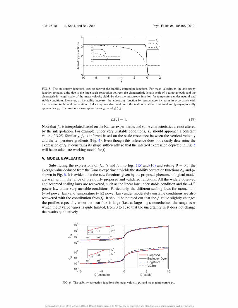
Substituting the expressions of fw, fT and fu into Eqs. (15) and (16) and setting β = 0.5, theaverage value deduced from the Kansas experiment yields the stability correction functions φm and φh

shown in Fig. 6. It is evident that the new functions given by the proposed phenomenological modelare well within the range of previously proposed and validated functions. All the widely observedand accepted scaling laws are recovered, such as the linear law under stable condition and the –1/3power law under very unstable conditions. Particularly, the different scaling laws for momentum(–1/4 power law) and temperature (–1/2 power law) under moderately unstable conditions are alsorecovered with the contribution from fT. It should be pointed out that the β value slightly changesthe profiles especially when the heat flux is large (i.e., at large −ς ); nonetheless, the range overwhich the β value varies is quite limited, from 0 to 1, so that the uncertainty in β does not changethe results qualitatively.

10−1

100

101

102

φ m

10−2

100

102

10−1

100

−1/4−1/3

−10 −510

−2

10−1

100

101

ζ (unstable)

φ h

10−2

100

102

10−1

100

−1/2−1/3

0 5 10ζ (stable)

ProposedBusinger−DyerHogstromVDZ95

FIG. 6. The stability correction functions for mean velocity φm and mean temperature φh.

Downloaded 16 Oct 2012 to 152.3.110.48. Redistribution subject to AIP license or copyright; see http://pof.aip.org/about/rights_and_permissions

105105-11 Li, Katul, and Bou-Zeid Phys. Fluids 24, 105105 (2012)

−10 −5 00

1

2

Pr

ζ (unstable)

ProposedBusinger−Dyer

5 10ζ (stable)

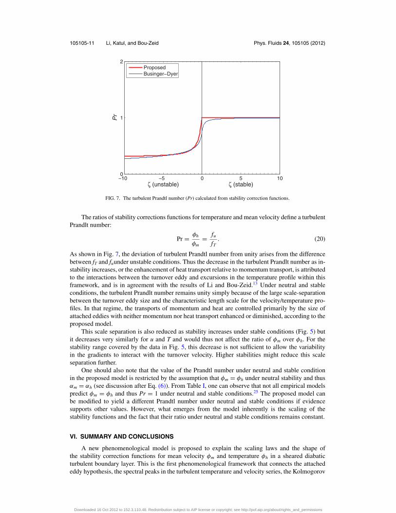
FIG. 7. The turbulent Prandtl number (Pr) calculated from stability correction functions.

The ratios of stability corrections functions for temperature and mean velocity define a turbulentPrandlt number:

Pr = φh

φm= fu

fT. (20)

As shown in Fig. 7, the deviation of turbulent Prandtl number from unity arises from the differencebetween fT and fuunder unstable conditions. Thus the decrease in the turbulent Prandlt number as in-stability increases, or the enhancement of heat transport relative to momentum transport, is attributedto the interactions between the turnover eddy and excursions in the temperature profile within thisframework, and is in agreement with the results of Li and Bou-Zeid.13 Under neutral and stableconditions, the turbulent Prandlt number remains unity simply because of the large scale-separationbetween the turnover eddy size and the characteristic length scale for the velocity/temperature pro-files. In that regime, the transports of momentum and heat are controlled primarily by the size ofattached eddies with neither momentum nor heat transport enhanced or diminished, according to theproposed model.

This scale separation is also reduced as stability increases under stable conditions (Fig. 5) butit decreases very similarly for u and T and would thus not affect the ratio of φm over φh. For thestability range covered by the data in Fig. 5, this decrease is not sufficient to allow the variabilityin the gradients to interact with the turnover velocity. Higher stabilities might reduce this scaleseparation further.

One should also note that the value of the Prandtl number under neutral and stable conditionin the proposed model is restricted by the assumption that φm = φh under neutral stability and thusαm = αh (see discussion after Eq. (6)). From Table I, one can observe that not all empirical modelspredict φm = φh and thus Pr = 1 under neutral and stable conditions.25 The proposed model canbe modified to yield a different Prandtl number under neutral and stable conditions if evidencesupports other values. However, what emerges from the model inherently is the scaling of thestability functions and the fact that their ratio under neutral and stable conditions remains constant.

VI. SUMMARY AND CONCLUSIONS

A new phenomenological model is proposed to explain the scaling laws and the shape ofthe stability correction functions for mean velocity φm and temperature φh in a sheared diabaticturbulent boundary layer. This is the first phenomenological framework that connects the attachededdy hypothesis, the spectral peaks in the turbulent temperature and velocity series, the Kolmogorov

Downloaded 16 Oct 2012 to 152.3.110.48. Redistribution subject to AIP license or copyright; see http://pof.aip.org/about/rights_and_permissions

105105-12 Li, Katul, and Bou-Zeid Phys. Fluids 24, 105105 (2012)

energy cascade for velocity and temperature within the inertial subrange, and the stability correctionfunctions for heat and momentum in the atmosphere. The aim is to provide a theoretical explanationfor scaling of φm and φh with stability and to explain the dissimilarity between momentum and heattransport under unstable conditions. It is found that a straightforward extension of the original modelin Katul et al.12 to temperature results in absolute similarity between φm and φh (i.e., Reynoldsanalogy), given the similarity in the turnover eddy acting on the mean profiles. Hence, such anextension cannot recover the widely reported different scaling laws for φh (–1/2 power law) whencompared to φm (–1/4 power law) in the unstable regime. The failure of this original model, whenextended to temperature, is traced to the interaction between the turnover eddy and excursions in theinstantaneous temperature profiles. This interaction results in dispersive fluxes that augment heatflux, but do not affect momentum flux. Starting from the momentum and sensible heat flux budgets,it is further demonstrated that the dynamic role of temperature variances modulates the length scalecharacterizing the variability in the instantaneous temperature profile and thus enables the scaleresonance causing the dispersive fluxes. These findings then provide the basis for a refinement to theoriginal phenomenological model. This refinement is introduced via a new adjustment to the attachededdy size (i.e., resembling an anisotropy ratio) representing the effect of interactions between theturnover eddy and the excursions in the temperature vertical profiles.

Ignoring these adjustments in the momentum transport is justified by the fact that the integrallength scale of the longitudinal velocity is at least one order of magnitude larger than the size ofthe turnover eddy. However, this is demonstrated not to be the case for temperature under unstableconditions. The integral length scale of the temperature profile, which is approximated by the integrallength scale of the temperature time-series measured at a given point, becomes comparable to theintegral length scale of the turnover velocity. The immediate implications then are that the meantemperature difference at the two end-points of the turnover eddy is no longer a viable indicatorof the size of excursions in the temperature profile across the turnover eddy; but rather, a newlength scale characterizing the size of these excursions has to be introduced. The scale-resonanceor interactions between the turnover eddy and the excursions in the temperature profiles enhancethe heat transport and result in dissimilarity between momentum and temperature. It is also thisscale-resonance mechanism that is responsible for the decrease in the turbulent Prandtl numberunder unstable conditions.

With this new length scale incorporated into the phenomenological model, the stability depen-dence of the generalized model is now guided by the ratio of integral length scales and successfullyrecovers the –1/2 power law scaling law for φh, as well as the dissimilarity between momentum andtemperature under unstable conditions. Under neutral and stable conditions, φh remains the same as,or proportional to φm.

ACKNOWLEDGMENTS

This work is supported by National Science Foundation (NSF) under CBET-1058027 and AGS-1026636. G. G. Katul acknowledges support from NSF through Grant Nos. NSF-EAR-1013339,NSF-AGS-1102227, and NSF-CBET-103347, the United States Department of Agriculture (2011-67003-30222), and the U.S. Department of Energy (DOE) through the office of Biological andEnvironmental Research (BER) Terrestrial Ecosystem Science (TES) Program (DE-SC0006967).The authors would like to thank Professor Marc Parlange, Dr. Hendrik Huwald, Dr. Chad Higgins,and the rest of the team of the Environmental Fluid Mechanics and Hydrology Laboratory at theSwiss Federal Institute of Technology—Lausanne for the collection of the lake and glacier datasetsdescribed here. The authors also thank Professor Jordi Vila-Guerau de Arellano for providing themthe model results in VDZ95.

APPENDIX A: DYNAMIC ROLE OF TEMPERATURE VARIANCES IN INDUCINGDISSIMILARITY BETWEEN MOMENTUM AND HEAT TRANSPORT

The momentum and sensible heat flux budgets are considered for the idealized micromete-orological conditions previously assumed. These budgets are intended to illustrate the causes of

Downloaded 16 Oct 2012 to 152.3.110.48. Redistribution subject to AIP license or copyright; see http://pof.aip.org/about/rights_and_permissions

105105-13 Li, Katul, and Bou-Zeid Phys. Fluids 24, 105105 (2012)

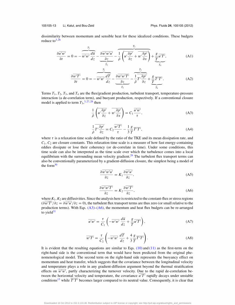
dissimilarity between momentum and sensible heat for these idealized conditions. These budgetsreduce to3, 26

∂u′w′

∂t= 0 = −

T1︷ ︸︸ ︷w′w′ du

dz− ∂w′w′u′

∂z︸ ︷︷ ︸T2

−

T3︷ ︸︸ ︷1

ρ

(u′ ∂p′

∂z+ w′ ∂p′

∂x

)+ g

Tu′T ′︸ ︷︷ ︸T4

, (A1)

∂w′T ′

∂t= 0 = −

T1︷ ︸︸ ︷w′w′ dT

dz− ∂w′w′T ′

∂z︸ ︷︷ ︸T2

−

T3︷ ︸︸ ︷1

ρT ′ ∂p′

∂z+ g

TT ′T ′︸ ︷︷ ︸T4

. (A2)

Terms T1, T2, T3, and T4 are the flux/gradient production, turbulent transport, temperature-pressureinteraction (a de-correlation term), and buoyant production, respectively. If a conventional closuremodel is applied to term T3,3, 27, 28 then

1

ρ

(u′ ∂p′

∂z+ w′ ∂p′

∂x

)= C1

u′w′

τ, (A3)

1

ρT ′ ∂p′

∂z= C2

w′T ′

τ− 1

3

g

TT ′T ′, (A4)

where τ is a relaxation time scale defined by the ratio of the TKE and its mean dissipation rate, andC1, C2 are closure constants. This relaxation time scale is a measure of how fast energy-containingeddies dissipate or lose their coherency (or de-correlate in time). Under some conditions, thistime scale can also be interpreted as the time scale over which the turbulence comes into a localequilibrium with the surrounding mean velocity gradient.29 The turbulent flux transport terms canalso be conventionally parameterized by a gradient-diffusion closure, the simplest being a model ofthe form30

∂w′w′u′

∂z= K1

∂w′u′

∂z, (A5)

∂w′w′T ′

∂z= K2

∂w′T ′

∂z, (A6)

where K1, K2 are diffusivities. Since the analysis here is restricted to the constant-flux or stress regions(∂w′T ′/∂z = ∂w′u′/∂z = 0), the turbulent flux transport terms are thus zero (or small relative to theproduction terms). With Eqs. (A3)–(A6), the momentum and heat flux budgets can be re-arrangedto yield31

u′w′ = τ

C1

(−w′w′ du

dz+ g

Tu′T ′

), (A7)

w′T ′ = τ

C2

(−w′w′ dT

dz+ 4

3

g

TT ′T ′

). (A8)

It is evident that the resulting equations are similar to Eqs. (10) and (11) as the first-term on theright-hand side is the conventional term that would have been predicted from the original phe-nomenological model. The second term on the right-hand side represents the buoyancy effect onmomentum and heat transfer, which suggests that the covariance between the longitudinal velocityand temperature plays a role in any gradient-diffusion argument beyond the thermal stratificationeffects on w′w′, partly characterizing the turnover velocity. Due to the rapid de-correlation be-tween the horizontal velocity and temperature, the covariance u′T ′ rapidly decays under unstableconditions13 while T ′T ′ becomes larger compared to its neutral value. Consequently, it is clear that

Downloaded 16 Oct 2012 to 152.3.110.48. Redistribution subject to AIP license or copyright; see http://pof.aip.org/about/rights_and_permissions

105105-14 Li, Katul, and Bou-Zeid Phys. Fluids 24, 105105 (2012)

a major modification to the earlier phenomenological model must include, at minimum, the effectof the temperature variance on heat transfer. It can be also argued that within the inertial subrange(as we assumed here), u′T ′ decays as k−7/3 while T ′T ′ decays as k−5/3, clearly indicating that therole of buoyancy is more important for heat than for momentum.21

With regards to framing this modification via an effective adjustment to the attached eddy size(= z), note that upon combining σ 2

T /T 2∗ = ϕT T (ς ), the Monin-Obukhov variance-flux similarity

relation with T∗ = dT

dz

κvz

φh (ς )results in σT =

(dT

dz

)z

(κv

√ϕT T (ς )

φh(ς )

). Substituting this expression

into Eq. (A8) gives

w′T ′ = τ

C2

(−σ 2

w

dT

dz+ 4

3

g

TσT

dT

dzz

(κv

√ϕT T (ς )

φh(ς )

))

= −σw

dT

dz

σwτ

C2

⎛⎜⎜⎜⎝1+43

g

TσT z

(κv

√ϕT T (ς )

φh(ς )

)−σw

σwτ

C2

⎞⎟⎟⎟⎠∼ −v (s)

dT

dzs fT (ς ) . (A9)

In Eq. (A9), fT(ς ) can be seen as a “correction” of the length scale (s) due to the effect of thetemperature variance. This is consistent with our analyses that the potential scale-resonance betweenthe turnover eddy and the excursions in the temperature profile (Fig. 5) requires a new length scaleintroduced to the model when extending it to temperature, as shown in Eq. (14).

APPENDIX B: A NEW THEORETICAL DERIVATION FOR AN O’KEYPS EQUATIONFOR TEMPERATURE

In this appendix, it is demonstrated that an O’KEYPS equation describing the heat stabil-ity correction function can be derived from inertial subrange scaling provided the mean tem-perature difference across a turnover eddy linearly scales with the macro-scale properties ofthe eddy. This derivation commences with the phenomenological model for sensible heat flux,

w′T ′ = −αhv (s)[T (z + s) − T (z − s)

]and v (s) = w (s)2

1/2. Postulating that the mean temper-

ature difference across a turnover eddy is now entirely described by the macro-scale propertiesof the eddy, which are due to the large and often coherent ramp-like structures simultaneouslycontributing to the mean temperature gradient and macro-scale temperature difference, implies

that[T (z + s) − T (z − s)

] ∼ (T ′ (z + s) − T ′ (z − s))21/2 ∼ (T (s))2

1/2. For notational simplic-

ity, denote |ψ (s)| = (ψ ′ (x + s) − ψ ′ (x − s))2 for any arbitrary flow variable ψ .From the Kolmogorov theory for the velocity spectrum and the Kolmogorov-Corrsin theory

for the temperature spectrum,32 |w (s)| = Coε1/3s1/3, and |T (s)| = CT χ

1/2T ε−1/6s1/3, where Co

and CT are related to the Kolmogorov constant. Here, χT is the dissipation rate for the temperaturevariance. Hence, at s = z and with w′T ′ = −T∗u∗, the sensible heat flux is now given as

αhCT Coχ1/2T ε1/6z2/3

T∗u∗= 1. (B1)

As per Eq. (7), ε = u3∗

kv z (φm (ς ) − ς ), and by invoking the local equilibrium assumption stating thatthe dissipation rate is equal to the production rate for the mean temperature variance,33 namely,

χT = −w′T ′ dT

dz= u∗

T 2∗

κvzφh (ς ), we obtain

αhCT Co

(u∗

T 2∗

κv z φh (ς ))1/2 ( u3

∗κv z (φm (ς ) − ς )

)1/6z2/3

T∗u∗= 1. (B2)

Downloaded 16 Oct 2012 to 152.3.110.48. Redistribution subject to AIP license or copyright; see http://pof.aip.org/about/rights_and_permissions

105105-15 Li, Katul, and Bou-Zeid Phys. Fluids 24, 105105 (2012)

Simplifying this expression further leads to(αhCT Co

κ2/3v

)φh (ς )1/2 (φm (ς ) − ς)1/6 = 1. (B3)

Again, upon imposing φh(0) = φm(0) = 1 for ς = 0, Eq. (B3) yields

[φh (ς )]3 φm (ς )

(1 − ς

φm (ς )

)= 1. (B4)

It is evident that this formula is identical to Eq. (9), which was a straightforward extension of theoriginal phenomenological model. When φh(ς ) = φm(ς ), it also recovers the canonical form of theO’KEYPS equation,12 or Eq. (8).

Furthermore, deviations from the canonical energy cascade and temperature variance cascadecan be readily accounted for via intermittency corrections (s/Iw)μ1 and (s/IT )μ2 , respectively, whereIw and IT are the integral length scales for vertical velocity and temperature, and μ1 and μ2 are theintermittency correction coefficients.34, 35

These intermittency corrections result in |w (s)| = Coε1/3s1/3(s/Iw)μ1 and |T (s)|

= CT χ1/2T ε−1/6s1/3(s/IT )μ2 . Similar to previous derivations, the final outcome with these inter-

mittency corrections is

[φh (ς )]3 φm (ς )

(1 − ς

φm (ς )

)= 1

g6μ1w g6μ2

T

, (B5)

where gw = z

Iwand gT = z

IT. Note that gw and gT vary with the integral length scales Iw and IT, as

previously demonstrated in Eq. (16). In addition, as discussed in Warhaft,24 ramp-cliff structures inthe temperature field result in μ1 ≤μ2,which appears to be qualitatively consistent with Eq. (16) giventhat the differences here between φh and φm also originate from variations in the temperature gradientscale caused by ramps (i.e., large-scale impacting inertial subrange) on intermittency parameters.

1 W. Brutsaert, Hydrology: An Introduction (Cambridge University Press, New York, 2005).2 A. S. Monin and A. M. Obukhov, “Basic laws of turbulent mixing in the ground layer of the atmosphere,” Akad. Nauk.

SSSR, Geofiz. Inst. Trudy 151, 163 (1954).3 R. B. Stull, An Introduction to Boundary Layer Meteorology (Kluwer Academic, Dordrecht, 1988).4 W. Brutsaert, Evaporation into the Atmosphere: Theory, History, and Applications (Reidel, Dordrecht, 1982), Environmental

fluid mechanics.5 J. A. Businger, “A note on the Businger-Dyer profiles,” Boundary-Layer Meteorol. 42, 145 (1988).6 J. Vila-Guerau de Arellano, P. G. Duynkerke, and K. F. Zeller, “Atmospheric surface-layer similarity theory applied to

chemically reactive species,” J. Geophys. Res., [Atmos.] 100, 1397, doi:10.1029/94JD02434 (1995).7 S. Khanna and J. G. Brasseur, “Analysis of Monin-Obukhov similarity from large-eddy simulation,” J. Fluid Mech. 345,

251 (1997).8 U. Hogstrom, “Non-dimensional wind and temperature profiles in the atmospheric surface-layer - A re-evaluation,”

Boundary-Layer Meteorol. 42, 55 (1988).9 D. K. Wilson, “An alternative function for the wind and temperature gradients in unstable surface layers - Research note,”

Boundary-Layer Meteorol. 99, 151 (2001).10 B. A. Kader and A. M. Yaglom, “Mean fields and fluctuation moments in unstably stratified turbulent boundary-layers,” J.

Fluid Mech. 212, 637 (1990).11 G. Gioia et al., “Spectral theory of the turbulent mean-velocity profile,” Phys. Rev. Lett. 105, 184501 (2010).12 G. G. Katul, A. G. Konings, and A. Porporato, “Mean velocity profile in a sheared and thermally stratified atmospheric

boundary layer,” Phys. Rev. Lett. 107, 268502 (2011).13 D. Li and E. Bou-Zeid, “Coherent structures and the dissimilarity of turbulent transport of momentum and scalars in the

unstable atmospheric surface layer,” Boundary-Layer Meteorol. 140, 243 (2011).14 E. Bou-Zeid et al., “Field study of the dynamics and modelling of subgrid-scale turbulence in a stable atmospheric surface

layer over a glacier,” J. Fluid Mech. 665, 480 (2010).15 A. A. Townsend, The Structure of Turbulent Shear Flow, 2nd ed. (Cambridge University Press, Cambridge, England,

1976), Cambridge monographs on mechanics and applied mathematics.16 A. J. Smits, B. J. McKeon, and I. Marusic, “High-Reynolds number wall turbulence,” Annu. Rev. Fluid Mech. 43, 353

(2011).17 J. A. Businger and A. M. Yaglom, “Introduction to Obukhov’s paper on ‘turbulence in an atmosphere with a non-uniform

temperature’,” Boundary-Layer Meteorol. 2, 3 (1971).18 N. Vercauteren et al., “Subgrid-scale dynamics of water vapour, heat, and momentum over a lake,” Boundary-Layer

Meteorol. 128, 205 (2008).

Downloaded 16 Oct 2012 to 152.3.110.48. Redistribution subject to AIP license or copyright; see http://pof.aip.org/about/rights_and_permissions

105105-16 Li, Katul, and Bou-Zeid Phys. Fluids 24, 105105 (2012)

19 E. Bou-Zeid et al., “Scale dependence of subgrid-scale model coefficients: An a priori study,” Phys. Fluids 20, 115106(2008).

20 D. Li, E. Bou-Zeid, and H. De Bruin, “Monin–Obukhov similarity functions for the structure parameters of temperatureand humidity,” Boundary-Layer Meteorol. 145(1), 45–67 (2012).

21 J. C. Kaimal and J. J. Finnigan, Atmospheric Boundary Layer Flows: Their Structure and Measurement (Oxford UniversityPress, New York, 1994).

22 A. Kolmogoroff, “The local structure of turbulence in incompressible viscous fluid for very large Reynolds numbers,” C.R. Acad. Sci. URSS 30, 301 (1941).

23 S. Corrsin, “On the spectrum of isotropic temperature fluctuations in an isotropic turbulence,” J. Appl. Phys. 22, 469(1951).

24 Z. Warhaft, “Passive scalars in turbulent flows,” Annu. Rev. Fluid Mech. 32, 203 (2000).25 W. M. Kays, “Turbulent Prandtl number - Where are we,” J. Heat Transfer 116, 284 (1994).26 M. Siqueira and G. Katul, “Estimating heat sources and fluxes in thermally stratified canopy flows using higher-order

closure models,” Boundary-Layer Meteorol. 103, 125 (2002).27 T. Meyers and K. T. P. U, “Testing of a higher-order closure-model for modeling air-flow within and above plant canopies,”

Boundary-Layer Meteorol. 37, 297 (1986).28 C. H. Moeng and J. C. Wyngaard, “An analysis of closures for pressure-scalar covariances in the convective boundary-

layer,” J. Atmos. Sci. 43, 2499 (1986).29 S. E. Belcher and J. C. R. Hunt, “Turbulent flow over hills and waves,” Annu. Rev. Fluid Mech. 30, 507 (1998).30 G. G. Katul, A. M. Sempreviva, and D. Cava, “The temperature-humidity covariance in the marine surface layer: A

one-dimensional analytical model,” Boundary-Layer Meteorol. 126, 263 (2008).31 D. Cava et al., “Buoyancy and the sensible heat flux budget within dense canopies,” Boundary-Layer Meteorol. 118, 217

(2006).32 A. S. Monin and A. M. Yaglom, Statistical Fluid Mechanics (MIT, Cambridge, MA, 1975).33 C. I. Hsieh and G. G. Katul, “Dissipation methods, Taylor’s hypothesis, and stability correction functions in the atmospheric

surface layer,” J. Geophys. Res., [Atmos.] 102, 16391, doi:10.1029/97JD00200 (1997).34 A. N. Kolmogorov, “A refinement of previous hypotheses concerning the local structure of turbulence in a viscous

incompressible fluid at high Reynolds number,” J. Fluid Mech. 13, 82 (1962).35 U. Frisch, Turbulence: The Legacy of A.N. Kolmogorov (Cambridge University Press, Cambridge, England, 1995).

Downloaded 16 Oct 2012 to 152.3.110.48. Redistribution subject to AIP license or copyright; see http://pof.aip.org/about/rights_and_permissions