Diabatic processes and the evolution of two contrasting summer extratropical cyclones Article

Accepted Version

Martinez­Alvarado, O., Gray, S. L. and Methven, J. (2016) Diabatic processes and the evolution of two contrasting summer extratropical cyclones. Monthly Weather Review, 144 (9). pp. 3251­3276. ISSN 0027­0644 doi: https://doi.org/10.1175/MWR­D­15­0395.1 Available at http://centaur.reading.ac.uk/65848/

It is advisable to refer to the publisher’s version if you intend to cite from the work. See Guidance on citing .

To link to this article DOI: http://dx.doi.org/10.1175/MWR­D­15­0395.1

Publisher: American Meteorological Society

All outputs in CentAUR are protected by Intellectual Property Rights law, including copyright law. Copyright and IPR is retained by the creators or other copyright holders. Terms and conditions for use of this material are defined in the End User Agreement .

www.reading.ac.uk/centaur

CentAUR

Central Archive at the University of Reading

Reading’s research outputs online

Diabatic processes and the evolution of two contrasting

summer extratropical cyclones

Oscar Martınez-Alvarado1,2, Suzanne L. Gray2 and John Methven2

1 National Centre for Atmospheric Science–Atmospheric Physics, United Kingdom2 Department of Meteorology, University of Reading, United Kingdom

June 14, 2016

Correspondence to:Oscar Martınez-AlvaradoDepartment of Meteorology, University of ReadingEarley Gate, Reading, RG6 6BB, United KingdomE-mail: o.martinezalvarado@reading.ac.ukTel: +44 (0) 118 378 8951Fax: +44 (0) 118 378 8905

1

Abstract

Extratropical cyclones are typically weaker and less frequent in summer as a result of dif-

ferences in the background state flow and diabatic processes with respect to other seasons.

Two extratropical cyclones were observed in summer 2012 with a research aircraft during

the DIAMET (DIAbatic influences on Mesoscale structure in ExTratropical storms) field

campaign. The first cyclone deepened only down to 995 hPa; the second cyclone deepened

down to 978 hPa and formed a potential vorticity (PV) tower, a frequent signature of intense

cyclones. The objectives of this article are to quantify the effects of diabatic processes and

their parametrizations on cyclone dynamics. The cyclones were analyzed through numerical

simulations incorporating tracers for the effects of diabatic processes on potential tempera-

ture and PV. The simulations were compared with radar rainfall observations and dropsonde

measurements. It was found that the observed maximum vapor flux in the stronger cyclone

was twice as strong as in the weaker cyclone; the water vapor mass flow along the warm

conveyor belt of the stronger cyclone was over half that typical in winter. The model over-

estimated water vapor mass flow by approximately a factor of two due to deeper structure

in the rearwards flow and humidity in the weaker case. An integral tracer interpretation is

introduced, relating the tracers with cross-isentropic mass transport and circulation. It is

shown that the circulation around the cyclone increases much more slowly than the amplitude

of the diabatically-generated PV tower. This effect is explained using the PV impermeability

theorem.

1 Introduction

Intense precipitation in summer over western Europe is largely associated with the passage

of extratropical cyclones. Using data from the Global Precipitation Climatology Product

daily precipitation dataset (Huffman et al., 2001; Adler et al., 2003) and the ECMWF ERA-

Interim reanalysis product (Simmons et al., 2007; Dee et al., 2011), Hawcroft et al. (2012)

determined that more than 65% of total precipitation during June–July–August is associated

with extratropical cyclones over the United Kingdom, Northern Europe and Scandinavia.

Heavy precipitation can have an important societal impact as it can lead to extreme weather

events such as flash flooding. Water vapor condensation in the rising air also releases latent

heat, which typically intensifies the ascending motion and the cyclone near the surface (e.g.

Tracton, 1973; Davis, 1992; Stoelinga, 1996; Ahmadi-Givi et al., 2004; Grams et al., 2011).

For example, studying a cyclone that reached its maximum intensity (based on mean sea

level pressure) on 24 February 1987, Stoelinga (1996) showed that its intensity was 70%

stronger as a result of coupling between baroclinic wave growth and latent heat release.

Until now, studies on latent heat release and cyclone intensification have focused on Northern

Hemisphere extratropical cyclones occurring mostly during winter time (December–January–

February), but also during spring (March–April–May) and autumn (September–October–

November). On the other hand, the importance of latent heat release, and diabatic processes

2

in general, for the development of summer extratropical cyclones has received much less

attention.

Summer extratropical cyclones are generally less frequent and weaker than their winter

counterparts. In an analysis of the ERA-Interim dataset between 1989 and 2009, Campa and Wernli

(2012) showed that the central mean sea level pressure of winter cyclones in the Northern

Hemisphere can be found in the range between 930 hPa and 1030 hPa, with around 45%

occurring in the band between 990 hPa and 1010 hPa and 15% occurring in the lowest band

between 930 hPa and 970 hPa. In contrast, Northern Hemisphere summer cyclones can be

found within the same range, but 83% occur in the band between 990 hPa and 1010 hPa and

only 0.2% in the lowest band between 930 hPa and 970 hPa. These differences are arguably

due to differences in the environmental conditions between summer and winter. The envi-

ronmental differences include different background state flows as well as higher temperature

and saturation humidity, reduced ice phase and increased insolation during summer. Despite

these differences it can be hypothesized that diabatic processes contribute to the intensifica-

tion of summer cyclones as much as they contribute to the intensification of cyclones in winter

and other seasons. Indeed, Dearden et al. (2016) showed that ice processes, such as depo-

sitional growth, sublimation and melting, are important in determining a summer cyclone’s

minimum central pressure and track. However, more work is needed to fully understand the

importance of diabatic processes in general for cyclone intensification in summer.

This article has two objectives. The first objective is to quantify the heating (calculated as

the change in potential temperature following an air parcel) produced during the occurrence

of two contrasting summer extratropical cyclones and assess the effects of this heating in

terms of changes to the circulation around the cyclones. In contrast to Dearden et al. (2016),

the analysis is not restricted to ice processes. Instead, all the diabatic processes represented

in the model by parametrization schemes are included. The second objective is to determine

the contribution that each relevant parametrization scheme made to the total heating and

its effects in these two cyclones. These objectives are pursued through simulations with a

numerical model that requires the parametrization of convection. The model includes tracers

of diabatic effects on potential temperature (e.g. Martınez-Alvarado and Plant, 2014) and

potential vorticity (PV) (e.g. Stoelinga, 1996; Gray, 2006).

The two cyclones occurred during the last field campaign of the DIAMET (DIAbatic

influences on Mesoscale structures in ExTratropical storms) project (Vaughan et al., 2015),

which took place in the summer of 2012. Dearden et al. (2016) use the same two cases to

examine the effect of ice phase microphysical processes on summer extratropical cyclones

dynamics. Both cyclones developed bent-back fronts and exhibited prolonged periods of

heavy frontal precipitation (Fig. 1(a,b)). Despite these similarities, the two cyclones represent

two very different intensity scenarios for summer. The first cyclone reached a central pressure

minimum of 995 hPa on 19 July 2012. Its central pressure places it in the most frequent

cyclone category for summer cyclones over western Europe (Campa and Wernli, 2012): five

out of an average of seven annual summer cyclones that reach maximum intensity over western

3

Table 1: Number of cyclones over western Europe in summer (June–July–August) and win-ter (December–January–February) in the ERA-Interim dataset for the period between 1989and 2009. The definition of western Europe and the frequency columns were taken fromCampa and Wernli (2012).

Summer WinterNumber Occurrence Number Occurrence

of cyclones per year of cyclones per year930–970 hPa 1 0.05 33 1.65970–990 hPa 16 0.80 64 3.20990–1010 hPa 99 4.95 75 3.751010–1030 hPa 15 0.75 10 0.50

Total 131 6.55 182 9.10

Europe have a minimum sea level pressure between 990 hPa and 1010 hPa (Table 1). In

contrast, the second cyclone reached a central pressure minimum of 978 hPa on 15 August

2012. Only 0.8 summer cyclones per year on average have a minimum sea level pressure

between 970 hPa and 990 hPa (Table 1). Given its minimum sea level pressure, this cyclone

would be more typical of winter than summer.

The rest of the article is organized as follows. The available aircraft observations, nu-

merical model and diabatic tracers are described in Section 2; Section 3 is devoted to the

comparison of the simulations with the available observations; the results are presented and

discussed in Sections 4 and 5, which deal with the July and August cases, respectively, and in

Section 6, which makes a comparison in terms of diabatic processes between the two cyclones;

conclusions are given in Section 7.

2 Data and methods

2.1 Available aircraft observations

The cyclone on 18 July 2012 was the subject of the DIAMET Intensive Observation Period

(IOP) 13 while the cyclone on 15 August 2012 was the subject of the DIAMET IOP14. Both

cyclones were observed with the instruments on board the Facility for Airborne Atmospheric

Measurements (FAAM) BAe146 research aircraft (Vaughan, 2011). See Vaughan et al. (2015)

for a summary of the instruments, their sampling frequency and uncertainty on output pa-

rameters.

The dropsonde system is essentially the same as that described by Martınez-Alvarado et al.

(2014b). In the flights discussed in this work, the average sonde spacing was limited to a

minimum of 4 minutes along the flight track or 24 km at the aircraft science speed, i.e. the

aircraft speed that ensures consistent instrument performance, of 100 m s−1. Eight dropson-

des were released at regular time intervals during both flights, between 0830 UTC and 0902

UTC 18 July 2012 during IOP13 and between 1534 UTC and 1603 UTC 15 August 2012

during IOP14.

4

2.2 Hindcast simulations

The simulations have been performed using the MetUM version 7.3 which is based on

the so-called “New Dynamics” dynamical core (Davies et al., 2005). The model configu-

ration, vertical and horizontal resolutions and the domain used here are the same as in

Martınez-Alvarado et al. (2014b). The model description follows Martınez-Alvarado et al.

(2014b) with minor modifications to accommodate details relevant to this work. The simula-

tions have been performed on a limited-area domain corresponding to the Met Office’s recently

operational North-Atlantic–European domain with 600×300 grid points. The horizontal grid

spacing is 0.11 (∼ 12 km) in both longitude and latitude on a rotated grid centered around

52.5N, 2.5W. The North-Atlantic–European domain extends approximately from 30N to

70N in latitude and from 60W to 40E in longitude. The vertical coordinate is discretized

in 70 vertical levels with lid around 80 km. The initial conditions were given by Met Office

operational analyses valid at 1200 UTC 17 July 2012, for IOP13, and at 1800 UTC 14 Au-

gust 2012, for IOP14. The lateral boundary conditions (LBCs) consisted of the Met Office

operational 3-hourly LBCs valid from 0900 UTC 17 July 2012 for 72 hours, for IOP13, and

from 1500 UTC 14 August 2012 for 72 hours, for IOP14.

2.3 Diabatic tracers

The MetUM has been enhanced by the inclusion of diabatic tracers of potential temperature

(θ) and PV (Martınez-Alvarado et al., 2015). The description of diabatic tracers in this

section is derived from Martınez-Alvarado and Plant (2014) and Martınez-Alvarado et al.

(2015) with updates and additional details relevant to this work.

Diabatic tracers of θ and PV track θ and PV changes due to diabatic processes. Dia-

batic potential temperature tracers enable identification of the processes (including turbu-

lent mixing and resolved advection) that bring air parcels to their current isentropic level

through cross-isentropic motion. Cross-isentropic motion is interpreted as vertical motion

in isentropic coordinates so that a positive change in θ indicates mean cross-isentropic as-

cent while a negative change in θ indicates mean cross-isentropic descent. Notice that

cross-isentropic ascent does not imply an increase in height, as an air parcel can experi-

ence an increase in θ while conserving its geopotential height. Similarly, an increase in

height does not imply cross-isentropic ascent as an air parcel can ascend adiabatically. Di-

abatic PV tracers enable identification of modifications to the circulation and stability and

the diabatic processes responsible for such modifications. Diabatic θ tracers have been

previously described in Martınez-Alvarado and Plant (2014) and Martınez-Alvarado et al.

(2014b), while the diabatic PV tracer technique has been developed by in Stoelinga (1996),

Gray (2006), Chagnon and Gray (2009), Chagnon et al. (2013), Chagnon and Gray (2015)

and Saffin et al. (2015). The diabatic tracers described here are conceptually related to those

described by Cavallo and Hakim (2009) and Joos and Wernli (2012). However, those meth-

ods analyse Lagrangian tendencies whereas diabatic tracers can be interpreted as time inte-

5

grals of diabatic tendencies along trajectories. Diabatic tracers of θ and PV have been used to-

gether in the analysis of forecast errors in upper-level Rossby waves (Martınez-Alvarado et al.,

2015).

The idea behind diabatic tracers of θ and PV consists of the separation of the variable of

interest ϕ (representing either θ or PV) into the sum of a materially-conserved component,

ϕ0, a diabatically-generated component, ϕd, and a residual, rϕ, i.e.

ϕ(x, t) = ϕ0(x, t) + ϕd(x, t) + rϕ(x, t), (1)

where x represents spatial location and t is time. The materially-conserved and the diabatically-

generated parts are governed by the following equations

Dϕ0

Dt= 0 (2)

Dϕd

Dt= Sϕ, (3)

where Sϕ represents a source due to diabatic processes,

D

Dt=

∂

∂t+ u · ∇,

and u = (u, v, w) is the three-dimensional velocity field. In other words, ϕ0 is unaffected

by diabatic processes, and therefore conserved following an air parcel, while ϕd is affected

by diabatic processes. Since ϕ0 is only affected by advection, this tracer has also been

called an advection-only tracer in other works (Chagnon et al., 2013; Chagnon and Gray,

2015; Saffin et al., 2015). The sum of (2) and (3) yields the full evolution equation for ϕ,

under the assumption of a small residual. At initialisation time, t0, ϕ0(x, t0) = ϕ(x, t0) and

ϕd(x, t0) = 0. The boundary conditions for ϕ0 are the boundary conditions for ϕ while the

values of ϕd are set to zero in the boundary.

Diabatic tracers can be further extended to the analysis of individual diabatic processes

by separating ϕd into a series of tracers ϕp

ϕd =∑

p∈proc

ϕp, (4)

where proc is the set of parametrized diabatic processes in the model. In this work we

consider contributions from four parametrized processes, namely (i) boundary layer (BL)

and turbulent mixing processes, (ii) convection, (iii) cloud microphysics and (iv) radiation.

The term cloud microphysics is used here to refer to two parametrizations, namely the large-

scale cloud parametrization and the large-scale precipitation parametrization. The latter

includes the following microphysical processes (Wilson and Ballard, 1999): fall of ice from

one layer to the next, homogeneous nucleation of ice from liquid, heterogeneous nucleation of

ice from liquid or vapor, depositional growth/evaporation of ice from liquid or vapor, riming

6

of liquid by ice, capture of raindrops by ice, evaporation of melting ice, melting of ice to

rain, evaporation of rain, accretion of liquid water droplets by rain and autoconversion of

liquid cloud water to rain. The contribution from gravity wave drag to the modification of

PV has also been computed, but is much smaller in comparison with processes (i)–(iv) and

therefore is not shown. Each tracer is selectively affected by the p-th parametrized process

and governed by the equationDϕp

Dt= Sϕ,p, (5)

where Sϕ,p represents the source due to the p-th parametrized process so that

Sϕ =∑

p∈proc

Sϕ,p. (6)

Equations (2), (3) and (5) are solved using the same numerical methods implemented

in the MetUM to solve the evolution equations of the model’s prognostic variables (velocity

components, θ and moisture variables) (cf. Davies et al., 2005). However, there are details

in the numerical representation of the equations of motion which have been specifically de-

signed for the prognostic variables. These details include the staggered distribution of the

variables on the Arakawa C-grid, which imply differences in the advection of PV computed

from prognostic variables and as a tracer (Whitehead et al., 2014), or the treatment of the

advection of θ (Davies et al., 2005). These details lead to an unavoidable mismatch between

the advection of ϕ and that of the sum ϕ0+ϕd in (1). This mismatch gives rise to the residual

term in that equation. The residual grows over time in both cases, but at a slower rate for

the θ tracers than for PV tracers. However, restricting the length of the simulations to less

than 24 hours also restricts the residual growth. For more details regarding the growth of

the residual in PV tracers the reader is referred to Saffin et al. (2015).

2.4 Integral interpretation of θ tracers: Cross-isentropic mass trans-

port

Given that the θ0 tracer is materially-conserved and represents the θ field at the start of

the simulation, it can be used as a Lagrangian label for the vertical position (in isentropic

coordinates) of air masses at the start of the simulation. An integral interpretation of the θ

tracers can be achieved by analyzing the evolution of the θ0 tracer within volumes around the

cyclones’ centers defined by minimum mean sea level pressure. At each considered time, the

grid points within a 1000-km radius cylinder centered at the cyclone’s center were classified

according to their θ0-value into seven 10-K width bins with centers at θ0 = 275 + 10k [K] for

k = 0, 1, . . . , 6. This operation produces a population of grid points for each θ0-bin, which

can then be analyzed separately. The θ0 distributions were computed hourly from the first

hour of each simulation until the end of each simulation (i.e. 21 hours). This methodology is

applied in Section 66.1 to determine the net heating experienced by air in each θ0-bin, and

the contributions from individual diabatic processes to these changes, as a function of time

7

in each cyclone.

2.5 Integral interpretation of PV tracers: Circulation

Ertel PV is defined as (e.g. Haynes and McIntyre, 1987)

Q =1

ρ∇× ua · ∇θ, (7)

where ρ is density, ua = Ω× r + u is the three-dimensional absolute velocity with r being a

position vector from the Earth’s center and Ω being the planetary angular velocity, and ∇

is the gradient operator in geographic coordinates. The absolute circulation on an isentropic

surface is given by

Cθ =

∮

C

ua · dl =

∫

R

∇× ua · kθ dS, (8)

where C is a closed contour on the isentropic surface enclosing region R, dl is a line element

on contour C, dS is a surface element on region R and kθ is a unit vector normal to the

isentropic surface. kθ can be written in terms of ∇θ as

kθ =∇θ

|∇θ|, (9)

while dS is given by

dS =

(

∂θ

∂z

)−1

|∇θ| dx dy, (10)

where dx dy is the projection of area element dS onto the horizontal and z is geopotential

height. This expression is valid as long as θ is a monotonically increasing function of height.

Substituting (9) and (10) into (8) yields

Cθ =

∫

R

(

∂θ

∂z

)−1

∇× ua · ∇θ dx dy. (11)

Using (7) and defining the isentropic density as

σ = ρ

(

∂θ

∂z

)−1

, (12)

we can write

Cθ =

∫

R

σ Qdxdy. (13)

Using (1) PV can be written as

Q = Q0 + Qd + rQ, (14)

where Q0, Qd and rQ are the materially-conserved, the diabatically-generated and the residual

parts of PV, respectively. Multiplying (14) by σ and integrating over the isentropic region R

8

we obtain

Cθ = C0 + Cd + Cr, (15)

where

C0 =

∫

R

σ Q0dx dy and Cd =

∫

R

σ Qddx dy, (16)

i.e. C0 and Cd are contributions to the circulation on isentropic surfaces that can be directly

associated with the materially-conserved and the diabatically-generated parts of PV. The

contribution associated with the residual is assumed small, given that the duration of the

simulations is limited to satisfy this condition, but can be computed as Cr = Cθ − (C0 +Cd).

Dividing (15) by∫

Rdx dy we obtain

ζθ = ζθ,0 + ζθ,d + ζθ,r, (17)

where ζθ is area-averaged isentropic vorticity, ζθ,0 and ζθ,d are the contributions associated

with the materially-conserved and diabatically-generated parts of PV, respectively, and ζθ,r

is the contribution associated with rQ. These results are valid for any isentropic surface.

However, the computations can be carried out for a set of isentropic levels at different time

steps to construct time series of vertical profiles for ζθ, ζθ,0 and ζθ,d, as is done in Section 66.1.

3 Comparison between simulations and observations

The two extratropical cyclones in this study exhibited similarities. The IOP13 cyclone trav-

elled around 600 km during 18 July 2012; the IOP14 cyclone travelled around 700 km during

15 August 2012. Furthermore, both cyclones produced precipitation for prolonged periods.

Precipitation associated with the IOP13 cyclone started around 1800 UTC 17 July 2012 over

Northern Ireland and ended at around 0100 UTC 19 July 2012 across northern England.

Radar rainfall rates at 0900 UTC 18 July 2012 show heavy precipitation on a band over

Scotland, corresponding to the detached warm front, and scattered precipitation over the

south-west of England, corresponding to weak precipitation at the cold front (Fig. 1a). Pre-

cipitation associated with the IOP14 cyclone started before 0000 UTC 15 August 2012 and

continued until the end of the day, passing over the United Kingdom and Ireland from south

to north (Fig. 1b). These features were well represented by the simulations. Figure 1c shows

the rainfall rate for IOP13 derived from the simulation corresponding to the time shown

in Fig. 1a (i.e. T+21). Figure 1d shows the corresponding rainfall rate for IOP14 for the

time shown in Fig. 1b (i.e. T+22). In both cases, the simulations compare well with radar

observations in terms of location and intensity of precipitating features, bar differences in

the resolutions of both datasets. However, one feature that the model fails to represent is

the clear split into two precipitation bands over the east of England in IOP14 due to the

gap between the system’s cold and warm fronts (Fig. 1b) even though the model is able to

represent the gap in the equivalent potential temperature, θe, field.

Despite the similarities in speed and precipitation, the cyclones represent very different

9

synoptic conditions. The synoptic chart for IOP13 at 0600 UTC 19 July 2012 shows a

T-bone structure (Shapiro and Keyser, 1990) (Fig. 1e). The IOP13 cyclone was a shallow

system that deepened slightly after the time shown, reaching 995 hPa at 0600 UTC 19 July

2012. However, its structure remained largely the same from 0600 UTC 18 July 2012 until the

end of its life cycle. In contrast, the IOP14 cyclone was a relatively deep system for a summer

cyclone. Figure 1f shows the IOP14 cyclone at 1200 UTC 15 August 2012 with its bent-back

front (analyzed as an occluded front) wrapped up around the system’s low-pressure center.

These features were also well represented by the simulations as indicated by the 850-hPa θe

isolines, in Figs. 1(c,d) (Notice that there is a three-hour mismatch between Figs. 1(a,c) and

1e and a four-hour mismatch between Figs. 1(b,d) and 1f). Further comparisons between

the simulation and operational Met Office analysis charts were performed in terms of cyclone

position and intensity (central pressure). For IOP13, during the interval between 1800 UTC

17 July 2012 and 1200 UTC 18 July 2012 inclusive, the maximum position error is 151 km

while the maximum error in minimum sea level pressure is 4 hPa. For IOP14, during the

interval between 0000 UTC and 1800 UTC 15 August 2012 inclusive, the maximum position

error is 218 km while the maximum error in minimum sea level pressure is 11 hPa. The cyclone

in IOP14 deepens at a faster rate in the simulation than in analysis at the beginning of the

study period. In spite of this, the simulations can be considered a realistic representation of

the development of both cyclones.

Several quantities derived from the dropsonde observations during the first IOP13 leg are

shown in a vertical cross section in Figs. 2(a,c). Figure 2a shows zonal velocity, u, θ and

relative humidity with respect to ice, RHice; Fig. 2c shows θe and water vapor flux defined as

φq = ρqvH , where q is specific humidity and vH is the horizontal wind component across the

section. Easterly winds of more than 10 m s−1, constituting the system’s cold conveyor belt

(CCB), are confined below 900 hPa. These winds are located around 57.5N within a region

of strong horizontal θe gradient, which corresponds to the system’s warm front (Fig. 2c).

Westerly winds of similar magnitude, located south of the warm front, extend to pressures as

low as 650 hPa. The system’s warm conveyor belt (WCB) is located around 400 hPa. The

CCB and WCB have been identified by their position relative to the cyclone’s center and

surface fronts. A column with RHice > 90% extends from the surface to pressures around 450

hPa. The maximum westward φq is confined below 900 hPa within the warm front region,

between 57N and 58N. Considering only φq with a westward component in Fig. 2c (i.e.

φq < 0) produces a total water vapor mass flow across the vertical dropsonde curtain below

7 km (∼ 400 hPa) of Φq,IOP13 = 1.99 × 107 kg s−1.

Figures 2(b,d) show vertical sections through segment A–B (Fig. 1c) for the same quanti-

ties as in Figs. 2(a,c), but derived from the simulation at 0900 UTC 18 July 2012 (T+21). Seg-

ment A–B approximately corresponds to the aircraft’s track during the first IOP13 dropsonde

leg. Zonal velocity has similar magnitude in model and observations (Fig. 2b). However, the

system’s CCB extends further up in the model than in observations, reaching 850 hPa. The

column with RHice > 90% also extends higher in the model than in observations, indicating

10

that the model’s atmosphere is too moist. This wet bias is a deficiency that has been previ-

ously identified in other studies using the MetUM version 7.3 (e.g Martınez-Alvarado et al.,

2014a). A systematic wet bias in a model could be leading to an overestimation of WCB

intensities and outflow levels as well as tropopause height (Schafler and Harnisch, 2015). Fur-

thermore, Joos and Wernli (2012) showed that evaporation of rain contributes to low-level

PV modification. Therefore, the evaporation in unsaturated air and hence the low-level dia-

batic PV modification might be underestimated by a model exhibiting a wet bias; however,

it is not possible to quantify these effects with the available observations. The position of

the warm front is similar in model and observations (Fig. 2d). The gradient of θe appears

stronger in the model, especially below 800 hPa. However, this apparent difference is due to

the spacing of dropsondes. Analysis of in-situ observations during a transect flight through

the front suggests that the front width was approximately 25 km with a velocity step at the

lowest flight level (∼ 957 hPa) of 12 m s−1 (i.e. an horizontal shear of 5 × 10−4 s−1). The

vertical structure of φq is also similar in model and observations. The maximum φq with a

westward component is located within the region of maximum θe gradient and confined be-

low 900 hPa (Fig. 2d). However, its magnitude is around 50% stronger in the model than in

observations, as a result of stronger u and higher moisture in the model than in observations.

Thus, Φq,IOP13,sim = 4.40 × 107 kg s−1 according to the model, i.e. more than twice as much

as in the observations.

Now we compare the dropsonde observations obtained during IOP14 with the simulation

at 1600 UTC 15 July 2012 (T+22). The vertical structure of dropsonde-derived u, θ and

RHice is shown in Fig. 3a while that of φq and θe is shown in Fig. 3c. In this case, the

flow moves westwards across the whole dropsonde curtain (Fig. 3a). The maximum zonal

velocity (|u| > 30 m s−1) is located at mid-tropospheric levels around 450 hPa, constituting

the system’s WCB. At lower levels, the maximum zonal velocity (|u| > 20 m s−1) is located

within a low-level jet (LLJ) towards the section’s northern edge behind the system’s cold front.

The cold front is located around 55.5N near the surface. A column with RHice > 90% extends

over the cold front to the upper part of the vertical section (Fig. 3a). In this case, φq exhibits

maximum intensity (|φq| > 0.25 kg m−2 s−1) towards the section’s northern edge (Fig. 3c).

This flux produces a water vapor mass flow with a westward component across the vertical

curtain below 7 km of Φq,IOP14 = 1.17 × 108 kg s−1. This value is comparable in magnitude

to the typical meridional water vapor mass flow in a Northern Hemisphere atmospheric river

Φq,AR = 2.2 × 108 kg s−1 (Zhu and Newell, 1998). Figure 3 also shows vertical sections for

model-derived variables through segment C–D (Fig. 1d), which corresponds to the aircraft’s

track during the IOP14 dropsonde leg. In the model, the LLJ core (|u| > 25 m s−1) appears in

the section around 55.5N confined below 800 hPa (Fig. 3b). Like in IOP13, the column with

RHice > 90% spans a larger area within the section in the model than in the observations.

However, in this case, this can be due to a mismatch between the position of the system’s cold

front, which in the model is located further south (around 54.5N) than in the observations.

The maximum vapor flux in IOP14 is twice as strong as in IOP13 in both observations and

11

simulations.

4 Diabatic effects in IOP13

Figure 4 shows θ0 and 2-PVU contours in IOP13 on the 319-K and 305-K isentropic levels

to illustrate the synoptic situation at upper and lower levels, respectively. On the 319-K

isentropic level (Fig. 4a) the 2-PVU contour represents the intersection of the isentropic

surface with the tropopause. Thus, in this figure, the isentropic surface is in stratospheric

air over Ireland and part of Great Britain and tropospheric air over the south of England

and the north of Scotland. On this isentropic level, there is a band of strong cross-isentropic

ascent spanning a sector from the north-west to the east-south-east of the cyclone center.

This band of cross-isentropic ascent corresponds to the system’s WCB outflow. The air

mass constituting the WCB outflow was located within the boundary layer (BL), at levels

with θ0 < 290 K, at the start of the simulation. However, most of the cross-isentropically

ascending air originates within the lower and middle free troposphere (above the BL), from

the layer 290 < θ0 < 319 [K]. Outside the WCB outflow region, cross-isentropic subsidence is

found not only in the stratospheric region that constitutes the descending air within the dry

intrusion to the south and west of the cyclone center, but through most of the troposphere

as well. The average cross-isentropic subsidence corresponds to an average cooling rate of

1.3 K day−1, which is consistent with radiative cooling (Haynes et al., 2013). On the 305-

K isentropic level (Fig. 4b) the 2-PVU contour represents low-level positive PV anomalies,

which are of diabatic origin, as will be shown later in this and the next Sections. One such an

anomaly, shaped as an elongated east-west strip, is located immediately to the north of the

cyclone’s center. On this isentropic level, cross-isentropic ascent predominates to the north

of the cyclone center. This region of cross-isentropic ascent is located over the system’s warm

front and is therefore the lower portion of the cross-isentropically ascending WCB in Fig. 4a.

Figure 5 shows θ0 and diabatically-generated PV on vertical sections along segment E–F

in Fig. 4, which is a north–south cross section through the cyclone’s center. The figure also

shows 2-PVU contours and θ contours to allow comparison with Fig. 4. Figure 6 shows the

partition of diabatic PV into contributions from parametrized processes in IOP13, as well as

contours for PV = 2 PVU and θ to facilitate comparisons with Figs. 4–5. There are three

regions in the cross sections that deserve comment, namely the system’s WCB, low-level PV

anomalies and the region close to the tropopause.

A deep column of air originating from the layer 290 < θ0 < 300 [K] extends from around

700 hPa up to the upper troposphere at around 300 hPa (320 K). At low levels it is flanked

to the south by the system’s cold front, which by this time is already occluded, and to the

north by the system’s warm front (Fig. 5a). Comparisons of the intersections of this column

with the 305-K and 319-K isentropic surfaces with those shown in Fig. 4 confirm that this is

part of the system’s WCB, which constitutes the cyclone’s air stream that has experienced

the most intense heating.

12

The low-level positive PV anomaly, which in the 305-K isentropic surface appears as

an elongated east–west feature, extends from the surface up to at least the 310-K isentropic

level (500-hPa isobaric level) in this section. This low-level PV anomaly has been diabatically

generated. Figure 5b shows that the PV within the anomaly has increased by more than

2 PVU due to diabatic activity. The lower part of the low-level PV anomaly (below 750

hPa) exhibits negligible θ change (Fig. 5a). Yet, it shows strong changes in PV due to

BL and turbulent mixing processes (Fig. 6a). This part of the low-level PV anomaly is

constituted by air that, moving quasi-isentropically, has travelled through the regions of PV

production induced by BL heating (since Q ∼ ∂θ/∂z, where Q and θ are the material rate

of change of Q and θ, respectively (e.g. Pedlosky, 1986; Stoelinga, 1996)). The upper part

of the low-level PV anomaly (above 750 hPa) exhibits a small but positive θ change in the

interval 0 < ∆θ ≤ 10 [K] (Fig. 5a). The analysis of the contribution to θ changes due to

diabatic processes shows that this part of the low-level PV anomaly is constituted by air that

ascended cross-isentropically due to BL processes. The cross-isentropic ascent was weakened

by cooling cloud microphysical processes, such as the evaporation of cloud droplets and rain

found by Dearden et al. (2016) in independent simulations of the same system to be the

main cooling microphysical processes below 5 km (∼ 650 hPa). The PV was modified as the

cross-isentropically ascending air travelled through regions of PV production induced earlier

by BL and turbulent mixing processes (Fig. 6a) and later by cloud microphysical processes

taking place inside the WCB cloud (Fig. 6c). The evaporation of cloud droplets and rain

can be hypothesized as responsible for the PV changes do to microphysical processes, an

interpretation that is also consistent with the findings of Joos and Wernli (2012).

There are also shallow low-level regions of positive diabatically-generated PV below 800

hPa, particularly visible to the north of 58N (Fig. 5b). These regions of positive diabatically-

generated PV are generated by radiative cooling due to low-level clouds at the BL top.

Radiative cooling in these regions produces cross-isentropic descent. Moreover, it destabilizes

clouds and triggers BL and mixing processes, which tend to increase θ (Fu et al., 1995).

The effects on PV induced by radiation have greater magnitude than those induced by BL

processes so that the net effect in the final diabatically-generated PV is a dipole structure

with positive on top of negative diabatically-generated PV (see Fig. 5b).

The upper troposphere is characterized by a PV reduction spanning a large section be-

tween 52N and 59N and between 310 K and 322 K (Fig. 5b). The region north of 56N,

between 315 K and 325 K, exhibits strong θ change in the interval 0 < ∆θ ≤ 40 [K] (Fig. 5a).

This region is located within the WCB outflow. The PV modification is primarily due to

BL and turbulent mixing processes (Fig. 6a) and occurred as cross-isentropically ascending

air travelled through regions of negative PV production induced by heating within the BL

and turbulent mixing in the free troposphere. Cloud microphysical processes modulated the

final PV modification by inducing PV production below regions of strong latent heat release

within the WCB cloud (Fig. 6c). The negative PV change directly beneath the tropopause to

the south of 56N, behind the system’s cold front, is associated with post-frontal convective

13

activity. The region south of 56N, between 312.5 K and 317.5 K, exhibits negligible θ change

(Fig. 5a). Thus, this region of negative PV modification is constituted by air that travelled

quasi-isentropically through regions of negative PV production induced by heating due to

post-frontal convection (Fig. 6b) and radiative cooling at cloud top level (Fig. 6d). There is

also a contribution from cloud microphysics (Fig. 6c) possibly induced by the heating pro-

duced by forced vertical motion over the system’s cold front to the south of the cyclone’s

center.

5 Diabatic effects in IOP14

Figure 7 shows θ0 around the IOP14 cyclone center and the 2-PVU contours on two isentropic

levels located at 320 K and 305 K to illustrate the synoptic situation at upper and lower levels,

respectively. The intersection of the tropopause and the 320-K isentropic surface consists of

a very distorted curve, as both tropospheric and stratospheric air masses have been stretched

to form thin air strips spiraling around the cyclone’s center (Fig. 7a). Just as in IOP13, the

main feature on this level in terms of cross-isentropic ascent is the outflow of the system’s

WCB. The WCB typically splits into two distinct branches (Browning and Roberts, 1994);

the WCB split in IOP14 can be seen in Fig. 7a. One WCB branch turns anticyclonically,

forming the primary WCB (WCB1, Browning and Roberts, 1994). This branch undergoes

strong cross-isentropic ascent as it is subject to strong heating (Martınez-Alvarado et al.,

2014b). The secondary branch (WCB2) turns cyclonically wrapping around the cyclone’s

center (Browning and Roberts, 1994). This branch undergoes weaker cross-isentropic ascent

than WCB1, as it is subject to less heating (Martınez-Alvarado et al., 2014b). In IOP14,

there is a tropospheric air mass, located west of 20W, which has experienced very strong

cross-isentropic ascent originating from very low isentropic levels (270 < θ0 < 310 [K]). This

air mass constitutes the system’s WCB1 outflow. The system’s WCB2 outflow consists of

a distinct air mass that has undergone weaker cross-isentropic ascent, mainly originating

within the layer 290 < θ0 < 320 [K]. The dry intrusion in IOP14 consists of a long strip of

stratospheric air that has been subject to weak cross-isentropic descent. IOP14 also exhibited

low-level PV anomalies (Fig. 7b). These PV anomalies have a different structure to those

in IOP13 (cf. Fig. 4b). Whereas IOP13 exhibited only one distinct low-level PV anomaly,

IOP14 exhibits a series of low-level PV anomalies, forming a broken strip that spirals into

the cyclone’s center. Even though the cross-isentropic ascent and descent at lower levels are

both weaker than at upper levels, the general spiral structure can also be easily discerned in

the θ0 tracer on the 305-K isentropic level.

Figure 8 shows θ0, total diabatically-generated PV and 2-PVU contours on vertical sec-

tions along segment G–H in Fig. 7. Like segment E–F in Fig. 4, segment G–H is a cross-section

through the cyclone’s center, allowing a comparison between the two systems. Figure 9 shows

the contributions to the modification of PV in IOP14 from the four parametrized processes

considered here, as well as contours of PV = 2 PVU and θ to facilitate comparison with

14

Figs. 7 and 8.

The cross-isentropic mass transport in IOP14 is much more complex than that in IOP13

(cf. Fig. 5a). Unlike IOP13, in which there was only one main column of strong cross-

isentropic ascent, strong cross-isentropic ascent occurs in at least four columns throughout

the cross section in IOP14. A comparison between the intersection of the columns of cross-

isentropically ascending air intersecting the 320-K isentropic level and the structures shown

in Fig. 7 suggests that these columns are all part of the same air stream. This air stream

corresponds to the system’s WCB, whose secondary branch, WCB2, was tightly wrapped

around the cyclone’s center by this time (labelled C1–C2–C3 following the WCB2 spiral).

The highest column of cross-isentropic ascent (labelled C1 in Fig 8) is located around 54N.

Column C1 extends from around 800 hPa (300 K) up to the upper troposphere, which by this

time is located around 200 hPa (335 K). The diabatically-generated PV within this column

is characterized by a core of positive diabatically-generated PV along the ascending axis

over 54N, extending from 900 hPa to around 380 hPa (Fig 8b). The core of positive PV is

surrounded by negative diabatically-generated PV from 600 hPa to tropopause level (around

200 hPa). Column C1 is part of the WCB before the split; two smaller columns (labelled C2

and C3 in Fig 8), located south of 54N, are part of WCB2. The column tops for columns C1

and C2 are also close to the local tropopause and their diabatically-generated PV structure

resemble that of column C1’s.

The air within the principal ascending branch of the system’s WCB (column C1 in Fig. 8)

produces similar PV patterns to those produced by the WCB in IOP13. The parametriza-

tion of BL processes and mixing is the main parametrization responsible for the negative

diabatically-generated PV in the upper troposphere within this air stream (Fig. 9a). How-

ever, in this case the negative diabatically-generated PV is largely compensated by positive

diabatically-generated PV due to the cloud microphysics parametrization (Fig. 9c), which

indicates stronger heating due to this parametrization in IOP14 than in IOP13. Thus, the

core of positive diabatically-generated PV over 54N is formed by BL process at lower lev-

els (below 500 hPa) and by cloud microphysical processes at upper levels (above 500 hPa).

Dearden et al. (2016) have found, via independent simulations of this same case, that at these

levels the heat released during vapor growth of ice within the WCB is a major factor in the

creation of positive PV anomalies. The induction of PV sources and sinks due to the repre-

sentation of latent heat release in the convection parametrization is a secondary contributor

to the negative PV production at upper levels.

A column directly above the cyclone’s center (labelled C4 in Fig 8) has a different structure

to that of C1, C2 and C3 previously described. This column, characterised by high PV

values which extend the 2-PVU contour from tropopause level to the surface, constitutes a

PV tower (Rossa et al., 2000). The PV tower exhibits intense positive PV modification in

its lower part (below 315 K) and negative PV modification in its upper part (Fig. 8b). A PV

tower is typically composed of air from three different regions: tropopause-level air, low-level

warm-sector air and low-level cold-conveyor-belt air (Rossa et al., 2000). The air comprising

15

each of these sources has a particular heating and diabatic PV evolution (Rossa et al., 2000).

The following interpretation is based on the findings by Rossa et al. (2000).

The air from tropopause level entering the PV tower, located above 400 hPa in Fig. 8a,

exhibits negligible θ change, which can be inferred by comparing the θ0 tracer versus the

θ field within the PV tower. This indicates that the air has traveled quasi-isentropically,

experiencing weak PV reduction along its path. Parametrized processes contribute small

negative PV modification to make up the total negative diabatically-generated PV (especially

noticeable around 275 hPa in Fig. 8b).

The warm-sector air entering the PV tower, located towards the northern flank of the

PV tower between 700 hPa and 450 hPa in Fig. 8a, has undergone cross-isentropic ascent

mainly as a result of heating and mixing within the BL, but with contribution from the

convection parametrization. As the air ascended cross-isentropically through the BL, the

cloud microphysics parametrization produced a small negative contribution to the θ change

(not shown). The positive PV change is driven by BL and turbulent mixing processes (Fig. 9a)

and heating due to the convection parametrization (Fig. 9b). However, there is also a negative

contribution induced by radiative cooling taking place in clouds at BL top level (Fig. 9d).

The air moving within the system’s CCB into the PV tower, being drier and colder

than that from the warm sector, also experiences less cross-isentropic ascent than the warm-

sector air. This air mass corresponds to the southern flank of the PV tower between 700

hPa and 450 hPa in Fig. 8a. Like for the warm-sector air, BL and mixing processes drive

cross-isentropic ascent, while cloud microphysics tends to counteract this ascent by cooling

the air as it ascends cross-isentropically through the BL. However, the magnitude of BL

net heating is weaker in the cold-conveyor-belt air than in the warm-sector air. Another

important difference between the warm-sector air and that of the cold-conveyor-belt air is

given by the contribution to heating from the convection parametrization, which in the latter

is negligible. The PV increased as the CCB air within the PV tower travelled through

regions of PV production induced by heating due to cloud microphysical processes (Fig. 9c).

However, this air also travelled through regions of negative PV production induced by BL

and mixing processes (Fig. 9a).

6 Cyclone comparison

The results presented so far are restricted to the selected horizontal and vertical sections. A

more thorough comparison is achieved by the integral diagnostics within cylindrical volumes

centered on the cyclones under comparison. The results from such integral diagnostics,

formulated around the diabatic tracers, are presented in the following two sections.

6.1 Cross-isentropic mass transport

In this section θ0 distributions are computed following the method described in Section 22.4.

The results are shown in Fig. 10(a,b), in which each color segment in the color bar represents

16

a θ0-bin, i.e. the isentropic layer from which air originates. There are three lines for each color

segment. These lines represent the 2.5th (dashed), 50th (bold) and 97.5th (thin) percentiles of

θ values found at grid points falling within each θ0-bin, as functions of time. By definition,

the bands do not overlap at t = 0 since θ = θ0 then. These percentiles are used to describe the

evolution of each θ0 distribution. The medians illustrate the strong stratification expected

when averaging over these length scales (O(1000 km)).

The minimum θ value in each cyclone illustrates a major difference between the environ-

ments of these cyclones: IOP13 evolves in an environment around 10 K colder than does

IOP14, which also implies the potential for greater moisture availability near the surface

in IOP14, consistent with the findings by Madonna et al. (2014), even though the actual

amount of moisture available also depends on surface moisture fluxes and lapse rate. The

location of the 2.5th and 97.5th percentiles essentially determine the range of the θ0 distri-

butions. There are layers in both cyclones that are largely isentropic, for which the 2.5th

and 97.5th percentiles stay at the same θ values. These are located at upper levels, above

320 K in IOP13 and above 330 K in IOP14, corresponding to stratospheric layers. The

difference in the vertical locations of these largely isentropic layers is consistent with the

differences in tropopause height suggested by the vertical sections in Figs. 5 and 8. The most

important differences between the cyclones are described by the 97.5th-percentile lines. Both

cyclones exhibit a certain degree of cross-isentropic ascent throughout the 21-h period. In

IOP13 such ascent is gradual and noticeable only in the layers away from the lower boundary

(θ0 > 290 K). In contrast, in IOP14 the cross-isentropic ascent is more intense and spans the

whole troposphere from the surface up to the tropopause.

Figures 10(c, d) show θ changes for the bin 300 < θ0 ≤ 310 [K] (cyan lines in Fig. 10(a,b))

in IOP13 and IOP14, respectively. The emergent structure is similar in both cases with the

band top showing layers experiencing greatest heating. However, the heating intensity is

very different between the two cases. In IOP13 the net heating attains a maximum near the

end of the 21-h period barely reaching 10 K. In contrast, heating between 15 K and 20 K is

reached in less than 10 hours into the simulation in IOP14.

Figure 11 shows the contributions to the θ changes in Figs. 10(c,d) from the four parametrized

processes considered here. The BL and turbulent mixing parametrization is the main contrib-

utor in both cases (Fig. 11(a,e)). The convection parametrization starts contributing about

five hours earlier in IOP14 than in IOP13 (Fig. 11(b,f)). Furthermore, this parametriza-

tion acts on a much wider layer in IOP14 than in IOP13, spanning from the 75th per-

centile up. This is consistent with the differences between cases in terms of convective

activity, as described in Sections 4 and 5. The cloud microphysics parametrization in

IOP14 starts contributing about two hours later than the convection parametrization in

IOP14, but about nine hours earlier than the cloud microphysics parametrization in IOP13

(Fig. 11(c,g)). In the atmosphere, like in a numerical model, the main sources of heating are

water phase changes. The three parametrization schemes that contribute to total heating do

so mainly through latent heat release, including the BL and turbulent mixing parametriza-

17

tion. The latent heat release associated with the latter scheme can be found by tracing the

changes in cloud liquid water and associated θ changes due to this parametrization (as in

Martınez-Alvarado and Plant, 2014). In the atmosphere, unlike in a numerical model, phase

changes are not distributed among parametrization schemes and the challenge for numerical

models is to achieve the actual heating and induced cross-isentropic mass transport through

the interaction between parametrization schemes and between the parametrization schemes

and the dynamical core. These aspects are not always well represented by current numerical

models (e.g. Martınez-Alvarado et al., 2015).

In general, the 2.5th-percentile lines in Fig. 10 describe slow cross-isentropic subsidence

in both cyclones, corresponding to the widespread cross-isentropic subsidence discussed in

Sections 4 and 5. This subsidence is associated with cooling. Figures 10(c,d) show that the

lower part of the band with 300 < θ0 ≤ 310 [K] exhibits relatively weak cooling towards the

end of the 21-h period in both cases. However, the cooling starts much earlier in IOP14 than

in IOP13. The main parametrized process that contributes to cooling in IOP13 is radiation

(Fig. 11d). Convection and cloud microphysics also contribute, but their contributions are

less than 1 K each. In comparison, there are only two processes that contribute to cooling in

IOP14, namely cloud microphysics (Fig. 11g) and radiation (Fig. 11h). Both processes have

a relatively larger effect in IOP14 than in IOP13, as they occur over a wider layer and over

a larger part of the sample in the former than in the latter.

The bin 300 < θ0 ≤ 310 [K] is shown because it exhibits strong cross-isentropic ascent

while being away from the surface in both cyclones, providing fairer comparison conditions

than a layer nearer the surface. However, each θ0-bin is characterized by a different heating

signature. This is particularly evident when comparing against an upper-troposphere θ0-

bin. For example, choosing the bin 320 < θ0 ≤ 330 [K], which is closer to the tropopause

on average in both cases, results in a more important contribution of radiative cooling in

both cases (not shown). In IOP13, the radiative contribution leads to weak cross-isentropic

descent; in IOP14, the radiative contribution also leads to cross-isentropic descent in the

lower part of the band, but it is balanced by contributions from cloud microphysics and

convection which still manage to produce significant cross-isentropic ascent in the upper part

of the band. This description is consistent with the behaviour followed by this θ0 band in

Figs. 10(a,b).

6.2 Circulation

In this section we follow the method described in Section 22.5 to compute the area-averaged

isentropic vorticity ζθ and the contributions to ζθ associated with the materially-conserved

and the diabatically-generated PV, ζθ,0 and ζθ,d. The latter two are computed as

ζθ,0 =1

A

∫

R

σ Q0dx dy and ζθ,d =1

A

∫

R

σ Qddx dy, (18)

where A =∫

Rdx dy.

18

When a large integration region (∼ 1000 km) is used, the cyclones have similar vertical

structures, an effect that has been noted in previous studies (e.g. Campa and Wernli, 2012).

When this is done for IOP13 and IOP14 at the end of 21-hour simulations, the ζθ profile is

uniform vertically in both cases, corresponding to ζθ ≃ 1.16f and ζθ ≃ 1.25f in IOP13 and

IOP14, respectively, where f = 2Ω sin φ is planetary vorticity, Ω is planetary angular speed

and φ is latitude. This shows that, when these large length scales are considered, not only are

the cyclones very similar to each other, but also the values of ζθ are close to the value that ζθ

would have in an unperturbed atmosphere. Furthermore, the diabatic processes’ contribution

is small in both cases, apart from a low-level enhancement below 600 hPa in IOP14.

When smaller length scales are considered, the differences between cyclones are more ap-

parent. The results corresponding to the last 18 hours in each simulation using, as integration

regions, 500-km radius circles concentric to each cyclone are shown in Fig. 12. The cylin-

drical control volumes move with the cyclone center defined by minimum sea level pressure.

These results are not qualitatively sensitive to the choice of radius, which has been confirmed

by performing alternative analyses with 400-km and 600-km radii (not shown). The figure

shows ζθ (black lines), the contribution from the materially-conserved PV (blue lines) and the

total contribution from diabatic PV (orange lines) in IOP13 (upper row) and IOP14 (lower

row). To provide an estimate of uncertainty due to the residual tracer rQ, its contribution,

computed as ζθ,r = ζθ − (ζθ,0 + ζθ,d), has been added and subtracted from the conserved and

diabatic tracers (dashed lines). The value of f at the position of the cyclone’s center (gray

lines) is also shown. All the computations have been carried out on isentropic surfaces, but to

ease interpretation the results are also shown with pressure labelling the vertical coordinate.

The indicated pressures correspond to the average pressure within the integration region at

each isentropic level.

The IOP13 cyclone developed in a weakly cyclonic environment (ζθ ≃ f at the start

of the simulation; not shown). After three hours into the simulation ζθ is approximately

vertically uniform with height and ζθ ≃ 1.20f (Fig. 12a). As time passes, the ζθ profile

remains constant up to around 500 hPa, level above which the ζθ values tend to increase

slightly. Below the 500-hPa level ζθ increases slowly to reach a value at the end of the 21-h

simulation of ζθ ≃ 1.33f (Fig. 12d). This value is 15% larger than the value found when using

a 1000-km radius circle as integration region. The diabatic contributions to the ζθ vertical

profile in IOP13 developed over the first 15 hours of the simulation, which corresponds to

0300 UTC 18 July 2012 (Fig. 12c), after which a final state profile can be recognized. Positive

diabatic contributions become important in the layer 450 < p < 650 [hPa] (Fig. 12b) after

the first nine hours of the simulation. Positive diabatic contributions then spread from that

layer to lower levels, developing into a uniform contribution (Fig. 12c). Negative diabatic

contributions are found at levels above 450 hPa, especially after the first fifteen hours of the

simulation (Fig. 12c).

In contrast, the IOP14 cyclone developed in an already highly cyclonic environment (ζθ >

f at the start of the simulation), preconditioned by the presence of other low pressure systems

19

in that same area (not shown). Thus, at the beginning of the 21-h study period ζθ was already

large at mid-tropospheric levels. Three hours into the simulation the ζθ vertical profile is

stratified into two layers (Fig. 12e). The lower layer (below 600 hPa) is characterized by

ζθ ≃ 1.47f . Above 600 hPa, ζθ gradually increases with height to almost twice the value of f

(ζθ ≃ 1.87f) around 500 hPa. This early profile then evolved during the following 18 hours

into an approximately constant vertical profile with ζθ ≃ 1.87f throughout (Fig. 12h). This

value is 50% larger than the value found when using a 1000-km radius circle as isentropic

integration area. In contrast to IOP13, the diabatic contributions to the ζθ vertical profile

in IOP14 developed very rapidly, during the first nine hours of the simulation, into a final

profile that only changed in intensity (Fig. 12f–h). Negative diabatic contributions were

restricted to the layer 470 < p < 580 [hPa]. Both, above and below that layer, diabatic

processes contributed positively to ζθ. However, only in the lower layer the diabatic positive

contributions clearly increased with time.

A property of the diabatic PV tracers is that the gain in the contribution due to diabatic

processes across a given isentropic surface will always be balanced by a reduction in the

contribution due to the Q0 tracer and vice versa, except where the isentropic surface intersects

orography. This property can be demonstrated as follows. In isentropic coordinates, (2) and

(3) for Q0 and Qd, respectively, take the form

DQ0

Dt= 0 and

DQd

Dt= −

1

σ∇θ · J F ,θ, (19)

where ∇θ is the gradient operator in isentropic coordinates and

JF ,θ =

(

∂θ

∂z

)−1

JF ,θ, (20)

where JF ,θ = −θ∇ × ua − F × ∇θ (with components expressed in isentropic coordinates)

is the non-advective part of the PV flux associated with the material rate of change of θ,

θ = Dθ/Dt, and the frictional or other arbitrary force per unit mass exerted on the air, F .

Using (19), the flux form of the PV equation (e.g. Haynes and McIntyre, 1987)

∂(σQ)

∂t+ ∇θ · J = 0 (21)

can be split into two parts:

∂(σQ0)

∂t+ ∇θ · J 0 = 0 and

∂(σQd)

∂t+ ∇θ · J d = 0, (22)

where

J 0 = σQ0uθ and J d = σQduθ + JF ,θ, (23)

uθ = (u, v, θ) is the three-dimensional wind velocity in isentropic coordinates and

J = J 0 + J d. (24)

20

Haynes and McIntyre (1987) showed that the flux J always lies on isentropic surfaces, i.e.

its cross-isentropic component J = 0. In contrast, the fluxes in (23) do not lie on isentropic

surfaces unless the motion is adiabatic. Their cross-isentropic components are given by

J0 = σQ0θ, (25)

and

Jd = σQdθ + JF ,θ. (26)

Equation (25) makes the influence of diabatic processes on the evolution of Q0 explicit. Under

adiabatic conditions Q0 will be simply redistributed isentropically. Since the cross-isentropic

component of (24) is zero, we have that

JF ,θ = −σQθ. (27)

Recall however that, given (20), Qd can still be modified by frictional forces under adiabatic

conditions, even though no cross-isentropic flux would take place. Substituting (27) into (26)

yields

Jd = −σQ0θ = −J0, (28)

i.e. the cross-isentropic advection of Qd is equal in magnitude, but opposite in sign to that of

Q0, just as it should be for Q to satisfy the PV impermeability theorem (Haynes and McIntyre,

1987).

The link with the circulation diagnostics (16) is made through the integration of (22) over

a control volume, moving with the cyclone surface pressure minimum and bounded laterally

by contour C, enclosing region R, and above and below by isentropic surfaces θ + dθ/2 and

θ−dθ/2, where dθ is a θ differential. Application of the divergence theorem and the expansion

of σQ0θ in a Taylor series around θ yield the following two equations:

∂C0

∂t+

∮

C

σQ0(uθ − UB) · n dl +

∫

R

∂(σQ0θ)

∂θdS = 0, (29)

∂Cd

∂t+

∮

C

σQd(uθ − UB) · n dl +

∮

C

JF ,θ · n dl −

∫

R

∂(σQ0θ)

∂θdS = 0 (30)

where dl is a line element on contour C and n is the outward-pointing unit vector normal

to the contour and parallel to the isentropic surface θ. (29) and (30) are shown in a general

form appropriate for a control volume with lateral boundary of any shape where points on the

boundary move with velocity UB along an isentropic surface (following Methven, 2015). The

second terms on the left-hand sides of (29) and (30) are along-isentropic (parallel to isentropic

surfaces) advective flux terms and the last terms are the cross-isentropic flux terms. Notice

that, by (28), the cross-isentropic flux terms only differ in sign between (29) and (30). The

third term in (30) is the along-isentropic non-advective Qd flux term, which accounts for the

effects, parallel to isentropic surfaces, of diabatic processes and frictional forces on Cd.

21

Under the hydrostatic approximation the along-isentropic components of the non-advective

PV flux are (θ∂v/∂θ,−θ∂u/∂θ) (Haynes and McIntyre, 1987) and therefore it scales as θU/∆θ,

where U is a horizontal velocity scale and ∆θ is an appropriate depth in isentropic coordinates.

Therefore, the along-isentropic non-advective Qd flux term scales as 2πrC θU/∆θ, assuming

a circular contour of radius rC. Noting that σQ can be written in the form f(1 + Ro), where

the Rossby number, Ro, is given by the ratio of relative to planetary vorticity, the cross-

isentropic flux term scales as πr2C(1 + Ro)fθ/∆θ. Therefore, the ratio of the along-isentropic

non-advective flux term to the cross-isentropic flux term in (30) scales as

∮

CJ

F ,θ · n dl∫

RdS ∂(σQ0θ)/∂θ

∼Ro

1 + Ro(31)

where Ro = 2U/(frC). At large rC (∼ 1000 km) we expect small Ro and therefore the

evolution of Cd will be largely determined by the cross-isentropic flux term. However, as rC

decreases towards the Rossby radius of deformation (∼ 500 km) or below, we expect larger

Ro and the along-isentropic non-advective diabatic effects can become more important. In

the limit of large Ro, the terms are comparable in magnitude. The opposing rates of increase

between ζθ,d and ζθ,0 observed in Fig. 12, are mainly due to the cross-isentropic flux term

appearing with opposite sign in (29) and (30). However, the total variation of ζθ on a given

layer is not determined through this effect, but by the along-isentropic advection of Q0 and

Qd and the along-isentropic non-advective effects of frictional forces and diabatic processes.

These contributions depend on the particular conditions of each event. In IOP13, the terms

are in approximate balance, leading to small temporal changes of the ζθ vertical profile. In

contrast, in IOP14, these terms are not balanced and the ζθ vertical profile experiences larger

temporal changes.

To conclude this Section, the contributions from individual diabatic processes to the ζθ

vertical profiles are investigated. Figures 13(a–d) show the evolution of these contributions

in IOP13; Figs. 13(e–h) show the corresponding evolution in IOP14. The two cases exhibit

some similarities. In both cases, the BL and turbulent mixing parametrization produces a

strong positive contribution at low levels and a strong negative contribution at upper levels.

This effect is consistent with the discussion in Sections 4 and 5, regarding a heating maxi-

mum due to the BL and turbulent mixing parametrization around the level of BL top, which

induces positive PV modification underneath and negative PV modification above. Also in

both cases, the cloud microphysics parametrization produces an almost opposite pattern to

the pattern produced by the BL and turbulent mixing parametrization: a neutral to negative

contribution at low levels and a strong positive contribution at upper levels. However, the

similarities between cases are far exceeded by the dissimilarities. The vertical location and

span of the contributions due to the BL and the cloud microphysics parametrization schemes

largely depend on the case. The most important difference in location and span is found in

the contribution due to the cloud microphysics parametrization. This contribution is largest

above the 600-hPa level in IOP13 (Figs. 13(a–d)) while in IOP14 this contribution tends to

22

be more uniform throughout the layer shown in the figure. Another important difference

between IOP13 and IOP14 is due to the contribution from the convection parametrization.

This contribution is very small in IOP13 and only becomes noticeable above 500 hPa after

0300 UTC 18 July (Fig. 13b). Above that level, this contribution is negative and consistent

with the region of negative PV modification discussed in Section 4 (cf. Fig. 6b). In contrast,

the contribution due to the convection parametrization is important even from the beginning

of the simulation in IOP14 (Figs. 13(e–h)). This contribution determines important features

such as the location and intensity of the diabatically-generated PV contribution in the layer

where this is negative (470 < p < 580 [hPa], cf. Figs. 12(e–h)). Below that layer, the contri-

bution from the convection parametrization becomes less important so that the contributions

leading to positive values in the ζθ vertical profiles are due to the BL and turbulent mixing

and cloud microphysics parametrization schemes.

7 Conclusions

To investigate the importance of diabatic processes in determining the intensity of summer

extratropical cyclones, the diabatic contributions to the evolution of two such cyclones have

been analyzed. The two cyclones occurred in the vicinity of the United Kingdom during

the summer of 2012. Despite similarities in precipitation and cyclone stationarity, the cy-

clones represented very different synoptic conditions. The first cyclone, observed during

the DIAMET IOP13, deepened down to a minimum central sea level pressure of 995 hPa.

In contrast, the second cyclone, observed during the IOP14, was a much deeper cyclone,

with a minimum central sea level pressure of 978 hPa. The analysis was performed through

simulations performed with the MetUM enhanced with diabatic tracers of θ and PV. The

simulations were compared with Met Office operational analysis charts, radar rainfall ob-

servations and dropsonde measurements. Although summer extratropical cyclones typically

possess much weaker winds than winter cyclones, the observations showed that water vapor

mass flow along the warm conveyor belt of the stronger cyclone examined here was over half

the magnitude of water vapor mass flow reported by other authors (e.g. Zhu and Newell,

1998) in wintertime atmospheric river cases where the cyclone and its warm conveyor belt

move slowly. The large-scale environment was represented well by the model in both cases.

However, when the water vapor mass flow rearwards relative to the motion of the cyclone is

calculated for the weakest cyclone, the model overestimates the mass flow by approximately a

factor of two. This is due to a greater flow and humidity extending above the boundary layer

and deeper into the lower troposphere than observed. Despite these differences, consistent

with a systematic wet bias in the model, the simulations provided a good representation of

the mesoscale structure for at least 21 hours for IOP13 and 22 hours for IOP14.

The environment during IOP13 was colder and, therefore, had a lower saturation mixing

ratio than the environment during IOP14. These contrasting environmental conditions led

to weaker diabatic effects during IOP13 than during IOP14. The cyclone during IOP13

23

was characterized by a single column of large-scale ascent, corresponding to the system’s

WCB, and weak low-level positive PV anomalies. In contrast, the cyclone during IOP14 was

characterized by a powerful WCB that wrapped in a spiral around and towards the cyclone’s

center forming several columns of large-scale ascent. Furthermore, this cyclone exhibited

very strong positive PV anomalies, extending throughout the troposphere and constituting

a PV tower.

In both cases, the low-level positive PV anomalies were diabatically produced. However,

the amount of diabatic activity and the contribution from different parametrized processes

were different in each case. In IOP13 the processes that contributed the most to the pro-

duction of the low-level positive PV anomaly were the BL and turbulent mixing and cloud

microphysics parametrization schemes. The convection parametrization also contributed to

the production of the low-level positive PV anomaly in IOP14. The microphysics scheme

gave rise to more positive PV within the WCB in both cases in the mid to upper troposphere

and negative PV anomalies above this near the tropopause in the ridge wrapping above the

bent back surface front. These anomalies are hypothesised to arise from latent heat release

within upper tropospheric clouds. It is likely that condensation associated with saturated

ascent dominates the PV anomalies associated with both the BL and turbulent mixing and

cloud microphysics parametrizations.

Under the integral interpretation of diabatic θ tracers, the materially-conserved tracer θ0

was used to label air masses for the analysis of cross-isentropic motion around the cyclones’

centers. This analysis revealed striking differences in the cross-isentropic motion taking place

in each cyclone. In IOP13 this motion was gradual (estimated maximum heating rate of

1 K h−1) and mainly affected the layers in the middle part of the troposphere. In contrast,

in IOP14 cross-isentropic motion was stronger (estimated maximum heating rate of 3 K h−1)

and virtually affected the whole troposphere. In both cases, heating was primarily produced

by latent heat release through three parametrization schemes, namely BL and turbulent

mixing, convection and cloud microphysics. The BL and turbulent mixing parametrization

was the main contributor to total heating in both cyclones. However, the contribution from

the BL and turbulent mixing scheme in IOP14 was 50% stronger than in IOP13. Furthermore,

the convection parametrization contributed for longer and over a wider layer in IOP14 than

in IOP13, confirming the importance of the convection parametrization in the development

of the strongest cyclone. The radiation scheme mainly produced cooling in both cyclones.

However, the magnitude of the radiation contribution was larger and affected a deeper layer

in IOP14 than in IOP13. Stronger radiative cooling as well as stronger cooling due to cloud

microphysics processes led to stronger cross-isentropic subsidence in IOP14 than in IOP13.

The use of the integral interpretation of diabatically-generated PV tracers in terms of area-

averaged isentropic vorticity, ζθ, enabled the assessment of the effects of diabatic processes

on the circulation around the cyclone center. Two effects were identified. First, while the

vertical profile of ζθ remained approximately invariant in time for most of the considered

period in IOP13, the corresponding profile in IOP14 changed throughout. Second, although

24

the magnitude of PV in the PV tower in IOP14 grows rapidly through diabatic processes,

this growth is not accompanied by an increase in the cyclone’s absolute circulation at the

same rate (a rather counter-intuitive result).

The explanation for both effects was found by applying the PV impermeability theo-

rem (Haynes and McIntyre, 1987) to diabatic PV tracers. It was deduced that the ratio of

the along-isentropic non-advective flux term to the cross-isentropic flux term in the equa-

tion of diabatically-generated circulation scales as Ro/(1 + Ro). Therefore, it was shown

that the cross-isentropic flux dominates the evolution of diabatically-generated circulation.

Furthermore, it was shown that the impermeability of isentropic surfaces to PV fluxes im-

plies the cancellation of the cross-isentropic flux of diabatically-generated PV by that of

the materially-conserved PV in the evolution of total PV. Therefore, when considering the

evolution of absolute circulation on an isentropic surface, the cross-isentropic flux has no ef-

fect. Instead, the PV flux (advective and non-advective) parallel to a given isentropic surface

across the lateral boundary of a control volume becomes the only driver for the change of

absolute circulation along that boundary on that isentropic surface. As a result, diabatic

processes can lead to a large rate of change of diabatically-produced circulation and even to

the development of a PV tower, such as in IOP14. Simultaneously, absolute circulation can

exhibit a smaller rate of change, as in IOP14, or almost no change at all, as in IOP13. This

result does not imply that latent heat release and other diabatic processes have no influence

on the intensification of cyclones. It does mean though that we should consider the rate of

intensification in terms of a moist baroclinic wave rather than attempting to understand an

extratropical cyclone in isolation. In the framework introduced here, all the effects leading

to cyclone intensification would be manifest as changes in the along-isentropic PV flux across

the lateral boundaries of the control volume encompassing the cyclone core.

The analysis of these two contrasting summer cyclones has shown the suitability of dia-

batic tracers for the analysis of diabatic effects. Moreover, it has led to advances in the theory

of diabatic tracers under the form of an integral interpretation. The integral interpretation of

diabatic θ and PV tracers establishes a new framework for a systematic comparison of diabatic

processes and their importance for the evolution of extratropical cyclones. This interpretation

provides a quantitative way of measuring the effects of different diabatic processes, e.g. BL

processes and mixing, convection and cloud microphysics, in a region rather than at a single

point. Furthermore, the integral interpretation makes the tracers effectively independent of

model resolution. A potential use of this property is the assessment of consistency between

simulations at different resolutions, which is essential if truly seamless numerical weather

and climate models are to be developed. Together with new observational techniques, in-

cluding airborne measurements and satellite observations, the methods presented here can

prove useful in answering questions such as what isentropic levels WCB outflows should reach

(e.g. Martınez-Alvarado et al., 2014b), which is important in determining the effects on PV

anomalies due to WCB outflows (Methven, 2015). Another related question is whether some

modifiers of isentropic vorticity due to parametrized processes are missing in current numer-

25

ical weather and climate models. The answers to these questions have implications for the

development of new parametrizations of diabatic processes in numerical weather and climate

models.

Acknowledgments

This work was initiated by the MSc dissertation of Ms Na Zhou, supervised by Profs Gray

and Methven at the Department of Meteorology, University of Reading, and was funded

by the United Kingdom’s Natural Environment Research Council (NERC) as part of the

DIAMET project (NE/I005234/1). The authors thank the following persons and organi-

zations: Dr Jeffrey Chagnon, for useful discussion during the initial development of this

work and, together with Mr Leo Saffin, for the implementation of PV tracers into the Me-

tUM; Dr Christopher Dearden, for useful comments to the initial manuscript; two anony-

mous reviewers, for interesting and insightful comments that led to the improvement of

the manuscript; the Met Office, for making the MetUM and associated initial and lateral

boundary condition files available, and the NERC-funded National Centre for Atmospheric

Science (NCAS)–Computational Modelling Services, for providing computing and technical

support. The BAe-146 aircraft was flown by Directflight Ltd and managed by FAAM on

behalf of NERC and the Met Office. Model output from the simulations of IOP13 and

IOP14 is available through the NCAS British Atmospheric Data Centre (badc.nerc.ac.uk).

The MetUM branches used are /dev/oma/vn7.3 thetra residual/ revision number 15717 and

/dev/LSaffin/vn7.3 PV tracers budget/ revision number 16506.

References

Adler, R., et al., 2003: The version 2 Global Precipitation Climatology Project (GPCP)

monthly precipitation analysis (1979-present). J. Hydrometeorol., 4, 1147–1167.

Ahmadi-Givi, F., G. C. Craig, and R. S. Plant, 2004: The dynamics of a mid-latitude cyclone

with very strong latent heat release. Q. J. R. Meteorol. Soc., 130, 295–323.

Browning, K. A. and N. M. Roberts, 1994: Structure of a frontal cyclone. Q. J. R. Meteorol.

Soc., 120, 1535–1557.

Campa, J. and H. Wernli, 2012: A PV perspective on the vertical structure of mature

midlatitude cyclones in the Northern Hemisphere. J. Atmos. Sci., 69, 725–740.

Cavallo, S. M. and G. J. Hakim, 2009: Potential vorticity diagnosis of a tropopause polar

cyclone. Mon. Weather Rev., 137, 1358–1371.

Chagnon, J. M. and S. L. Gray, 2009: Horizontal potential vorticity dipoles on the convective

storm scale. Q. J. R. Meteorol. Soc., 135, 1392–1408.

Chagnon, J. M. and S. L. Gray, 2015: A diabatically-generated potential vorticity structure

near the extratropical tropopause in three simulated extratropical cyclones. Mon. Weather

Rev., 143, 2337–2347, doi:10.1175/MWR-D-14-00092.1.

26

Chagnon, J. M., S. L. Gray, and J. Methven, 2013: Diabatic processes modifying potential

vorticity in a North Atlantic cyclone. Q. J. R. Meteorol. Soc., 139, 1270–1282.

Davies, T., M. J. P. Cullen, A. J. Malcolm, M. H. Mawson, A. Staniforth, A. A. White, and

N. Wood, 2005: A new dynamical core for the Met Office’s global and regional modelling

of the atmosphere. Q. J. R. Meteorol. Soc., 131, 1759–1782.

Davis, C. A., 1992: A potential-vorticity diagnosis of the importance of initial structure and

condensational heating in observed extratropical cyclogenesis. Mon. Weather Rev., 120,

2409–2428.

Dearden, C., G. Vaughan, T. Tsai, and J. P. Chen, 2016: Exploring the diabatic role of ice

microphysical processes in UK summer cyclones. Mon. Weather Rev., in press.

Dee, D. P., et al., 2011: The era-interim reanalysis: configuration and performance of the

data assimilation system. Q. J. R. Meteorol. Soc., 137, 553–597.

Fu, Q., S. K. Krueger, and K. N. Liou, 1995: Interactions of radiation and convection in

simulated tropical cloud clusters. J. Atmos. Sci., 52, 1310–1328.

Grams, C. M., et al., 2011: The key role of diabatic processes in modifying the upper-

tropospheric wave guide: a North Atlantic case-study. Q. J. R. Meteorol. Soc., 137, 2174–

2193.

Gray, S. L., 2006: Mechanisms of midlatitude cross-tropopause transport using a poten-

tial vorticity budget approach. J. Geophys. Res., 111 (D17113), 14 pp, doi:10.1029/

2005JD006259.

Hawcroft, M. K., L. C. Shaffrey, K. I. Hodges, and H. F. Dacre, 2012: How much northern

hemisphere precipitation is associated with extratropical cyclones? Geophys. Res. Lett.,

39, L24809.

Haynes, J. M., T. H. Vonder Haar, T. L’Ecuyer, and D. Henderson, 2013: Radiative heat-

ing characteristics of earth’s cloudy atmosphere from vertically resolved active sensors.

Geophys. Res. Lett., 40, 624–630.

Haynes, P. H. and M. E. McIntyre, 1987: On the evolution of vorticity and potential vorticity

in the presence of diabatic heating and frictional or other forces. J. Atmos. Sci., 44, 828–

841.

Huffman, G. J., R. F. Adler, M. M. Morrissey, D. T. Bolvin, S. Curtis, R. Joyce, B. Mc-

Gavock, and J. Susskind, 2001: Global precipitation at one-degree daily resolution from

multisatellite observations. J. Hydrometeorol., 2, 36–50.

Joos, H. and H. Wernli, 2012: Influence of microphysical processes on the potential vorticity

development in a warm conveyor belt: a case-study with the limited-area model COSMO.

Q. J. R. Meteorol. Soc., 138, 407–418.

Madonna, E., H. Wernli, H. Joos, and O. Martius, 2014: Warm conveyor belts in the ERA-

Interim dataset (1979–2010). Part I: Climatology and potential vorticity evolution. J.

Clim., 27, 3–26.

Martınez-Alvarado, O., L. H. Baker, S. L. Gray, J. Methven, and R. S. Plant, 2014a: Dis-

tinguishing the cold conveyor belt and sting jet air streams in an intense extratropical

27

cyclone. Mon. Weather Rev., 142, 2571–2595.

Martınez-Alvarado, O., H. Joos, J. Chagnon, M. Boettcher, S. L. Gray, R. S. Plant,

J. Methven, and H. Wernli, 2014b: The dichotomous structure of the warm conveyor

belt. Q. J. R. Meteorol. Soc., 140, 1809–1824, doi:10.1002/qj.2276.

Martınez-Alvarado, O., E. Madonna, S. L. Gray, and H. Joos, 2015: A route to systematic

error in forecasts of Rossby waves. Q. J. R. Meteorol. Soc., in press.

Martınez-Alvarado, O. and R. S. Plant, 2014: Parameterised diabatic processes in numerical

simulations of an extratropical cyclone. Q. J. R. Meteorol. Soc., 140, 1742–1755, doi:

10.1002/qj.2254.

Methven, J., 2015: Potential vorticity in warm conveyor belt outflow. Q. J. R. Meteorol.

Soc., 141, 1065–1071.

Pedlosky, J., 1986: Geophysical fluid dyanamics. Springer, 710pp.

Rossa, A. M., H. Wernli, and H. C. Davies, 2000: Growth and decay of an extra-tropical

cyclone’s PV-tower. Meteorol. Atmos. Phys., 139–156.

Saffin, L., J. Methven, and S. L. Gray, 2015: The non-conservation of potential vorticity by

a dynamical core compared with the effects of parametrized physical processes. Q. J. R.

Meteorol. Soc., In press.

Schafler, A. and F. Harnisch, 2015: Impact of the inflow moisture on the evolution of a warm

conveyor belt. Q. J. R. Meteorol. Soc., 141, 299–310.

Shapiro, M. A. and D. Keyser, 1990: Fronts, jet streams and the tropopause. Extratropical

cyclones: The Erik Palmen Memorial Volume, C. W. Newton and E. O. Holopainen, Eds.,

American Meteorological Society, Boston, USA, 167–191.

Simmons, A. J., S. Uppala, D. Dee, and S. Kobayashi, 2007: ERA-Interim: New ECMWF

reanalysis products from 1989 onwards. ECMWF Newsletter, 110, 25–35.

Stoelinga, M. T., 1996: A potential vorticity-based study of the role of diabatic heating and

friction in a numerically simulated baroclinic cyclone. Mon. Weather Rev., 124, 849–874.

Tracton, M. S., 1973: The role of cumulus convection in the development of extratropical

cyclones. Mon. Weather Rev., 101, 573–593.

Vaughan, G., 2011: Ensemble of atmospheric airborne and ground-based measurements

including radar data from the DIAMET (DIAbatic influences on Mesoscale struc-

tures in ExTratropical storms) project, part of the Storms Risk Mitigation NERC

research programme. NCAS British Atmospheric Data Centre, accessed: June 2014,

http://catalogue.ceda.ac.uk/uuid/6ca226c9634e57437f204ad9c5be77e1.

Vaughan, G., et al., 2015: Cloud banding and winds in intense European cyclones – Results

from the DIAMET Project. B. Am. Meteorol. Soc., 96, 249–265.

Whitehead, J. P., C. Jablonowski, J. Kent, and R. B. Rood, 2014: Potential vorticity: mea-

suring consistency between GCM dynamical cores and tracer advection schemes. Q. J. R.

Meteorol. Soc., in Press.

Wilson, D. R. and S. P. Ballard, 1999: A microphysically based precipitation scheme for the

UK Meteorological Office Unified Model. Q. J. R. Meteorol. Soc., 125, 1607–1636.

28

Zhu, Y. and R. E. Newell, 1998: A proposed algorithm for moisture fluxes from atmospheric

rivers. Mon. Weather Rev., 126, 725–735.

29

−20

−10

0

50

60310

310

310

310

310

310

310

310

310

310310

310310

320

320320

320320

320

320

A

B

(c)

−2

0

−10

0

50

60

310

310

310

310310

310

310310

310

310

310

310

310

310310

320

320 320

320

320

320

320

330

330

C

D

(d)

mm

h−

1

0.125

0.25

0.5

1

2

4

8

16

32

64

Figure 1: (a,b) Radar rainfall rates (courtesy Met Office c©2012 Crown Copyright) and(c,d) model-derived rainfall rates at (a,c) 0900 UTC 18 July 2012 and (b,d) 1600 UTC 15August 2012. The colorbar on the right of (d) is also valid for (a,b,c). In (c,d), thin linesrepresent contours of 850-hPa equivalent potential temperature, in K and with a separationof 5 K, and the bold X represents the position of the low-pressure center while the segmentsA–B and C–D indicate the approximate position of dropsonde curtains. Synoptic charts at(e) 0600 UTC 18 July 2012 and (f) 1200 UTC 15 August 2012 (courtesy Met Office c©2012Crown Copyright).

30

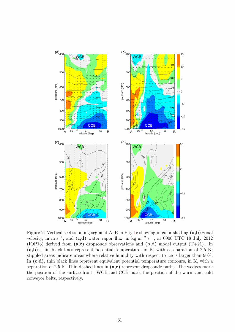
285

290

295

300

305

310

315

latitude (deg)

pres

sure

(hP

a)(a)

WCB

CCB

A B^

56 57 58

400

500

600

700

800

900

1000

-15-10-5051015

285

290

290295

295300

300305

305

310310

315315

pres

sure

(hP

a)

latitude (deg)

(b)WCB

CCB

A B^

56 57 58

400

500

600

700

800

900

1000 −15

−10

−5

0

5

10

15

305

310

310

310

315

315

315

315

315

315

latitude (deg)

pres

sure

(hP

a)

(c)WCB

CCB

A B^

56 57 58

400

500

600

700

800

900

1000

-0.2

-0.1

0

0.1300

305

305

310

310

315

315

315

315

320 320

pres

sure

(hP

a)

latitude (deg)

(d)WCB

CCB

A B^

56 57 58

400

500

600

700

800

900

1000 −0.2

−0.1

0

0.1

Figure 2: Vertical section along segment A–B in Fig. 1c showing in color shading (a,b) zonalvelocity, in m s−1, and (c,d) water vapor flux, in kg m−2 s−1, at 0900 UTC 18 July 2012(IOP13) derived from (a,c) dropsonde observations and (b,d) model output (T+21). In(a,b), thin black lines represent potential temperature, in K, with a separation of 2.5 K;stippled areas indicate areas where relative humidity with respect to ice is larger than 90%.In (c,d), thin black lines represent equivalent potential temperature contours, in K, with aseparation of 2.5 K. Thin dashed lines in (a,c) represent dropsonde paths. The wedges markthe position of the surface front. WCB and CCB mark the position of the warm and coldconveyor belts, respectively.

31

295

300

305

310

315

320

325

latitude (deg)

pres

sure

(hP

a)

(a)

WCB

LLJ

C D^

54 54.5 55 55.5 56

400

500

600

700

800

900

1000

-35-30-25-20-15-10-5

295

295

300300

305305

310

310

315315

320

325

pres

sure

(hP

a)

latitude (deg)

(b)

WCB

LLJ

C D^

54 54.5 55 55.5 56

400

500

600

700

800

900

1000 −35

−30

−25

−20

−15

−10

−5

310

310 310

310

315

315315

320

320

325

325

latitude (deg)

pres

sure

(hP

a)

(c)

WCB

LLJ

C D^

54 54.5 55 55.5 56

400

500

600

700

800

900

1000

-0.4-0.35-0.3-0.25-0.2-0.15-0.1-0.05

305

310

310

315

315

320

320

325

325

325

325

330

pres

sure

(hP

a)

latitude (deg)

(d)

WCB

LLJ

C D^

54 54.5 55 55.5 56

400

500

600

700

800

900

1000 −0.4

−0.35

−0.3

−0.25

−0.2

−0.15

−0.1

−0.05

Figure 3: As in Fig. 2, but for the vertical section along segment C–D in Fig. 1d at 1600UTC 15 August 2012 (IOP14). The model output in (b,d) corresponds to the output of 22-hintegration. LLJ marks the position of a low-level jet. Notice that the colorbars in Fig. 2and here are different.

32

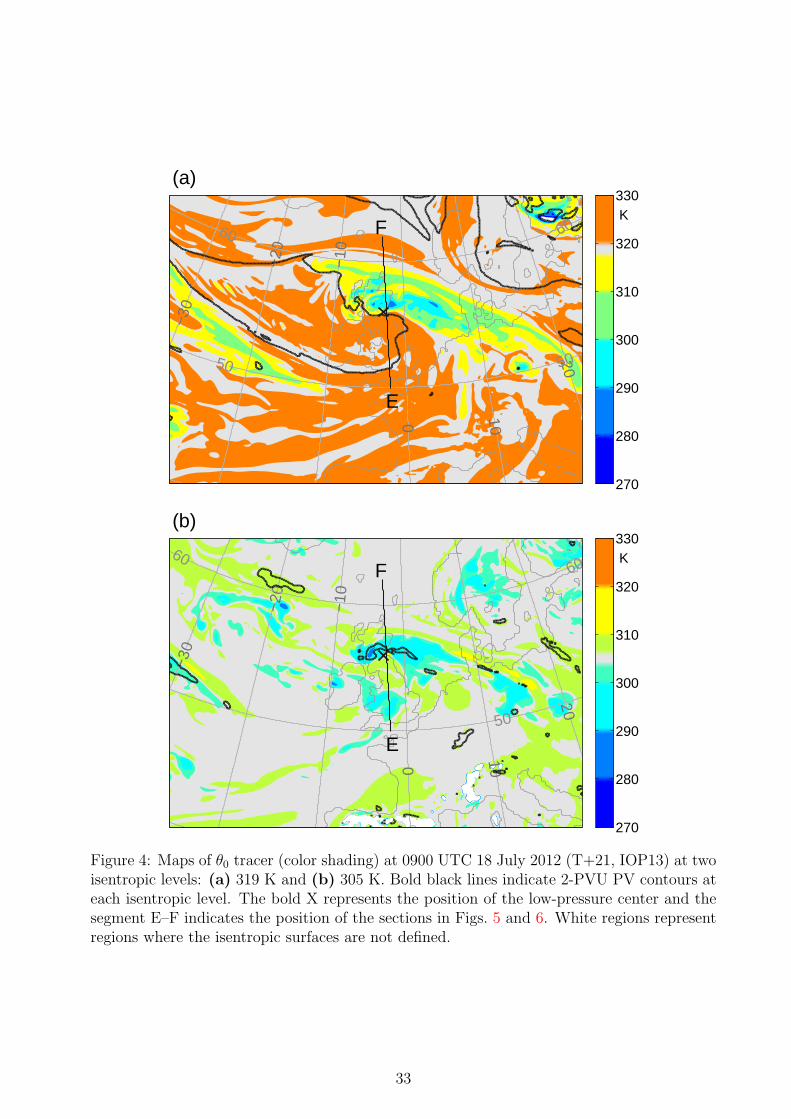
−30

−20

−10

0 10

2050 50

60 60

(a)

E

F

270

280

290

300

310

320

K330

−30

−20

−10

0 10

20

50

6060

(b)

E

F

270

280

290

300

310

320

K330

Figure 4: Maps of θ0 tracer (color shading) at 0900 UTC 18 July 2012 (T+21, IOP13) at twoisentropic levels: (a) 319 K and (b) 305 K. Bold black lines indicate 2-PVU PV contours ateach isentropic level. The bold X represents the position of the low-pressure center and thesegment E–F indicates the position of the sections in Figs. 5 and 6. White regions representregions where the isentropic surfaces are not defined.

33

285

290 290

290295

295300

300305

305

310 310

315

315

320

320

325

325330

pres

sure

(hP

a)

latitude (deg)

distance (km)

E F

(a)

50 52 54 56 58 60 62

−500 0 500

300

400

500

600

700

800

900

1000 270

280

290

300

310

320

330K

285

290 290

290295

295300

300305

305

310 310

315

315

320

320

325

325330

pres

sure

(hP

a)

latitude (deg)

distance (km)

E F

(b)

50 52 54 56 58 60 62

−500 0 500

300

400

500

600

700

800

900

1000 −3

−2

−1

0

1

2

3PVU

Figure 5: Vertical section along segment E–F in Fig. 4 showing in color shading (a) θ0 and(b) total PV modification after 21 hours of integration at 0900 UTC 18 July 2012 (T+21,IOP13). In (b), grid points where PV residual error is larger than 1 PVU or relative PVresidual error is larger than 50% have been masked out (white shading). Thin black linesindicate potential temperature contours, in K, with a separation of 2.5 K. Bold black linesindicate 2-PVU PV contours. Bold red lines indicate the position of the system’s warm(solid) and cold (dashed) fronts. The distance in the upper horizontal axis is the distance tothe cyclone’s center.

34

285

290 290

290295

295300

300305

305

310 310

315

315

320

320

325

325

330pr

essu

re (

hPa)

latitude (deg)

distance (km)

E F

(a)

50 52 54 56 58 60 62

−500 0 500

300

400

500

600

700

800

900

1000

-3-2-10123

285

290 290

290295

295300

300305

305

310 310

315

315

320

320

325

325

330

latitude (deg)

distance (km)

E F

(b)

50 52 54 56 58 60 62

−500 0 500

300

400

500

600

700

800

900

1000

-3-2-10123

285

290 290

290295

295300

300305

305

310 310

315

315

320

320

325

325

330

pres

sure

(hP

a)

latitude (deg)

distance (km)

E F

(c)

50 52 54 56 58 60 62

−500 0 500

300

400

500

600

700

800

900

1000

-3-2-10123

285

290 290

290295

295300

300305

305

310 310

315

315

320

320

325

325

330

latitude (deg)

distance (km)

E F

(d)

50 52 54 56 58 60 62

−500 0 500

300

400

500

600

700

800

900

1000 −3

−2

−1

0

1

2

3PVU

Figure 6: Vertical section along segment E–F in Fig. 4 showing in color shading contributionsto PV modification from (a) BL and turbulent mixing, (b) convection, (c) cloud microphysicsand (d) radiation after 21 hours of integration at 0900 UTC 18 July 2012 (T+21, IOP13).Grid points where PV residual error is larger than 1 PVU and relative PV residual erroris larger than 50% have been masked out. Thin black lines indicate potential temperaturecontours, in K, with a separation of 2.5 K. Bold black lines indicate 2-PVU PV contours.Bold red lines indicate the position of the system’s warm (solid) and cold (dashed) fronts.

35

−30

−10

0 10

20

4040

50

6060

(a)

G

HW

CB1

WCB2

270

280

290

300

310

320

K

330−3

0

−20

−10

0 10

20

4040

50 50

60 60

(b)

G

H

270

280

290

300

310

320

K

330

Figure 7: As in Fig. 4, but for IOP14 at 1500 UTC 15 August 2012 (T+21) at the isentropiclevels (a) 320 K and (b) 305 K. The segment G–H indicates the position of the verticalsections in Figs. 8 and 9. WCB1 and WCB2 indicate the primary and secondary WCBbranches, respectively.

36

290

295295

295

300

300

305

305

310310

315

315

320

320

325 325

330

330

335

340345350

pres

sure

(hP

a)

latitude (deg)

distance (km)

C1C2 C3

C4

G H

(a)

50 55 60

−500 0 500 1000

300

400

500

600

700

800

900

1000 270

280

290

300

310

320

330K

290

295295

295

300

300

305

305

310

310

315

315

320320

325

325

330

330335

pres

sure

(hP

a)

latitude (deg)

distance (km)

C1C2 C3

C4

G H

(b)

50 55 60

−500 0 500 1000

300

400

500

600

700

800

900

1000 −3

−2

−1

0

1

2

3PVU

Figure 8: As in Fig. 5, but for the vertical section along segment G–H in Fig. 7 at 1500UTC 15 August 2012 (T+21, IOP14). Bold red lines indicate the position of the system’soccluded warm (solid) and surface cold (dashed) fronts. Labels C1, C2 and C3 indicate theposition of columns of cross-isentropic ascent. Label C4 indicates the position of a PV tower.

37

290

300

300

310

310

320320

330

330

pres

sure

(hP

a)

latitude (deg)

distance (km)

C1

G H

(a)

50 55 60

−500 0 500 1000

300

400

500

600

700

800

900

1000

-3-2-10123

290

300

300

310

310

320320

330

330

latitude (deg)

distance (km)

C1

G H

(b)

50 55 60

−500 0 500 1000

300

400

500

600

700

800

900

1000

-3-2-10123

290

300

300

310

310

320320

330

330

pres

sure

(hP

a)

latitude (deg)

distance (km)

C1

G H

(c)

50 55 60

−500 0 500 1000

300

400

500

600

700

800

900

1000

-3-2-10123

290

300

300

310

310

320320

330

330

latitude (deg)

distance (km)

C1

G H

(d)

50 55 60

−500 0 500 1000

300

400

500

600

700

800

900

1000 −3

−2

−1

0

1

2

3PVU

Figure 9: As in Fig. 6, but for the vertical section along section G–H in Fig. 7 at 1500UTC 15 August 2012 (T+21, IOP14). Bold red lines indicate the position of the system’soccluded warm (solid) and surface cold (dashed) fronts. Label C1 represents the position ofthe strongest column of cross-isentropic ascent.

38

5 10 15 20280

290

300

310

320

330

340(a)

time (hr)

θ (K

)

5 10 15 20280

290

300

310

320

330

340(b)

time (hr)

θ 0 (K

)

280

290

300

310

320

330

340

time (hr)

θ (K

)

(c)

5 10 15 20295

300

305

310

315

320

325

330

-505101520

time (hr)

(d)

5 10 15 20295

300

305

310

315

320

325

330

−5

0

5

10

15

K20

Figure 10: (a,b) Cross-isentropic mass transport within a 1000-km spherical cap concentricto the cyclone for (a) IOP13 and (b) IOP14. The lines are colored according to the θ0-binwhose PDF they represent. Dashed lines, bold solid lines and thin solid lines represent the2.5th, 50th and 97.5th percentiles of θ values, respectively, identified within each θ0-bin. (c,d)Heating in the bin with 300 < θ0 ≤ 310 [K] in a 1000-km spherical cap concentric to thecyclone for (c) IOP13 and (d) IOP14. Bold lines represent medians; thin lines represent the25th and 75th θ-value percentiles; dotted lines represent the 5th and 95th θ-value percentiles.

39

time (hr)

θ (K

)

(a)

5 10 15 20295

300

305

310

315

320

325

330

-505101520

time (hr)

(b)

5 10 15 20

-505101520

time (hr)

(c)

5 10 15 20

-505101520

time (hr)

(d)

5 10 15 20

-505101520

time (hr)

θ (K

)

(e)

5 10 15 20295

300

305

310

315

320

325

330

-505101520

time (hr)

(f)

5 10 15 20

-505101520

time (hr)

(g)

5 10 15 20

-505101520

time (hr)

(h)

5 10 15 20−5

0

5

10

15K

Figure 11: Heating due to the parametrization of (a,e) BL and turbulent mixing, (b,f)convection, (c,g) cloud microphysics and (d,h) radiation for the bin with 300 < θ0 ≤ 310 [K]in a 1000-km spherical cap concentric to the cyclone for (a-d) IOP13 and (e-h) IOP14. Boldlines represent medians; thin lines represent 25th and 75th θ-value percentiles; dotted linesrepresent 5th and 95th θ-value percentiles

40

−1 0 1 2 3x 10

−4

400

500

600

700

ζθ (s−1)

p (h

Pa)

315

310

305

θ (K

)

(a)

−1 0 1 2 3x 10

−4

400

500

600

700

ζθ (s−1)

p (h

Pa)

310

305

300

θ (K

)

(b)

−1 0 1 2 3x 10

−4

400

500

600

700

ζθ (s−1)

p (h

Pa)

315

310

305

θ (K

)

(c)

−1 0 1 2 3x 10

−4

400

500

600

700

ζθ (s−1)

p (h

Pa)

315

310

305

θ (K

)

(d)

TotalConservedDiabatic

−1 0 1 2 3x 10

−4

400

500

600

700

ζθ (s−1)

p (h

Pa)

315

310

305

θ (K

)

(e)

−1 0 1 2 3x 10

−4

400

500

600

700

ζθ (s−1)

p (h

Pa)

320

315

310

305

θ (K

)

(f)

−1 0 1 2 3x 10

−4

400

500

600

700

ζθ (s−1)

p (h

Pa)

320

315

310

305

θ (K

)

(g)

−1 0 1 2 3x 10

−4

400

500

600

700

ζθ (s−1)

p (h

Pa)

320

315

310

305

θ (K

)

(h)

Figure 12: Vertical profiles of average isentropic vorticity (black) for a 500-km spherical capconcentric to the cyclone for (a–d) IOP13 and (e–h) IOP14: (a) 1500 UTC (T+3) and(b) 2100 UTC 17 July 2012 (T+9); (c) 0300 UTC (T+15) and (d) 0900 UTC 18 July2012 (T+21); (e) 2100 UTC 14 August 2012 (T+3); (f) 0300 UTC (T+9); (g) 0900 UTC(T+15) and (h) 1500 UTC 15 August 2012 (T+21). The frames also show contributionsfrom conserved PV (blue) and diabatically-generated PV (orange), and the value of planetaryvorticity at the position of the cyclone’s center (gray vertical line). The dashed lines representthe conserved and diabatically-generated PV contributions with the contribution from theresidual added and subtracted as an indication of uncertainty.

41

−1 0 1x 10

−4

400

500

600

700

ζθ (s−1)

p (h

Pa)

315

310

305

θ (K

)

(a)

−1 0 1x 10

−4

400

500

600

700

ζθ (s−1)

p (h

Pa)

315

310

305

300

θ (K

)

(b)

−1 0 1x 10

−4

400

500

600

700

ζθ (s−1)

p (h

Pa)

315

310

305

θ (K

)

(c)

−1 0 1x 10

−4

400

500

600

700

ζθ (s−1)

p (h

Pa)

315

310

305

θ (K

)

BLConvMicrophysRad

(d)

−1 0 1x 10

−4

400

500

600

700

ζθ (s−1)

p (h

Pa)

320

315

310

305

θ (K

)

(e)

−1 0 1x 10

−4

400

500

600

700

ζθ (s−1)

p (h

Pa)

320

315

310

305

θ (K

)

(f)

−1 0 1x 10

−4

400

500

600

700

ζθ (s−1)

p (h

Pa)

320

315

310

305

θ (K

)

(g)

−1 0 1x 10

−4

400

500

600

700

ζθ (s−1)

p (h

Pa)

320

315

310

305

θ (K

)

(h)

Figure 13: Vertical profiles of contributions of BL and turbulent mixing processes (BL),parametrized convection (Conv), cloud microphysics processes (Microphys) and radiation(Rad) to average isentropic vorticity for a 500-km spherical cap concentric to the cyclonefor (a–d) IOP13 and (e–h) IOP14: (a) 1500 UTC (T+3) and (b) 2100 UTC 17 July 2012(T+9); (c) 0300 UTC (T+15) and (d) 0900 UTC 18 July 2012 (T+21); (e) 2100 UTC 14August 2012 (T+3); (f) 0300 UTC (T+9); (g) 0900 UTC (T+15) and (h) 1500 UTC 15August 2012 (T+21).

42