MEAN-VALUE PRINCIPLE UNDER CUMULATIVE PROSPECT THEORY

Astin Bulletin 42(1), 103-122. doi: 10.2143/AST.42.1.2160737 © 2012 by Astin Bulletin. All rights reserved.

MEAN-VALUE PRINCIPLEUNDER CUMULATIVE PROSPECT THEORY

BY

MAREK KALUSZKA AND MICHAŁ KRZESZOWIEC

ABSTRACT

In the paper we introduce a generalization of the mean-value principle under Cumulative Prospect Theory. This new method involves some well-known ways of pricing insurance contracts described in the actuarial literature. Properties of this premium principle, such as translation and scale invariance, additivity for independent risks, risk loading and others are studied.

1. INTRODUCTION

From the practical point of view, the mean-value principle is based on a belief that people use a utility function while making decisions under risk and uncer-tainty and they can properly evaluate the probabilities of gains and losses. Gerber (1979), Goovaerts et al. (1984) and Rolski et al. (1999) study the prop-erties of this principle assuming that a value function is convex and twice differentiable. However, in reality, these assumptions are usually incorrect.On the one hand, numerous experiments carried out by Kahneman and Tversky (1979) confi rm the fact that under risk and uncertainty people make decisions using a function which assigns virtual value to monetary outcomes. On the other hand, they notice that people decide which outcomes they see as basically identical and they set a reference point and consider lower outcomes as losses and larger as gains. They suggest replacing the utility function, which measures absolute wealth, with a value function that depends on relative payoff and meas-ures gains and losses. According to them, such a function should be convex for negative and concave for positive arguments.

In addition to this observation, Köszegi and Rabin (2007) notice that mak-ing decisions under uncertainty increases risk aversion if the risk is expected. Reference points, which infl uence decision maker to take certain action under uncertainty, are allocated on the basis of beliefs of a decision maker concerning a possible outcome and they can be determined in a stochastic way. Taking action relies on maximizing the functional EF Ò v (w|r) dG (r), where v is the value function proposed by Kahneman and Tversky, w is the wealth with distribution F and G is a probability distribution function of a discrete random variable R with fi nite support. Under these assumptions we may deal with value function

95371_Astin42-1_05_Kaluszka.indd 10395371_Astin42-1_05_Kaluszka.indd 103 5/06/12 13:525/06/12 13:52

104 M. KALUSZKA AND M. KRZESZOWIEC

v(w) = Ò v (w|r) dG (r) with very irregular shapes, in particular they can be functions which are not differentiable at many points. Gillen and Markowitz (2010) suggest functions which are piecewise convex and concave, thus have some infl ection points, but are differentiable at every point. The analysis of certain subclasses of these functions allows us to determine a decision maker’s willingness to undertake risk. It still remains an issue for debate which typeof a value function corresponds the most to human behavior while making decisions. Therefore, in order to obtain results for possibly large class of value functions, we should put possibly weak assumptions concerning the value function.

Kahneman and Tversky (1979) also discover that people distort probabilities while making decisions under risk and uncertainty. Rank-dependent utility model eliminates the problem of overweighting very small probabilities (e.g. Quiggin 1982). Formalization of this idea relies on distorting the cumulative distribution function, not the single probabilities. Tversky and Kahneman (1992) use the concept of rank-dependent utility model and create Cumulative Pros-pect Theory in which they assume that probabilities of gains and losses are distorted in a different way. This theory has already been widely applied and discussed in many papers (e.g. Schmidt et al., 2008, Teitelbaum, 2007). During last years some authors have adjusted classical theories of fi nance and insurance to Cumulative Prospect Theory (see Schmidt and Zank, 2007, De Giorgi et al., 2009, De Giorgi and Hens, 2006, Bernard and Ghossoub, 2010). In this paper we would like to study a new version of the mean-value principle under Cumulative Prospect Theory.

The paper is organized as follows. In Section 2 we review the mathematical foundations of Cumulative Prospect Theory and defi ne a new version of the mean-value principle adapted to this theory. In Section 3 we analyze properties of this premium principle. Section 4 summarizes the whole article. In the Appendix one may fi nd proofs of theorems and propositions.

2. PREMIUM PRINCIPLE UNDER CUMULATIVE PROSPECT THEORY

In rank-dependent utility model it is assumed that probabilities are distorted by some non-decreasing function g : [0,1] → [0,1] such that g(0) = 0 and g(1) = 1, called probability distortion function (e.g. Segal, 1989). Let G denote the class of all probability distortion functions. For a fi xed g ! G and random variable X, the Choquet integral is defi ned by

gt tg ( ) ( )E X g P1> >0

0

- +3

3

-

P X dt X ,dt=: ^^ ^h h h# #

provided both integrals are fi nite. Further we assume that all random variables are defi ned on some probability space (W, A, P). If X takes fi nite number of values x1 < x2 < … < xn with probabilities P(X = xi ) = pi > 0, then Eg X = x1 +


MEAN-VALUE PRINCIPLE UNDER CUMULATIVE PROSPECT THEORY 105

11

ii = g qn -^ h/ (xi + 1 – xi ), where ik 1=q pk=i +

n/ ; in particular for n = 2 we have EgX = x1 (1 – g(p2)) + g(p2) x2. Further we write X $ 0 if P(X $ 0) = 1 andX ! X2

+ if P(X = s) = q = 1 – P(X = 0), where q ! [0, 1] and s > 0 are arbi-trary. The Choquet integral is additive for comonotonic risks, positively homog-enous, monotonic (i.e. EgX $ EgY if X $ Y a.e.) and Eg(c) = c for all c ! �. Moreover Eg( –X ) = – Eg X, where g(x) = 1 – g(1 – x) is dual distortion function. In the literature we can fi nd some classes of probability distortion functions, e.g. g(p) = ,

( ( ) )p p

p

1 /1+ - g gg

g

g(p) = ,( )p pp1+ - gg

g

g(p) = exp (– (– ln p)g ), g(p) = p +g(p – p2) (see Tversky and Kahneman, 1992, Prelec, 1998, Goldstein and Ein-horn, 1987, Sereda et al., 2010). For g, h ! G we defi ne the generalized Choquet integral as

X .E X Egh g h-+ +-E= X ^ h

It is introduced by Tversky and Kahneman (1992) for discrete random variables and is used to describe the mathematical foundations of Cumulative Prospect Theory. In numerous experiments Tversky and Kahneman notice that proba-bilities of losses are distorted in a different way than probabilities of gains.If h(x) = g(x) = 1 – g(1 – x), then EggX = EgX. Usually, formulas for h are similar to those for g but with different values of coeffi cient g.

Lemma 1. The generalized Choquet integral has the following properties:

W1 Egh 1A = g(P(A));

W2 Egh (cX ) = cEghX for all c $ 0;

W3 Egh ( –X ) = – EhgX;

W4 if X # Y, then Egh X # EghY;

W5 if g(x) $ x and h (x) # x for x ! [0, 1], then Egh X $ EX;

W5’ if g(x) # x and h(x) $ x for x ! [0, 1], then Egh X # EX;

W6 if g(x) = h(x) = x, then Egh X = EX;

W7 Egh c = c for all c ! �;

W8 for all c ! � we have

X X> >s sgE c h P Pg g

c

0

+ - - -h hX ds= ,c+ +E X^ ^^ ^^h hh hh6 @# (1)

c gsg g hE E X c P X P X s ds>h h

c

0

$+ = + --

X + ;^ ^^ ^^h hh hh6 @# (2)

W9 Jensen’s inequality: If u : � → � is non-decreasing, concave and u (0) = 0, then for g, h ! G and arbitrary random variable X such that Egh X exists we have



uu

gh h( ) ( ) ( )E u X u m P m X s g P m X s� m m

0

# $ $-

-

�um

� ,u ds+^ ^^ ^^

^ ^

h hh hh

h h

6 @# (3)

where m = Egh X and u� is the right-sided derivative of u. Moreover, if h(x) $ g(x) or X $ 0, then Egh u (X ) # u (Egh X ).

We introduce a premium principle which is a modifi cation of the mean-value principle adjusted to Cumulative Prospect Theory. Let X be an arbitrary random variable which does not have to be non-negative. Then X should be regarded as a total claim made by the insured, decreased by the possible gain earned from investition. This allows us to consider insurance products involving some investment options such as investment-linked life insurance or variable annuity. In case of non-life insurance it is plausible to study non-negative random variables.

Consider a decision-maker whose reference point is w and who wants to purchase an insurance policy paying out the monetary equivalent of the random outcome X. Further, we call (X – w)+ losses and (w – X )+ gains. If X $ 0, then (X – w) + and (w – X)+ denote catastrophic and non-catastrophic loss, respec-tively. In the latter case there is a direct analogy with stop-loss reinsurance. Assume that u1, u2 : �+ → �+ are some non-decreasing value functions, where u1 measures gains and u2 losses. Let g and h be probability distortion functions of gains and losses, respectively. We propose premium H(X ) for insuring X as the solution of

( (X X XH H g ( .u u w E u E u X wh1 2 1 2- - = - - -+ + + +w - ) ) w )_a _̂ ^ _̂i k h i h h i

(4)

Notice that (4) can be rewritten as

gh( )u w H X E u X- = -w^ ^h h (5)

with non-decreasing function u(x) = u1(x +) – u2 ((– x) +) for x ! �. Gerber (1979) considers a similar equation for premium H(X) under assumptions that the value function u is concave and probabilities are not distorted, i.e. g(p) = h(p) = p. In a more general model Luan (2001) assumes that h = g,g is convex and the value function is concave. Van der Hoek and Sherris (2001) analyze a functional with different probability distortion functions for gains and losses. However, they study only the case when the value functions are linear.

Let us determine the minimum assumptions about u under which the pre-mium defi ned by (5) exists and is determined uniquely. It is commonly accepted that u should be non-decreasing. However, if u was constant on some interval, then the premium could not be determined uniquely. Therefore we assumethat u is increasing. It turns out that u should also be continuous. Otherwise,



equation (5) may have no solutions. Without loss of generality we may assume that u (0) = 0. Further we consider increasing and continuous functions u such that u (0) = 0. To simplify the notation we write u ! U if u satisfi es these three conditions. We also denote u ! U0 if u (x) = cx, u (x) = (1 – e – cx) / a or u (x) = (ecx – 1) / a for x ! � and some a, c > 0.

In the following two examples we determine the premium H (X) if u ! U0.

Example 1. If u (x) = cx, then from W2, W3 and (1) we can rewrite (5) as

(XH X

s s

gh)w

g .

c cE w

c w E X h P X P X ds> >hg 0

- = -

= - -+

w^ ^

^_ ^â

h h

hi hh k6 @#

Finally we have

(XH s s)w

g .E X P X h P X ds> >hg 0= + -^^ ^^hh hh6 @# (6)

Example 2. For u (x) = (1 – e – cx) / d from (1) and W3 we can rewrite (5) as

(XHc

c

-

-s

c

c

-

-1

e

cX

-)gh

g .

e E

E e e h P e P e s ds

1 1

1 > >

w w X

hcw w X w X

0

- =

= - -

- -

- - -+

^

^ ^^ ^^

^ ^

^ ^

h

h hh hh

h h

h h6 @#

From the above and W2 we have

1

g .e P e se P e se ds E e> >(cH X cw cX cw cX cwhg

cX

0- =h+ e) ^^ ^^hh hh6 @#

Thus

(X t>H t>) g .lnc E e P e h P e dt1exp

hcX cX cX

cw

0

= + -^ ^^^

^

h hhh

h

6> @ H# (7)

In a similar way we can derive a formula for H(X) if u (x) = (ecx – 1) / d.

In the next example we will determine the premium if we assume that prob-ability distortion functions are neo-additive weighting functions (see Wakker, 2010, p. 208). Further we denote sup X = sup {t : P(X # t) < 1} and inf X = – sup ( – X ).

Example 3. Let u (x) = x. Assume that g(x) = c + dx, h(x) = a + bx for x ! (0, 1), where b, d $ 0, a, c $ 0, a + b # 1 and c + d # 1. If inf X # 0 # sup X, then from (6) we have



X

(

(

X

X P

) ,

H

d

ds

s s

s

d

)

)

(inf

bP X ds dP X ds

a c d b P X ds

a c w d b X s

a X c X bEX dE

1

1

> >

>

>

(

(

sup infX X

w X

w X

0 0

0

0

= + + -

+ - - - + -

= - - - + -

+ + + - -

-

+ +sup

a c

)

)

-^ ^

^ ^ ^

^ ^ ^

h h

h h h

h h h

6 6

6

@ @

@

# #

#

#

(8)

where w(X ) = min (max (inf X, w), sup X ). If c = 0, 0 # d < 1, inf X = 0 andsup X = w, then H(X) = EX + (1 – d ) (sup X – EX). This premium is analyzed by Kaluszka and Okolewski (2008). If w = 0, b = 1 – a and d = 1 – c, then from (8) we get

(XH c) EX .EX a= + - - -+ + + +sup X ( ) ( )sup X E X- -^ ^h h

If inf X # w # sup X and b = d, then

(XH d d) .sup infa c w a X c X EX= - - - + + +1^ h

3. PROPERTIES OF PREMIUM PRINCIPLE UNDER CUMULATIVE

PROSPECT THEORY

Further we assume that X is an arbitrary random variable, unless it is stated otherwise.

1. Non- excessive loading: inf X # H(X ) # sup X.

This property holds for all u ! U and g, h ! G, which is the consequence of W4 and W7.

2. No unjustifi ed risk loading: H(a) = a for all a ! �.

From W7 it follows that this condition is satisfi ed for all u ! U and g, h ! G.

3. Translation invariance: H(X + b) = H(X ) + b.

Proposition 1. Let u ! U0 and g, h ! G. Then H(X ) is translation invariant for all X and b ! � if and only if h = g.

Proposition 2. Let u ! U0 and g, h ! G. Then H(X ) is translation invariant for all X $ 0 and b $ 0 if and only if h = g or w # 0.



Theorem 1. Let u ! U and g, h ! G be continuous. If H(X ) is translation invariant for w = 0 and some w > 0, then u ! U0 and h = g.

4. Scale invariance: H(aX ) = aH(X ) for all a > 0.

Theorem 2. Let u ! U and g, h ! G.

(i) Let u(x) = cx for some c > 0. If w = 0 or h = g, then H(aX ) = aH(X ) for all a > 0.

(ii) Let h be continuous. If X $ 0 and H(X ) is scale invariant for w = 0, then u (x) = – c (– x)d for x # 0 and some c, d > 0.

(iii) Let g, h be continuous. If H(X ) is scale invariant for w = 0 and all X, then u (x) = – c ( – x)d for x # 0 and some c, d > 0 and u (x) = axb for x > 0 and some a, b > 0.

(iv) If h is continuous and H(X ) is scale invariant for all w $ 0 and all X, then u (x) = cx for some c > 0 and all x ! � and g = h.

5. Additivity for comonotonic risks.

Theorem 3. (i) Let u(x) = cx. If h = g ! G, then H(X) is additive for comonotonic risks. (ii) If u ! U, g, h ! G, h is continuous and H(X), which is the solution of (5), is additive for comonotonic risks for all w $ 0 and all X, then u(x) = cx and h = g.

6. Additivity for independent risks.

Theorem 4. (i) If g(p) = h(p) = p and u ! U, then H(X ) is additive for inde-pendent risks if and only if u ! U0.(ii) Let u ! U0, g, h ! G be such that h (0 +) = 0, h (1 – ) = 1 and there exists left-sided derivative of h at x = 0. If H(X ) is additive for independent risks for w = 0 and some w > 0, then g(p) = h(p) = p.

Notice that in Theorem 4 we do not put any additional requirements on func-tion g. Moreover, from (ii) it follows that in practice it is enough to check the additivity for independent risks for two values of w in order to be certain that probabilities are not distorted.

7. Subadditivity: H(X + Y ) # H(X ) + H(Y ).

Theorem 5. Let u (x) = cx for some c > 0 and h = g, where g ! G. Then H(X ) is subadditive if and only if g is convex.

8. Stop-loss order preserving: X #sl Y implies H(X ) # H(Y ).

Theorem 6. If u ! U is concave, g, h ! G are such that g = h, g is convex and X #sl Y, then H(X ) # H(Y ).



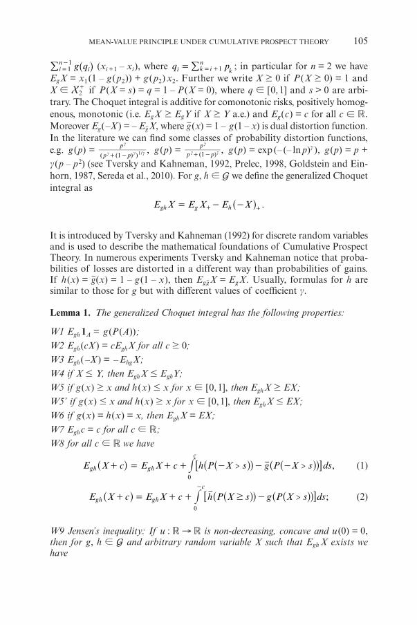
9. Risk loading.

One of the properties characterizing the premium is risk loading, i.e. H(X ) $ E(X ). If this condition is not satisfi ed, then obviously no insurance company would decide to sell the policy. The following propositions describe in terms of rank-dependent utility theory two groups of people: those who either can afford to buy an insurance or refuse to be insured. Generally, risk loading holds if and only if

(X X) ( ) .w u E u wE gh# - -1- ` j (9)

Since it can be diffi cult to evaluate the right-hand side of (9), we give some suffi cient conditions when risk loading is satisfi ed.

Proposition 3. If u ! U is concave and g, h ! G are such that g(x) # h (x) # x for all 0 # x # 1, then H(X ) $ E (X ).

In the next two propositions we assume that X $ 0.

Proposition 4. Assume that u ! U, g, h ! G and X is non-negative, bounded random variable such that w < s = sup X. Then H(X ) $ E (X ) holds, if

(X s s( )=) ( ) ( ) ( ) .E w u g P w u w h P u<1# - + -- X wX^ ^h h6 @ (10)

If X takes only the values from the set {0, w, s}, then (10) is equivalent to H(X) $ E (X ).

Proposition 5. Assume that u ! U and g ! G. Then H(X ) $ E (X ), if

w( ) ( ) ( ) .E w u u w g P <# - 1-X X^_ hi (11)

If P(X = 0) + P(X = w) = 1, then (11) is equivalent to H(X ) $ E (X ).

Example 4. For some types of value functions and probability distortion functions we can check directly when risk loading holds. Let u(x) = x, g(p) = p + g1(p – p2) and h(p) = p + g2(p – p2), where |g1|, |g2| # 1. If g1 # 0, then g is convex and for g1 $ 0 function g is concave. Moreover g(p) – h(p) = – p(1 – p) (g1 + g2). From (6) we have

(X

X X

H

s s

s

s

s s

<$

s

s

$

)

.EX P ds P dsg g= + -

ds-

3-w

( )P X P P X s ds P X s P X s ds

P P P X

P X X P X s

> > >

> >

w

w

20

1 20

10

2 1

# #

# #

g g g

g

= + - +

- + - -

3

3

3

X

X

^ ^ ^ ^ ^

^ ^ ^

^ ^ ^ ^

h h h h h

h h h

h h h h

6

6

@

@

# #

#

# #



Thus H(X ) $ EX if and only if

P P3-w

.X s P X s ds X s P X s ds> >w

1# $ #g g3

2 ^ ^ ^ ^h h h h# #

This condition is satisfi ed for example if g2 $ 0 and g1 # 0. Let X = max (X, w), X = min (X, w). Notice that if X and X� are i.i.d. random variables, then

s>

=

s

E

w

+

P X s P X s ds E X ds

E X X X X21

>w

1 1# #=

= -

3 3

-� �

X�

,

^ ^ ^ ^

^

h h h h

h

# #

which is known as Gini coeffi cient.

In a smilar way we prove that E3-

.P X s P X s ds X X21>

w

# = -�^ ^h h# Since

| x – y | = 2max (x, y) – x – y, we have

(X E:2 2H E-) EX X X X X2 1g g= + - -:2 2E ,E^ ^h h

where X2:2 = max (X, X�) and X 2:2 = max (X , �X ).

4. CONCLUDING REMARKS

We have presented a new version of premium principle under Cumulative Prospect Theory. This premium principle satisfi es non-excessive and no unjus-tifi ed risk loading conditions for all types of value functions and probability distortion functions. It is translation invariant only if the value function is linear or exponential and h = g. Scale invariance and additivity for comonotonic risks are satisfi ed if the value function is linear and h = g. Additivity for independent risk holds if the value function is linear and exponential and probabilitiesare not distorted which corresponds to the case described by Gerber (1979). If the value function is linear and h = g, then the principle is subadditive if and only if g is convex. In general this premium principle does not satisfy risk loading, but we give some conditions under which this property holds. This paper extends results by Gerber (1979), Van der Hoek and Sherris (2001) and Luan (2001) under mild assumptions on considered functions. The results are obtained by examining functional equations instead of differential equations.

ACKNOWLEDGEMENT

The authors would like to thank anonymous referees for their valuable com-ments and suggestions to improve the paper and clarify its presentation.



Michał Krzeszowiec acknowledges the fi nancial support of the National Science Centre (“Analysis of premium principles under Kahneman-Tversky Theory”, Grant No. 2011/01/N/HS4/05627).

APPENDIX

Proof of Lemma 1. Proofs of W1, W3 and W6 are obvious. Proofs of W2, W5, W5’ and W7 are the consequence of the defi nition of the generalized Cho-quet integral, the Choquet integral and properties of the Choquet integral.

Ad W4 If X # Y, then P(X > t) # P(Y > t) for t ! �. Thus

.Yg +gE g P X t dt P Y t dt E> > g0 0

= =3 3

+X #^^ ^^hh hh# #

Moreover, if X # Y, then –Y # – X and P(–Y > t) # P(–X > t) for t ! �. Hence Eh(–X ) + $ Eh(–Y ) +.

Ad W8 Firstly, we will prove (1). We have

hc

g h

g h

g h

c- c

cc-

g

E X c g P t dt P X t c dt

P X t dt P X t dt

E P X t dt P X t dt

E X P X s ds P X s ds

E c h P X s P X s ds

> >

> >

> >

< >

> >

gh

gh

gh

c c

gh

c

0 0

0 0

0 0

0

+ = - - - +

= - -

= - -

= - + -

= + + - - -

3 3

3 3

,X

X

+

X +

^ ^^ ^^

^^ ^^

^^ ^^

^^ ^^

^^ ^^

h hh hh

hh hh

hh hh

hh hh

hh hh6 @

# #

# #

# #

# #

#

because the modifi cation of values of the integrated function at a countable number of points yields

c cg gP X s ds P X s ds> #- = -0 0

^_ ^_hi hi# # . Formula (2) is obtained from (1) after making some elementary calculations.

Ad W9 Obviously u (x) # u (m) + u�(m)(x – m) for all x, where u� is the right-sided derivative of u. From this, W2, W4 and (2) we have

( ) ( )m m

gh

h

� �( ) ( ) ( ) ( )

( )

E E u m u m m u m X

u m P X s g P X s ds�( ) ( )

gh

u m m u m

0

#

$ $

- +

= -

-

Xu

� �u u+ ^^ ^^hh hh

6

6

@

@#



and we get (3). Moreover u�(m) m – u (m) # 0 and u (0) = 0, so if h $ g,then Egh u (X ) # u (Egh X ). If X $ 0, then P(u�(m) X $ s) = 1, hence Egh u (X) # u (Egh X ). ¡

Proof of Proposition 1. Let u (x) = cx. From (6) and W8 we have

b

s s

b .ds+

g

g

( )H b E b h P X P X ds

P X s h P s

> >

> >

hg

b

w0

0

+ = + - - -

- - -

X X

X

+ ^^ ^^

^^ ^^

hh hh

hh hh

6

6

@

@

#

#

Hence H(X + b) = H(X ) + b for all b ! � if and only if

(12)

b s b

g

g g .

h P X s P X s ds

P s P s h P h P s ds

> >

> > > >

b

w0

0

- - -

= - - - - -X X X X

^^ ^^

^_ ^^ ^^ ^^_

hh hh

hi hh hh hhi

7

6

A

@

#

#

Clearly, if h = g, then H(X ) is translation invariant. Suppose now that h(z) !g(z) for some z. Let b > w $ 0 and X be the random variable such that P(X =– s0) = z = 1 – P(X = 0), where b – w < s0 < b. Then (12) can be rewritten as

( (

gz

s-

g g) )

.

h z z s h z z dt

h z w b s

w b

0

0

0

- = - - -

= - - - - +

-

1 1

1 1

^ ^

^ ^_ _

h h

h hi i

6 6@ @#

Since (h (z) – g(z))s0 ! 0, we get a contradiction that b is arbitrary such that max (s0, w) < b < s0 + w. For w < 0 let b < w and let X be such that P(X = s0) =z = 1 – P (X = 0), where 0 < w – b < s0 < – b. Then (12) can be rewritten as

w b+g g( ) ( )s z h z h z z0 0- - - = - -1 s1 ,^ ^^ ^ ^h hh h h

which contradicts that b is arbitrary such that w – s0 < b < min (– s0, w).Let u (x) = (1 – e – cx) / a. From (7) under b > w $ 0 we have

s>sg( ) .lnH b c E P h P ds b1 >

( ( ))exp

hcX cX cX

c w b

0

+ = - +

-

X e ee + ^^ ^^hh hh6> @ H# (13)

If h = g, then H(X + b) = H(X) + b for all b ! �. Suppose that g(z) ! h(z) for some z. Let X be such that P(X = s0) = 1 – z = 1 – P(X = 0), where s0 < w – b < 0. Then



s s> >

b

g g !( ) ( ) ( ) ( ) 0P h P ds z h z e( ( ))

( )exp

cX cXc

cs c w b

0

0- = - - -ew-

e e^ ` ^ ^h j h h9 C#

and from (13) and (7) it follows that H(X) is not translation invariant. An analo-gous proof can be carried out for u (x) = (ecx – 1) / d. ¡

Proof of Proposition 2. Since P (X > t) = 1 for t < 0 and g(1) = h(1) = 1, then for b $ 0 we have

b h-g g

g .

P s P X s b ds P X t h P X t dt

P t h P X t dt

> > > >

>

w

b

w b

w b0

0

- - = -

=

-

-

-

-

X

X >

^_ ^_ ^^ ^^

^^ ^^

hi hi hh hh

hh hh

6 6

6

@ @

@

# #

#

Notice that Ehg(X + b) = Ehg X + b, because X + b $ 0. Hence for u(x) = cx from (6) it follows that

g( ) .H X b H h P X s P X s ds> >w b

w

+ = -- +

X + b +^ ^^ ^^

^

h hh hh

h

6 @# (14)

From (14) it follows that if w # 0 or g = h, then H(X + b) = H(X) + b. Suppose that w > 0 and g(z) ! h(z) for some z. Let b > w and X be such that P(X = s0) =z = 1 – P (X = 0), where 0 < s0 < w. Then

g ( )z+

g !0,h P X s P X s ds s> >w b

w

0- = --

( )h z^_ ^^ ^

^

hi hh h

h

8 B#

which means that H(X ) is not translation invariant.If u (x) = (1 – e – cx) / d, then from (7) and (13) for b > 0 we have

s s>e

g( ) .lnH b c E P h P ds b1 >hcX cX cX

0

(c

+ = + - +X

)w b-

e e e_` ^îj hh9> C H#

If w # 0 or g = h, then H(X ) is translation invariant because ec(w – b) < 1 forb $ 0 and ecX $ 1. Let w > 0 and g(z) ! h(z) for some z. For random variable X such that P(X = s0) = z = 1 – P(X = 0), where 0 < s0 < w – b we get

s>s>g g !( ) ( ) 0P h P ds e z h z1cX cXe

cs

0

( )c w b

0- = - -

-

,e e_` ^` ` îj hj j h9 C#



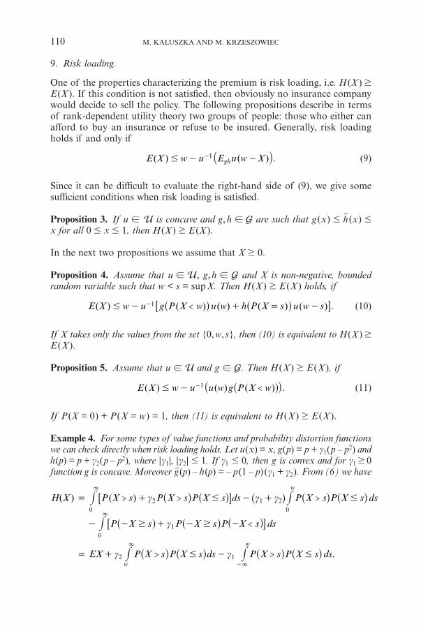
which means that H(X ) is not translation invariant. An analogous proof can be carried out for u (x) = (ecx – 1) / d. ¡

Proof of Theorem 1. Assume that H(X + b) = H(X) + b for all b $ 0. Consider X ! X2

+. Then from (5) under w = 0 we have

E =( ) ( ) ( ) ( ) ( ) .u H u E u u s h qgh h- = - = - - - -+X X X^ ^h h

Thus

(q) ( )( )

.h u su H

=-

- X^ h (15)

Since H(X ) = 0 for q = 0 and H(X ) = s for q = 1, from the monotonicity and continuity of u and h it follows that H(X ) is continuous and non-decreasing function of variable q, thus it takes all values from [0, s ]. From the translation invariance of H(X ), we can rewrite (5) for X + b as

( ) ( ) ( )

( ) ( ) ( ) ( ) .

u H b E u X b E u X b

u b h q u s b h q1

gh h- - = - - = - - - -

= - - + - -

+X^ ^

^

h h

h (16)

Putting (15) into (16), denoting x = – H(X ), y = – b and dividing both sides of obtained equation by u (x) u (– s), we get

( , ( ,f x y f s y= -) ) (17)

for all y # 0, s > 0 and – s # x # 0, where f (x, y) = (u(x + y) – u (y)) / u (x). Setting s = 1 in (17) yields

( , ( ,f x y f y1= -) ) (18)

for y # 0, – 1 # x # 0. Putting x = – 1 in (17) gives

( , ( ,f y f ys 1= -- ) ) (19)

for y # 0 and – s # – 1. From (18) and (19) we have f (x, y) = f (– 1, y) for allx, y # 0. Hence for a fi xed y we have

( (y( ) ) ( ) )u c u x u+ = +x y y (20)

for all x # 0, where c(y) is some function. By the symmetry we have

( ( () ( ) ) ( ) ) ( )c u x u c x u u x+ = +y y y



for x, y # 0, which is equivalent to

( () 1 ( ) ( ) )c u x c x u1- = -y y^ ^h h (21)

for x, y # 0. If c(y) ! 1 for all y < 0, then

((

( )( )

) 1)

c xu x

cu

1-=

-yy

for x, y # 0. Hence u (x) = d (c (x) – 1) for some d > 0 and from (20) we get

(y( ) ( ) )c c x c+ =x y (22)

for x, y # 0. Since u(x) = d (c(x) – 1) and u ! U, it follows that c is continuous and increasing if d > 0. Thus the only solution of (22) is c(x) = eax for x # 0 and some a > 0 (see Kuczma, 2009, p. 349). Hence the only solution of (20) is u (x) = d (eax – 1) for x # 0. If d < 0, then using a similar reasoning we get u (x) = (1 – e – ax) / d, where a > 0. If c (y) = 1 for some y, then from (21) it fol-lows that c (x) = 1 for x # 0. From (20) and continuity of u it follows that u(x) = ax for x # 0.

We will show that u is linear or exponential on � and h = g. Rewriting (5) for X ! X2

+, from the translation invariance of H(X ) we have

q( ) ( ) (1 ) ( ) (u H b u w b g u w s b h- = - - + - -X qw - )^ h (23)

if b # w # b + s and

b( ) ( ) (1 ( )) ( ) ( )u H u w b h q u w s b h q- = - - + - -Xw -^ h (24)

for b $ w. Let u (x) = cx for x < 0. For b > w from (24) we have H(X ) = sh (q). For q0 ! (0, 1) such that h(q0) = 1/2, s = 2(w – b) and H(X ) = sh(q0) from (23) we get u (x) = c1x for x > 0, where c1 = c / (2g(1 – q0)). Setting s = w – b in (23) yields g = h and c1 = c. Now, let u(x) = (1 – e – cx) / a for x < 0. From (24) we have H(X ) = c

1 ln (ecsh(q) + (1 – h (q))). Putting s = ln (2ec(w – b) – 1) / c and the formula for H(X ) with q0 into (23) gives u (x) = (1 – e – cx) / a1 for x > 0, where a1 = 2ag (1 – q0). In order to prove that u (x) = (1 – e – cx) / a for x $ 0 and h = g we use a similar reasoning as in the previous case. An analogous proof can be carried out for u (x) = (ecx – 1) / a. ¡

Proof of Theorem 2. (i) If u (x) = cx, then from (6) for a > 0 we have

w

s s

g

g

( ) ( ) / /

.

H a E a P X s a h P X s a ds

a a P h P ds

> >

> >/

hg

w

hg

a0

0

= + -

= + -

X X

E X X X

^_ ^_

^^ ^^

hi hi

hh hh

7

6

A

@

#

#



If w = 0 or h = g, then H(X ) is scale invariant.

(ii) Assume that H(aX ) = aH(X ). For X ! X2+ from (5) under w = 0 we have

( ) ( ) ( )u a h q u as- = -y (25)

for all a > 0, where y = H(X ). Setting f (x) = – u (– x) and determining h (q) from (25) with a = 1, we can rewrite (25) as

((

) ( ) ( ))

f a f as f sf

=yy

(26)

for all s > 0 and 0 # y # s. If we put s = 1 in (26) and divide both sides of this equation by u (– 1), we get z(ay) = z(a) z(y) for all 0 # y # 1 and a > 0, where z(x) = f(x) / (– u(– 1)). Setting y = 1 in (26) yields z(a) z(s) = z(as) for s $ 1 and a > 0. From the last two equations we have z(ax) = z(a) z(x) for all x > 0 and a > 0. By the continuity of z we get z(x) = xd for all x $ 0 and some d > 0(see Kuczma, 2009, p. 349). Hence u (x) = – c(– x)d for all x # 0, some c =– u (– 1) > 0 and d > 0.

(iii) The formula for u (x) if x # 0 follows from (ii). Assume that H (aX ) =aH (X ). Let X be such that P(X = – s) = q = 1 – P(X = 0), where s > 0 and q ! [0, 1] are arbitrary. From (5) under w = 0 we have

( ) ( ) ( )u a g q u as=y (27)

for all a > 0, where y = – H(X ). If we determine g(q) from (27) with a = 1 and put this expression into (27), we obtain again equation (26) with f (x) = u(x). Hence u (x) = axb for x $ 0 and some a, b > 0.

(iv) From the scale invariance of H(X ) and (5) we have

( ) ( ) (1 ) ( ) ( )u w aH u w g q u w as h q- = - + -X^ h (28)

when a $ w / s and

( )aH ( ) ( ) ( ) ( )u X u w g q u w as g q1 1 1- = - + - - -w^ ^h h (29)

if 0 # a < w / s. Setting as = 2w in (28) and choosing q0 ! [0,1] such that H(X ) = s / 2, from (ii) it follows that u (w) = cwdh(q0) / (1 – g(q0)). Thus u (x) =c1xd for x $ 0 and some c1 > 0. Putting this into (29), differentiating both sides of (29) with respect to a and setting a = 0 we get H(X ) = sg(q). If we put H(X) = sg(q), a = 1 and w = s into (29), we obtain (1 – g(q))d = (1 – g(q)). Thus d = 1. Putting w = 0 into (28) yields H(X) = sh(q). Since H(X) = sg(q), we have g = h. As c1 = ch (q0) / (1 – g(q0)) and h(q0) = 1/2, we obtain c = c1. ¡



Proof of Theorem 3. (i) Let u (x) = cx. If h = g, then H(X ) = EgX and the additivity of the Choquet integral for comonotonic risks ends the proof of (i).(ii) If H(X ) is additive for comonotonic risks, then it is scale invariant. From Theorem 2 it follows that u (x) = cx and h = g. ¡

Remark 1. From the proofs of Theorem 2 (iv) and Theorem 3 (ii) it follows that it is enough to assume that X ! X2

+.

Lemma 2. If the domain of u is ,0 218 B, then the solution of

( ) 2 ( )u x x2 = u (30)

is u(x) = xh(ln x), where h is a periodic function with period ln 2 and 0 · h(– 3) = 0. If we additionally assume that u has right-sided derivative at x = 0 (we allow u+(0) = 3), then the only solution is u (x) = cx for some c > 0.

Proof. Putting x = 0 in (30) implies u (0) = 0. Let u be a solution of (30). It is easy to check that h(t) = e– t u (et) is periodic with period ln 2. Setting x = et we have u (x) = xh (ln x) for x > 0, where h is an arbitrary periodic function with period ln 2. Since u has the right-sided derivative at x = 0 and

� ( )( )

lim lim lnu xu x

h x0x x0 0

= =" "

+ +,^ h

h is constant, as a periodic function which has the limit in – 3. ¡

Proof of Theorem 4. (i) The proof will be carried out basing on the idea by Gerber (1979). Let X be an arbitrary risk and Y be constant, i.e. P(Y = d ) = 1 for some d > 0. As H(X ) satisfi es no unjustifi ed risk loading, then from the additivity for independent risk it follows that H(X ) is translation invariant. From Theorem 1 we conclude that u ! U0.

(ii) Let u (x) = cx and w = 0. Assume that H(X ) is additive for independent risks. Assume that X, Y ! X2

+ are independent random variables such that P(X = 1) = p, P(Y = 1) = q. Then

( Yh( ) ), ( (H p H h= =X q),) (31)

Y p q pq pq+ -( ) ( ) ( ) .H X h h+ = + (32)

Since H(X ) is additive for independent risk, from (31) and (32) it follows that

(p q pq h+ - pq( ) ( ) ) (h h p h+ = + q) (33)

for all 0 # p, q # 1. Put q = c – p, where 0 # c # 1. Let (pn)n ! � be the sequence such that p0 = c

2 and pn + 1 = pn(c – pn). Then (pn)n ! � is generated by logistic difference equation (see Polyanin, Manzhirov, 2007, p. 875). From (33) we have



n1 ... 2 / .h p h p h p h p h c 2n n n1+ = + = =+ +c - c -^ ^ ^ ^ ^h h h h h (34)

As pn + 1 / c = c · pn / c · (1 – pn / c), where c # 1, thus p0.lim

n cn =

"3 Hence = .lim 0

n n"3p

Function h is continuous at 0 and at 1, thus letting n " 3 in (34) yields h(c) =2h(c / 2) for all 0 # c # 1. Since h has right-sided derivative at 0 (we allow h�(0) = 3), from Lemma 2 it follows that h(p) = p. We will prove that g(p) = p. Let w > 0 be such that H(X ) is additive for independent risks. Let X, Y ! X2

+ be independent random variables such that P(X = 2w / 3) = 1 , P(Y = 2w / 3) = q. Then for h(x) = x from (6) we have

Y( q s( ) , ) ( ) ,H w H qw ds32

32

, /

w

w0

0 2 31= = -X g ( )q+ 6 6@ @# (35)

Y q s( (1 ) ( ) .H X w q ds32

2 /3, 4 /3

w

w w0

1+ = + + -g ( )q) 6 6@ @# (36)

From (35), (36) and the additivity for independent risks we get

q qs( ) ( ) .ds s ds0,2 /3 2 /3, 4 /3

w

w

w

w w0 0

1 1- = -g g( ) ( )q q6 66 6@ @@ @# #

Thus 2w (g(q) – q) = w (g(q) – q). Hence g(q) = q and fi nally g(q) = q.Now, let u (x) = (1 – e – cx) / d and X, Y ! X2

+ be independent random vari-ables such that P(X = s) = p, P(Y = s) = q. From (7) under w = 0 we get

Y

( (

(

( (

h q

h

( ( (h q

pq

( ) 1 ) ) ( ) ) ) ,

1 ) ( ) )) ) .

ln ln

ln

H c h p h p e H c e

H X Y c p q pq e h p q h pq h pq e

1 1 1

1

cs cs

cs cs2

= - + = - +

+ = - + - + + - - +

X ,

^ h

6 6

6

@ @

@

Additivity for independent risks yields

( ( ( (

( ( ( (

( )q(1 ))(1 ) ) ( ) 2 ) ( ) ) ( )

1 ) ) ) ) .

h p h e h p h q h p h q e h p h q

h p q pq e h p q pq h pq h pq e

cs cs

cs cs

2

2

- - + + - +

= - + - + + - - +

^

^

h

h

We obtained equality of two polynomials of variable ecs. If we compare coef-fi cients of these polynomials, we will get (33). Thus h(x) = x. Let w > 0 be such that H(X ) is additive for independent risks. For p = 1 we have

( )H Y = ln,s q= g( ) 1 ( ) ( ) ,H c q e q q t dt1,

cse

e0

0

cw

cs1- + - -X 6> 6@ H@# (37)



Y ) q g(q)( ( ) ( ) .lnH c e e q t dt1,

cs cse

e e2

0

cw

cs cs21+ = - + q -1 -X 6> 6@ H@# (38)

From (37), (38) and the additivity for independent risks it follows that

g g( ) ( ) ( ) .q dt q t dt, ,

e

e

e

e e0

00

cw

cs

cw

cs cs21 1( )t -q q- =6 66 6@ @@ @# #

Thus g(q) = q and fi nally g(q) = q. An analogous proof can be carried out for u (x) = (ecx – 1) / d. ¡

Proof of Theorem 5. Let u (x) = cx. Then from (6) we have H(X ) = Eg X. Assume that g is convex. It is known that Eg(X + Y) # EgX + EgY if and only if g is concave (see Denneberg, 1994). Thus for g, which is concave, we have

Y Y( ) ( ) ( ) ( ) .H E E X E Y H H Yg g g#+ = + + = +XX X (39)

Assume now that H(X) is subadditive. Then (39) holds, hence g is concave. ¡

Proof of Theorem 6. Let g = h and X #sl Y. Then Eg [– u(w – X)] # Eg [– u(w – Y )]. Hence Eg [u (w – X )] $ Eg [u (w – Y )], because Eg [– u (X )] = – Eg [u (X )]. By the defi nition of H(X ) we have

YY g g( ( ) ) ( ) .u H E u E u H#= =X X-) (uw - w w -w -^ ^h h6 6@ @

From the monotonicity of u we get H(Y ) $ H(X ). ¡

Proof of Proposition 3. From W9 we have

)X(gh( ( )) ( )) ( ),u H E u Egh #=X Xu w -w - ( -w

Thus from W3 and (1) we get

s h sg( ) ( ) ( ) .H E P X P X ds> >hg

w

0

$ -X X + ^ ^h h6 @#

Since g(x) $ h(x) $ x, from W5 it follows that H(X ) $ Ehg X $ E(X ). ¡

Proof of Proposition 4. Put Y = 0 if X < w, Y = w when w # X < s and Y = s if X = s . Since Y # X, from the monotonicity of the generalized Choquet integral we obtain



Y

s

gh( ( )) ( ) ( )

( ( )) ( ) ( ( )) ( ) .

u H E u E u

g P X w u w h P X u w s<

gh#=

= + = -

X X -w w-w -

From the above and (10) it follows that H(X ) $ E (X ). ¡

Proof of Proposition 5. Put Y = 0 for X < w and Y = w for X $ w. Then X = Y if and only if P(X = 0) + P(X = w) = 1. Since Y # X, then

Ygh( )H X( ) ( ) )

( ( )) ( ) .

u E u E

g P X w u w<

g#=

=

X (uw w w- - -

From the above and (11) we have H(X ) $ E (X ). ¡

REFERENCES

BERNARD, C. and GHOSSOUB, M. (2010) Static portfolio choice under Cumulative Prospect Theory. Mathematics and Financial Economics 2, 277-306.

DENNEBERG, D. (1994) Lectures on Non-additive Measure and Integral. Kluwer Academic Pub-lishers, Boston.

GERBER, H.U. (1979) An introduction to Mathematical Risk Theory. Homewood, Philadelphia.GILLEN, B.J. and MARKOWITZ, H.M. (2010) A Taxonomy of Utility Functions. Variations in Eco-

nomic Analysis, Springer New York, 61-69.DE GIORGI, E., HENS, T. and RIEGER, M.O. (2009) Financial Market Equilibria with Cumulative

Prospect Theory. Swiss Finance Institute Research Paper No. 07-21.DE GIORGI, E. and HENS, T. (2006) Making prospect theory fi t for fi nance. Financial Markets

and Portfolio Management 20, 339-360.GOLDSTEIN, W.M. and EINHORN, H.J. (1987) Expression theory and the preference reversal phe-

nomenon. Psychological Review 94, 236-254.GOOVAERTS, M.J., DE VYLDER, F. and HAEZENDONCK, J. (1984) Insurance Premiums: Theory

and Applications. North-Holland, Amsterdam.VAN DER HOEK, J. and SHERRIS, M. (2001) A class of non-expected utility risk measures and

implications for asset allocation. Insurance: Mathematics and Economics 28, 69-82.KAHNEMAN, D. and TVERSKY, A. (1979) Prospect theory: An analysis of decisions under risk.

Econometrica 47, 313-327.KALUSZKA, M. and OKOLEWSKI, A. (2008) An extension of Arrow’s result on optimal reinsurance

contract. Journal of Risk and Insurance 75, 275-288.KÖSZEGI, B. and RABIN, M. (2007) Reference-Dependent Risk Attitudes. American Economic

Review 97, 1047-1073.KUCZMA, M. (2009) An Introduction to the Theory of Functional Equations and Inequalities.

Second edition, Edited by Attila Gilányi, Birkhäuser. Berlin.LUAN, C. (2001) Insurance premium calculations with anticipated utility theory. ASTIN Bulletin

31, 23-35.POLYANIN, A.D. and MANZHIROV, A.H. (2007) Handbook of Mathematics for Engineers and

Scientists. Chapman & Hall / CRC Press, Boca Raton – London.PRELEC, D. (1998) The probability weighting function. Econometrica 66, 497-527.QUIGGIN, J. (1982) A theory of anticipated utility. Journal of Economic Behavior and Organization 3,

323-343.ROLSKI, T., SCHMIDLI, H., SCHMIDT, V. and TEUGELS, J. (1999) Stochastic Processes for Insurance

and Finance. John Wiley & Sons, New York.



SCHMIDT, U., STARMER, C. and SUGDEN, R. (2008) Third-generation prospect theory. Journal of Risk and Uncertainty 36, 203-223.

SCHMIDT, U. and ZANK, H. (2007) Linear cumulative prospect theory with applications to port-folio selection and insurance demand. Decisions in Economics and Finance 30, 1-18.

SEGAL, U. (1989) Anticipated utility theory: a measure representation approach. Annals of Opera-tions Research 19, 359-373.

SEREDA, E.N., BRONSHTEIN, E.M., RACHEV, S.T., FABOZZI, F.J., WEI SUN and STOYANOV, S.V. (2010) Distortion Risk Measures in Portfolio Optimization. In Handbook of Portfolio Con-struction: Contemporary Applications of Markowitz Techniques. Edited by Guerard J.B., 649-673.

TEITELBAUM, J. (2007) A unilateral accident model under ambiguity. Journal of Legal Studies 36, 431-477.

TVERSKY, A. and KAHNEMAN, D. (1992) Advances in prospect theory: Cumulative representation of uncertainty. Journal of Risk and Uncertainty 5, 297-323.

WAKKER, P.P. (2010) Prospect Theory: For Risk and Ambiguity. Cambridge University Press.WANG, S. (1996) Premium calculation by transforming the layer premium density. ASTIN Bul-

letin 26, 71-92.

MAREK KALUSZKA 1)

E-mail: [email protected]

MICHAŁ KRZESZOWIEC 1) 2)

E-mail: [email protected]

1) Institute of Mathematics Łódz University of Technology Ul. Wólczanska 215 90-924 Łódz Poland

2) Institute of Mathematics Polish Academy of Sciences Sniadeckich 8 P.O. Box 21 00-956 Warszawa Poland


Documents

MEAN-VALUE PRINCIPLE UNDER CUMULATIVE PROSPECT THEORY