ME 563 Mechanical Vibrations

Lecture #10 Single Degree of Freedom

Free Response

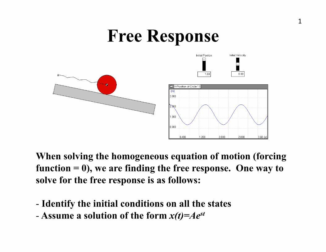
Free Response 1

When solving the homogeneous equation of motion (forcing function = 0), we are finding the free response. One way to solve for the free response is as follows:

-  Identify the initial conditions on all the states -  Assume a solution of the form x(t)=Aest

Disc on An Incline 2

Consider the disc on an incline with no forcing function:

Recall xd is called the dynamic displacement.

If we make a solution of the form, , we obtain:

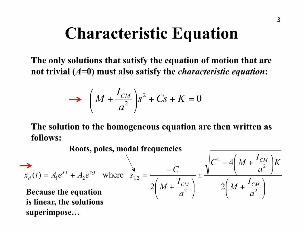
Characteristic Equation 3

The only solutions that satisfy the equation of motion that are not trivial (A=0) must also satisfy the characteristic equation:

The solution to the homogeneous equation are then written as follows:

Roots, poles, modal frequencies

Because the equation is linear, the solutions superimpose…

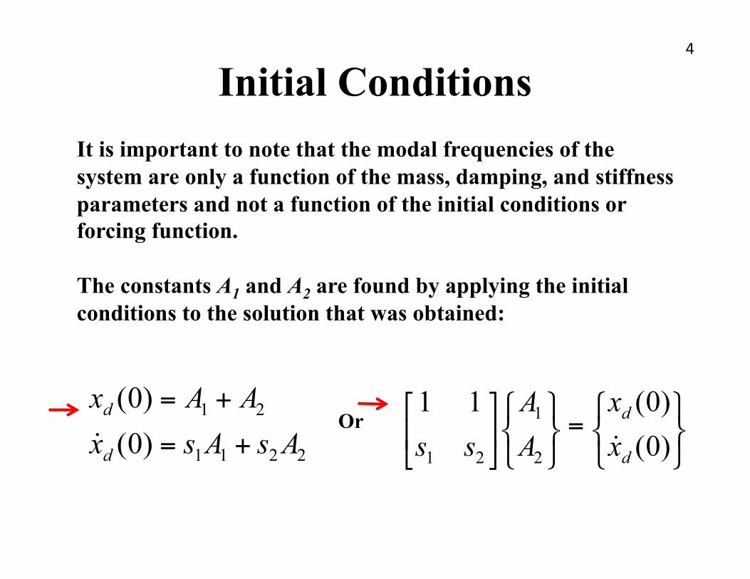
Initial Conditions 4

It is important to note that the modal frequencies of the system are only a function of the mass, damping, and stiffness parameters and not a function of the initial conditions or forcing function.

The constants A1 and A2 are found by applying the initial conditions to the solution that was obtained:

Or

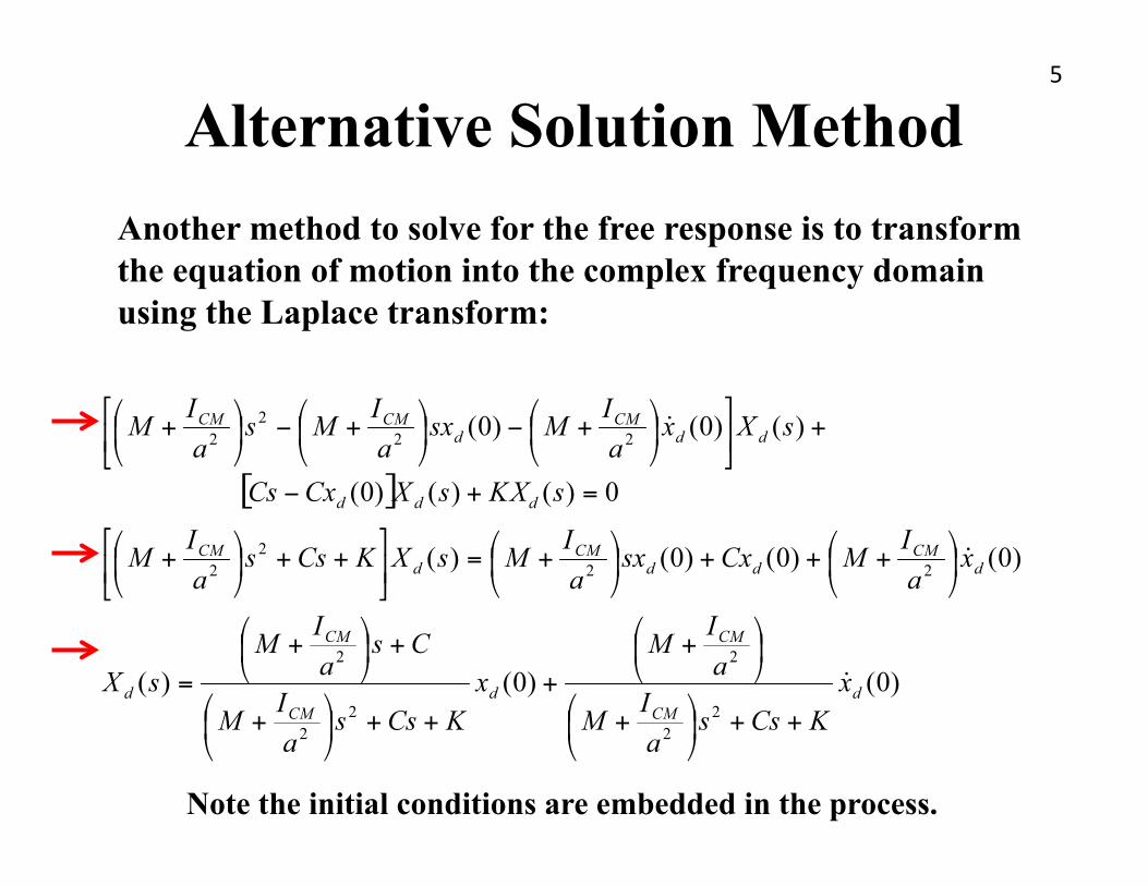
Alternative Solution Method 5

Another method to solve for the free response is to transform the equation of motion into the complex frequency domain using the Laplace transform:

Note the initial conditions are embedded in the process.

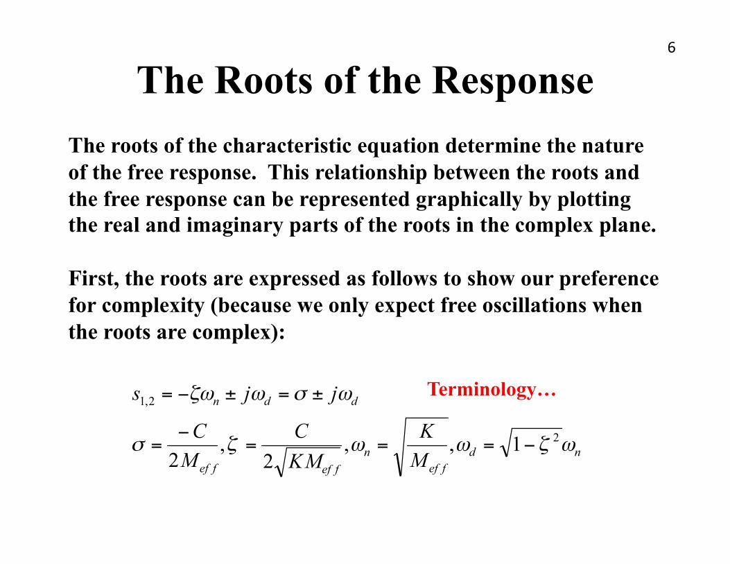
The Roots of the Response 6

The roots of the characteristic equation determine the nature of the free response. This relationship between the roots and the free response can be represented graphically by plotting the real and imaginary parts of the roots in the complex plane.

First, the roots are expressed as follows to show our preference for complexity (because we only expect free oscillations when the roots are complex):

Terminology…

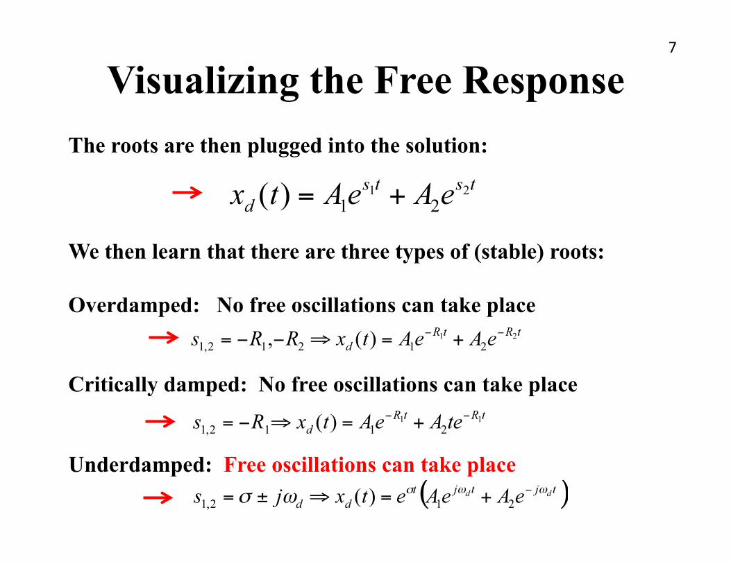
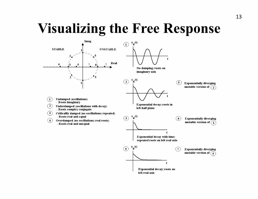
Visualizing the Free Response 7

The roots are then plugged into the solution:

We then learn that there are three types of (stable) roots:

Overdamped: No free oscillations can take place

Critically damped: No free oscillations can take place

Underdamped: Free oscillations can take place

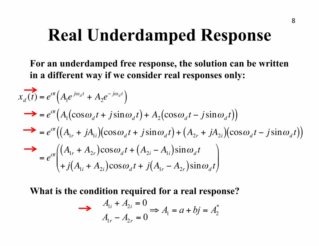
Real Underdamped Response 8

For an underdamped free response, the solution can be written in a different way if we consider real responses only:

What is the condition required for a real response?

€

xd (t) = eσt A1ejωd t + A2e

− jωd t( )= eσt A1 cosωd t + j sinωd t( ) + A2 cosωd t − j sinωd t( )( )= eσt A1r + jA1i( ) cosωd t + j sinωd t( ) + A2r + jA2i( ) cosωd t − j sinωd t( )( )

= eσtA1r + A2r( )cosωd t + A2i − A1i( )sinωd t

+ j A1i + A2i( )cosωd t + j A1r − A2r( )sinωd t

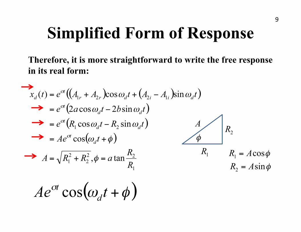
Simplified Form of Response 9

Therefore, it is more straightforward to write the free response in its real form:

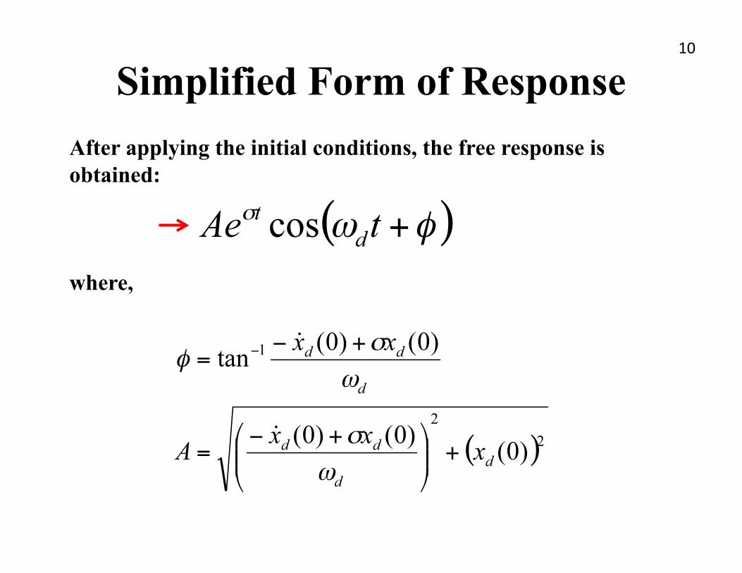
Simplified Form of Response 10

After applying the initial conditions, the free response is obtained:

where,

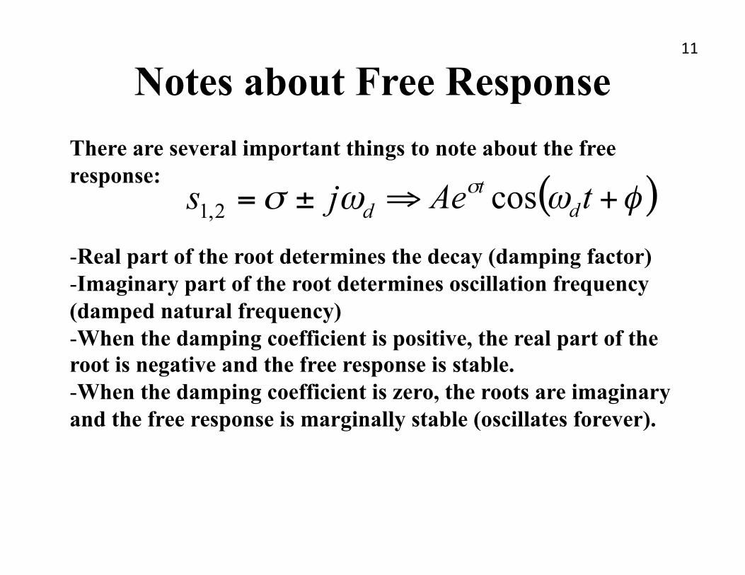
Notes about Free Response 11

There are several important things to note about the free response:

- Real part of the root determines the decay (damping factor) - Imaginary part of the root determines oscillation frequency (damped natural frequency) - When the damping coefficient is positive, the real part of the root is negative and the free response is stable. - When the damping coefficient is zero, the roots are imaginary and the free response is marginally stable (oscillates forever).

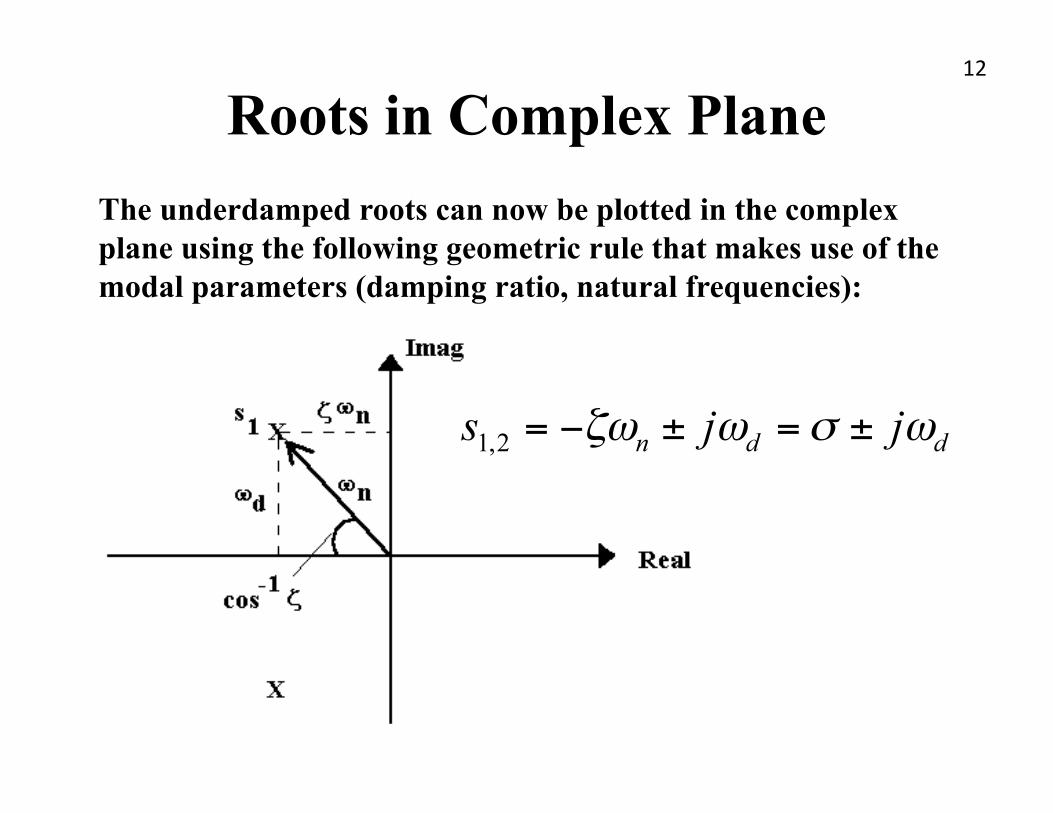
Roots in Complex Plane 12

The underdamped roots can now be plotted in the complex plane using the following geometric rule that makes use of the modal parameters (damping ratio, natural frequencies):

Visualizing the Free Response 13

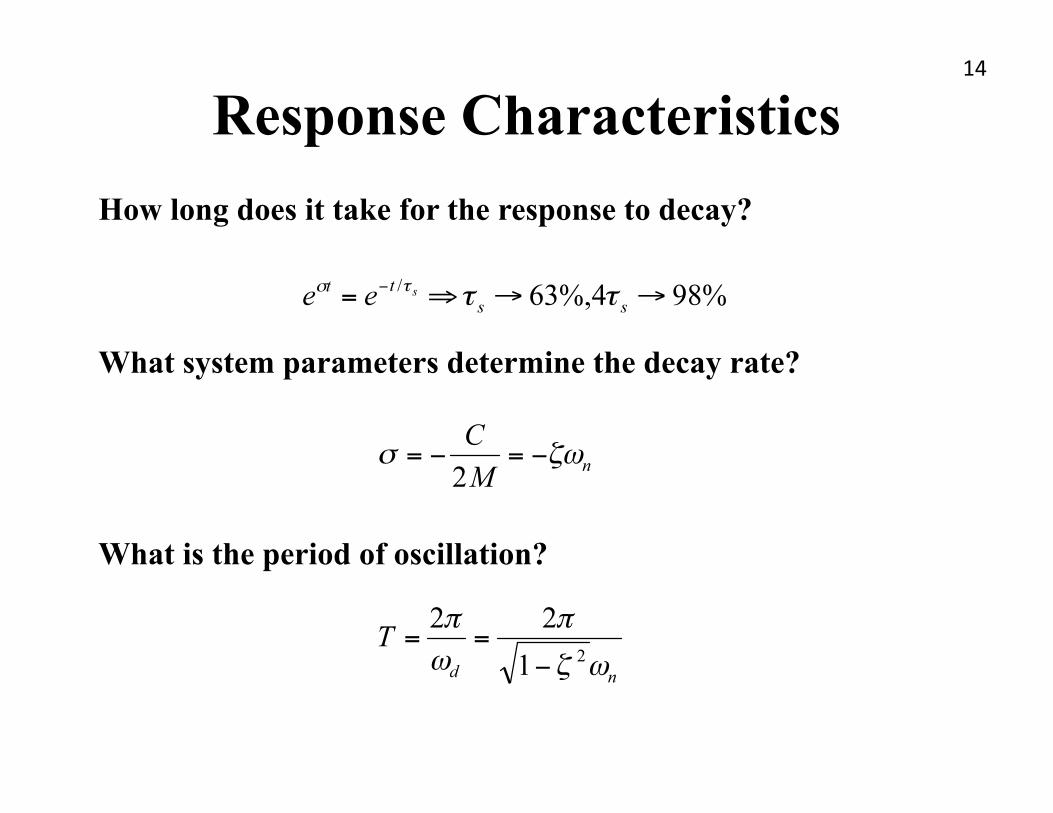
Response Characteristics 14

How long does it take for the response to decay?

What system parameters determine the decay rate?

What is the period of oscillation?

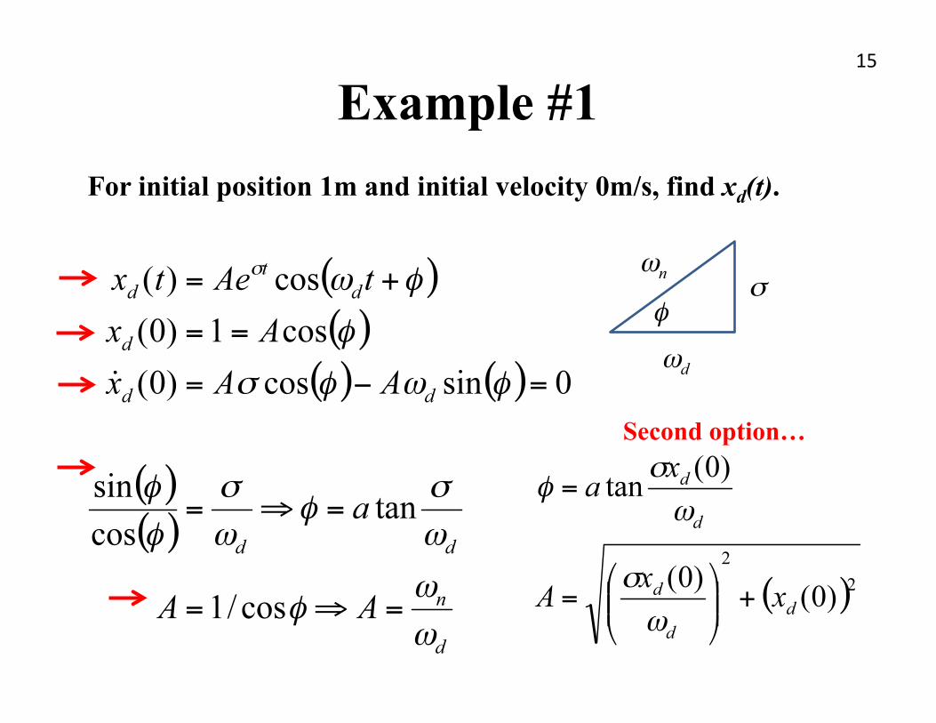
Example #1 15

For initial position 1m and initial velocity 0m/s, find xd(t).

Second option…

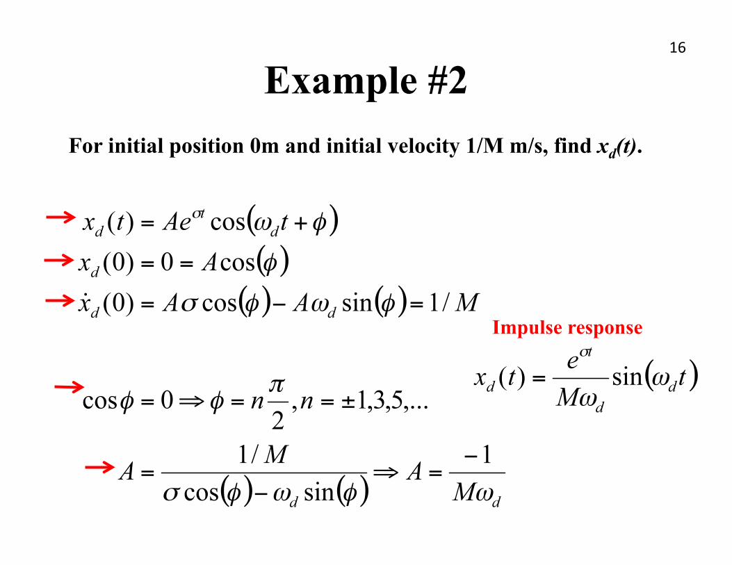
Example #2 16

For initial position 0m and initial velocity 1/M m/s, find xd(t).

Impulse response