ME 375 System Modeling and Analysis Section 9 – Block ... Handouts/chapter_9_bdcontrol.pdf · ME 375 System Modeling and Analysis Section 9 – Block Diagrams and Feedback Control

ME 375 System Modeling and Analysis

Section 9 – Block Diagrams and

Feedback Control

Spring 2009

School of Mechanical Engineering

Douglas E. Adams Associate Professor

G(s)

H(s)

-

Key Points to Remember

Block diagrams

Each block is completely independent of the block before and

after it (we assume there is NO LOADING)

Solve for the highest order term and then add blocks and

summing junctions until the equation is realized

Graphical description of algebraic Laplace relationships

Initial conditions are taken to be ZERO (particular solution)

Feedback control

If systems don’t respond the way we like, and if we can’t fix them,

we measure the response and correct for any error

Get there safely, fast, and do not oscillate/overshoot too much

We use feedback control to change the poles and zeros

We use feedback to stabilize, boost performance,

reject disturbances, and reduce sensitivity

© 2009 D. E. Adams ME 375 – Block diagrams and feedback control

9.1

Two Simple Examples First and second order systems

First order systems (e.g. low pass filter, sky-diver)

G(s)


9.2

Two Simple Examples First and second order systems

Second systems (e.g. SDOF system, LCR oscillator)

G(s) M


9.3

Input-output Block diagrams Decomposing G(s)

Sometimes we want to decompose G(s) into its

simplest components:

G(s) M

- -


9.4

Input-output Block diagrams Simplifying G(s) using Mason’s Rule and B.D. algebra

Sometimes we want to simplify combinations of

blocks into a single G(s) block:

- -

+

G(s)

H(s)

- = G(s)

1+H(s)G(s) Mason’s

Rule

+


9.5

Input-output Block diagrams Simplifying G(s) using Mason’s Rule and B.D. algebra

We can choose which simplifications we want to make

by combining certain blocks and pathways:

- -

+


9.6

Block diagrams for a DC motor Coupling between electrical, magnetic, and mechanical domains

How do we do this for coupled systems? (e.g., motor)

-

+

-

+

-

+


9.7

Example Vehicle speed control system

(demo)

-

+ + -

t

v(t) Increasing grade

Disturbance

Assumptions

Input/excitation

Output/response

S.S. error

Apply disturbance

Transient response

S.S. response

- Reduce response time - Reduce S.S. error

- etc.


9.8

Why Use Feedback Control? Getting from point A to point B in the right way

How do we get the system to respond the way we like?

A

B

G(s)

H(s)

-

+

Take system

from here…

Unstable

Too long

Too much

oscillation

Just right

To here

Stability

Speed

Accuracy

Forward T.F.

Feedback T.F. Open-loop T.F.

Closed

Loop T.F.


9.9

A Practical Example of Feedback Control Making the grade – How hard should we study?

CLOSED-LOOP T.F. (w/ grades)

-

+ Study time

Performance

Error Plant

Graders

Control law

What happens if

is large?

We get the grade

we wanted and it doesn’t

matter how hard the exam

is, in theory !

OPEN-LOOP T.F. (w/o grades)


9.10

Feedback Control and Block Diagrams S.S. error, disturbance rejection, sensitivity, and performance

In a servomechanism, we’d like to specify a position and

get there quickly and accurately:

- + + +

Plant

Steady state Disturbance

Sensitivity


9.11

Benefits of Feedback Control

Stabilizes unstable systems (HIGHEST PRIORITY!)

Reduces the effects of any disturbance

Reduces sensitivity to system parameters

In plant and control system

Enhances response characteristics

Speed of response (bandwidth)

Settling time

Percent overshoot

Reduces steady-state error

Regulation (keep it in one place)

Tracking (move it along a certain path)


9.12

Open-loop and Closed-loop Changing system behavior without changing the system

The system, or “plant”, may not respond the way we’d like

- -

+

Rl

Im

x

x

Poles

x

x

Poles we

want

How do we get to the poles?


9.13

Closed-loop System with Sensors and Actuators Getting to the poles…through feedback

The key to the poles is in the internal feedback loops

We get the new poles

by measuring the velocity and position,

and feeding that information back

- -

+

-


9.14

Feedback Control Vehicular speed control with unity feedback

OPEN-LOOP T.F.s

-

+ + -

CLOSED-LOOP T.F. (w/o disturbance)

Sensitivity

to M? S.S. error?


9.15

Feedback Control First order thermal environment control – an electric thermos

OPEN-LOOP T.F.s

-

+ +

Usually make these the same

R1 qi(t)

CLOSED-LOOP T.F.

Sensitivity

to Ta? S.S. error?


9.16

Feedback Control Servomechanism – speed control

By measuring the error, we can compensate for it!

- +

-

+

SPEED CONTROL


9.17

Feedback Control Servomechanism – speed control

-

+

OPEN-LOOP T.F.

CLOSED-LOOP T.F.


9.18

Feedback Control and the F.V. Theorem Servomechanism – speed control for step inputs

-

+

OPEN-LOOP T.F.

CLOSED-LOOP T.F. For large KP and Ko = Ki

Input speed


9.19

Fluid-Level Control Block diagram generation

wi

C1

R1

C2

R2

- +

-

+ +

Hoover Dam What if Rj goes to zero or infinity?


9.20

Fluid-level Control Block diagram reduction

- +

- + +


9.21

Fluid-level Control Block diagram (unity) feedback

OPEN-LOOP T.F.

Reference

level

Actual

level

Error signal

Actuation (control) signal

CLOSED-LOOP T.F.

-

+

Plant

Unity feedback


9.22

Steady-state Performance Servomechanism – Speed control vs. Position Control

-

+ TYPE 0

How can S.S. error go to zero?

-

+ TYPE 1


9.23

System Type – S.S. Error

Etc.

TYPE 0

Nonzero S.S. error

TYPE 1

Zero S.S. error

STEP

TYPE 1

Nonzero S.S. error

TYPE 2

Zero S.S. error

RAMP


9.24

Steady-state Error Changing the system type using the control law

-

+ +

CLOSED-LOOP T.F.s

R1 qi(t)

How do we get zero S.S. error?


9.25

Transient Performance Getting there quickly and in the “right” way

The plant responds according to the locations of its poles

- -

+

Im

Rl

x x

Poles

x

x

Poles we

want

1

Time [s]

y(t)


9.26

Transient performance Poles locations and transient response performance

The plant may not respond the way we’d like

- -

+

Rl

Im

x x x

x x x

x x

x

x

x

x

x

x

x


9.27

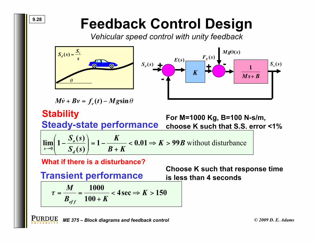
Feedback Control Design Vehicular speed control with unity feedback

-

+ + -

Transient performance Choose K such that response time

is less than 4 seconds

Steady-state performance Stability For M=1000 Kg, B=100 N-s/m,

choose K such that S.S. error <1%

What if there is a disturbance?


9.28

Feedback Control Design Servomechanism – Proportional speed control

- +

OPEN-LOOP C.E.

Open-loop

CLOSED-LOOP C.E.

Closed-loop

What if we want

to change the damping (simult.)?


9.29

Feedback Control Design Servomechanism – Proportional-derivative speed control

- +

CLOSED-LOOP C.E.

Closed-loop

Rl

Im

x x

x

x

x

x

O.L.

C.L. w/

KP

C.L. w/

KP,KD

Does this

Make sense?

What about the

S.S. error?


9.30

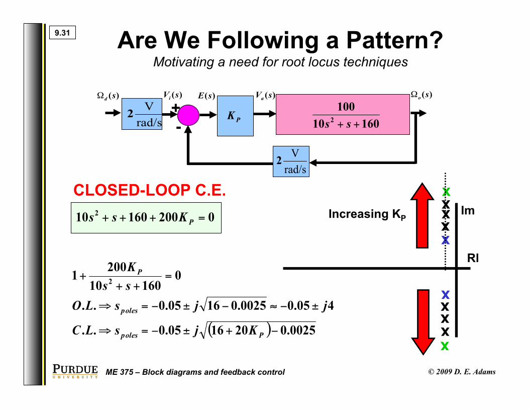
Are We Following a Pattern? Motivating a need for root locus techniques

- +

CLOSED-LOOP C.E.

x

Rl

Im

x

x

x

x x x

x x x

Increasing KP


9.31

- +

CLOSED-LOOP C.E.

Rl

Im

x x

x

x

O.L.

C.L. w/

KP,KD

x x x

x x x


9.32

Are We Following a Pattern? Motivating a need for root locus techniques

Root Locus Plotting the poles of the closed loop system

The characteristic equation changes when we close

the loop:

Rl

Im

-

+

X X

!

Gc (s)Gp (s)H(s) = "1

#Gc (s)Gp (s)H(s) = n180o

Gc (s)Gp (s)H(s) =1

Angle criterion

Magnitude criterion

OL poles

CL poles


9.33

Root Locus Rules for plotting root loci

Get the characteristic equation, in the following form:

Start at the OL poles, end at the OL zeros or infinity

# of paths = # of OL poles

Root loci are symmetric about the real axis and can’t cross

Root loci lie on the real axis to the left of an odd

number of real poles and/or zeros

Break away/in points are found

from dK/ds=0

Asymptotes go out at the angle

Rl

Im

X X OL poles

O


9.34

Root Locus Two poles with unity feedback and proportional control

Rl

Im

X X

symmetric

To left of 1 pole

Servo-position control

System The system never becomes

unstable even for infinite gain

-

+


9.35

Root Locus Two poles with proportional control and sensor dynamics

Rl

Im

X X X

symmetric

To left of 3 poles To left of 1 pole

OL poles pull the root loci to

the right (Why? Bode?) (I.e. they destabilize the CL system)

Servo-position control system with 1st order sensor dynamics

-

+


9.36

Root Locus Two poles with sensor dynamics and prop./deriv. control

Rl

Im

X X X O

symmetric

To left of 3 poles/zeros To left of 1 pole

End at OL zero

OL zeros pull the root loci

to the left (why? Bode?) (i.e. they stabilize the CL system)

-

+


9.37

Rl

Im

X X X O

symmetric

To left of 3 poles/zeros To left of 1 pole

End at OL zero

OL zeros pull the root loci

to the left (more this time---why?) (i.e. they stabilize the CL system)

-

+

Root Locus Two poles with sensor dynamics and prop./deriv. control


9.38

PID Control Steady-state and transient performance using PID

The plant may not respond the way we’d like

- +

Speed, freq.,

SS acc.

SS acc. (- phs.)

Trans./damping

(+ phs.)

- +

- +

- + +

Remember these?


9.39

Satellite Attitude Control A second order system with a double integrator

Rl

Im

X X

EOM

OLTF

Analysis: 1) What does the step

response look like? 2) What is the SS error?

3) Is this acceptable?

Plant poles

Control: 1) We want zero SS error in the step resp.

2) We want an overshoot of < 50% 3) We want a settling time of 10 sec


9.40

Satellite Attitude Control What about proportional control?

Rl

Im

X X

CLTF

CL poles

This isn’t good enough…we get zero SS error (w/o dist.),

but we can only choose the natural frequency – we don’t even have a damping ratio

1) Root loci are symm.

about the real axis 2) Loci approach OL zeros

or Infinity at angles of


9.41

Satellite Attitude Control What about proportional-derivative control?

Rl

Im CLTF

CL poles

1) ! Root loci lie on real axis

to left of odd # of OL poles/zeros 2) Root loci are symm.

about the real axis 3) Loci approach OL zeros

or Infinity at angles of

Can you find

this point?

What’s next?

X X O


9.42

Satellite Attitude Control Designing the control law

Rl

Im

CLTF

CL poles

X

X

What if we want to draw

the loci for varying KP?

X X O


9.43

Documents

ME 375 System Modeling and Analysis Section 9 – Block ... Handouts/chapter_9_bdcontrol.pdf · ME 375 System Modeling and Analysis Section 9 – Block Diagrams and Feedback Control