2 Multisource electromagnetic modeling using block Krylov ...upcommons.upc.edu/bitstream/handle/2117/85150/A...Multisource electromagnetic modeling using block Krylov subspace methods

Multisource electromagnetic modeling using block Krylov subspace methods

Vladimir Puzyrev1 and José María Cela1,2

1 Department of Computer Applications in Science and Engineering, Barcelona Supercomputing Center,

2 Polytechnic University of Catalonia.

SUMMARY

Practical applications of controlled-source electromagnetic modeling require solutions for

multiple sources at several frequencies, thus leading to a dramatic increase of the computational

cost. In this paper we present an approach using block Krylov subspace solvers that are iterative

methods especially designed for problems with multiple right-hand-sides. Their main advantage is

the shared subspace for approximate solutions, hence, these methods are expected to converge in

less iterations than the corresponding standard solver applied to each linear system. Block solvers

also share the same preconditioner, which is constructed only once. Simultaneously computed block

operations have better utilization of cache due to the less frequent access to the system matrix. In

this paper we implement two different block solvers for sparse matrices resulting from the finite-

difference and the finite-element discretizations, discuss the computational cost of the algorithms

and study their dependence on the number of right-hand sides given at once. The effectiveness of

the proposed methods is demonstrated on two electromagnetic survey scenarios, including a large

marine model. As the results of the simulations show, when a powerful preconditioning is employed,

block methods are faster than standard iterative techniques in terms of both iterations and time.

Keywords: Numerical modeling; Marine electromagnetic; Iterative solutions; Block methods.

1 INTRODUCTION

Electromagnetic (EM) methods have become established exploration tools in geophysics,

finding application in areas such as hydrocarbon and mineral exploration, reservoir monitoring, CO2

storage characterization, geothermal reservoir imaging and many others. Controlled-source

electromagnetic (CSEM) surveys in marine and land environments typically include tens or

hundreds of transmitters/receivers, while in airborne electromagnetics the number of sources in one

simulation experiment can reach thousands (Newman 2014). This poses serious challenges to

forward modeling and results in a high computational cost of 3D inversion.

In the context of CSEM multisource problems, special attention has been recently given to

Page 1 of 37 Geophysical Journal International

123456789101112131415161718192021222324252627282930313233343536373839404142434445464748495051525354555657585960

2 direct solvers based on Gaussian elimination (e.g. Streich 2009; Oldenburg et al. 2013). The most

computationally demanding part of these methods is the factorization, which involves only the

system matrix and thus needs to be performed just once. The solutions for different right-hand sides

(RHS) are then obtained only at the cost of two back substitutions each. The same factorization can

be also reused for symmetric matrices during the solution of the adjoint problem required by the

inversion algorithm (Schwarzbach & Haber 2013). Among the most popular direct solvers in

geophysics today one can mention a distributed-memory multifrontal MUMPS (Amestoy et al.

2006) and a shared-memory supernodal PARDISO (Schenk & Gartner 2004). However their huge

computational and memory requirements (which in 3D grow like O(N2) for time and O(N4/3

) for

memory, where N is the number of unknowns) impose severe limitations on the size of the problem.

Gutknecht (2007) reported a series of tests showing that direct solvers are competitive with the

iterative methods for two-dimensional problems, but not for three-dimensional ones. With the recent

progress in parallel direct solvers, these techniques have been successfully applied also for 3D

models, though their scalability is limited by relatively low computation-to-communication ratio

(Grayver et al. 2013).

Iterative methods, such as Krylov subspace solvers, are significantly less expensive in terms

of memory and computational time than direct methods. They typically require one or two matrix-

vector products and a few vector operations at each iteration, and hence can be efficiently

implemented on parallel computers. However, to be effective on real-world complex problems,

iterative solvers need a good preconditioner. Many of general-purpose preconditioners are fairly

robust and result in good convergence rates, but are highly sequential and difficult to implement

efficiently in parallel environments (Benzi & Tuma 1999). Several preconditioning schemes have

been developed or tuned for geophysical EM modeling purposes, including specific ones such as of

Weiss & Newman (2003) and general approaches like multigrid, both geometric (Mulder 2006) and

algebraic (Haber & Heldmann 2007; Koldan et al. 2014). In general, iterative solvers will be

efficient for large-scale 3D problems if 1) a good preconditioning scheme is applied; 2) multisource

problems are treated with some kind of reuse technique.

Several attempts have been made to combine direct and iterative methods. One of them is to

construct expensive ILU preconditioners and to re-use them for different source vectors (Um et al.

2013). Oldenburg et al. (2013) compared the performance of direct and iterative solvers for time-

domain EM problems, however due to the application of the preconditioner without re-use and quite

conservative drop tolerance value (10-10

), the iterative method performed poorly. Ren et al. (2014)

used a mixed direct/iterative solution approach for parallel finite-element method based on

nonoverlapping subdomains. More sophisticated solver techniques use Krylov subspace projection

as a model reduction technique for simultaneous solutions at multiple frequencies (hence, dealing

Page 2 of 37Geophysical Journal International

123456789101112131415161718192021222324252627282930313233343536373839404142434445464748495051525354555657585960

3 with multiple system matrices). The spectral Lanczos decomposition method and its extensions

(Druskin et al. 1999) can compute solutions for several frequencies at low cost which is, however,

sensitive to conductivity contrasts since convergence depends as a root of the fourth-order of the

condition number. Borner et al. (2008) developed a model reduction approach using rational Krylov

subspace projection. Zaslavsky et al. (2013) presented an inversion of large-scale 3D problems with

multiple sources and receivers with a forward solver based on the rational Krylov subspace

reduction algorithm with an optimal subspace selection allowing for a logarithmic convergence on

the condition number.

For the solution of a sequence of linear systems that have the same coefficient matrix, but

differ in right-hand sides, is often more efficient to use a special version of the solver instead of

applying the standard one to each of the systems individually. A group of methods called block

Krylov subspace solvers were successfully used in many areas of computational science and

engineering. Their two main benefits are much larger search spaces leading to a reduction in total

number of iterations and a use of block vector operations that can considerably reduce the number

of matrix accesses. For a detailed overview on block Krylov subspace methods we refer the reader

to Gutknecht (2007). During the last two decades, several different block solvers have been

developed and applied to many problems, ranging from electromagnetic scattering (Boyse & Seidl

1996) to acoustic full waveform inversion (Calandra et al. 2012).

In this paper we present efficient strategies for multisource EM modeling problems in

frequency domain using iterative block methods. We consider two underlying methods for spatial

discretization - the finite-difference electric-field method and the finite-element method based on

the reformulation in potentials, both briefly described in Section 2. The rest of the paper is

organized as follows. In Section 3 we review existing Krylov subspace solvers, introduce the block

QMR and block GMRES(m) methods and discuss preconditioning strategies. Both solvers have

been implemented in parallel and their scalability is compared to a direct method. Efficiency of the

block solvers for EM geophysical problems is demonstrated in Section 4. We examine convergence

behavior of the solvers, influence of the number of source vectors given at once, solver parameters

and different preconditioners on the performance. Finally, we draw some conclusions and point out

possible directions for further work in Section 5.

2 PROBLEM STATEMENT

Assuming harmonic time dependence i te

ω− , the diffusive Maxwell’s equations are:


123456789101112131415161718192021222324252627282930313233343536373839404142434445464748495051525354555657585960

4

0iωµ∇× =E H , σ∇× = +sH J E . (1)

Here E is the electric field, H is the magnetic field, 2 fω π= is the angular frequency and

sJ is an electric current source. The electric conductivity tensor σ varies in three dimensions,

while the magnetic permeability is assumed to be equal to the free space value 0µ . In the numerical

examples displacement currents are assumed to be negligible (since at low frequencies as σ ωε>> ),

though the codes support complex value iσ σ ωε= − I% and transverse electrical anisotropy. By

substituting H from the first equation of (1) into the second, we obtain the second-order electric

field equation

0 0i iωµ σ ωµ∇×∇× − = sE E J . (2)

The first method that we employ is based on a finite-difference (FD) discretization in the

frequency domain using staggered grids (Yee 1966). Until recently this was, perhaps, the most

popular approach for EM modeling in geophysics. It has been previously used for the simulations of

magnetotelluric (Mackie et al. 1994), CSEM (Newman & Alumbaugh 1995), and direct current

(Spitzer 1995) problems. The formulation is relatively simple and mesh building is straightforward.

Using the primary-secondary field formulation p s= +E E E , Eq. (2) reads

0 0 ( )s s p pi iωµ σ ωµ σ σ∇×∇× − = −E E E . (3)

After Eq. (3) is solved, the magnetic field is interpolated from the electric field values using

the Faraday’s law. From the computational point of view, it is important to note that finite-

difference discretizations on Cartesian grids produce banded or block-banded matrices. The code

can be easily organized in a matrix-free approach when no explicit storage of the matrix is required.

However, the simplicity of the FD discretizations comes with the well-known drawbacks of using

rectangular grids. The number of model parameters required to simulate realistic 3-D geologies can

exceed tens of millions (Commer & Newman 2008), hence using a direct solver becomes not

feasible. At low frequencies the convergence of iterative methods stagnates because of the null-

space arising from a curl–curl operator in (2) or (3). To avoid this, a scheme involving static

divergence correction (Smith 1996) or special preconditioning (Weiss & Newman 2003) can be

used.

For a large-scale multisource survey, using local grids for each source may be favorable

instead of one global grid (Commer & Newman 2008) since for structured grids the refinement

potential near the sources is very limited. A good 1D background model can be useful in this case

(Streich 2009), though, of course, it could not overcome all limitations of structured grids. In this


123456789101112131415161718192021222324252627282930313233343536373839404142434445464748495051525354555657585960

5 context, finite-element (FE) methods are considered as an alternative. The two main benefits of

unstructured meshes are their natural adaptivity to complex geometrical structures and large

reduction in the number of elements necessary to obtain a required accuracy of the solution. In the

context of multisource modeling, one mesh can be used for all sources. However, using

unstructured meshes is also a challenge, since robust adaptive mesh generation in 3D is still an open

question.

The second approach that we use here is the FE method based on a reformulation of Eq. (1)

in terms of gauged vector and scalar potentials, a common practice to solve EM problems in

geophysics (Everett et al. 2001; Weiss 2013; Ansari & Farquharson 2014). The following system

consisting of a vector and a scalar equation is to be solved:

20 0( ) ( )s s s p pi iωµ σ ωµ σ∇ + +∇Ψ = − ∆ +∇ΨA A A ,

0 0[ ( )] [ ( )]s s p pi iωµ σ ωµ σ∇⋅ +∇Ψ = −∇⋅ ∆ +∇ΨA A ; (4)

where the electromagnetic fields are connected to the magnetic vector and the electric scalar

potential as 10µ−= ∇×H A , ( )iω= +∇ΨE A . The implementation details are given in Puzyrev et

al. (2013). The discretization of Eqs. (3) or (4) with the FD or FE method leads to a large sparse

linear system of equations for each of the s source positions

k k⋅ =K x b . (5)

The RHS vectors kb 1,k s= contain information on the source current density. Boundary

conditions, typically Dirichlet, are embedded into matrix K , keeping it symmetric (but not

Hermitian). In structured rectangular grids each internal node has the same number of neighbors (6

for 3D) and hence banded matrices resulting from standard Yee discretizations have up to 13

nonzeros per row with complex entries located only on the main diagonal. Matrices resulting from

FE discretizations on unstructured tetrahedral meshes usually are several times denser since each

node is spatially linked to more neighbors.

Two completely different parallel codes are used in the numerical examples below. They are

based on Eqs. (3) and (4), respectively, and are referred to as FD and FE codes.

3 EFFICIENT SOLUTIONS STRATEGIES

In this section we discuss approaches to the iterative solution of the system (5), which is the

most computationally expensive part of the forward modeling. Before proceeding to the block


123456789101112131415161718192021222324252627282930313233343536373839404142434445464748495051525354555657585960

6 methods, we give a short overview of traditional Krylov solvers to better motivate our choice. Then

we discuss several preconditioners that were used with the block solvers to speed up the

convergence and make them more efficient in terms of computational time.

3.1 Krylov subspace methods

Krylov subspace solvers are a common choice for solving large sparse systems of linear

equations due to their low memory requirements and good scalability in parallel applications. A

total number of algorithms and their modifications is more than 100, however the number of

principal methods is one order of magnitude smaller. These methods differ in applicability, stability,

rate of convergence, memory and computational requirements. Since the fundamental operation that

dominates computing is the matrix-vector product (MVP), this number is crucial for determining

the cost of one iteration.

Due to historical reasons Krylov subspace methods are generally divided into two classes:

those for Hermitian matrices and those for general matrices. However, in computational

electromagnetics the matrix usually is symmetric but non-Hermitian, which makes impossible the

use of classical methods such as CG (Lanczos 1952), MINRES (Paige & Saunders 1975) or their

derivatives. Nevertheless, some algorithms can be applied at the cost of only one MVP per iteration.

Based on Arnoldi's process the generalized minimal residual (GMRES) method by Saad & Schultz

(1986) is one of the most popular and well-studied solvers suitable for non-symmetric and non-

Hermitian indefinite systems. Another important group of Krylov subspace solvers is based on the

Lanczos biorthogonalization procedure. These methods include the biconjugate gradient (BiCG,

Lanczos 1952; Fletcher 1975), its modification, the biconjugate gradient stabilized (BiCGStab, van

der Vorst 1992) and the quasi-minimal residual (QMR, Freund & Nachtigal 1991) among others.

For symmetric systems, the crucial point in terms of computational efficiency is that some of these

general non-Hermitian solvers can take advantage of the matrix symmetry. Indeed, QMR and BiCG

applied for symmetric problems involve only one MVP per iteration versus two for the general

versions and hence perform faster, though their stability and rate of convergence are often worse

than those of BiCGStab. The latter possesses many attractive properties and in the years following

the original publication was generalized to BiCGStab2 and BiCGStab(l), also appeared a variant

based on multiple Lanczos starting vectors called ML(k)BiCGSTAB. Finally, we should mention

the recently developed IDR(p) method (Sonneveld & van Gijzen 2008), which is based on the

induced dimension reduction theorem proposed in 1980 and not used as a solver for almost 30 years.

After the second attempt, the method attracted considerable attention since published studies


123456789101112131415161718192021222324252627282930313233343536373839404142434445464748495051525354555657585960

7 showed the fast convergence of IDR(p) for the values p>1. The convergence of BiCGStab and IDR

is often better than the one of the above-mentioned symmetric solvers, however they always require

at least 2 MVPs, which is impractical for symmetric matrices.

Fig. 1 illustrates the typical convergence scenario for three methods that require only one

MVP per iteration: GMRES with three different restart parameters, symmetric BiCG and symmetric

QMR. The system originates from a land CSEM scenario described in Section 4. We use

preconditioners of three different quality levels (presented in more detail below) to show the

differences in the solvers' behavior. First one (Jacobi) is “cheap” implying that the cost of each

iteration is very low, second one is “mediocre” (ILU with drop tolerance 10-4

), and the third one is

“good” (ILU with drop tolerance 10-6

). With a cheap preconditioner (Fig. 1a) the convergence is

slow, residual norms of GMRES decrease monotonically, though QMR and BiCG typically have a

similar rate of convergence (the latter has rapid oscillations in the error norm). Alumbaugh et al.

(1996) compared BiCG and QMR methods and chose the former because of its more stable nature.

When the preconditioner is “mediocre” (Fig. 1b), QMR fails to converge, while GMRES

(expectedly) and BiCG (quite surprisingly) perform well. When the preconditioner is sufficiently

good, all methods perform reliably (Fig. 1c). All variants of GMRES again converge slightly faster

in terms of iterations and computational time.

3.2 Block solvers

A straightforward approach to CSEM forward modeling using iterative methods is to solve

each system separately with parallelization over sources and frequencies, but without parallelization

of the solver (e.g. Plessix et al. 2007). This results in a very small cost of communications since

only problem data and the resulting solution need to be distributed among the computational nodes.

However, the overhead for a multisource problem is quite large since this approach presumes

independent initialization, construction of the preconditioner and storage of multiple copies of

matrices and vectors for each source. Large-scale, massively parallel schemes typically use a

domain decomposition paradigm and parallelize solver (Alumbaugh et al. 1996). The achieved

speedup slowly degrades with increasing number of cores, because of the overhead due to message

passing. The preconditioner for iterative methods, as well as LU factorization for direct ones, can be

constructed only once and then re-used for different RHS (Um et al. 2013).

Instead of solving each of the systems with independent Krylov iterations, it is often more

efficient to use a block version of an iterative solver. A block Krylov subspace method for solving a

linear system with s RHS vectors generates approximate solutions mx such that


123456789101112131415161718192021222324252627282930313233343536373839404142434445464748495051525354555657585960

8

0 0( , )m m− ∈x x B K r� ; (6)

where 0( , )mB K r�

is a block Krylov subspace defined as

1

0 00

( , ) ;m

j s s n sm j j

j

γ γ−

× ×

=

= ∈ ∈ ∑B K r K r C C� ; (7)

and 0 0, n s×∈r x C are the initial block residual and guess, respectively. It is important to note that

jγ are not scalars (as in the case of the global methods), but s s× matrices. In this way, each of the

s columns of 0m −x x is approximated by a linear combination of all the s m× columns in the

sequence 1

0 0 0, , m−r Kr K rK . For a more detailed overview of mathematical foundations we refer

the reader to Gutknecht (2007).

Similar to the standard Krylov solvers, the optimal solution is computed in an iterative

manner. The main advantage of block methods is that the searching subspace for approximate

solutions is the sum of all single Krylov subspaces. Hence, block solvers are expected to converge

in less iterations than the corresponding standard method applied to each linear system. Possible

linear dependence of residuals opens perspectives for a larger speedup, but makes an

implementation more challenging. The two main drawbacks are larger memory requirements and

additional operations during each iteration to maintain stability of the block method. The latter

requires that either the system matrix is relatively dense or powerful preconditioners are used to

make the block solvers more efficient than the standard ones.

Most of the standard Krylov subspace solvers have a block variant, however they differ a lot

in stability and degree of investigation. Based on the discussion in the previous subsection, we

choose two different Krylov methods to implement their block version: GMRES and QMR. Block

variants of both methods exist and are well-studied, especially the first one. The block GMRES

(BGMRES) method has been developed for over two decades; recent contributions include Baker et

al. (2006) and Calandra et al. (2012). As a natural extension of the GMRES method, it is based on

the block Arnoldi process and uses a standard block-wise construction of the basis vectors. The

original method requires the computation and storage of an orthogonal basis, making memory and

computational cost unacceptable for a large number of iterations, so restarted or truncated versions

are applied in practice. The computational efficiency of BGMRES is influenced by the relation

between the restart parameter m and the number of RHS vectors s. The method is given in the

Appendix.

The second method is the block QMR (BQMR) introduced by Freund & Malhotra (1997).


123456789101112131415161718192021222324252627282930313233343536373839404142434445464748495051525354555657585960

9 For complex symmetric or Hermitian matrices the classical Lanczos process simplifies, resulting in

one sequence of Lanczos vectors instead of two for the general case. For the implementation, we

choose the version of Malhotra et al. (1997), which, like the symmetric QMR method, exploits the

matrix symmetry and thus requires twice less expensive MVPs. The basis vectors in this block

method are constructed in a vector-wise approach. Another variant of BQMR for complex

symmetric systems is the one of Boyse & Seidl (1996); the differences between these two

approaches are discussed in Freund & Malhotra (1997). The structure of the BQMR algorithm is

more complicated than of the BGMRES; for implementation details we refer the reader to

Algorithm 4.1 of Malhotra et al. (1997) and to the discussion in this and other papers and technical

reports by the authors.

A lot of sources (e.g. Gutknecht 2007; Du et al. 2011; Calandra et al. 2012) compare the

computational cost and memory requirements of block methods and solving each system separately.

The number of expensive operations with the system matrix per iteration is always the same (we

recall that the block methods are expected to converge in less iterations), while for the number of

vector updates α= +y x y the ratio between block and non-block methods is O(s). Memory

requirements of block solvers are also about s times larger, however, this estimate is excluding

storage of the coefficient matrix and preconditioner, which are stored only in one instance of the

solver. In the numerical examples below, we show the performance counted by both MVPs and

computational time. The scheme can be summarized as follows:

1) One mesh which includes all or a subset of the sources is used for the discretization. A

block solver has access to the system matrix and all RHS vectors.

2) An expensive preconditioner is created once at the beginning and used in the whole

iterative process.

3) A block solver is expected to be computationally more efficient than standard techniques

since:

a) Much larger subspaces lead to a significant reduction in terms of iterations required

for the convergence. Hence, the number of MVPs and preconditioner applications is

smaller compared to the non-block methods.

b) Simultaneously computed block vector operations have better utilization of cache

due to the less frequent access to the stored matrix or less “on the fly” computations

in the matrix-free implementations (e.g. Weiss 2013 and other papers by the author).

For a block-wise method, this optimization is straightforward. For BQMR, which is

originally a vector-wise method, MVP implementation in a block manner is also

possible (see Freund & Malhotra 1997), however, is more complicated.

c) A block method can include a deflation – procedure to detect and remove linearly or


123456789101112131415161718192021222324252627282930313233343536373839404142434445464748495051525354555657585960

10

near-linearly dependent vectors in block Krylov subspaces. It is possible at the

beginning (the so-called initial deflation) or during the iterative process. Clearly,

deflation leads to a further reduction of MVPs needed to solve the problem.

Before proceeding further, we should note that there are two alternatives to block methods.

The first one is the so-called seed methods (see Simoncini & Gallopoulos 1995 or Gutknecht 2007

and references therein) when a single system is chosen as a seed system, a corresponding Krylov

subspace is obtained and thereafter initial residuals of all the other systems are projected to this

subspace. These techniques can be useful in the case when not all right-hand sides are available at

the same time. The second alternative is the so-called global methods (Jbilou et al. 1999), which use

a global projection onto a matrix Krylov subspace. However, both these techniques have received

less attention than block methods.

3.3 Preconditioning

It is well-known that the successful use of iterative solvers depends on preconditioning.

There are several reasons that cause convergence to stagnate, including large aspect ratios of the

elements in the model, large conductivity contrasts, low frequencies or presence of a large air layer

(the latter two directly affect the second term of Eq. (3)). A good preconditioner can make an initial

ill-conditioned system converge quite rapidly. We consider below several preconditioning schemes

to be used together with the block methods. For testing purposes, we also use a standard diagonal

(Jacobi) preconditioner, which is effective to some extent for diagonally dominant matrices.

However, the key idea is to use an expensive preconditioner which, after being computed for a

given frequency, is used in one or several block solver instances with all source vectors.

Incomplete LU (ILU) preconditioners (Saad 2003) are among the most reliable and widely

used techniques. They are based on a factorization of the original matrix into a product of a lower

triangular matrix L and an upper triangular matrix U. In general, as the fill-in level of an ILU

decomposition increases, the quality of the preconditioner improves, however with an increased

cost of the factorization and forward-backward solves. Various ILU techniques differ in strategies to

prevent an excessive fill-in. For example, ILUT uses a threshold when deleting small but nonzero

elements. For a symmetric indefinite matrix an LDLT factorization algorithm with pivoting (Golub

& Van Loan 1996) can be applied. Indeed, if a symmetric matrix T=A A can be factored as

T T= =A LDU U DL where D is a diagonal matrix, then T=U L and T=A LDL . Thus, the

memory demand for storing the preconditioner is halved and the computational time is reduced.

Being closely related to the direct methods, ILU preconditioners share the same drawbacks.


123456789101112131415161718192021222324252627282930313233343536373839404142434445464748495051525354555657585960

11 They are feasible only when the matrix size is not prohibitively large and are not naturally suitable

for parallel implementation. During the last decade several approaches for ILU parallelization have

been published, however they still remain difficult to implement and lead to a degradation of

performance on massively parallel machines. On the contrary, another group of methods,

approximate inverse preconditioners, are well suited for a parallel implementation, but often lack

robustness. For example, the performance of several tested approximate inverse preconditioners

with static and dynamic sparsity pattern strategies for the systems resulting from the FD

discretization was unsatisfactory in some cases. However, for the formulation in potentials, the

truncated approximate inverse (TAI) preconditioner from Puzyrev et al. (2013) and its variants

based on topological and geometric approaches for an a priori chosen sparsity pattern performed

reliably. Hence, we use this preconditioner with the block methods in the FE code.

One of the most powerful groups of preconditioners are multigrid methods. In contrast to

any one-level preconditioner, multigrid techniques reduce all error components, both short and long

range. We have implemented a simplified geometric multigrid (MG3) preconditioner that is used in

the tests with the FD scheme. Due to implementation restrictions, the number of inner levels is

limited to 3. Based on a series of experiments, as a smoother we choose three iterations of a damped

Jacobi with the damping parameter 0.4ω = . Undamped version of the smoother ( 1ω = ) proved to

be very unreliable. Another possible choice is Gauss-Seidel, which is a quite powerful smoother and

is highly parallel when the red-black ordering scheme is used (Trottenberg et al. 2001). For our

purposes to show the efficiency of the block Krylov subspace methods with a robust reusable

preconditioner, ILU, TAI or MG3 are a good choice. None of them is flawless, however

development of an optimal parallel preconditioner is outside of the scope of this paper. We do not

consider here variable preconditioners that can be modified during the solution process, though they

also can be used together with a flexible variant of a BGMRES.

Scalable performance of a linear solver is important in order to efficiently exploit modern

computational systems. As it was pointed out in the introduction, the scalability of direct methods is

usually quite low and limited by implementation of the multifrontal method, while iterative methods

strongly depend on the preconditioner. Fig. 2 shows the scalability in strong sense (increasing

number of subdomains for a fixed problem size) of an iterative method with the above-mentioned

preconditioners versus the MUMPS direct solver. As expected, the simple preconditioning

techniques scale better than the more sophisticated ones, while the direct solver reaches its

scalability limit at 32 MPI ranks.

Iterative solutions can be accelerated further using initial guess obtained from the previous

results. To overcome the effect of rapid attenuation of the EM field in conductive media, we use an

interpolation of the resulting solution from the previous source. This does not affect the solution


123456789101112131415161718192021222324252627282930313233343536373839404142434445464748495051525354555657585960

12 accuracy, but can make an iterative process converge faster. Newman & Alumbaugh (1995) used the

previous solution and reported about a 10-15% reduction in the CPU time compared with a zero

initial guess. The efficiency depends on the problem, for example, for complex models (e.g. with

non-flat bathymetry) the gain would be smaller or non-existent. Um et al. (2013) reported

inefficiency of their initial guess approach (called solution bootstrapping) for one of their models,

while for another one it resulted in a 10% gain. For the marine CSEM model described below we

obtained a 5% speedup using the previous solution without interpolation and up to 10% using cubic

interpolation. For problems that are 1D or 2D in nature, the maximum gain was about 15% of

computational time. We cannot expect a better approximation to the solution since it is limited by

numerical errors of the second-order FD scheme.

4 NUMERICAL EXAMPLES

In this section we illustrate our approach using two 3D examples. The first one describes a

land scenario with simplified targets and is used to test the solvers for a non-complex case and to

study their convergence behavior. In the second example, we aim to demonstrate the efficiency

from an application point of view on a real-size complex model in marine environment. Both FD

and FE methods are used for forward modeling.

4.1 Two-anomaly CSEM model

As a first model, we consider a homogeneous 12 x 10 x 4 km half-space containing two

anomalies (Fig. 3). A large conductive (1 S/m) box is located at the left part at a depth of 0.7 km,

while a thin resistive (0.02 S/m) body is in the right part at a depth of 0.3 km. An air layer at the top

of the model results in a huge conductivity contrast between 0.1 S/m half-space and 10−8

S/m air. 20

sources are placed on the surface at 1.2 km spacing. This simple model can be easily discretized

with the FD method resulting in ~1.2 million of unknown electric-field values for the frequency of

5 Hz. The discretization with the FE tetrahedral elements produces about 0.4 million of unknowns.

Since these systems are quite small, the simulations were performed on a desktop Intel i7 machine

with two @2.8GHz cores. Both methods have shown a good agreement in the results, for example,

the amplitudes and phases of the Ex field component are compared in Fig. 4 (a, b). The relative error

at the receivers between these two codes stays within 1% in amplitude and 1° in phase. Fig. 4 (c)


123456789101112131415161718192021222324252627282930313233343536373839404142434445464748495051525354555657585960

13 illustrates the ratio between the Ex amplitudes in the central part of the modeling domain, the

maximum error is less than 2%. Expectedly, the FE method requires nearly two thirds fewer

unknowns than the FD approach. Some discrepancies in the regions with highly varying

conductivity are related to the numerical differentiation of the solution of Eqs. (4) in the FE code.

Next, we compare the performance of block solvers versus standard ones. Note that BQMR

and BGMRES work with the vectors in a vector-wise and a block-wise manner, respectively. This

means that one iteration of BQMR includes one individual MVP, while one BGMRES iteration has

a multiplication of the matrix by the block of s vectors. To avoid any misinterpretation, we give the

number of MVPs instead of the number of iterations. Each block MVP is counted as s MVPs

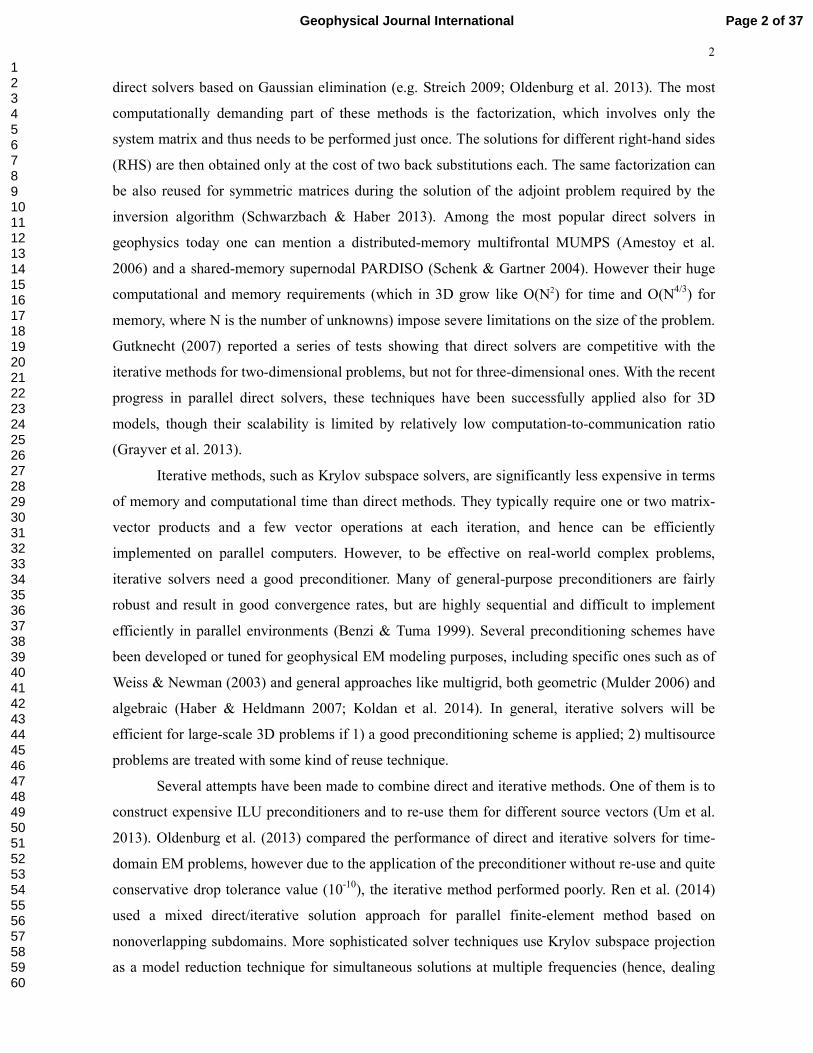
though it is performed even faster due to cache effect. Fig. 5 shows the histories of the relative

residual norms of BQMR and QMR, both preconditioned by the simple Jacobi method. This is a

typical convergence behavior for block versus non-block solvers. BQMR saves about one-third of

the MVPs required to converge. However, these results look promising only until we look at the

corresponding CPU time. Indeed, in terms of the computational time BQMR (s = 10) actually

performed worse than 10 calls to QMR: 1045 seconds versus 878 (FD code). The reason is that,

since the system matrix preconditioned by the Jacobi method is very sparse, the computational cost

of the MVPs is comparable to the other operations of the algorithm, such as dense vector operations.

Clearly, in this case the computational overburden from the additional operations of block methods

required to maintain block stability (not considered in Fig. 5) negates any gain. We recall that block

methods perform faster than standard ones under the condition of relatively expensive matrix

operations. For complex real-world problems, the use of efficient and expensive preconditioners is

mandatory, and this is precisely the case where block algorithms perform superior to conventional

methods.

In Table 1 we present the computational cost of the finite-difference simulations when

expensive preconditioners, namely ILU and MG3, are employed. When choosing drop tolerance for

ILU, the tradeoff in performance is between reducing the number of iterations required to converge

and increasing the cost of each iteration and preconditioner construction. Here we choose the value

10–5

in order not to make the memory requirements too large. From Table 1 we can make the

following observations. First, the use of expensive preconditioners significantly reduces CPU time

and makes block methods preferable, since the preconditioning and MVPs dominate the

computation. For all cases considered, the block solvers required fewer MVPs and preconditioner

applications than the standard methods. Second, with the increasing number of RHS vectors, the

average number of MVPs per source for both block solvers is monotonically decreasing. Third, the

number of MVPs is nearly the same for BGMRES(5) and BQMR. The latter performed a bit worse

with the ILU preconditioner and competitively with the MG3, except the case s = 20 when


123456789101112131415161718192021222324252627282930313233343536373839404142434445464748495051525354555657585960

14 convergence stagnated. Also, when a less accurate ILU preconditioner with the drop tolerance of

10–4

was used, BQMR was not able to converge. In general, with a good preconditioning the block

solvers perform more efficiently in terms of computational time than standard solvers applied to the

linear systems one by one. On average, the speedup for s = 20 is ~1.8x and ~1.55x for ILU and

MG3, respectively. When making the comparisons, we assumed that the preconditioners are

computed only once and then are shared between all solvers, which is the proper way to do.

4.2 Complex marine CSEM model

In this section we demonstrate how the block solvers can be applied to large modeling

problems when we have quite limited computational resources at our disposal, say, a part of a

cluster. Actual simulations were performed on 32 nodes each having two 8-core Intel Xeon E5-2670

@2.6 GHz processors and 32 GB of memory. The synthetic model shown in Fig. 6 represents a

marine CSEM scenario. The receivers are located at 0.7 km spacing along 8 lines on a moderate

bathymetric relief ranging from 1.0 to 1.2 km. 120 positions in total were considered in the

simulations. The transmitter is a horizontal electric dipole towed 30 m above the receivers. The

conductivity of the seabed is considered anisotropic and varies from 1.4 to 0.02 S/m. The sea water

conductivities are in the range 3.2–3.3 S/m, the air layer is set to 10-6

S/m. At the depth of 800–

820 m below the seafloor the target thin resistive (0.021–0.018 S/m) body is located.

At 2 Hz frequency, the smallest skin depth in the sediments is around 300 m. For the FD

simulations we choose the grid spacing to fulfill a requirement of 4 points per skin depth. Outside of

the central region the cells are stretched in x and y. Spacing in z direction is 20 m near the seabed

and slowly increasing with the depth. The final dimensions of the grid are 162 x 148 x 140,

resulting in ~10 millions of complex unknowns. This poses a significant challenge in terms of

memory for direct solvers since even a total amount of 1 terabyte will be not sufficient. With the FE

method we aim at much better spatial discretization and create a mesh with various local

refinements in the areas of interest. This system has ~5.5 millions of unknowns. TAI and MG3 were

used as right preconditioning for the FE and FD methods, respectively. The stopping tolerance for

all solvers was set to 10−6

.

The forward modeling results displayed in Fig. 7 as a ratio between the responses for the

model with the thin resistor and without it shows that the target is detectable with the current

configuration. The computational cost of the FE simulations for the different number of RHS is

presented in Fig. 8. Again, when block methods with a non-trivial preconditioning are employed,

both the iterations (Fig. 8a) and computational time (Fig. 8b) are saved. As for all block methods,


123456789101112131415161718192021222324252627282930313233343536373839404142434445464748495051525354555657585960

15 the cost of one BQMR or BGMRES iteration increases with the number of RHS, while the number

of MVPs per RHS decreases. For example, with an increase in s from 5 to 40, this number reduces

from 114.3 to 65 for BGMRES+ILU. The non-block solver (s = 1) required, on average, 146.7

MVPs and preconditioner applications per source. As can be seen from Fig. 8b, BGMRES saves

almost half of the CPU time for this model. The performance of BQMR is similar, however it

deteriorates faster with an increasing s. The best performance is achieved for BGMRES with s = 40

and s = 60 (all 120 sources are given in three and two portions, respectively). For a larger number of

RHS vectors and a relatively weak preconditioner, the iterative block solution becomes unreliable.

Fig. 9 shows the number of MVPs and CPU time for the simulations with the FD code using

ILU and MG3 preconditioners. Again, the largest savings in terms of computational time were

obtained with the BGMRES solver. The optimal value of s for this model discretized with either FD

or FE methods is around 40–60 leading to a twofold speedup. When the number of RHS given at

once exceeds 20–40, BQMR starts experiencing problems with convergence, while BGMRES still

performs well provided the preconditioners are robust enough. Also, the relative role of the

additional block operations becomes more dominant with an increase in s, which explains the larger

computational times despite the smaller number of MVPs and preconditioner applications. This is

similar to the results of applying block methods to the other problems (Du et al. 2011; Calandra et al.

2012).

Storage cost of the sparse matrices, TAI and MG3 preconditioners was comparably low (10–

20 Gb), while the ILU barely fitted into 0.5 Tb of memory even with the symmetry accounted for.

Memory requirements for the temporal block vectors are approximately s times larger than needed

for one source with a non-block solver. In the worst case (BGMRES(5) with s = 60 for the FD

model) this cost was around 70 Gb. However, it is still much smaller than a direct method would

require for a problem of this size. Also, s instances of a non-block solver running independently on

s computing cores would require more memory since the matrix and the preconditioner are stored in

each local instance. The growth of the memory requirements with respect to the number of degrees

of freedom is linear for the most expensive parts of the solver (except the preconditioner). For

example, a structured grid for the 2.5 Hz frequency and the same number of points per skin depth

results in ~40% more unknowns in the system. The total storage cost for BGMRES(5) with s = 60

and MG3 preconditioner was around 140 Gb for this case against 90 Gb for the 2 Hz system.

Finally, we have tested the impact of the GMRES restart parameter m on convergence rate

and CPU time. Fig. 10 shows the number of MVPs and corresponding time of BGMRES(m) with m

ranging from 5 to 15. Similar to the non-block GMRES method, with the larger values of the restart

parameter the method needs fewer MVPs to converge. Optimal in terms of computational time

values of m depend on complexity of the preconditioner, however the changes are quite small. For


123456789101112131415161718192021222324252627282930313233343536373839404142434445464748495051525354555657585960

16 the BGMRES(m)+ILU combination, the optimal values of the restart parameter are 10…12. A

slightly cheaper MG3 preconditioner shows the best performance for m = 8…10, while for the larger

values of m the gain in convergence is suppressed by the more costly Arnoldi loop. In Fig. 11 we

show the performance of GMRES(10) and BGMRES(10) as an average number of MVPs and CPU

time per source. Here we also use the interpolation from the previous solutions as an initial guess

for the block method. The convergence rate of standard GMRES is independent of the number of

RHS, while the block solver performs approximately two times faster applied to several tens of the

sources simultaneously.

5 CONCLUSIONS AND OUTLOOK

Forward modeling problems for multiple sources operating at a common frequency result in

a sequence of linear systems with the same coefficient matrix and different right-hand sides. This

situation is beneficial for modern parallel direct solvers that are becoming increasingly popular also

for 3D problems. Most likely, these methods will be successfully used by the geophysical

community in the future for medium-scale finite-element discretizations, where the geometric

complexity of the problems can be handled by using unstructured meshes and resulting matrix is not

very large and more dense. However, beyond a certain problem size, use of direct solvers becomes

too expensive. Due to the nonlinear growth of their computational and memory requirements, a

moderate increase in the size of a model will require a large growth of the computing facilities.

We have implemented and tested two iterative solvers based on block Krylov techniques.

These methods, which have found application in many other problems, are also suitable for the

simulation of the EM phenomena in geophysics. Like traditional Krylov solvers, they do not have

strict computational and memory limitations on the problem size, express a high level of

parallelization and, thus, can be applied for large-scale multisource problems when the size of the

coefficient matrix does not allow an efficient use of a direct solver. Main computational benefits

over non-block techniques include potentially smaller number of iterations required for convergence,

simultaneously performed block matrix-vector operations and an explicit reduction of the block size,

called deflation. Block Krylov methods are advantageous when the cost of matrix-vectors

operations is high compared to other operations, like in the case of dense matrices. However, this is

not the case even for geometrically complex problems discretized with the FE methods, and

moreover for the traditional FD methods that use structured grids and yield very large banded (but

not Toeplitz) and extremely sparse matrices. Thus, a powerful preconditioning technique should be

used together with the block methods. We have tested three different preconditioners and received


123456789101112131415161718192021222324252627282930313233343536373839404142434445464748495051525354555657585960

17 up to a 2x speedup over solving multiple systems individually.

Based on our numerical experiments, we conclude that the BGMRES method performed

more reliable and stable in most of the cases. BQMR solver has also shown savings in MVPs and

computational time over solving each system separately, however its convergence begins to stagnate

when the number of RHS vectors is relatively large. Also, the structure of the latter algorithm is

more complicated and its implementation on parallel machines encounters more difficulties than the

one of BGMRES. In general, the implementation of non-block Krylov solvers is much less

challenging than of block ones that support deflation. However, these methods have received

growing attention during the last years and they are likely to be included in the popular linear

algebra packages. At the present time, several versions of BGMRES are present in the Belos

package of the Trilinos software collection (Bavier et al. 2012). To make possible the use of block

methods, the model grid must be the same for a group of sources. This is similar to the use of direct

solvers when any grid adaptation would require a new factorization. Block solvers can be a golden

mean between using local meshes (one per source position) and global meshes (one for the whole

domain). We suggest using BGMRES (or related Krylov methods) for the sub-problems that include

several tens of the sources. By varying the number of source vectors, solver parameters such as

restart parameter m, and preconditioner, it is possible to better adapt the problem to different

computing environments.

Another possible use of block methods is the solution of the inverse problem when the

computation of the full Jacobian is required. If both sources and receivers can be combined together

in a block right hand side, the accuracy of the computations at the receiver is squared, and thus the

algorithm requires less iterations to converge. This approach can potentially lead to another speedup

by a factor of 2.

Methods based on Krylov subspaces are not limited to a sequence of linear systems with

identical matrix, but can also handle similar matrices. Parks et al. (2006) have presented an

overview of Krylov subspace recycling techniques for sequences of linear systems, where both the

matrix and the RHS change. When a source frequency or a conductivity of some region is changed,

rather than discarding the vector space generated from a previous solution, these methods can re-use

it to reduce the total number of iterations.

ACKNOWLEDGMENTS

Funding for this work was provided by the Repsol-BSC Research Center and the RISE

Horizon 2020 European Project GEAGAM (644602). MareNostrum Supercomputer was used for


123456789101112131415161718192021222324252627282930313233343536373839404142434445464748495051525354555657585960

18 the numerical tests. The authors express their thanks to Rene-Edouard Plessix, Mikhail Zaslavsky

and one anonymous reviewer for their valuable comments that significantly helped to improve the

paper.

REFERENCES

1. Alumbaugh, D.L., Newman, G.A., Prevost, L. & Shadid, J.N., 1996. Three-dimensional

wideband electromagnetic modeling on massively parallel computers, Radio Sci., 31, 1–23.

2. Amestoy, P.R., Guermouche, A., L'Excellent, J.Y. & Pralet, S., 2006. Hybrid scheduling for the

parallel solution of linear systems, Parall. Comput., 32(2), 136–156.

3. Ansari, S. & Farquharson, C., 2014. Three-dimensional finite-element forward modeling of

electromagnetic data using vector and scalar potentials and unstructured grids, Geophysics, 79,

1–17.

4. Baker, A.H., Dennis, J.M. & Jessup, E.R., 2006. On improving linear solver performance: A

block variant of GMRES, SIAM J. Sci. Comput., 27, 1608–1626.

5. Bavier, E., Hoemmen, M., Rajamanickam, S. & Thornquist, H., 2012. Amesos2 and Belos:

Direct and iterative solvers for large sparse linear systems, Sci. Program., 20(3), 241–255.

6. Benzi, M. & Tuma, M., 1999. A comparative study of sparse approximate inverse

preconditioners, Appl. Numer. Math., 30, 305–340.

7. Borner, R.-U., Ernst, O.G. & Spitzer, K., 2008. Fast 3D simulation of transient electromagnetic

fields by model reduction in the frequency domain using Krylov subspace projection, Geophys.

J. Int., 173(3), 766–780.

8. Boyse, W.E. & Seidl, A.A., 1996. A block QMR method for computing multiple simultaneous

solutions to complex symmetric systems, SIAM J. Sci. Comput., 17, 263–274.

9. Calandra, H., Gratton, S., Langou, J., Pinel, X. & Vasseur, X., 2012. Flexible variants of block

restarted GMRES methods with application to geophysics, SIAM J. Sci. Comput., 34, A714–

A736.

10. Commer, M. & Newman, G.A., 2008. New advances in three-dimensional controlled-source

electromagnetic inversion, Geophys. J. Int., 172, 513–535.

11. Druskin V., Knizhnerman, L.A. & Ping L., 1999. New spectral Lanczos decomposition method

for induction modeling in arbitrary 3-D geometry, Geophysics, 64(3), 701–706.

12. Du, L., Sogabe, T., Yu, B., Yamamoto, Y. & Zhang, S.-L., 2011. A block IDR(s) method for

nonsymmetric linear systems with multiple right-hand sides, J. Comput. Appl. Math., 235,

4095–4106.


123456789101112131415161718192021222324252627282930313233343536373839404142434445464748495051525354555657585960

19 13. Everett, M.E., Badea, E.A., Shen, L.C., Merchant, G.A. & Weiss, C.J., 2001. 3-D finite element

analysis of induction logging in a dipping formation, IEEE Trans. Geosci. Remote Sens., 39(10),

2244–2252.

14. Fletcher, R., 1975. Conjugate gradient methods for indefinite systems, in Numerical Analysis,

ed. G. Watson, Springer, 73–89.

15. Freund, R.W. & Nachtigal, N.M., 1991. QMR: a quasi-minimal residual method for non-

Hermitian linear systems, Numer. Math., 60, 315–339.

16. Freund, R.W. & Malhotra, M., 1997. A block QMR algorithm for non-Hermitian linear systems

with multiple right-hand sides, Linear Algebra Appl., 254, 119–157.

17. Golub, G.H. & Van Loan, C.F., 1996. Matrix Computations, 3rd ed.: Johns Hopkins University

Press.

18. Grayver, A.V., Streich, R. & Ritter, O., 2013. Three-dimensional parallel distributed inversion

of CSEM data using a direct forward solver, Geophys. J. Int., 193(3), 1432–1446.

19. Gutknecht, M.H., 2007. Block Krylov space methods for linear systems with multiple right-

hand sides: an introduction. In Modern Mathematical Models, Methods and Algorithms for

Real World Systems, ed. Siddiqi, A.H., Duff, I.S. & Christensen, O., 420–447.

20. Haber, E. & Heldmann, S., 2007. An octree multigrid method for quasi-static Maxwell’s

equations with highly discontinuous coefficients, J. Comput. Phys., 223(2), 783–796.

21. Jbilou, K., Messaoudi, A. & Sadok, H., 1999. Global FOM and GMRES algorithms for matrix

equations, Appl. Numer. Math., 31, 49–63.

22. Koldan, J., Puzyrev, V., de la Puente, J., Houzeaux, G. & Cela, J.M., 2014. Algebraic multigrid

preconditioning within parallel finite-element solvers for 3-D electromagnetic modelling

problems in geophysics, Geophys. J. Int., 197(3), 1442–1458.

23. Lanczos, C., 1952. Solution of systems of linear equations by minimized iterations, J. Res. Nat.

Bur. Stand., 49, 33–53.

24. Mackie, R.L., Smith, J.T. & Madden, T.R., 1994. Three-dimensional modeling using finite

difference equations: The magnetotelluric example, Radio Science, 29(4), 923–935.

25. Malhotra, M., Freund, R.W. & Pinsky, P.M., 1997. Iterative solution of multiple radiation and

scattering problems in structural acoustics using a block quasi-minimal residual algorithm,

Comp. Methods Appl. Mech. Eng., 146, 173–196.

26. Mulder, W., 2006. A multigrid solver for 3D electromagnetic diffusion, Geophys. Prospect., 54,

633–649.

27. Newman, G.A. & Alumbaugh, D.L., 1995. Frequency-domain modelling of airborne

electromagnetic responses using staggered finite differences, Geophys. Prospect., 43, 1021–

1042.


123456789101112131415161718192021222324252627282930313233343536373839404142434445464748495051525354555657585960

20 28. Newman, G.A., 2014. A review of high-performance computational strategies for modeling and

imaging of electromagnetic induction data, Surv. Geophys., 35, 85–100.

29. Oldenburg, D.W., Haber, E. & Shekhtman, R., 2013. Three dimensional inversion of

multisource time domain electromagnetic data, Geophysics, 78, E47–E57.

30. Paige, C.C. & Saunders, M.A., 1975. Solution of sparse indefinite systems of linear equations,

SIAM J. Numer. Anal., 12, 617–629.

31. Parks, M.L., de Sturler, E., Mackey, G., Johnson, D.D. & Maiti, S., 2006. Recycling Krylov

subspaces for sequences of linear systems, SIAM J. Sci. Comput., 28(5), 1651–1674.

32. Plessix, R.-E., Darnet, M. & Mulder, W.A., 2007. An approach for 3-D multisource

multifrequency CSEM modeling, Geophysics, 72, SM177–SM184.

33. Puzyrev, V., Koldan, J., de la Puente, J., Houzeaux, G., Vazquez, M. & Cela, J.M., 2013. A

parallel finite-element method for three-dimensional controlled-source electromagnetic forward

modelling, Geophys. J. Int., 193(2), 678–693.

34. Ren, Z., Kalscheuer, T., Greenhalgh, S. & Maurer, H., 2014. A finite-element-based domain-

decomposition approach for plane wave 3D electromagnetic modeling, Geophysics, 79(6),

E255–E268.

35. Saad, Y. & Schultz, M., 1986. GMRES: A generalized minimal residual algorithm for solving

nonsymmetric linear systems, SIAM J. Sci. Statist. Comput., 7, 856–869.

36. Saad, Y., 2003. Iterative methods for sparse linear systems, 2nd ed.: Society for Industrial and

Applied Mathematics Philadelphia.

37. Schenk, O. & Gartner, K., 2004. Solving unsymmetric sparse systems of linear equations with

PARDISO, Fut. Gen. Comput. Sys., 20, 475–487.

38. Schwarzbach, C. & Haber, E., 2013. Finite-element based inversion for time-harmonic

electromagnetic problems, Geophys. J. Int., 193(2), 615–634.

39. Simoncini, V. & Gallopoulos, E., 1995. An iterative method for nonsymmetric systems with

multiple right-hand sides, SIAM J. Sci. Comput., 16, 917–933.

40. Smith, J.T., 1996. Conservative modeling of 3-D electromagnetic fields, Part II: Biconjugate

gradient solution and an accelerator, Geophysics, 61, 1319–1324.

41. Sonneveld, P. & van Gijzen, M.B., 2008. IDR(s): a family of simple and fast algorithms for

solving large nonsymmetric systems of linear equations, SIAM J. Sci. Comput., 31, 1035–1062.

42. Spitzer, K., 1995. A 3D finite difference algorithm for DC resistivity modeling using conjugate

gradient methods, Geophys. J. Int., 123, 903–914.

43. Streich, R., 2009. 3D finite-difference frequency-domain modeling of controlled-source

electromagnetic data: Direct solution and optimization for high accuracy, Geophysics, 74(5),

F95–F105.


123456789101112131415161718192021222324252627282930313233343536373839404142434445464748495051525354555657585960

21 44. Trottenberg, U., Oosterlee, C. & Schuller, A., 2001. Multigrid, Academic Press, London.

45. Um, E., Commer, M. & Newman, G.A., 2013. Efficient pre-conditioned iterative solution

strategies for the electromagnetic diffusion in the Earth: finite-element frequency-domain

approach, Geophys. J. Int., 193(3), 1460–1473.

46. van der Vorst, H.A., 1992. Bi-CGSTAB: a fast and smoothly converging variant of Bi-CG for

the solution of nonsymmetric linear systems, SIAM J. Sci. Statist. Comput., 13, 631–644.

47. Weiss C.J. & Newman G.A., 2003. Electromagnetic induction in a generalized 3D anisotropic

earth, Part 2: The LIN preconditioner, Geophysics, 68(3), 922–930.

48. Weiss, C.J., 2013. Project APhiD: A Lorenz-gauged A-Φ decomposition for parallelized

computation of ultra-broadband electromagnetic induction in a fully heterogeneous Earth,

Comput. Geosci., 58, 40–52.

49. Yee, K., 1966. Numerical solution of initial boundary problems involving Maxwell’s equations

in isotropic media, IEEE Trans. Anten. Propag., 14, 302–307.

50. Zaslavsky, M., Druskin, V., Abubakar, A., Habashy, T. & Simoncini, V., 2013. Large-scale

Gauss-Newton inversion of transient controlled-source electromagnetic measurement data

using the model reduction framework, Geophysics, 78(4), E161–E171.


123456789101112131415161718192021222324252627282930313233343536373839404142434445464748495051525354555657585960

22 Figure 1.

Convergence rate of the solvers with the Jacobi (a), ILU with the drop tolerance 10-4

(b) and 10-6

(c)

preconditioners.

Figure 2.

Strong scalability of an iterative solver with different preconditioners versus MUMPS.

Figure 3.

Vertical section through the center of the model (a) and plan view at the air-earth interface (b).

Circles indicate transmitters.

Figure 4.

Amplitudes (a) and phases (b) of the inline electric field component at the surface, blue circles

represent the finite-difference results, red asterisks indicate the results of the finite-element code; (c)

ratio between the amplitudes in the central part of the modeling domain.

Figure 5.

Convergence rate of block QMR (red) versus the standard method (blue). 10 source positions from

the two central lines were considered together with a zero initial guess and 10-6

as a stopping

criterion.

Figure 6.

Bathymetric map with the survey lines (a) and horizontal resistivities (b) of the marine model. A

1.0–1.2 km thick water column and a 30 km air layer are not included in the resistivity picture.

Figure 7.

Ratios of the horizontal electric and magnetic field magnitudes along the inline profile. Results of

the simulations for the model with the target resistor are normalized against the case without it. The

L3S10 receiver was used as a source location; the modeling frequency is 1 Hz.

Figure 8.

Total number of MVPs (a) and solution time in seconds (b) for all 120 sources using the FE code.

The value s = 1 denotes the corresponding non-block solvers.

Figure 9.


123456789101112131415161718192021222324252627282930313233343536373839404142434445464748495051525354555657585960

23 Same as Figure 8, but for the FD code.

Figure 10.

Total number of MVPs (columns) and solution time in seconds (lines) for different values of

GMRES restart parameter m. ILU (a) and MG3 (b) are used as preconditioners.

Figure 11.

Average number of MVPs (a) and solution time (b) per source for the restart parameter m = 10 and

using the interpolation from the previous solution.


123456789101112131415161718192021222324252627282930313233343536373839404142434445464748495051525354555657585960

Table 1. Performance of the block versus non-block methods for the two-anomaly

model. The columns list the total number of MVPs and solution time in seconds for all

20 sources. Time Pre is the time required for the preconditioner initialization.

Precond

Solver

ILUT (10-5

)

Time Pre = 1145

MG3

Time Pre = 284

MVPs Time Sol MVPs Time Sol

QMR re-use 449 273 972 678

BQMR

s = 5 365 227 817 584

s = 10 296 189 678 502

s = 20 231 157 1107 859

GMRES(5) re-use 423 261 968 687

BGMRES(5)

s = 5 337 212 801 583

s = 10 255 166 669 505

s = 20 210 145 545 443


123456789101112131415161718192021222324252627282930313233343536373839404142434445464748495051525354555657585960

Figure 1. Convergence rate of the solvers with the Jacobi (a), ILU with the drop tolerance 10-4 (b) and 10-6 (c) preconditioners.

522x254mm (72 x 72 DPI)


123456789101112131415161718192021222324252627282930313233343536373839404142434445464748495051525354555657585960

Figure 2. Strong scalability of an iterative solver with different preconditioners versus MUMPS. 273x208mm (72 x 72 DPI)


123456789101112131415161718192021222324252627282930313233343536373839404142434445464748495051525354555657585960

Figure 3. Vertical section through the center of the model (a) and plan view at the air-earth interface (b). Circles indicate transmitters. 261x365mm (72 x 72 DPI)


123456789101112131415161718192021222324252627282930313233343536373839404142434445464748495051525354555657585960

Figure 4. Amplitudes (a) and phases (b) of the inline electric field component at the surface, blue circles represent the finite-difference results, red asterisks indicate the results of the finite-element code; (c) ratio

between the amplitudes in the central part of the modeling domain.

82x108mm (300 x 300 DPI)


123456789101112131415161718192021222324252627282930313233343536373839404142434445464748495051525354555657585960

Figure 5. Convergence rate of block QMR (red) versus the standard method (blue). 10 source positions from the two central lines were considered together with a zero initial guess and 10-6 as a stopping criterion.

557x333mm (72 x 72 DPI)


123456789101112131415161718192021222324252627282930313233343536373839404142434445464748495051525354555657585960

Figure 6. Bathymetric map with the survey lines (a) and horizontal resistivities (b) of the marine model. A 1.0–1.2 km thick water column and a 30 km air layer are not included in the resistivity picture.

93x105mm (300 x 300 DPI)


123456789101112131415161718192021222324252627282930313233343536373839404142434445464748495051525354555657585960

Figure 7. Ratios of the horizontal electric and magnetic field magnitudes along the inline profile. Results of the simulations for the model with the target resistor are normalized against the case without it. The L3S10

receiver was used as a source location; the modeling frequency is 1 Hz. 537x483mm (72 x 72 DPI)


123456789101112131415161718192021222324252627282930313233343536373839404142434445464748495051525354555657585960

Figure 8. Total number of MVPs (a) and solution time in seconds (b) for all 120 sources using the FE code. The value s = 1 denotes the corresponding non-block solvers.

238x336mm (72 x 72 DPI)


123456789101112131415161718192021222324252627282930313233343536373839404142434445464748495051525354555657585960

Figure 9. Same as Figure 8, but for the FD code. 238x336mm (72 x 72 DPI)


123456789101112131415161718192021222324252627282930313233343536373839404142434445464748495051525354555657585960

Figure 10. Total number of MVPs (columns) and solution time in seconds (lines) for different values of GMRES restart parameter m. ILU (a) and MG3 (b) are used as preconditioners.

263x340mm (72 x 72 DPI)


123456789101112131415161718192021222324252627282930313233343536373839404142434445464748495051525354555657585960

Figure 11. Average number of MVPs (a) and solution time (b) per source for the restart parameter m = 10 and using the interpolation from the previous solution.

450x174mm (72 x 72 DPI)


123456789101112131415161718192021222324252627282930313233343536373839404142434445464748495051525354555657585960

APPENDIX A: BGMRES method

The general block GMRES method is as follows:

1. Given initial guess X0, calculate block residual R0 = B – K * X0

2. for iter = 1 to outer_iter

3. Compute the QR decomposition of R0 = V1 * ρ using Algorithm 2

4. for j=1 to m

5. Apply preconditioner M-1 as T = M

-1 * Vj

6. Multiply with the system matrix W = K * T

7. for i=1 to j

8. Hi,j = ViH * W

9. W = W – Vi * Hi,j

10. end for

11. Compute the QR decomposition of W = Vj+1 * Hj+1,j using Algorithm 2

12. end for

13. Solve the block GMRES minimization problem and compute Ym

14. Update Xm = X0 + V * Ym and Rm = B – K * Xm

15. If not converged, set X0 = Xm, R0 = Rm and continue the loop

16. end for

Algorithm 1. Block GMRES method.

Several variations of the method exist. For example, the B-LGMRES solver by Baker et al.

(2006) uses previous error approximations to build additional Krylov subspaces. Calandra et al.

(2012) proposed an elaborate version of BGMRES with deflation and variable preconditioning.

The most computationally expensive part of Algorithm 1 is the block Arnoldi procedure (for

simplicity given here without deflation), which includes the preconditioning (Line 5) and the block

MVP (Line 6). Inner Arnoldi loop (Lines 7–10) and QR factorizations are also demanding when,

respectively, the restart parameter m and the number of RHS s are large. Another important

implementation issue is the QR factorization. For block methods it should be performed in such a

way that the output is a matrix Q (a set of block-orthonormal vectors) and a square upper triangular

matrix R. For example, Matlab built-in function qr does not produce necessary result, so below we

give an example of the Gram–Schmidt (GS) process to compute Q and R. Factorization of a band-

Hessenberg matrix H can be done in a manner similar to the standard GMRES method (Saad 2003).


123456789101112131415161718192021222324252627282930313233343536373839404142434445464748495051525354555657585960

1. for j = 1 to s

2. v = W:,j

3. for i=1 to j–1

4. Ri,j = Q:,iH * {T}

5. v = v – Ri,j * Q:,i

6. end for

7. Rj,j = ||v||

8. Q:,j = v / Rj,j

9. end for

Algorithm 2. QR factorization using Gram–Schmidt orthogonalization. Input is an n x s matrix W,

output is an n x s matrix Q and an s x s matrix R. {T} in line 4 should be substituted with W:,j for

the original GS process and with v for the modified GS.


123456789101112131415161718192021222324252627282930313233343536373839404142434445464748495051525354555657585960

Documents

2 Multisource electromagnetic modeling using block Krylov ...upcommons.upc.edu/bitstream/handle/2117/85150/A...Multisource electromagnetic modeling using block Krylov subspace methods