Embed Size (px)
Citation preview

EEL6825: Pattern Recognition Maximum-Likelihood Estimation for Mixture Models: the EM algorithm
- 1 -
Maximum-Likelihood Estimation for Mixture Models: the EM algorithm
1. Introduction
Thus far, we have looked at maximum-likelihood parameter estimation for simple exponential distributions,especially Gaussian models (i.e. Normal densities). We have seen that the classification capabilities of classifiersbuilt on Gaussian modeling are limited to conic decision boundaries in -dimensional space. As such, they maynot have the requisite flexibility for modeling data distributions that are not well clustered. Therefore, we willnow look at a more sophisticated modeling paradigm, namely, mixture-of-Gaussians modeling, or mixture mod-eling for short. In mixture models, a single statistical model is composed of the weighted sum of multiple Gauss-ians. As such, classifiers that use a mixture modeling representation are able to form more complex decisionboundaries between classes. Unlike simple Gaussian models, where we were able to compute closed-form solu-tions for the maximum-likelihood parameter estimates, however, we will see that no such similar closed-formsolution exists for mixture models. This will motivate our development of an iterative algorithm for estimatingthe maximum-likelihood parameters of mixture models called the Expectation-Maximization algorithm. The for-mal definition of this algorithm is nontrivial; however, before delving into the full theoretical details of Expecta-tion-Maximization, we will gain some insight into the algorithm through a more intuitive, less rigorousformulation.
A. Mixture modeling problem formulation
Assume you are given a set of identically and independently distributed -dimensional data ,, drawn from the probability density function,
(1)
where denotes a parameter vector fully specifying the th component density , denotes theprobability (i.e. weight) of the th component density , and,
, , where, (2)
. (3)
Compute the maximum-likelihood parameter estimates for the parameters . For the mixture-of-Gaussiansmodel, each of the individual component densities is given by,
(4)
such that,
(5)
where and denote the mean vector and covariance matrix for the th component density, respectively.
B. Maximum-likelihood estimation: a first look
For the maximum-likelihood solution, we want to maximize with respect to . That is, we want tofind the set of parameters such that,
, . (6)
For simple Gaussian modeling, we solved for as the solution of the equation,
(7)
d
d
X x
j
{ }
=
j
1 2
…
n
, , ,{ }∈
p
x
Θ( )
p
x
φ
i
( )
P
ω
i
( )
i
1
=
k
∑
=
φ
i
i
p
x
φ
i
( )
P
ω
i
( )
i
p
x
φ
i
( )
Θ Θ
i
{ }
=
i
1 2
…
k
, , ,{ }∈
Θ
i
φ
i
P
ω
i
( ),{ }
=
Θ
p
x
φ
i
( )
p
x
µ
i
Σ
i
,( )
12
π( )
d
2
⁄
Σ
i
1 2
/
-----------------------------------
12
---
x
µ
i
–
( )
T
–
Σ
i
1
–
x
µ
i
–
( )
exp
N
µ
i
Σ
i
,( )
= = =
φ
i
µ
i
Σ
i
,{ }
=
µ
i
Σ
i
i
p
X
Θ( )
Θ
Θ∗
p
X
Θ∗( )
p
X
Θ( )≥
Θ∀
Θ∗
p
X
Θ( )
ln
Θ
∇
0
=

EEL6825: Pattern Recognition Maximum-Likelihood Estimation for Mixture Models: the EM algorithm
- 2 -
(8)
which resulted in a closed-form solution for the Gaussian parameters . For the mixture density inequation (1), however, equation (8) no longer results in a solvable set of equations. We illustrate this problemwith a simple example in the following section.
C. Simple mixture modeling example
Problem statement: Let us consider a very simple mixture modeling problem. Assume you are given a set ofidentically and independently distributed one-dimensional data , , drawn fromthe probability density function,
(9)
where,
(10)
such that,
, (11)
, and, (12)
, . (13)
Furthermore, assume that you know the following parameter values:
(14)
, . (15)
Compute the maximum-likelihood estimate of the remaining unknown parameters in , namely .
Attempted solution:
(notational change to emphasize and ) (16)
(17)
(18)
(19)
Equation (19) is very nonlinear in and ; consequently, the previous solution equation for finding themaximum-likelihood parameters will not yield a useful set of equations. To show this, let’s start from equa-tions (7) and (18):
(20)
p
x
j
Θ( )
ln
Θ
∇
j
1
=
n
∑
0
=
µ Σ,{ }
X
x
j
{ }
=
j
1 2
…
n
, , ,{ }∈
p x
Θ( )
p x
φ
i
( )
P
ω
i
( )
i
1
=
2
∑
p x
φ
1
( )
P
ω
1
( )
p x
φ
2
( )
P
ω
2
( )
+= =
p x
φ
i
( )
N
µ
i
σ
i
2
,( )
1
σ
i
2
π
----------------
x
µ
i
–
( )
2
–
2
σ
i
2
------------------------
exp
= =
φ
i
µ
i
σ
i
2
,{ }
=
Θ
i
φ
i
P
ω
i
( ),{ }
=
Θ Θ
i
{ }
=
i
1 2
,{ }∈
σ
1
σ
2
1
= =
P
ω
1
( )
1 3
⁄
=
P
ω
2
( )
2 3
⁄
=
Θ
µ
1
µ
2
,{ }
p x
Θ( )
p x
µ
1
µ
2
,( )≡
µ
1
µ
2
p
ln
X
Θ( )
p x
µ
1
µ
2
,( )[ ]
ln
j
1
=
n
∑
=
p
ln
X
Θ( )
p x
j
µ
1
( )
P
ω
1
( )
p x
j
µ
2
( )
P
ω
2
( )
+
[ ]
ln
j
1
=
n
∑
=
p
ln
X
Θ( )
12
---
x
j
µ
1
–
( )
2
–
1 3
⁄( )
exp 12
---
x
j
µ
2
–
( )
2
–
exp 2 3
⁄( )
+
ln
j
1
=
n
∑
n
2
π
ln
–=
µ
1
µ
2
p
X
Θ( )
ln
Θ
∇
0
=

EEL6825: Pattern Recognition Maximum-Likelihood Estimation for Mixture Models: the EM algorithm
- 3 -
(21)
(22)
(23)
Now, note that for the definitions in the problem statement,
(24)
(25)
so that,
, (26)
, (27)
The two equations defined by (27) cannot be solved readily for and . In fact, it is not entirely clear thatthere is only one maxima on the log-likelihood function, as was the case for the simple Gaussian modelingproblem.
D. Numeric example
Let us explore the previous example with some experimental data. We first generate 25 points from the mix-ture density in (9) for means . The generating mixture density function and the resultingdata are plotted in Figure 1 below; red data points indicate points that were generated from the first compo-nent density (with probability ), while blue data points indicate data points generated from thesecond component density (with probability ).
For the data in Figure 1, we now compute as a function of the “unknown” parameters and [see equation (19)], and plot the result as a contour plot in Figure 2. Note that the log-likelihood function
over the whole data set has two local maxima, as indicated in Table 1 below. From Table 1, wenote that the global maximum corresponds very closely to the generating mixture density means, even with
p
X
Θ( )
ln
µ
1
µ
2
,( )
∇
0
=
µ
i
∂∂
p x
j
µ
1
( )
P
ω
1
( )
p x
j
µ
2
( )
P
ω
2
( )
+
[ ]
ln
j
1
=
n
∑
0
=
µ
i
∂∂
p x
j
µ
i
( )
P
ω
i
( )
p x
j
µ
1
( )
P
ω
1
( )
p x
j
µ
2
( )
P
ω
2
( )
+--------------------------------------------------------------------------------
j
1
=
n
∑
0
=
µ
i
∂∂
p x
j
µ
i
( ) µ
i
∂∂
12
---
x
j
µ
i
–
( )
2
–
exp 12
---
x
j
µ
i
–
( )
2
–
x
j
µ
i
–
( )
exp
= =
µ
i
∂∂
p x
j
µ
i
( )
p x
j
µ
i
( )
x
j
µ
i
–
( )
=
p x
j
µ
i
( )
P
ω
i
( )
x
j
µ
i
–
( )
p x
j
µ
1
( )
P
ω
1
( )
p x
j
µ
2
( )
P
ω
2
( )
+--------------------------------------------------------------------------------
j
1
=
n
∑
0
=
i
1 2
,{ }∈
12
---
x
j
µ
i
–
( )
2
–
exp
P
ω
i
( )
x
j
µ
i
–
( )
12
---
x
j
µ
1
–
( )
2
–
exp
P
ω
1
( )
12
---
x
j
µ
2
–
( )
2
–
exp
P
ω
2
( )
+----------------------------------------------------------------------------------------------------------------------------------
j
1
=
n
∑
0
=
i
1 2
,{ }∈
µ
1
µ
2
µ
1
µ
2
,{ }
2
–
2
,{ }
=
P
ω
1
( )
1 3
⁄
=
P
ω
2
( )
2 3
⁄
=
Figure 1
-4 -2 0 2 40
0.05
0.1
0.15
0.2
0.25
p x
Θ( )
x
p
ln
X
Θ( )
µ
1
µ
2
p
ln
X
Θ( )

EEL6825: Pattern Recognition Maximum-Likelihood Estimation for Mixture Models: the EM algorithm
- 4 -
very limited data (25 points). Also note that the secondary peak essentially switches the two peaks, but evalu-ates to a lower log-likelihood over the data.
Finally, Figure 3 plots the estimated mixture densities for the global maximum-likelihood solution and thesecondary local maximum-likelihood solution, superimposed over the original generating mixture density.
While these results are encouraging in one respect — namely, that we were able to recover the unknownparameters of the generating mixture density with very limited data — they are discouraging in anotherrespect — namely, that no closed-form solution exists over a highly nonlinear log-likelihood function. Whathappens when we have more than two parameters over which we want to optimize, and we can’t generate anice contour plot like the one in Figure 2? While standard numerical optimization techniques are applicable,a better approach in this statistical framework is the
Expectation-Maximization algorithm
, introduced in thenext section.
Table 1: Local maxima solutions
solution type
global maximum -45.5
secondary local maximum -50.2
generating function N/A
-6 -4 -2 0 2 4 6-6
-4
-2
0
2
4
6
Figure 2
µ
2
µ
1
µ
1
µ
2
,( )
p
ln
X
Θ( )
2.18
–
1.94
,( )
2.01 2.05
–
,( )
2.00
–
2.00
,( )
-4 -2 0 2 40
0.05
0.1
0.15
0.2
0.25
Figure 3
generating pdf
global maximum density
secondary maximum density

EEL6825: Pattern Recognition Maximum-Likelihood Estimation for Mixture Models: the EM algorithm
- 5 -
2. Gentle Formulation of Expectation-Maximization (EM) algorithm
A. Introduction
The principal difficulty in estimating the maximum-likelihood parameters of a mixture model is that we donot know which of the component densities generated datum ; that is, we do not know the labelingof each point; For example, in Figure 1 we color coded each of the data points based on which componentdensity generated that data point; such labeling is, unfortunately, not available in a realistic mixture modelingproblem.
For the moment, however, let us assume that we do know the labeling for each datum in . Now, the param-eter estimation problem for mixture models reduces to the simple Gaussian parameter estimation problem,since the parameters for th component density can be computed based solely on theaggregate statistics of those data in that were generated from the th mixture density. Let us annotate thedata , to indicate to which class each vector belongs:
, , , (28)
where = number of data points belonging to class . Note that,
. (29)
Using the notation in (28), we can now write the maximum-likelihood estimates for each component density:
(30)
(31)
(32)
Note that the estimates for and are identical to the single Gaussian case, and that simply com-putes the fraction of the data belonging to the th component density.
B. Hidden variables
We will now formalize the discussion in the previous section somewhat. We begin by introducing the notionof
hidden variables
. The basic idea behind this concept is that each observed datum is, in fact,
incomplete
,and that the corresponding complete datum is given by,
(33)
where represents an unobserved, or
hidden
component of the th datum, and denotes the
complete
thdata vector. For the whole data set, , and , , so that,
. (34)
In the mixture modeling problem, it should be clear what the hidden variable vector ought to encode —namely, the labeling of each datum . One way to do this is through vectors of length composed of simplebinary random variables :
(35)
so that,
p
x
φ
i
( )
x
j
X
Θ
i
µ
i
Σ
i
P
ω
i
( ), ,{ }
=
i
X
i
X x
j
{ }
=
j
1 2
…
n
, , ,{ }∈
X x
ji
( )
{ }
=
j
1 2
…
n
i
, , ,{ }∈
i
1 2
…
k
, , ,{ }∈
n
i
i
n
ii
1
=
k
∑
n
=
µ
i
1
n
i
----
x
ji
( )
j
1
=
n
i
∑
=
Σ
i
1
n
i
----
x
ji
( )
µ
i
–
( )
x
ji
( )
µ
i
–
( )
T
j
1
=
n
i
∑
=
P
ω
i
( )
n
i
n
⁄
=
µ
i
Σ
i
P
ω
i
( )
X
i
x
j
z
j
x
j
y
j
,{ }
=
y
j
j
z
j
j
X x
j
{ }
=
Y y
j
{ }
=
Z z
j
{ }
=
j
1 2
…
n
, , ,{ }∈
Z X Y
∪
=
y
j
x
j
k
y
ij
y
ij
1
x
j
belongs to class
ω
i
0
otherwise
≡
EEL6825: Pattern Recognition Maximum-Likelihood Estimation for Mixture Models: the EM algorithm
- 6 -
(36)
, . (37)
Note that the vector can only take on distinct values:
, , , . (38)
We can now rewrite equations (30) through (32) in terms of the complete data (observed and hidden) definedabove:
(39)
(40)
(41)
Note that in the above equations,
. (42)
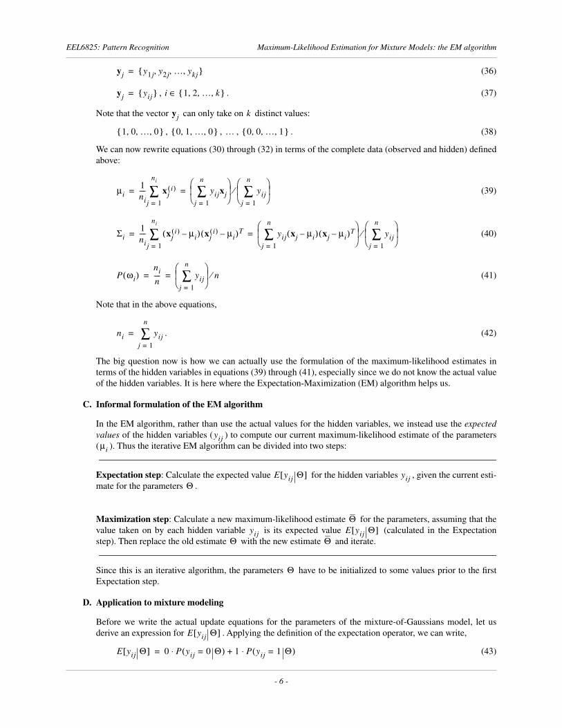
The big question now is how we can actually use the formulation of the maximum-likelihood estimates interms of the hidden variables in equations (39) through (41), especially since we do not know the actual valueof the hidden variables. It is here where the Expectation-Maximization (EM) algorithm helps us.
C. Informal formulation of the EM algorithm
In the EM algorithm, rather than use the actual values for the hidden variables, we instead use the
expectedvalues
of the hidden variables ( ) to compute our current maximum-likelihood estimate of the parameters( ). Thus the iterative EM algorithm can be divided into two steps:
Expectation step
: Calculate the expected value for the hidden variables , given the current esti-mate for the parameters .
Maximization step
: Calculate a new maximum-likelihood estimate for the parameters, assuming that thevalue taken on by each hidden variable is its expected value (calculated in the Expectationstep). Then replace the old estimate with the new estimate and iterate.
Since this is an iterative algorithm, the parameters have to be initialized to some values prior to the firstExpectation step.
D. Application to mixture modeling
Before we write the actual update equations for the parameters of the mixture-of-Gaussians model, let usderive an expression for . Applying the definition of the expectation operator, we can write,
(43)
y
j
y
1
j
y
2
j
…
y
kj
, , ,{ }
=
y
j
y
ij
{ }
=
i
1 2
…
k
, , ,{ }∈
y
j
k
1 0
…
0
, , ,{ }
0 1
…
0
, , ,{ }
…
0 0
…
1
, , ,{ }
µ
i
1
n
i
----
x
ji
( )
j
1
=
n
i
∑
y
ij
x
jj
1
=
n
∑
y
ijj
1
=
n
∑
⁄
= =
Σ
i
1
n
i
----
x
ji
( )
µ
i
–
( )
x
ji
( )
µ
i
–
( )
T
j
1
=
n
i
∑
y
ij
x
j
µ
i
–
( )
x
j
µ
i
–
( )
T
j
1
=
n
∑
y
ijj
1
=
n
∑
⁄
= =
P
ω
i
( )
n
i
n
----
y
ijj
1
=
n
∑
n
⁄
= =
n
i
y
ijj
1
=
n
∑
=
y
ij
µ
i
E y
ij
Θ[ ]
y
ij
Θ
Θ
y
ij
E y
ij
Θ[ ]
Θ
Θ
Θ
E y
ij
Θ[ ]
E y
ij
Θ[ ]
0
P y
ij
0
=
Θ( )⋅
1
P y
ij
1
=
Θ( )⋅
+=

EEL6825: Pattern Recognition Maximum-Likelihood Estimation for Mixture Models: the EM algorithm
- 7 -
(44)
Let us rewrite the right-hand-side of equation (44):
(45)
so that:
(46)
Now, let us write in a form that we can compute. Applying Bayes Theorem,
(47)
(48)
Note that equation (48) completely defines in terms of computable functions [see equations (1) and(4)]. Thus, we can now write the iterative EM equations by combining equation (46) with equations (39)through (41):
, (49)
, (50)
, (51)
It is important to remember that is computed in terms of the current parameter estimates ,while the left-hand sides of equations (49) through (51) give a new set of parameter estimates. These equa-tions should be intuitively appealing, since the contribution of each to the th component density isweighted by the probability that belongs to the th component density.
1
E. Another look at simple mixture modeling example
Let us take another look at the example from Section 1(C)-(D). There we attempted to solve for the maxi-mum-likelihood estimates of the means starting from,
[equation (21)]. (52)
This formulation resulted in the following two equations:
1. Note that in computing new estimates for , we use the new estimates of the means ; while it may not be immediately obvious why we do this, in Section 5, we derive this update rule directly from the formal statement of the EM algorithm.
E y
ij
Θ[ ]
P y
ij
1
=
Θ( )
=
P y
ij
1
=
Θ( )
P
ω
i
x
j
Θ,( )
=
E y
ij
Θ[ ]
P
ω
i
x
j
Θ,( )
=
P
ω
i
x
j
Θ,( )
P
ω
i
x
j
Θ,( )
p
x
j
Θ ω
i
,( )
P
ω
i
( )
p
x
j
Θ( )
-------------------------------------------
p
x
j
φ
i
( )
P
ω
i
( )
p
x
j
Θ( )
----------------------------------= =
E y
ij
Θ[ ]
p
x
j
φ
i
( )
P
ω
i
( )
p
x
j
Θ( )
----------------------------------=
E y
ij
Θ[ ]
µ
i
P
ω
i
x
j
Θ,( )
x
jj
1
=
n
∑
P
ω
i
x
j
Θ,( )
j
1
=
n
∑
--------------------------------------------=
i
1 2
…
k
, , ,{ }∈
Σ
i
P
ω
i
x
j
Θ,( )
x
j
µ
i
–
( )
x
j
µ
i
–
( )
T
j
1
=
n
∑
P
ω
i
x
j
Θ,( )
j
1
=
n
∑
-----------------------------------------------------------------------------------=
i
1 2
…
k
, , ,{ }∈
P
ω
i
( )
1
n
---
P
ω
i
x
j
Θ,( )
j
1
=
n
∑
=
i
1 2
…
k
, , ,{ }∈
P
ω
i
x
j
Θ,( )
Θ
x
j
i
x
j
i
Σ
i
µ
i
µ
1
µ
2
,{ }
p
X
Θ( )
ln
µ
1
µ
2
,( )
∇
0
=

EEL6825: Pattern Recognition Maximum-Likelihood Estimation for Mixture Models: the EM algorithm
- 8 -
, [equation (26)]. (53)
Equation (53) can be simplified using (47) above (Bayes Theorem),
(54)
, . (55)
Solving equation (55) for ,
(56)
Note that if we use equation (56) in an iterative manner, it is identical to the EM update rule in equation (49),which should be a little surprising, since the two results were arrived at from completely different formula-tions.
Below, we plot EM trajectories for the same data as in Section 1(D), and some different initial values for and (Figure 4, left plot, red lines). For these trajectories, the EM algorithm converges on average in about13 steps, which compares quite favorably to the gradient descent-algorithm, which converges on average inabout 50 steps for the same initial parameter values and a hand-optimized learning rate of (Figure4, right plot, blue lines).
The gradient-descent algorithm for statistical modeling suffers from two main deficiencies: (1) it convergesslowly, despite careful hand selection of the learning rate; and (2) it requires explicit computation of the gra-dient of the log-likelihood function , which the EM algorithm does not. Note that both theEM and gradient-descent algorithms are
not
guaranteed to converge to a
global
maximum of the log-likeli-hood function, only a
local
maximum, depending on initial parameter values. In fact, the gradient-descentalgorithm can fail to converge altogether, as shown in Figure 5. In Figure 5 we plot two EM and gradientdescent trajectories in parameter space with initial parameter values of and
p x
j
µ
i
( )
P
ω
i
( )
x
j
µ
i
–
( )
p x
j
µ
1
( )
P
ω
1
( )
p x
j
µ
2
( )
P
ω
2
( )
+--------------------------------------------------------------------------------
j
1
=
n
∑
0
=
i
1 2
,{ }∈
p x
j
µ
i
( )
P
ω
i
( )
p x
j
µ
1
( )
P
ω
1
( )
p x
j
µ
2
( )
P
ω
2
( )
+--------------------------------------------------------------------------------
P
ω
i
x
j
µ
1
µ
2
, ,( )
P
ω
i
x
j
Θ,( )
= =
P
ω
i
x
j
Θ,( )
x
j
µ
i
–
( )
j
1
=
n
∑
0
=
i
1 2
,{ }∈
µ
i
µ
i
P
ω
i
x
j
Θ,( )
x
jj
1
=
n
∑
P
ω
i
x
j
Θ,( )
j
1
=
n
∑
-------------------------------------------=
µ
1
µ
2
η
0.04
=
Figure 4
µ
2
µ
1
-6 -4 -2 0 2 4 6-6
-4
-2
0
2
4
6
µ
2
µ
1
EM convergence Gradient descent convergence
p
X
Θ( )
ln
µ
1
µ
2
,( )
∇
µ
1
µ
2
,{ }
15
–
15
,{ }
=

EEL6825: Pattern Recognition Maximum-Likelihood Estimation for Mixture Models: the EM algorithm
- 9 -
, respectively. Note that in the first instance, gradient descent requires 11,890 steps toconverge (compared to 9 for EM), while in the second instance, gradient descent fails to converge entirely,getting stuck in a part of the log-likelihood function where .
3. Generalized Formulation of Expectation-Maximization (EM) algorithm
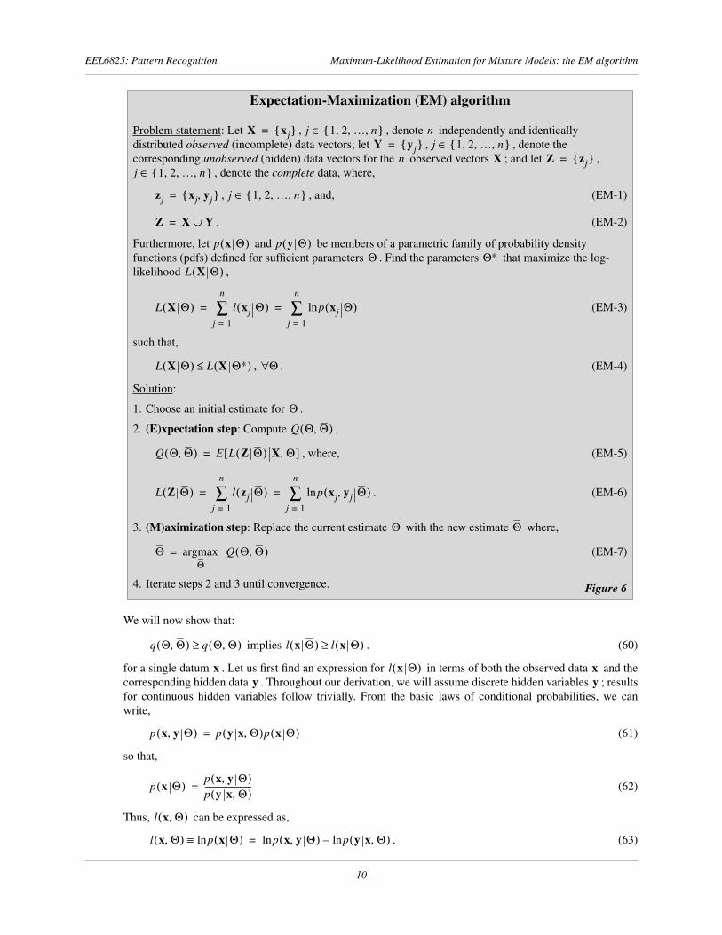
The previous section gives an intuitive, informal formulation of the EM algorithm, and shows how the EM algo-rithm can be used to solve the maximum-likelihood parameter estimation problem in mixture-of-Gaussians mod-eling. In this section, we formalize and generalize our previous discussion on the maximum-likelihoodestimation problem for data with hidden components. We start with a formal definition of the problem and thecorresponding EM algorithm, as stated in Figure 6 (next page).
This generalized formulation of the EM algorithm is not easy to understand. It does, however, describe a power-ful algorithm for maximum-likelihood estimation that is applicable not only for mixture-of-Gaussians modeling,but for vector quantization, general mixture modeling and hidden Markov models as well. The EM algorithm isparticularly applicable when the -function is easy to compute and is easier to maximize than maximizing thelog-likelihood directly. In the following two sections, we will first prove that maximizingthe -function also maximizes the log-likelihood function; that is, we will show that,
implies . (57)
Second, we will derive the EM solution for mixture-of-Gaussians modeling, starting with the general formulationin Figure 6; not surprisingly, we will see that this exercise will lead us to the same parameter update equations asthe informal statement of the EM algorithm did [see equations (49) through (51)].
4. Convergence proof for the EM algorithm
In this section, we will prove that maximizing the -function also maximizes the log-likelihood function; that is,we will show that,
implies . (58)
Below, we will break the proof into two steps. First, we will show that property (58) holds for a
single
datum .Then will generalize this result to multiple observations , .
A. Relating log-likelihood and -function for one observation
Let us denote,
. (59)
µ
1
µ
2
,{ }
10
–
15
,{ }
=
p
X
Θ( )
ln
µ
1
µ
2
,( )
∇
0
≈
-15 -12.5 -10 -7.5 -5 -2.5 00
2
4
6
8
10
12
14
-14 -12 -10 -8 -6 -4 -2 00
2
4
6
8
10
12
14
Figure 5
µ
2
µ
1
µ
2
µ
1
EM (red line, 9 steps)Gradient descent (blue line, 11,890 steps)
EM (red line, 12 steps)Gradient descent (blue line, fails)
Q
L
X
Θ( )
p
X
Θ( )
ln
=
Q
Q
Θ Θ,( )
Q
Θ Θ,( )≥
L
X
Θ( )
L
X|
Θ( )≥
Q
Q
Θ Θ,( )
Q
Θ Θ,( )≥
L
X
Θ( )
L
X|
Θ( )≥
x
X x
j
{ }
=
j
1 2
…
n
, , ,{ }∈
Q
q
Θ Θ,( )
E l
z
Θ( )
x
Θ,[ ]
=
EEL6825: Pattern Recognition Maximum-Likelihood Estimation for Mixture Models: the EM algorithm
- 10 -
We will now show that:
implies . (60)
for a single datum . Let us first find an expression for in terms of both the observed data and thecorresponding hidden data . Throughout our derivation, we will assume discrete hidden variables ; resultsfor continuous hidden variables follow trivially. From the basic laws of conditional probabilities, we canwrite,
(61)
so that,
(62)
Thus, can be expressed as,
. (63)
Expectation-Maximization (EM) algorithm
Problem statement: Let , , denote independently and identically distributed
observed
(incomplete) data vectors; let , , denote the corresponding
unobserved
(hidden) data vectors for the observed vectors ; and let , , denote the
complete
data, where,
, , and, (EM-1)
. (EM-2)
Furthermore, let and be members of a parametric family of probability density functions (pdfs) defined for sufficient parameters . Find the parameters that maximize the log-likelihood ,
(EM-3)
such that,
, . (EM-4)
Solution:
1. Choose an initial estimate for .
2.
(E)xpectation step
: Compute ,
, where, (EM-5)
. (EM-6)
3.
(M)aximization step
: Replace the current estimate with the new estimate where,
(EM-7)
4. Iterate steps 2 and 3 until convergence.
X x
j
{ }
=
j
1 2
…
n
, , ,{ }∈
n
Y y
j
{ }
=
j
1 2
…
n
, , ,{ }∈
n
X
Z z
j
{ }
=
j
1 2
…
n
, , ,{ }∈
z
j
x
j
y
j
,{ }
=
j
1 2
…
n
, , ,{ }∈
Z X Y
∪
=
p
x
Θ( )
p
y
Θ( )
Θ
Θ∗
L
X
Θ( )
L
X
Θ( )
l
x
j
Θ( )
j
1
=
n
∑
p
x
j
Θ( )
ln
j
1
=
n
∑
= =
L
X
Θ( )
L
X
Θ∗( )≤
Θ∀
Θ
Q
Θ Θ,( )
Q
Θ Θ,( )
E L
Z
Θ( )
X
Θ,[ ]
=
L
Z
Θ( )
l
z
j
Θ( )
j
1
=
n
∑
p
x
j
y
j
, Θ( )
ln
j
1
=
n
∑
= =
Θ
Θ
Θ
argmax
Θ
Q
Θ Θ,( )
=
Figure 6
q
Θ Θ,( )
q
Θ Θ,( )≥
l
x
Θ( )
l
x
Θ( )≥
x
l
x
Θ( )
x
y
y
p
x y
, Θ( )
p
y x
Θ,( )
p
x
Θ( )
=
p
x
Θ( )
p
x y
, Θ( )
p
y x
Θ,( )
------------------------=
l
x
Θ,( )
l
x
Θ,( )
p
x
Θ( )
ln
≡
p
x y
, Θ( )
ln
p
y x
Θ,( )
ln
–=

EEL6825: Pattern Recognition Maximum-Likelihood Estimation for Mixture Models: the EM algorithm
- 11 -
Now, consider two parameter vectors and . The expectation of the incomplete log-likelihood over the complete data conditioned on and is given by,
(64)
(65)
Let us pause and think about what is meant by the conditional expectation operator used inequations (65). First, consider some function for which is a known constant and is a vector ofdiscrete random variables. For such a function,
(66)
Note that we do not sum up over all possible values of because is known and constant. The conditionalexpected value is similarly given by,
(discrete variables ) (67)
Let us now derive expressions for each of the terms in equation (65). First consider term :
(68)
Note that in equation (68),
(69)
since the probability that assumes any of its possible values is equal to one. Therefore, equation (68)reduces to:
(70)
Next, consider term :
(71)
Finally, consider term :
(72)
Since we cannot simplify equation (72), let us denote it as :
. (73)
Let us now substitute equations (70), (71) and (73) into (65):
(74)
Equation (74) gives us a relationship between the log-likelihood of with respect to the new parameter vec-tor and the -function for a single observation. In the next section, we will exploit that relation-ship to show that implies .
Θ
Θ
l
x
Θ,( )
z x y
,{ }
=
x
Θ
E l
x
Θ,( )
x
Θ,[ ]
E p
x y
, Θ( )
ln
p
y x
Θ,( )
ln
–
{ }
x
Θ,[ ]
=
E l
x
Θ,( )
x
Θ,[ ]
E p
x y
, Θ( )
ln
x
Θ,[ ]
E p
y x
Θ,( )
ln
x
Θ,[ ]
–=
a
( )
b
( )
c
( )
E
•
x
Θ,[ ]
f
x y
,( )
x
y
E f
x y
,( )[ ]
f
x y
,( )
p
y
( )
y
∑
≡
x
x
E f
x y
,( )
x
Θ,[ ]
E f
x y
,( )
x
Θ,[ ]
f
x y
,( )
p
y x
Θ,( )
y
∑
≡
y
a
( )
E l
x
Θ,( )
x
Θ,[ ]
E p
x
Θ( )
ln
x
Θ,[ ]
=
p
x
Θ( )
ln
[ ]
p
y x
Θ,( )
y
∑
=
p
x
Θ( )
ln
p
y x
Θ,( )
y
∑
=
p
y x
Θ,( )
y
∑
1
=
y
E l
x
Θ,( )
x
Θ,[ ]
p
x
Θ( )
ln
l
x
Θ,( )
= =
b
( )
E p
x y
, Θ( )
ln
x
Θ,[ ]
E l
z
Θ( )
x
Θ,[ ]
q
Θ Θ,( )≡
=
c
( )
E p
y x
Θ,( )
ln
x
Θ,[ ]
p
y x
Θ,( )
ln
p
y x
Θ,( )
y
∑
=
h
Θ Θ,( )
h
Θ Θ,( )
p
y x
Θ,( )
ln
p
y x
Θ,( )
y
∑
=
l
x
Θ,( )
q
Θ Θ,( )
h
Θ Θ,( )
–=
x
Θ
Q
q
Θ Θ,( )
q
Θ Θ,( )
q
Θ Θ,( )≥
l
x
Θ( )
l
x
Θ( )≥

EEL6825: Pattern Recognition Maximum-Likelihood Estimation for Mixture Models: the EM algorithm
- 12 -
B. Jensen’s inequality
We will now show that,
. (75)
Equation (75) is known as
Jensen’s inequality
. Let us begin with the definition of :
[same as (73)] (76)
For :
(77)
Let us now subtract (77) from (76):
(78)
(79)
(80)
Now, we observe the following inequality (as depicted in Figure 7):
, . (81)
Since we can combine (80) and (81):
(82)
(83)
(84)
(85)
Note that in equation (85),
(86)
h
Θ Θ,( )
h
Θ Θ,( )≤
h
Θ Θ,( )
h
Θ Θ,( )
p
y x
Θ,( )
ln
p
y x
Θ,( )
y
∑
=
h
Θ Θ,( )
h
Θ Θ,( )
p
y x
Θ,( )
ln
p
y x
Θ,( )
y
∑
=
h
Θ Θ,( )
h
Θ Θ,( )
–
p
y x
Θ,( )
ln
p
y x
Θ,( )
y
∑
p
y x
Θ,( )
ln
p
y x
Θ,( )
y
∑
–=
h
Θ Θ,( )
h
Θ Θ,( )
–
p
y x
Θ,( )
ln
p
y x
Θ,( )
p
y x
Θ,( )
ln
p
y x
Θ,( )
–
[ ]
y
∑
=
h
Θ Θ,( )
h
Θ Θ,( )
–
p
y x
Θ,( )
p
y x
Θ,( )
------------------------
ln
p
y x
Θ,( )
y
∑
=
x
ln
x
1
–
( )≤
x
∀
0 1 2 3 4 5
-2
-1
0
1
2
3
4
Figure 7
x
1
–
( )
x
ln
p
y x
Θ,( )
0
≥
h
Θ Θ,( )
h
Θ Θ,( )
–
p
y x
Θ,( )
p
y x
Θ,( )
------------------------
ln
p
y x
Θ,( )
y
∑
p
y x
Θ,( )
p
y x
Θ,( )
------------------------
1
–
p
y x
Θ,( )
y
∑
≤
=
h
Θ Θ,( )
h
Θ Θ,( )
–
p
y x
Θ,( )
p
y x
Θ,( )
------------------------
1
–
p
y x
Θ,( )
y
∑
≤
h
Θ Θ,( )
h
Θ Θ,( )
–
p
y x
Θ,( )
p
y x
Θ,( )
–
[ ]
y
∑
≤
h
Θ Θ,( )
h
Θ Θ,( )
–
p
y x
Θ,( )
y
∑
p
y x
Θ,( )
y
∑
–
≤
p
y x
Θ,( )
y
∑
p
y x
Θ,( )
y
∑
1
= =

EEL6825: Pattern Recognition Maximum-Likelihood Estimation for Mixture Models: the EM algorithm
- 13 -
so that (85) reduces to:
(87)
(88)
C. Corollary to Jensen’s inequality
Recalling equation (74),
(89)
note that Jensen’s inequality directly leads to the following corollary:
implies . (90)
In other words, maximizing the -function for a single data point implies an increase in the log-likelihoodfunction .
D. Multiple observations
We now want to generalize the result of the previous section for a single data to multiple data ,. From equations (EM-3) and (63),
(91)
(92)
Changing to , and applying the conditional expectation operator to equation (92), we get,
(93)
Let us now expand each of the terms in equation (93). First, we compute :
(94)
The second term is, by definition (EM-5):
(95)
In terms of functions ,
, (96)
h
Θ Θ,( )
h
Θ Θ,( )
–
0
≤
h
Θ Θ,( )
h
Θ Θ,( )≤
l
x
Θ,( )
q
Θ Θ,( )
h
Θ Θ,( )
–=
q
Θ Θ,( )
q
Θ Θ,( )≥
l
x
Θ( )
l
x
Θ( )≥
Q
l
x
Θ( )
x
X x
j
{ }
=
j
1 2
…
n
, , ,{ }∈
L
X
Θ( )
p
x
j
Θ( )
ln
j
1
=
n
∑
p
x
j
y
j
, Θ( )
ln
p
y
j
x
j
Θ,( )
ln
j
1
=
n
∑
–
j
1
=
n
∑
= =
L
X
Θ( )
L
Z
Θ( )
L
Y X
Θ,( )
–=
Θ
Θ
E
•
X
Θ,[ ]
E L
X
Θ( )
X
Θ,[ ]
E L
Z
Θ( )
X
Θ,[ ]
E L
Y X
Θ,( )
X
Θ,[ ]
–=
E L
X
Θ( )
X
Θ,[ ]
E L
X
Θ( )
X
Θ,[ ]
E p
x
j
Θ( )
ln
j
1
=
n
∑
X
Θ,
=
p
x
j
Θ( )
p
y
l
x
l
Θ,( )
l
1
=
n
∏
ln
j
1
=
n
∑
y
∑
=
p
x
j
Θ( )
p
y
l
x
l
Θ,( )
y
l
∑
l
1
=
n
∏
ln
j
1
=
n
∑
=
p
x
j
Θ( )
ln
j
1
=
n
∑
=
L
X
Θ( )
=
Q
Θ Θ,( )
E L
Z
Θ( )
X
Θ,[ ]≡
q
j
Θ Θ,( )
q
j
Θ Θ,( )
E l
z
j
Θ( )
x
j
Θ,[ ]≡

EEL6825: Pattern Recognition Maximum-Likelihood Estimation for Mixture Models: the EM algorithm
- 14 -
(97)
Finally, we compute . Similar to equation (97),
(98)
. (99)
Combining the above results, we get,
(100)
(101)
Since equation (101) simply represents a summation over individual data , we observe that the sameresult holds as before, namely:
implies . (102)
Q
Θ Θ,( )
E p
x
j
y
j
, Θ( )
ln
j
1
=
n
∑
X
Θ,
=
p
x
j
y
j
, Θ( )
p
y
l
x
l
Θ,( )
l
1
=
n
∏
ln
j
1
=
n
∑
y
∑
=
p
x
j
y
j
, Θ( )
p
y
j
x
j
Θ,( )
ln
y
j
∑
p
y
l
x
l
Θ,( )
y
l
∑
l j
≠
∏
j
1
=
n
∑
=
p
x
j
y
j
, Θ( )
p
y
j
x
j
Θ,( )
ln
y
j
∑
j
1
=
n
∑
=
p
z
j
Θ( )
p
y
j
x
j
Θ,( )
ln
y
j
∑
j
1
=
n
∑
=
q
j
Θ Θ,( )
j
1
=
n
∑
≡
H
Θ Θ,( )
E L
Y X
Θ,( )
X
Θ,[ ]
=
H
Θ Θ,( )
E p
y
j
x
j
Θ,( )
ln
j
1
=
n
∑
X
Θ,
=
p
y
j
x
j
Θ,( )
p
y
l
x
l
Θ,( )
l
1
=
n
∏
ln
j
1
=
n
∑
y
∑
=
p
y
j
x
j
Θ,( )
p
y
j
x
j
Θ,( )
ln
y
j
∑
p
y
l
x
l
Θ,( )
y
l
∑
l j
≠
∏
j
1
=
n
∑
=
p
y
j
x
j
Θ,( )
p
y
j
x
j
Θ,( )
ln
y
j
∑
j
1
=
n
∑
=
h
j
Θ Θ,( )
j
1
=
n
∑
≡
h
j
Θ Θ,( )
E p
y
j
x
j
Θ,( )
x
j
Θ,
ln
[ ]
=
L
X
Θ,( )
Q
Θ Θ,( )
H
Θ Θ,( )
–=
p
x
j
Θ( )
ln
j
1
=
n
∑
q
j
Θ Θ,( )
j
1
=
n
∑
h
j
Θ Θ,( )
j
1
=
n
∑
–=
x
j
{ }
Q
Θ Θ,( )
Q
Θ Θ,( )≥
L
X
Θ( )
L
X|
Θ( )≥
EEL6825: Pattern Recognition Maximum-Likelihood Estimation for Mixture Models: the EM algorithm
- 15 -
E. Concluding thoughts
We have now shown that improving the -function at each step of the EM algorithm will also improve thelog-likelihood of the data given the new parameters. This is an important result, since it tells us that every stepof an EM update for a specific problem will always improve the current log-likelihood until wereach a local maximum on the log-likelihood function. In the next section, we will derive the EM updateequations for mixture-of-Gaussians modeling.
5. Maximum-likelihood solution for mixture-of-Gaussians modeling
A. Problem statement
Assume you are given a set of identically and independently distributed -dimensional data ,, drawn from the probability density function,
(103)
where denotes a parameter vector fully specifying the th component density , denotes theprobability (i.e. weight) of the th component density ,
(104)
, (105)
, and, (106)
, . (107)
Compute the maximum-likelihood parameter estimates for the parameters .
B. Definition of hidden variables
Solution: Let us begin with the definition of the EM algorithm. First, we need to define our hidden variables.Second, we need to perform the
expectation
step of the EM algorithm for this problem; that is, we need tocompute as defined in equation (EM-5). Third, we need to perform the
maximization
step of theEM algorithm, as indicated in equation (EM-7).
Let us define the
hidden
data vector corresponding to the
observed
datum as,
(108)
where the are discrete random variables with the following possible values,
(109)
Note that the vector can only take on distinct values:
, , , . (110)
Finally, let denote the vector where and all other , , and let denote the th complete data vector.
C. Expectation step
Previously, we shown that the -function defined in (EM-5),
Q
L
X
Θ( )
d
X x
j
{ }
=
j
1 2
…
n
, , ,{ }∈
p
x
Θ( )
p
x
φ
i
( )
P
ω
i
( )
i
1
=
k
∑
=
φ
i
i
p
x
φ
i
( )
P
ω
i
( )
i
p
x
φ
i
( )
p
x
φ
i
( )
p
x
µ
i
Σ
i
,( )
12
π( )
d
2
⁄
Σ
i
1 2
/
-----------------------------------
12
---
x
µ
i
–
( )
T
–
Σ
i
1
–
x
µ
i
–
( )
exp
N
x
µ
i
Σ
i
, ,[ ]
= = =
φ
i
µ
i
Σ
i
,{ }
=
Θ
i
φ
i
P
ω
i
( ),{ }
=
Θ Θ
i
{ }
=
i
1 2
…
k
, , ,{ }∈
Θ
Q
Θ Θ,( )
y
j
x
j
y
j
y
1
j
y
2
j
…
y
kj
, , ,{ }
=
y
ij
y
ij
1
x
j
belongs to class
ω
i
0
otherwise
≡
y
j
k
1 0
…
0
, , ,{ }
0 1
…
0
, , ,{ }
…
0 0
…
1
, , ,{ }
y
ji
( )
y
j
y
ij
1
=
y
lj
0
=
l
∀
i
≠
z
j
x
j
y
j
,{ }
=
j
Q
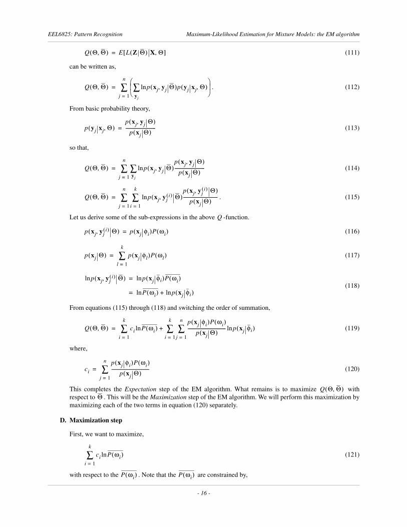
EEL6825: Pattern Recognition Maximum-Likelihood Estimation for Mixture Models: the EM algorithm
- 16 -
(111)
can be written as,
. (112)
From basic probability theory,
(113)
so that,
(114)
. (115)
Let us derive some of the sub-expressions in the above -function.
(116)
(117)
(118)
From equations (115) through (118) and switching the order of summation,
(119)
where,
(120)
This completes the
Expectation
step of the EM algorithm. What remains is to maximize withrespect to . This will be the
Maximization
step of the EM algorithm. We will perform this maximization bymaximizing each of the two terms in equation (120) separately.
D. Maximization step
First, we want to maximize,
(121)
with respect to the . Note that the are constrained by,
Q
Θ Θ,( )
E L
Z
Θ( )
X
Θ,[ ]
=
Q
Θ Θ,( )
p
x
j
y
j
, Θ( )
p
y
j
x
j
Θ,( )
ln
y
j
∑
j
1
=
n
∑
=
p
y
j
x
j
Θ,( )
p
x
j
y
j
, Θ( )
p
x
j
Θ( )
---------------------------=
Q
Θ Θ,( )
p
x
j
y
j
, Θ( )
p
x
j
y
j
, Θ( )
p
x
j
Θ( )
---------------------------
ln
y
j
∑
j
1
=
n
∑
=
Q
Θ Θ,( )
p
x
j
y
ji
( )
, Θ( )
p
x
j
y
ji
( )
, Θ( )
p
x
j
Θ( )
-------------------------------
ln
i
1
=
k
∑
j
1
=
n
∑
=
Q
p
x
j
y
ji
( )
, Θ( )
p
x
j
φ
i
( )
P
ω
i
( )
=
p
x
j
Θ( )
p
x
j
φ
l
( )
P
ω
l
( )
l
1
=
k
∑
=
p
x
j
y
ji
( )
, Θ( )
ln
p
x
j
φ
i
( )
P
ω
i
( )
ln
=
P
ω
i
( )
ln
p
x
j
φ
i
( )
ln
+=
Q
Θ Θ,( )
c
i
P
ω
i
( )
ln
i
1
=
k
∑
p
x
j
φ
i
( )
P
ω
i
( )
p
x
j
Θ( )
----------------------------------
j
1
=
n
∑
p
x
j
φ
i
( )
ln
i
1
=
k
∑
+=
c
i
p
x
j
φ
i
( )
P
ω
i
( )
p
x
j
Θ( )
----------------------------------
j
1
=
n
∑
=
Q
Θ Θ,( )
Θ
c
i
P
ω
i
( )
ln
i
1
=
k
∑
P
ω
i
( )
P
ω
i
( )

EEL6825: Pattern Recognition Maximum-Likelihood Estimation for Mixture Models: the EM algorithm
- 17 -
(122)
Remember from your basic calculus, that this type of
constrained optimization
can be performed through themethod of
Lagrange multipliers
.
[Note: In general, a function,
(123)
with constraint,
(124)
is maximized by maximizing the augmented objective function ,
, (125)
where is called the Lagrange multiplier.]
In our case,
(126)
and, switching the index of summation from to ,
(127)
Taking the derivative of (127) with respect to ,
(128)
(129)
Let us now sum equation (129) over all ,and solve for :
(130)
(131)
Note, however that,
(132)
Therefore, equation (131) simplifies to,
(133)
Combining equations (129) and (133),
P
ω
i
( )
i
1
=
k
∑
1
=
f
x
( )
g
x
( )
a
=
h
x
( )
h
x
( )
f
x
( ) λ
g
x
( )
+=
λ
h c
i
P
ω
i
( )
ln
i
1
=
k
∑
λ
P
ω
i
( )
i
1
=
k
∑
+=
i
l
h c
l
P
ω
l
( )
ln
λ
P
ω
l
( )
+
[ ]
l
1
=
k
∑
=
P
ω
i
( )
∂
h
∂
P
ω
i
( )
-----------------
c
i
P
ω
i
( )
--------------
λ
+
0
= =
c
i
λ
P
ω
i
( )
+
0
=
i
λ
c
l
λ
P
ω
l
( )
+
[ ]
l
1
=
k
∑
0
=
λ
c
ll
1
=
k
∑
P
ω
l
( )
l
1
=
k
∑
⁄
–=
P
ω
l
( )
l
1
=
k
∑
1
=
λ
c
ll
1
=
k
∑
–=

EEL6825: Pattern Recognition Maximum-Likelihood Estimation for Mixture Models: the EM algorithm
- 18 -
(134)
(135)
Inserting equation (120) into (135), and switching the order of summation in the denominator,
(136)
(137)
Note that,
(138)
Therefore, equation (137) simplifies to,
, (139)
Thus, equation (139) gives us the EM iterative update rule for estimating the priors . The maximizationof the second term in equation (119) proceeds by setting the gradient with respect to of,
(140)
equal to zero,
(141)
and solving for . In order to compute the gradients,
(142)
for the Gaussian distribution,
(143)
c
i
c
ll
1
=
k
∑
P
ω
i
( )
–
0
=
P
ω
i
( )
c
i
c
ll
1
=
k
∑
--------------=
P
ω
i
( )
p
x
j
φ
i
( )
P
ω
i
( )
p
x
j
Θ( )
----------------------------------
j
1
=
n
∑
p
x
j
φ
l
( )
P
ω
l
( )
p
x
j
Θ( )
----------------------------------
l
1
=
k
∑
j
1
=
n
∑
-------------------------------------------------------=
P
ω
i
( )
p
x
j
φ
i
( )
P
ω
i
( )
p
x
j
Θ( )
----------------------------------
j
1
=
n
∑
p
x
j
φ
l
( )
P
ω
l
( )
l
1
=
k
∑
p
x
j
Θ( )
---------------------------------------------
j
1
=
n
∑
-------------------------------------------------------=
p
x
j
φ
l
( )
P
ω
l
( )
l
1
=
k
∑
p
x
j
Θ( )
---------------------------------------------
p
x
j
Θ( )
p
x
j
Θ( )
-------------------
1
= =
P
ω
i
( )
1
n
---
p
x
j
φ
i
( )
P
ω
i
( )
p
x
j
Θ( )
----------------------------------
j
1
=
n
∑
1
n
---
P
ω
i
x
j
Θ,( )
j
1
=
n
∑
= =
i
1 2
…
k
, , ,{ }∈
P
ω
i
( )
φ
i
p
x
j
φ
l
( )
P
ω
l
( )
p
x
j
Θ( )
----------------------------------
j
1
=
n
∑
p
x
j
φ
l
( )
ln
l
1
=
k
∑
p
x
j
φ
l
( )
P
ω
l
( )
p
x
j
Θ( )
----------------------------------
j
1
=
n
∑
p
x
j
φ
l
( )
ln
l
1
=
k
∑
φ
i
∇
p
x
j
φ
i
( )
P
ω
i
( )
p
x
j
Θ( )
----------------------------------
j
1
=
n
∑
p
x
j
φ
i
( )
φ
i
∇
p
x
j
φ
i
( )
---------------------------
0
= =
φ
i
p
x
j
φ
i
( )
φ
i
∇
p
x
j
φ
i
( )
p
x
j
µ
i
Σ
i
,( )
12
π( )
d
2
⁄
Σ
i
1 2
/
-----------------------------------
12
---
x
j
µ
i
–
( )
T
–
Σ
i
1
–
x
j
µ
i
–
( )
exp
N
x
j
µ
i
Σ
i
, ,[ ]≡
= =

EEL6825: Pattern Recognition Maximum-Likelihood Estimation for Mixture Models: the EM algorithm
- 19 -
we will need to compute,
and (144)
separately. In order to undertake this, we will make use of the following results from linear algebra:
(145)
(146)
(147)
(148)
where is a -dimensional vector, and is a matrix. Note that if is symmetric, then equation(145) reduces to,
(149)
and equation (147) reduces to,
. (150)
Given these identities from linear algebra, we can now compute the gradients in (144). First, for the meanvector ,
(151)
From equation (149),
(152)
(Here we drop the indices , and the over bar for notational simplicity.)
(153)
Reinserting the problem-specific notation,
(154)
We can now solve for . Combining equation (141), (143) and (154),
(155)
(156)
, . (157)
For the covariance matrices , rather than derive,
p
x
j
φ
i
( )
µ
i
∇
p
x
j
φ
i
( )
Σ
i
∇
b
T
Ab
( )
b
∇
Ab A
T
b
+=
b
T
Ab
( )
A
∇
bb
T
=
A
A
∇
A
T
( )
1
–
A
=
A
1
–
A
1
–
=
b
d
A
d d
×
A
b
T
Ab
( )
b
∇
2
Ab
=
A
A
∇
A
1
–
A
=
µ
i
p
x
j
φ
i
( )
µ
i
∇
N
x
j
µ
i
Σ
i
, ,[ ]
µ
i
∇
=
N
x
µ Σ, ,[ ]
µ
∇
N
x
µ Σ, ,[ ]
12
---
x
µ
–
( )
T
–
Σ
1
–
x
µ
–
( )
µ
∇
=
i
j
N
x
µ Σ, ,[ ]
µ
∇
N
x
µ Σ, ,[ ]Σ
1
–
x
µ
–
( )
=
N
x
j
µ
i
Σ
i
, ,[ ]
µ
i
∇
N
x
j
µ
i
Σ
i
, ,[ ]Σ
i
1
–
x
j
µ
i
–
( )
=
µ
i
p
x
j
φ
i
( )
P
ω
i
( )
p
x
j
Θ( )
----------------------------------
j
1
=
n
∑
p
x
j
φ
i
( )
µ
i
∇
p
x
j
φ
i
( )
----------------------------
0
=
p
x
j
φ
i
( )
P
ω
i
( )
p
x
j
Θ( )
----------------------------------
j
1
=
n
∑
Σ
i
1
–
x
j
µ
i
–
( )[ ]
0
=
µ
i
p
x
j
φ
i
( )
P
ω
i
( )
p
x
j
Θ( )
----------------------------------
x
jj
1
=
n
∑
p
x
j
φ
i
( )
P
ω
i
( )
p
x
j
Θ( )
----------------------------------
j
1
=
n
∑
--------------------------------------------------
P
ω
i
x
j
Θ,( )
x
jj
1
=
n
∑
P
ω
i
x
j
Θ,( )
j
1
=
n
∑
--------------------------------------------= =
i
1 2
…
k
, , ,{ }∈
Σ
i

EEL6825: Pattern Recognition Maximum-Likelihood Estimation for Mixture Models: the EM algorithm
- 20 -
(158)
we will compute,
(159)
instead, because it will be a little easier. (During the derivation, we will again drop the problem specific nota-tion.) Using the product and chain rules for differentiation,
(160)
Note that we can write,
(161)
so that equation (160) reduces to,
(162)
where,
[see equation (146)] (163)
and [see equations (148) and (150)],
(164)
Combining equations (162), (163) and (164),
(165)
(166)
Reinserting the problem-specific notation,
(167)
we can now solve for . Combining equation (141), (143) and (167),
p
x
j
φ
i
( )
Σ
i
∇
p
x
j
φ
i
( )
Σ
i
1
–
∇
N
x
j
µ
i
Σ
i
, ,[ ]
Σ
i
1
–
∇
=
N
x
µ Σ, ,[ ]
Σ
1
–
∇
N
x
µ Σ, ,[ ]
12
---
x
µ
–
( )
T
–
Σ
1
–
x
µ
–
( )
Σ
1
–
∇
+=
12
π( )
d
2
⁄
-------------------
12
---
x
µ
–
( )
T
–
Σ
1
–
x
µ
–
( )
exp
Σ
1 2
⁄
–
[ ]
Σ
1
–
∇
12
π( )
d
2
⁄
-------------------
12
---
x
µ
–
( )
T
–
Σ
1
–
x
µ
–
( )
exp
N
x
µ Σ, ,[ ] Σ
1 2
/
=
N
x
µ Σ, ,[ ]
Σ
1
–
∇
N
x
µ Σ, ,[ ]
12
---
x
µ
–
( )
T
–
Σ
1
–
x
µ
–
( )
Σ
1
–
∇
N
x
µ Σ, ,[ ] Σ
1 2
/
Σ
1 2
⁄
–
[ ]
Σ
1
–
∇
+=
12
---
x
µ
–
( )
T
–
Σ
1
–
x
µ
–
( )
Σ
1
–
∇
12
---
x
µ
–
( )
T
–
x
µ
–
( )
=
Σ
1 2
⁄
–
[ ]
Σ
1
–
∇ Σ
1
–
1 2
⁄
[ ]
Σ
1
–
∇
=
12
---
Σ
1
–
1 2
/–
Σ
1
–
Σ
1
–
∇
=
12
---
Σ
1
–
1
–
2
⁄
Σ Σ
1
–
=
12
---
Σ
1 2
⁄
Σ Σ
1
–
=
12
---
Σ
1 2
⁄
–
Σ
=
N
x
µ Σ, ,[ ]
Σ
1
–
∇
12
---
N
x
µ Σ, ,[ ]
x
µ
–
( )
x
µ
–
( )
T
–
12
---
N
x
µ Σ, ,[ ]Σ
+=
N
x
µ Σ, ,[ ]
Σ
1
–
∇
12
---
N
x
µ Σ, ,[ ] Σ
x
µ
–
( )
x
µ
–
( )
T
–
{ }
=
N
x
j
µ
i
Σ
i
, ,[ ]
Σ
i
1
–
∇
12
---
N
x
j
µ
i
Σ
i
, ,[ ] Σ
i
x
j
µ
i
–
( )
x
j
µ
i
–
( )
T
–
{ }
=
Σ
i
EEL6825: Pattern Recognition Maximum-Likelihood Estimation for Mixture Models: the EM algorithm
- 21 -
(168)
(169)
(170)
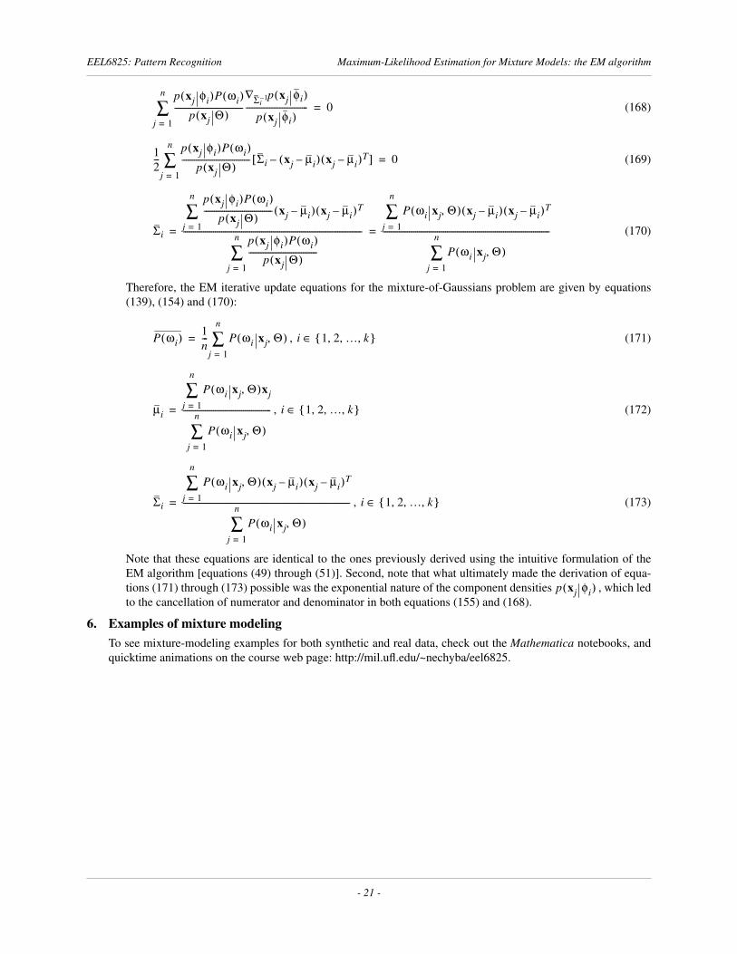
Therefore, the EM iterative update equations for the mixture-of-Gaussians problem are given by equations(139), (154) and (170):
, (171)
, (172)
, (173)
Note that these equations are identical to the ones previously derived using the intuitive formulation of theEM algorithm [equations (49) through (51)]. Second, note that what ultimately made the derivation of equa-tions (171) through (173) possible was the exponential nature of the component densities , which ledto the cancellation of numerator and denominator in both equations (155) and (168).
6. Examples of mixture modeling
To see mixture-modeling examples for both synthetic and real data, check out the
Mathematica
notebooks, andquicktime animations on the course web page: http://mil.ufl.edu/~nechyba/eel6825.
p
x
j
φ
i
( )
P
ω
i
( )
p
x
j
Θ( )
----------------------------------
j
1
=
n
∑
p
x
j
φ
i
( )
Σ
i
1
–
∇
p
x
j
φ
i
( )
-------------------------------
0
=
12
---
p
x
j
φ
i
( )
P
ω
i
( )
p
x
j
Θ( )
----------------------------------
j
1
=
n
∑
Σ
i
x
j
µ
i
–
( )
x
j
µ
i
–
( )
T
–
[ ]
0
=
Σ
i
p
x
j
φ
i
( )
P
ω
i
( )
p
x
j
Θ( )
----------------------------------
x
j
µ
i
–
( )
x
j
µ
i
–
( )
T
j
1
=
n
∑
p
x
j
φ
i
( )
P
ω
i
( )
p
x
j
Θ( )
----------------------------------
j
1
=
n
∑
-----------------------------------------------------------------------------------------
P
ω
i
x
j
Θ,( )
x
j
µ
i
–
( )
x
j
µ
i
–
( )
T
j
1
=
n
∑
P
ω
i
x
j
Θ,( )
j
1
=
n
∑
-----------------------------------------------------------------------------------= =
P
ω
i
( )
1
n
---
P
ω
i
x
j
Θ,( )
j
1
=
n
∑
=
i
1 2
…
k
, , ,{ }∈
µ
i
P
ω
i
x
j
Θ,( )
x
jj
1
=
n
∑
P
ω
i
x
j
Θ,( )
j
1
=
n
∑
--------------------------------------------=
i
1 2
…
k
, , ,{ }∈
Σ
i
P
ω
i
x
j
Θ,( )
x
j
µ
i
–
( )
x
j
µ
i
–
( )
T
j
1
=
n
∑
P
ω
i
x
j
Θ,( )
j
1
=
n
∑
-----------------------------------------------------------------------------------=
i
1 2
…
k
, , ,{ }∈
p
x
j
φ
i
( )