Embed Size (px)
Citation preview
Production and Cost Analysis I 12
Production and Cost Analysis I
Production is not the application of
tools to materials, but logic to work.
— Peter Drucker
CHAPTER 12
Copyright © 2010 by the McGraw-Hill Companies, Inc. All rights reserved.McGraw-Hill/Irwin

Production and Cost Analysis I 12
Maximizing Profit
• The goal of a firm is to maximize profits
• Profit = Total Revenue – Total Cost
12-2

Production and Cost Analysis I 12
Explicit versus Implicit Costs
• Explicit cost =money paid out (rent, wages, etc.)
• Implicit cost=opportunity cost of the factors of production used by the firm
12-3

Production and Cost Analysis I 12
Economic versus Accounting Profit
• Economists and accountants measure profit differently
• Unlike accountants, economists also consider implicit costs (the opportunity cost of what they could have done instead)
McGraw-Hill/Irwin Colander, Economics 4

Production and Cost Analysis I 12
Economic versus Accounting Profit
• Economists focus on both explicit and implicitcosts and revenue
• Economic profit = (explicit + implicit revenue) – (explicit + implicit cost)
• Accountants focus on explicit costs and revenues
• Accounting profit = explicit revenue –explicit cost
McGraw-Hill/Irwin Colander, Economics 5

Production and Cost Analysis I 12
Economic versus Accounting Profit
• When discussing costs, if a firm is making zeroeconomic profit they are always making a positive accounting profit
• This is because accounting profit does not take into consideration the opportunity cost of what they could have done instead
McGraw-Hill/Irwin Colander, Economics 6

Production and Cost Analysis I 12
Short run versus Long run
McGraw-Hill/Irwin Colander, Economics 7
• In the short run a firm is limited in regard to what production decisions it can make• Some inputs are fixed and cannot be
changed
• In the long run all inputs are variable inputs and can be changed

Production and Cost Analysis I 12
The Production Function
• The production function tells the maximum amount of output that can be derived from a given number of inputs
• Note it has three stages
McGraw-Hill/Irwin Colander, Economics 8

Production and Cost Analysis I 12
Graphing a Production Function Q
Increasing marginal productivity
Diminishingmarginal productivity
DiminishingAbsolute productivity
Number of workers
TP
A production function is the
relationship between then inputs and the
outputs
32
26
20
14
8
2
1 2 3 4 5 6 7 8 9 10
12-9

Production and Cost Analysis I 12
Law of Diminishing Marginal Productivity
• Law of diminishing marginal productivity: as more of a variable input is added to an existing fixed input, after some point the additional output from the additional input will fall
McGraw-Hill/Irwin Colander, Economics 10

Production and Cost Analysis I 12
Law of Diminishing Marginal Productivity
# of
workers
Total
Output
Marginal
Product
Average
Product
0 04
6
7
6
5
3
1
0
-2
-5
---
1 4 4
2 10 5
3 17 5.7
4 23 5.8
5 28 5.6
6 31 5.2
7 32 4.6
8 32 4.0
9 30 3.3
10 25 2.5
Increasing marginal productivity
Diminishingmarginal productivity
DiminishingAbsolute productivity
12-11

Production and Cost Analysis I 12
The Costs of Production
• Fixed costs (FC) are those that are spent and cannot be changed in the period of time under consideration
• In the short run, a number of inputs and their costs will be fixed
• In the long run, there are NO fixed costs since all inputs are variable
12-12

Production and Cost Analysis I 12
The Costs of Production
• Variable costs (VC) are costs that change as output changes
• Workers are an example of VC
• Total cost (TC) is the sum of the variable and fixed costs
• TC = FC + VC
McGraw-Hill/Irwin Colander, Economics 13
Production and Cost Analysis I 12
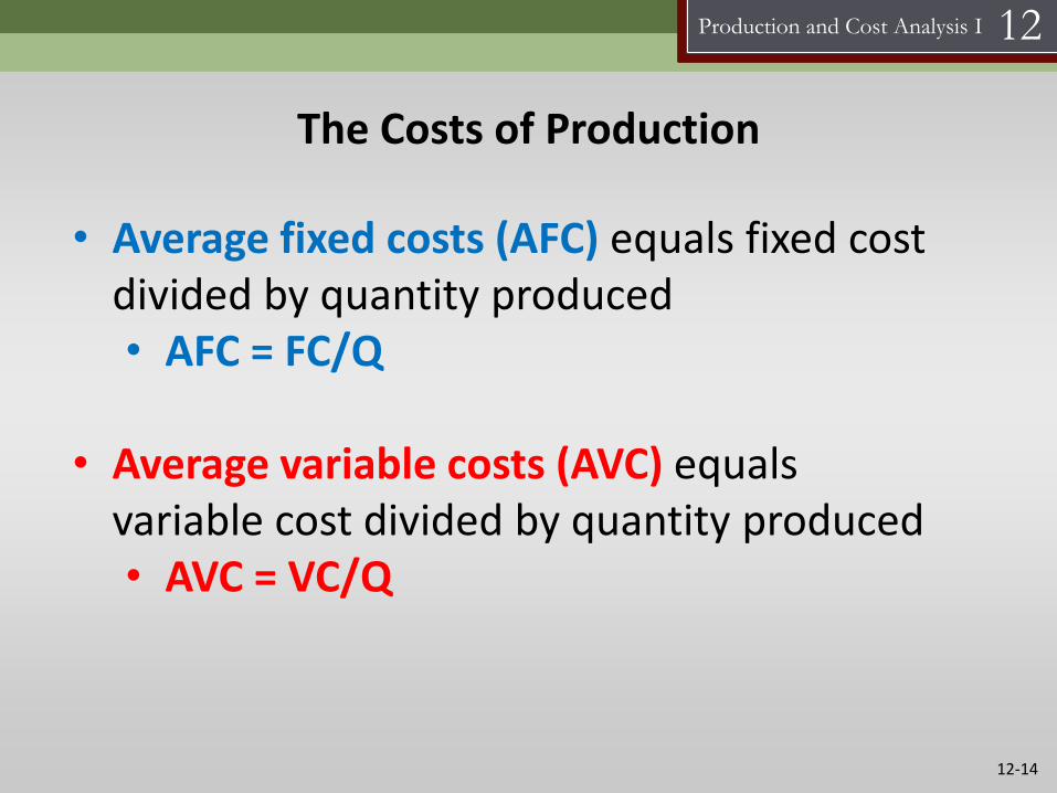
The Costs of Production
• Average fixed costs (AFC) equals fixed cost divided by quantity produced• AFC = FC/Q
• Average variable costs (AVC) equals variable cost divided by quantity produced• AVC = VC/Q
12-14

Production and Cost Analysis I 12
The Costs of Production
• Average total cost (ATC) equals total cost divided by quantity produced
• ATC = TC/Q or ATC = AFC + AVC
• Marginal cost (MC) is the increase in total cost when output increases by one unit
• MC = ΔTC/ΔQ
McGraw-Hill/Irwin Colander, Economics 15

Production and Cost Analysis I 12
Costs of Production Table
Output FC ($) VC ($) TC ($) MC ($) AFC ($) AVC ($) ATC ($)
3 50 38 8812
16.67 12.66 29.33
4 50 50 100 12.50 12.50 25.00
9 50 100 1508
5.56 11.11 16.67
10 50 108 158 5.00 10.80 15.80
16 50 150 2007
3.13 9.38 12.51
17 50 157 207 2.94 9.24 12.18
22 50 200 25010
2.27 9.09 11.36
23 50 210 260 2.17 9.13 11.30
27 50 255 30515
1.85 9.44 11.29
28 50 270 320 1.79 9.64 11.43
32 50 400 450 1.56 12.50 14.06
12-16

Production and Cost Analysis I 12
The Shapes of Cost Curves
• The variable and total cost curves have the same shape
• Increasing output increases VC and TC
• The fixed cost curve is always constant
• Increasing output doesn’t change FC
12-17

Production and Cost Analysis I 12
Graphing Total Cost Curves
FC
Total Cost
FC curve is constant
TC and VC curves
increase as Q increases
Q
500
400
300
200
100
04 8 12 16 20 24 28 32
VC
TC
12-18

Production and Cost Analysis I 12
The Shapes of Cost Curves
• The average fixed cost (AFC) curve is downward sloping
• Increasing output decreases AFC
• The marginal cost (MC), average variable cost (AVC), and average total cost curves (ATC) are U-shaped
• Increasing output initially leads to a decrease in MC, AVC, and ATC but eventually they increase
McGraw-Hill/Irwin Colander, Economics 19

Production and Cost Analysis I 12
Graphing Per Unit Output Cost Curves
AVC
MC
ATC
AFCQ
Cost
AFC curve decreases
MC, ATC, and AVC curves
are U-shaped
35
30
25
20
15
10
5
04 8 12 16 20 24 28 32
12-20

Production and Cost Analysis I 12
The Shapes of Cost Curves
• The marginal cost curve goes through the minimum points of the ATC and AVC curves (remember this)
McGraw-Hill/Irwin Colander, Economics 21

Production and Cost Analysis I 12
Draw the Graph: Marginal Cost, AVC, and ATC
AVC
MC
Q
Costs per unit
ATCThe marginal cost curve goes through the minimum point
of both the ATC and AVC curves
12-22

Production and Cost Analysis I 12
• If MC > ATC, then ATC is rising
• If MC > AVC, then AVC is rising
• If MC < ATC, then ATC is falling
• If MC < AVC, then AVC is falling
• If MC = AVC and MC = ATC, then AVC and ATC are at their minimum points
The Relationship Between Marginal Cost and Average Cost
12-23

Production and Cost Analysis I 12
Profit Maximization Using Total Revenue and Total Cost (CH 14; Not in your notes)
• Total Revenue= Price x Quantity
• Total revenue and total cost curves can be used to determine the profit-maximizing level of output
• Total cost is the cumulative sum of the marginal costs, plus the fixed costs
• Total profit is the difference between total revenue and total cost curves
14-24

Production and Cost Analysis I 12
Total Revenue and Total Cost Table(CH 14; Not in your notes)
Q Total Revenue ($) Total Cost ($) Total Profit ($)
0 0 40 -40
1 35 68 -33
2 70 88 -18
3 105 104 1
4 140 118 22
5 175 130 45
6 210 147 63
7 245 169 76
8 280 199 81
9 315 239 76
10 350 293 57
Total profit is maximized at 8 units
of output
14-25

Production and Cost Analysis I 12
Total Revenue and Total Cost Table (CH 14; Not in your notes)
Total Cost, Total Revenue
TC
$175
Q
$130
$280
85
TRThe total revenue curve is a
straight line
The total cost curve is bowed upward at most
quantities reflecting increasing marginal cost
Could see this graph in the multiple choice
3
Losses LossesProfits
Profits are maximized when the vertical distance
between TR and TC is greatest
14-26

Production and Cost Analysis I 12
Chapter Summary
• Accounting profit is explicit revenue less explicit cost
• Economists include implicit revenue and cost in determining
economic profit
• Implicit revenue includes the increases in the value of assets
owned by the firm
• Implicit costs include opportunity cost of time and capital
provided by owners of the firm
• In the long run a firm can choose among all possible
production techniques; in the short run it is constrained in
its choices because at least one input is fixed
12-27

Production and Cost Analysis I 12
Chapter Summary
• The law of diminishing marginal productivity states that as more
of a variable input is added to a fixed input, the additional
output will eventually be decreasing
• Costs are generally divided into fixed costs, variable costs, and
marginal costs
• TC = FC + VC
• MC = ΔTC/ΔQ
• AFC = FC/Q
• AVC = VC/Q
• ATC = AFC + AVC
12-28

Production and Cost Analysis I 12
Chapter Summary
• The law of diminishing marginal productivity causes marginal
and average costs to rise
• MC goes through the minimum points of the AVC and ATC
• If MC > ATC, then ATC is rising
• If MC = ATC, then ATC is constant
• If MC < ATC, then ATC is falling
12-29

Production and Cost Analysis II 13
Production and Cost Analysis II
Economic efficiency consists of making
things that are worth more than they cost.
— J. M. Clark
CHAPTER 13
Copyright © 2010 by the McGraw-Hill Companies, Inc. All rights reserved.McGraw-Hill/Irwin

Production and Cost Analysis II 13
Technical Efficiency and Economic Efficiency
• Technical efficiency in production means that as few inputs as possible are used to produce a given output
• The economically efficient method of production produces a given level of output at the lowest possible cost
13-31

Production and Cost Analysis II 13
Shape of the Long run ATC
• The law of diminishing marginal productivity does not apply in the long run since all inputs are variable
• The shape of the long-run cost curve is due to the existence of economies and diseconomies of scale
13-32

Production and Cost Analysis II 13
Economies of Scale
• Economies of scale exist when long-run average total costs decrease as output increases
• These are shown by the downward sloping portion of the long-run ATC
13-33

Production and Cost Analysis II 13
Economies of Scale
• The minimum efficient level of production is the amount of production that spreads setup costs out sufficiently for firms to undertake production profitably
• This is where average total costs are at a minimum
13-34

Production and Cost Analysis II 13
Diseconomies of Scale
• Diseconomies of scale exist when long-run average total costs increase as output increases
• These are shown by the upward sloping portion of the long-run average total cost curve
13-35

Production and Cost Analysis II 13
A Typical Long run Average Total Cost Curve
Q
Costs per unit
11
$50
$55
17
$60
14 20
Long-run average total cost (LRATC)
Economies of scale Constant returns to scale
Diseconomies of scale
Minimum efficient level
of production
13-36

Production and Cost Analysis II 13
Constant Returns to Scale
• Constant returns to scale exist when average total costs do not change as output increases
• This is shown by the flat portion of the long-run average total cost curve
• Constant returns to scale occur when production techniques can be replicated again and again to increase output
13-37

Production and Cost Analysis II 13
A Typical Long run ATC Table
QTC of Labor
($)
TC of Machines
($)TC ($) ATC ($)
11 381 254 635 58
12 390 260 650 54
13 402 268 670 52
14 420 280 700 50
15 450 300 750 50
16 480 320 800 50
17 510 340 850 50
18 549 366 915 51
19 600 400 1000 53
20 666 444 1110 56
ATC falls because of economies of
scale
ATC is constant because of
constant returns to scale
ATC rises because of
diseconomies of scale
13-38

Production and Cost Analysis II 13
Chapter Summary
• An economically efficient production process must be technically efficient, but a technically efficient process may not be economically efficient
• The long-run average total cost curve is U-shaped because economies of scale cause average total cost to decrease; diseconomies of scale eventually cause average total cost to increase
• Marginal cost and short-run average cost curves slope upward because of diminishing marginal productivity
13-39

Production and Cost Analysis II 13
Chapter Summary
• The long-run average cost curve slopes upward because of diseconomies of scale
• Costs in the real world are affected by:
• Economies of scope
• Learning by doing and technological change
• Many dimensions to output
• Unmeasured costs, such as opportunity costs
13-40