Embed Size (px)
Citation preview
arX
iv:1
408.
1361
v1 [
phys
ics.
soc-
ph]
6 A
ug 2
014
Maximizing a psychological uplift in lovedynamics
Malay Banerjee, Anirban Chakraborti and Jun-ichi Inoue
Abstract In this paper, we investigate the dynamical properties of a psychologicaluplift in lovers. We first evaluate extensively the dynamical equations which were re-cently given by Rinaldiet. al.(2013) [1]. Then, the dependences of the equations onseveral parameters are numerically examined. From the viewpoint of lasting part-nership for lovers, especially, for married couples, one should optimize the param-eters appearing in the dynamical equations to maintain the love for their respectivepartners. To achieve this optimization, we propose a new idea where the parametersare stochastic variables and the parameters in the next timestep are given as expec-tations over a Boltzmann-Gibbs distribution at a finite temperature. This idea is verygeneral and might be applicable to other models dealing withhuman relationships.
1 Introduction
“Love is composed of a single soul inhabiting two bodies.” – Aristotle
“Love never dies a natural death. It dies because we don’t know how to replenish its source.It dies of blindness and errors and betrayals. It dies of illness and wounds; it dies of weari-ness, of witherings, of tarnishings.” – Anaı̈s Nin
Love – mysterious and unexplained – often forms the basis of arelationshipbetween two persons; undoubtedly, a partnership between lovers is a time-dependent
Malay BanerjeeDepartment of Mathematics and Statistics, Indian Institute of Technology, Kanpur-208016, INDIAe-mail:[email protected]
Anirban ChakrabortiSchool of Computational and Integrative Sciences, Jawaharlal Nehru University, New Delhi-110067, INDIA e-mail:[email protected]
Jun-ichi InoueGraduate School of Information Science and Technology, Hokkaido University, N14-W9, Kita-ku,Sapporo 060-0814, JAPAN e-mail:[email protected]
1
2 Malay Banerjee, Anirban Chakraborti and Jun-ichi Inoue
phenomenon. Even if a man and a woman were in deep love at some initial stages,the psychological uplift for one or both of them could eventually decay to very low-levels, and could even result in a break-up or divorce, in theworst scenario.
A simple mathematical model for the dynamics of love betweena man andwoman was introduced by Strogatz [2, 3] – the first attempt to model the love dy-namics with the help of coupled ordinary differential equations. The idea of Stro-gatz was then extended by other researchers [4, 5, 6] to understand the influenceof the factors like appeal, secure relation between the couple, separation for a finitetime period, which are important factors to maintain the relationship. Similar typeof mathematical models have been proposed and analyzed up tocertain extent fortriangular love by Sprott [7, 8] but the uncertainty for the final outcome remainsunclear. Recently, Rinaldiet. al. [1] again proposed a simple dynamical model forlovers emotion to investigate a law of big hit film from the dynamical behavior offeeling in the partner for lovers. Their approach, based on acoupled differentialequations, was applied to the movie ‘Gone With The Wind’ (GWTW); they foundthat the resulting time series of lovers’ feelings can mimicthe story of the film tosome extent. The differential equations contain several parameters and Rinaldiet.al. chose them to mimic the lives of Scarlet and Rhett, with full of ups and downs. Inthe romantic film GWTW, the drastic ups and downs in the lovers’ emotions indeedconstituted a notable factor to attract the attention of audience and the sequences ofsuch psychological climaxes in the film might have been a key issue in making thefilm a big hit, as suggested by Rinaldiet. al.(2013) [1].
In reality, for a married couple, such extreme ups and downs could however proveto be deterrent to the continuation a peaceful married life.Hence, from the viewpoint of lasting partnership for lovers, especially for a married couple, one shouldoptimize the parameters appearing in the dynamical equations to maintain the lovefor their partner. In other words, it would be interesting toobtain the optimum levelsof the parameters in order to maintain the minimum level of love and happinessrequired to maintain a happy and prolonged marital life.
To this aim, we propose a simple new idea in this paper. We assume that theparameters involved with the love dynamics are not constantover the entire timeperiod, rather they are stochastic variables and the parameters in the next time stepare given as expectations over a Boltzmann-Gibbs distribution at a finite tempera-ture. By decreasing the temperature during the dynamics of coupled equations, onecan accelerate the rate of increase of the sum of feelings (and decrease the differ-ence of feelings) of lovers at each time step. The idea is quite general and might beapplicable to other models dealing with human relationships.
2 Differential equations of gross and gap for lovers’ feelings
In the original model by Rinaldiet. al. [1], the governing equations with respectto the feelings of lovers, denoted asx1,x2, are given by two coupled non-linearordinary differential equations:
Maximizing a psychological uplift in love dynamics 3
dx1
dt= −α1x1+ρ1A2+ k1x2e−η1x2, (1)
dx2
dt= −α2x2+ρ2A1+ k2x1e−η2x1, (2)
subjected to the positive initial conditions, where the parameterαi is forgetting co-efficient, ki andηi are the parameters characterizing the measure of insecurity feel-ings,A j is the measure of appeal towardsxi produced byx j andρi is a multiplicativefactor representing the amount of recognition of the appealA j (see [1] for detailedinterpretation). All the parameters involved with the model are positive. Interest-ingly, once we choose the initial values ofx1,x2, these variables remain positive.
As one can see above, that there are many parameters to be calibrated. From theengineering point of view, one could determine them by meansof ‘optimization’of some appropriate cost functions. In the following, we consider several such costfunctions.
First, we introduce the following new variables, namely, the ‘gross’S (sum) and‘gap’ D (difference):
S≡ x1+ x2, D ≡ (x1− x2)2 = x2
1+ x22−2x1x2. (3)
This allows us to write:
x1 =12(S+
√D), x2 =
12(S−
√D), (4)
where we should bear in mind that we have to consider the casex1 ≥ x2 in orderto have the well-defined expressions forx1 andx2 in terms ofS andD. Of course,this condition may not always be satisfied. However, as we arefocusing here on thegapD, the above choice might be indeed justified. It should be noted that the grossfeelingsS could be regarded as a cost function to be maximized. This is becausethe total degree of ‘passion’ amongst the lovers might be oneof the most importantquantities to make the relationship strong and durable. On the other hand, the gapthe two partners’ lovex1,x2 might determine the ‘stability’ of the relationship –namely, even if theS is high, the mutual relation could be unstable whenx1 ≫ x2
or x1 ≪ x2. In other words, it is very hard for the lovers to continue their goodrelationship if only one of them expresses too much love to his/her love partner andthe other partner becomes indifferent about their relationship which was establisheddue to their love affairs. Two hypothetical cases can be considered for illustratingthis.
• For young lovers, the variableS takes high values temporally; however, one per-son (girl or boy) suddenly loses interest and becomes indifferent. As a result, thevariableD increases rapidly and the love affair (marriage) breaks down prema-turely.
• For senior lovers, the variableS normally does not take a high value; however,they know each other quite well, and as a result, the feelingsx1 andx2 are quite
4 Malay Banerjee, Anirban Chakraborti and Jun-ichi Inoue
similar. Hence, variableD increases and the love affair (marriage) becomes sta-ble.
We do not have any real survey data to validate these idealized examples. Never-theless, we consider an utility functionS, which is to be maximized, and the energyfunctionD, which is to be minimized, in order to determine the parameters appear-ing in the original model [1].
Then, the original equations are rewritten in terms ofSandD. The equation forS is easy to obtain, and we have
dSdt
= −α1S+
√D
2+ρ1A2+ k1
S−√
D2
e−η1(S−√
D)/2−α2S−
√D
2
+ ρ2A1+ k2S+
√D
2e−η2(S+
√D)/2 ≡ f (θθθ : S,D) (5)
dDdt
= 2(x1− x2)
(
dx1
dt− dx2
dt
)
≡ g(θθθ : S,D), (6)
whereθθθ ≡ (α1,α2,ρ1,ρ2,A2,A2,k1,k2,η1,η2).In the following parts, we discuss in details, the behavior of the non-linear dy-
namics of equations (5)-(6), within the framework of Rinaldi et. al. [1] model, andconsider the possible optimization of the parameters. Here, we have chosen themodel by Rinaldiet. al. just as a basic example, and in principle one could eas-ily extend the study by taking into account much more complicated and appropriatelovers’ interactions.
2.1 Some specific choices of parameters
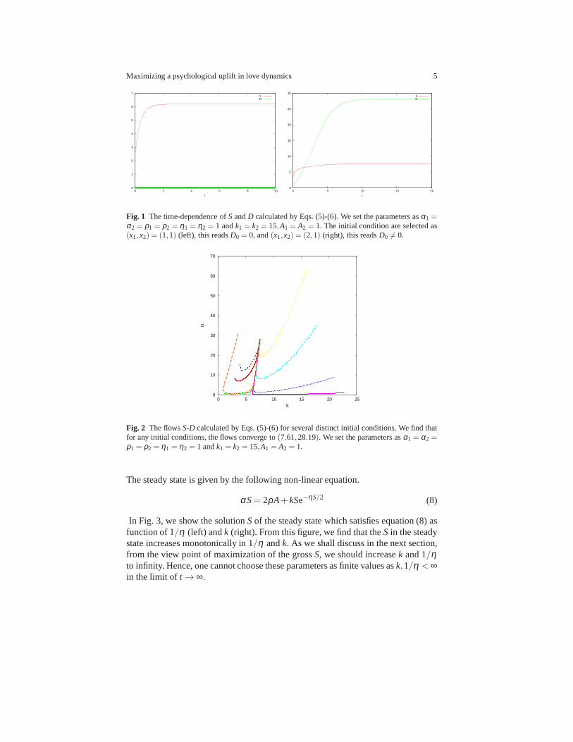
We first examine the behavior of the differential equations (5) and (6) with respectto S andD for the case of a specific choice of parametersθθθ . Apparently,Dt = 0is always a solution of the equation (6). In Fig. 1, we plot theSt andDt for twodistinct initial conditions. In the left panel, we choose the initial condition so thatx1(0)= x2(0) = 1, this readsD0 = 0. From this panel, we easily find that the gapD istime-independently zero. On the other hand, in the right panel, we choose asx1(0) 6=x2(0), namely,D0 6= 0. For this case, the gapD evolves in time and converges tosome finite value. In Fig. 2, we show the flows (trajectories)S-D for D0 6= 0. Allflows converge to(7.61,28.19).
2.1.1 Symmetric case
For symmetric caseDt = 0 (x1 = x2), the differential equation with respect toS issimply obtained by
dSdt
=−αS+2ρA+ kSe−ηS/2. (7)
Maximizing a psychological uplift in love dynamics 5
0
1
2
3
4
5
6
7
0 2 4 6 8 10
t
SD
0
5
10
15
20
25
30
0 5 10 15 20
t
SD
Fig. 1 The time-dependence ofSandD calculated by Eqs. (5)-(6). We set the parameters asα1 =α2 = ρ1 = ρ2 = η1 = η2 = 1 andk1 = k2 = 15,A1 = A2 = 1. The initial condition are selected as(x1,x2) = (1,1) (left), this readsD0 = 0, and(x1,x2) = (2,1) (right), this readsD0 6= 0.
0
10
20
30
40
50
60
70
0 5 10 15 20 25
D
S
Fig. 2 The flowsS-D calculated by Eqs. (5)-(6) for several distinct initial conditions. We find thatfor any initial conditions, the flows converge to(7.61,28.19). We set the parameters asα1 = α2 =ρ1 = ρ2 = η1 = η2 = 1 andk1 = k2 = 15,A1 = A2 = 1.
The steady state is given by the following non-linear equation.
αS= 2ρA+ kSe−ηS/2 (8)
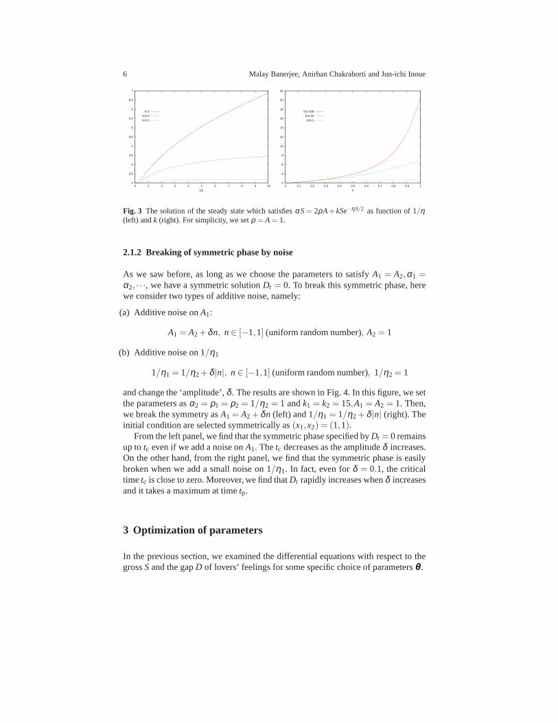
In Fig. 3, we show the solutionSof the steady state which satisfies equation (8) asfunction of 1/η (left) andk (right). From this figure, we find that theS in the steadystate increases monotonically in 1/η andk. As we shall discuss in the next section,from the view point of maximization of the grossS, we should increasek and 1/ηto infinity. Hence, one cannot choose these parameters as finite values ask,1/η < ∞in the limit of t → ∞.
6 Malay Banerjee, Anirban Chakraborti and Jun-ichi Inoue
2
2.5
3
3.5
4
4.5
5
5.5
6
6.5
7
0 1 2 3 4 5 6 7 8 9 10
1/η
k=1
k=0.5
k=0.1
2
4
6
8
10
12
14
16
18
20
22
0 0.1 0.2 0.3 0.4 0.5 0.6 0.7 0.8 0.9 1
k
1/η=100
1/η=10
1/η=1
Fig. 3 The solution of the steady state which satisfiesαS= 2ρA+ kSe−ηS/2 as function of 1/η(left) andk (right). For simplicity, we setρ = A= 1.
2.1.2 Breaking of symmetric phase by noise
As we saw before, as long as we choose the parameters to satisfy A1 = A2,α1 =α2, · · ·, we have a symmetric solutionDt = 0. To break this symmetric phase, herewe consider two types of additive noise, namely:
(a) Additive noise onA1:
A1 = A2+ δn, n∈ [−1,1] (uniform random number), A2 = 1
(b) Additive noise on 1/η1
1/η1 = 1/η2+ δ |n|, n∈ [−1,1] (uniform random number), 1/η2 = 1
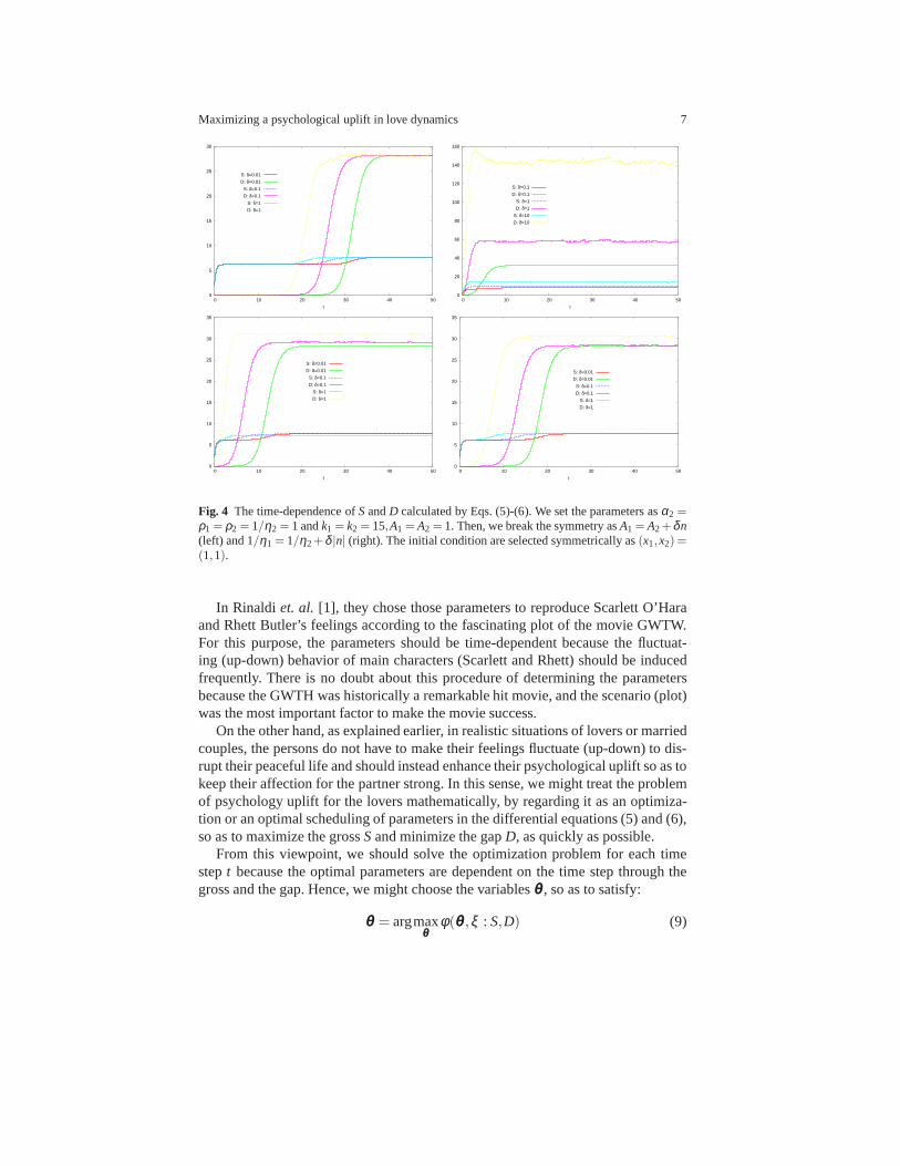
and change the ‘amplitude’,δ . The results are shown in Fig. 4. In this figure, we setthe parameters asα2 = ρ1 = ρ2 = 1/η2 = 1 andk1 = k2 = 15,A1 = A2 = 1. Then,we break the symmetry asA1 = A2+ δn (left) and 1/η1 = 1/η2+ δ |n| (right). Theinitial condition are selected symmetrically as(x1,x2) = (1,1).
From the left panel, we find that the symmetric phase specifiedby Dt = 0 remainsup totc even if we add a noise onA1. Thetc decreases as the amplitudeδ increases.On the other hand, from the right panel, we find that the symmetric phase is easilybroken when we add a small noise on 1/η1. In fact, even forδ = 0.1, the criticaltimetc is close to zero. Moreover, we find thatDt rapidly increases whenδ increasesand it takes a maximum at timetp.
3 Optimization of parameters
In the previous section, we examined the differential equations with respect to thegrossSand the gapD of lovers’ feelings for some specific choice of parametersθθθ .
Maximizing a psychological uplift in love dynamics 7
0
5
10
15
20
25
30
0 10 20 30 40 50
t
S: δ=0.01
D: δ=0.01
S: δ=0.1
D: δ=0.1
S: δ=1
D: δ=1
0
20
40
60
80
100
120
140
160
0 10 20 30 40 50
t
S: δ=0.1
D: δ=0.1
S: δ=1
D: δ=1
S: δ=10
D: δ=10
0
5
10
15
20
25
30
35
0 10 20 30 40 50
t
S: δ=0.01
D: δ=0.01
S: δ=0.1
D: δ=0.1
S: δ=1
D: δ=1
0
5
10
15
20
25
30
35
0 10 20 30 40 50
t
S: δ=0.01
D: δ=0.01
S: δ=0.1
D: δ=0.1
S: δ=1
D: δ=1
Fig. 4 The time-dependence ofSandD calculated by Eqs. (5)-(6). We set the parameters asα2 =ρ1 = ρ2 = 1/η2 = 1 andk1 = k2 = 15,A1 = A2 = 1. Then, we break the symmetry asA1 = A2+δn(left) and 1/η1 = 1/η2+δ |n| (right). The initial condition are selected symmetricallyas(x1,x2) =(1,1).
In Rinaldi et. al. [1], they chose those parameters to reproduce Scarlett O’Haraand Rhett Butler’s feelings according to the fascinating plot of the movie GWTW.For this purpose, the parameters should be time-dependent because the fluctuat-ing (up-down) behavior of main characters (Scarlett and Rhett) should be inducedfrequently. There is no doubt about this procedure of determining the parametersbecause the GWTH was historically a remarkable hit movie, and the scenario (plot)was the most important factor to make the movie success.
On the other hand, as explained earlier, in realistic situations of lovers or marriedcouples, the persons do not have to make their feelings fluctuate (up-down) to dis-rupt their peaceful life and should instead enhance their psychological uplift so as tokeep their affection for the partner strong. In this sense, we might treat the problemof psychology uplift for the lovers mathematically, by regarding it as an optimiza-tion or an optimal scheduling of parameters in the differential equations (5) and (6),so as to maximize the grossSand minimize the gapD, as quickly as possible.
From this viewpoint, we should solve the optimization problem for each timestept because the optimal parameters are dependent on the time step through thegross and the gap. Hence, we might choose the variablesθθθ , so as to satisfy:
θθθ = argmaxθθθ
φ(θθθ ,ξ : S,D) (9)
8 Malay Banerjee, Anirban Chakraborti and Jun-ichi Inoue
for each time step, where we defined the following utility function:
φ(θθθ ,ξ : S,D)≡ f (θθθ : S,D)− ξ g(θθθ : S,D) (10)
for ξ ≥ 0. The maximization given by equation (9) means that we accelerate thespeed of increasedS/dt(= f ) and−dD/dt(=−g) as much as possible during thedynamics ofSandD. Hence, when we choose the variableSfor the case ofξ = 0 tobe maximized for lovers, we should optimize the parameters appearing in the func-tion f . For each time step, the landscape off changes due to the dynamics ofD andS, and one should choose the solution, say,θθθ = (α1,α2, · · ·) so as to maximize thefunction f at each time step. As the result, we obtain the trajectory in the parameterspace:(α1(0),α2(0), · · ·)→ (α1(1),α2(1), · · ·)→ ···.
3.1 ‘Hard’ and ‘soft’ optimizations by using a concept of physics
In the following, for simplicity, we only consider the case of ξ = 0 and we alsocarry out the maximization of the speed of increasedS/dt (see equation (5) and donot take into account the maximization of−dD/dt (see equation (6)).
To achieve the parameter choice by means of physics, we startour argument fromthe following energy function:
E(θθθ : St ,Dt)≡− f (θθθ : St ,Dt). (11)
Obviously, in terms off , we should maximizef as a utility function. We shouldkeep in mind that we use the definition ofSt ,Dt instead ofS,D to recall us thatf istime dependent through those variables. We should bear in mind that the functionfis defined at each time stept. In this sense,f is just a function of only parametersα1,2, etc. to be selected at each time step. Therefore, the functionf is definitelyconserved at each timet.
From the viewpoint of ‘hard optimization’, we might utilizethe following gradi-ent descent learning for the parametersθθθ as
dθθθdt
=−∂E∂θθθ
=+∂ f∂θθθ
(12)
Obviously, the cost function for each time step is dependenton the state(St ,Dt). Aswe mentioned in the previous section (see Fig. 4),St ,Dt might contain some noiseand through the fluctuation inSt ,Dt , the parametersθθθ fluctuate around the peak ofthe locally concave functionf . To determine the parameters, we temporarily assumehere that the parameters are all ‘stochastic’ variables. Namely, to adapt ourselves tosuch realistic cases, we consider ensemble of the parameters and we carry out thefollowing maximization of Shannon’s entropy under the usual two constraints ofenergy conservation and probability conservation:
Maximizing a psychological uplift in love dynamics 9
H =−∫
dθθθP(θθθ) logP(θθθ)+β(
E−∫
dθθθE(θθθ : St ,Dt)P(θθθ ))
+λ(
1−∫
dθθθP(θθθ))
(13)whereβ ,λ are Lagrange multipliers. By making use of derivative with respect toP(θθθ),λ , we have
P(θθθ) =exp(β f (θθθ : St ,Dt))
∫
dθθθ exp(β f (θθθ : St ,Dt))(14)
This is nothing but the Boltzmann-Gibbs distribution with temperatureT = β−1.To obtain the appropriate parameters, we construct the following iterations:
θθθ (t+1) =
∫
dθθθP(θθθ) =∫
dθθθ θθθ exp(β f (θθθ : St ,Dt))∫
dθθθ exp(β f (θθθ : St ,Dt))(15)
We should keep in mind that the strict maximization off is achieved by taking thelimit of β → ∞. Namely, the solution for ‘hard optimization’ is recoveredas
θθθ (t+1)hard = lim
β→∞
∫
dθθθ θθθ exp(β f (θθθ : St ,Dt))∫
dθθθ exp(β f (θθθ : St ,Dt)). (16)
These types of adaptive learning procedure have been well known since the refer-ence [9] in the literature of neural networks.
It is important for us to obtain the strict solution, of course. Hoowever, here weconsider only the case ofβ = 1, since we are dealing with the situation in which theparametersθθθ are not deterministic variables; rather, stochastic variables fluctuatingaround the peaks off .
From the view point of optimization, note that the functionf is not locally ‘con-cave’ for any choice ofSt ,Dt . Hence, the parametersθθθ which should be selectedare trivially going to their ‘bounds’. Nevertheless in the following, we derive theconcrete update rule for each parameter. We first consider the parameterα1. Here,we assume thatα1,2 take any value in[0,∞). Hence, we obtain
α(t+1)1 =
∫ ∞0 dα1α1e−α1(St+
√Dt )/2
∫ ∞0 dα1e−α1(St+
√Dt )/2
=2
St +√
Dt, α(t+1)
2 =2
St −√
Dt. (17)
Hence, we find that the parametersα1,2 decrease as inverse of the dynamicsSt tozero, when we consider the symmetric caseDt = 0. Therefore, as we expected,α1,2 go to the boundα1,2 = 0 but the optimal scheduling, namely, the speed ofconvergence to the boundα1,2 ∼ 1/St is not trivial and would be worthwhile for usto investigate extensively.
We next considerρ1,2. For simplicity, we assume that these two parameters takevalues in[0,1]. After simple algebra, we have
ρ (t+1)1 =
∫ 10 dρ1ρ1eA2ρ1
∫ 10 dρ1eA2ρ1
=A(t)
2 eA(t)2 −eA
(t)2 +1
A(t)2 (eA
(t)2 −1)
, ρ (t+1)2 =
A(t)1 eA
(t)1 −eA
(t)1 +1
A(t)1 (eA
(t)1 −1)
. (18)
10 Malay Banerjee, Anirban Chakraborti and Jun-ichi Inoue
Sinceρ andA are ‘conjugates’ in the argument of the exponential, we immediatelyhave
A(t+1)1 =
ρ (t)2 eρ(t)
2 −eρ(t)2 +1
ρ (t)2 (eρ(t)
2 −1), A(t+1)
2 =ρ (t)
1 eρ(t)1 −eρ(t)
1 +1
ρ (t)1 (eρ(t)
1 −1). (19)
Fork1,2, the structures are exactly similar to those ofA andρ , when we assume thatk1,2 ∈ [0,1]. We easily obtain
k(t+1)1 =
Q(t)1 eQ
(t)1 −eQ
(t)1 +1
Q(t)1 (eQ
(t)1 −1)
, Q(t)1 ≡ (St −
√Dt)
2e−η(t)
1 (St−√
Dt )/2, (20)
k(t+1)2 =
Q(t)2 eQ
(t)2 −eQ
(t)2 +1
Q(t)2 (eQ(t)
2 −1), Q(t)
2 ≡ (St +√
Dt)
2e−η(t)
2 (St+√
Dt )/2. (21)
Finally, we considerη1,2. Here we also assume thatη1,2 ∈ [0,∞). Then, we can write
η(t+1)1 =
∫ ∞0 dη1η1exp[ k(t)(St−
√Dt )
2 e−η1(St−√
Dt )/2]∫ ∞
0 dη1exp[ k(t)(St−√
Dt )2 e−η1(St−
√Dt )/2]
(22)
η(t+1)2 =
∫ ∞0 dη2η2exp[ k(t)(St+
√Dt )
2 e−η2(St+√
Dt )/2]∫ ∞
0 dη2exp[ k(t)(St−√
Dt )2 e−η1(St−
√Dt )/2]
(23)
Carrying out the above procedure, one could only ‘soft’ (not‘hard’) optimize thequantityS. By substituting the results into the differential equation with respect toD (see equation (6)) at the same time, we may obtain the behavior of the gap.
4 Discussions and remarks
In this paper, we first introduced the Rinaldi model and the framework to discusssome kind of optimality of a person’s behavior, in terms of optimization in themathematical sense. For this, we have just formulated the acceleration rate of thegrossdS/dt, namely, the right hand side of equation (5), the functionf , at eachtime step. However, the functionf is not locally concave and the value of optimalparameters go either to zero or to infinity, ast → ∞. Nevertheless, we can still dis-cuss the scheduling of parameters. For instance, the parametersα1,2 should decayas∼ S−1
t when we attempt to maximize thef from the viewpoint of ‘soft optimiza-tion’. In near future, we would like to consider and discuss the result of optimizationextensively, by considering the validity of the model itself.
Here, we have setβ = 1 in the calculations. However, we can always regardβ asa time dependent parameter– the ‘inverse-temperature’, appearing in the context of‘simulated annealing’, and defined by
Maximizing a psychological uplift in love dynamics 11
Tt = β−1t =
c1
(t + c2)ζ (log(t + c3))ε (24)
where the coefficientsc1,2,3,ζ ,ε determine the speed of convergence. As we alreadymentioned, the utility functionf changes through the dynamical variablesSt ,Dt .Hence, the utility surface also evolves in time. In the abovescheduling, we have alsoassumed that the temperate is decreasing within the same time scale as dynamicalvariablesSt ,Dt and parametersθθθ . However, we can also consider the case in whichT is scheduled in much shorter time scale thanSt ,Dt and in the same time scaleasθθθ , namely,Tτ ,θθθ τ with τ ≪ t. Then, the procedure defined by equation (16) isregarded as the “deterministic annealing” [10]. In such a general case, the optimalscheduling for the parametersθθθ might be changed and extensive study along thisdirection will be reported in our forthcoming paper.
A few other specific remarks are mentioned below:
1. In the model considered here, the parameters values are the same as those ofRinaldi et. al. [1], but this choice is neither unique nor true for all the “realis-tic” situations. A thorough study with other choices of parameters is very muchnecessary.
2. Identification of the most sensitive parameters responsible for the long time sur-vival of the relationship remains an interesting and open problem. Such identi-fication and then introduction of stochastic fluctuations atthe limiting situationscould certainly provide more insight towards the modellingapproach.
3. The present work is sort of a preliminary attempt of understanding the love dy-namics – theory for the case of sustainability of the love relation between a cou-ple. In reality, the dynamics of love affairs and related modelling approach needmore careful and thorough investigations; the effects of several factors have notbeen considered so far, for example, how the presence of one or more competingperson(s) along with the couple, who are in a love relation toeach other, caninfluence the dynamics. Along the lines of the triangular love studies by Sprott[7, 8], it might be very interesting to investigate the role of SandD, in order todetermine the steady-state relationship between a couple for the case of triangularlove. Amongst many other interesting questions, one could also investigate howdoes a period of separation affect the system dynamics, within this modellingapproach.
Acknowledgements One of the authors (JI) was financially supported by Grant-in-Aid for Scien-tific Research (C) of Japan Society for the Promotion of Science (JSPS) No. 2533027803, Grant-in-Aid for Scientific Research (B) No. 26282089, and Grant-in-Aid for Scientific Research onInnovative Area No. 2512001313.
References
1. S. Rinaldi, F. Della Rossa and P. Landi,Physica A392, pp. 3231-3239 (2013).2. S. H. Strogatz,Math. Mag.61, pp. 35 (1998).

12 Malay Banerjee, Anirban Chakraborti and Jun-ichi Inoue
3. S. H. Strogatz,Nonlinear Dynamics And Chaos: With Applications To Physics, Biology, Chem-istry, And Engineering(Westview Press, 1994).
4. A. Gragnani, S. Rinaldi, G. Feichtinger,Int. J. Bifur. Chaos7, pp. 2611-2699 (1997).5. S. Rinaldi,Appl. Math. Comput.95, pp. 181-192 (1998).6. S. Rinaldi, A. Gragnani,Nonlin. Dyn. Psych. Life Sci.2, pp. 298-301 (1998).7. J.C. Sprott,Nonlin. Dyn. Psych. Life Sci.8, pp. 303-314 (2004).8. J.C. Sprott,Nonlin. Dyn. Psych. Life Sci.9, pp. 23-36 (2005).9. S. Amari,IEEE Transactions on Electronic ComputersEC-16, NO. 3, pp. 299-307 (1967).
10. E. Levin, N. Tishby and S. Solla,Proceedings of the IEEE78, NO. 10, OCTOBER, pp.1568-1574 (1990).