Embed Size (px)
Citation preview
Week 3Matrix-Vector Operations
3.1 Opening Remarks
3.1.1 Timmy Two Space
* View at edX
Homework 3.1.1.1 Click on the below link to open a browser window with the “Timmy Two Space” exercise.This exercise was suggested to us by our colleague Prof. Alan Cline. It was first implemented using an IPythonNotebook by Ben Holder. During the Spring 2014 offering of LAFF on the edX platform, one of the partici-pants, Ed McCardell, rewrote the activity as * Timmy! on the web. (If this link does not work, openLAFF-2.0xM/Timmy/index.html).If you get really frustrated, here is a hint:
* View at edX
81

Week 3. Matrix-Vector Operations 82
3.1.2 Outline Week 3
3.1. Opening Remarks . . . . . . . . . . . . . . . . . . . . . . . . . . . . . . . . . . . . . . . . . . . . . . . . . 813.1.1. Timmy Two Space . . . . . . . . . . . . . . . . . . . . . . . . . . . . . . . . . . . . . . . . . . . . . 813.1.2. Outline Week 3 . . . . . . . . . . . . . . . . . . . . . . . . . . . . . . . . . . . . . . . . . . . . . . . 823.1.3. What You Will Learn . . . . . . . . . . . . . . . . . . . . . . . . . . . . . . . . . . . . . . . . . . . . 83
3.2. Special Matrices . . . . . . . . . . . . . . . . . . . . . . . . . . . . . . . . . . . . . . . . . . . . . . . . . . 843.2.1. The Zero Matrix . . . . . . . . . . . . . . . . . . . . . . . . . . . . . . . . . . . . . . . . . . . . . . 843.2.2. The Identity Matrix . . . . . . . . . . . . . . . . . . . . . . . . . . . . . . . . . . . . . . . . . . . . . 853.2.3. Diagonal Matrices . . . . . . . . . . . . . . . . . . . . . . . . . . . . . . . . . . . . . . . . . . . . . 883.2.4. Triangular Matrices . . . . . . . . . . . . . . . . . . . . . . . . . . . . . . . . . . . . . . . . . . . . . 913.2.5. Transpose Matrix . . . . . . . . . . . . . . . . . . . . . . . . . . . . . . . . . . . . . . . . . . . . . . 943.2.6. Symmetric Matrices . . . . . . . . . . . . . . . . . . . . . . . . . . . . . . . . . . . . . . . . . . . . 97
3.3. Operations with Matrices . . . . . . . . . . . . . . . . . . . . . . . . . . . . . . . . . . . . . . . . . . . . . 993.3.1. Scaling a Matrix . . . . . . . . . . . . . . . . . . . . . . . . . . . . . . . . . . . . . . . . . . . . . . 993.3.2. Adding Matrices . . . . . . . . . . . . . . . . . . . . . . . . . . . . . . . . . . . . . . . . . . . . . . 102
3.4. Matrix-Vector Multiplication Algorithms . . . . . . . . . . . . . . . . . . . . . . . . . . . . . . . . . . . . 1053.4.1. Via Dot Products . . . . . . . . . . . . . . . . . . . . . . . . . . . . . . . . . . . . . . . . . . . . . . 1053.4.2. Via AXPY Operations . . . . . . . . . . . . . . . . . . . . . . . . . . . . . . . . . . . . . . . . . . . . 1083.4.3. Compare and Contrast . . . . . . . . . . . . . . . . . . . . . . . . . . . . . . . . . . . . . . . . . . . 1103.4.4. Cost of Matrix-Vector Multiplication . . . . . . . . . . . . . . . . . . . . . . . . . . . . . . . . . . . 111
3.5. Wrap Up . . . . . . . . . . . . . . . . . . . . . . . . . . . . . . . . . . . . . . . . . . . . . . . . . . . . . . 1123.5.1. Homework . . . . . . . . . . . . . . . . . . . . . . . . . . . . . . . . . . . . . . . . . . . . . . . . . 1123.5.2. Summary . . . . . . . . . . . . . . . . . . . . . . . . . . . . . . . . . . . . . . . . . . . . . . . . . . 112
3.1. Opening Remarks 83
3.1.3 What You Will Learn
Upon completion of this unit, you should be able to
• Recognize matrix-vector multiplication as a linear combination of the columns of the matrix.
• Given a linear transformation, determine the matrix that represents it.
• Given a matrix, determine the linear transformation that it represents.
• Connect special linear transformations to special matrices.
• Identify special matrices such as the zero matrix, the identity matrix, diagonal matrices, triangular matrices, and sym-metric matrices.
• Transpose a matrix.
• Scale and add matrices.
• Exploit properties of special matrices.
• Extrapolate from concrete computation to algorithms for matrix-vector multiplication.
• Partition (slice and dice) matrices with and without special properties.
• Use partitioned matrices and vectors to represent algorithms for matrix-vector multiplication.
• Use partitioned matrices and vectors to represent algorithms in code.
Week 3. Matrix-Vector Operations 84
3.2 Special Matrices
3.2.1 The Zero Matrix
* View at edX
Homework 3.2.1.1 Let L0 : Rn→ Rm be the function defined for every x ∈ Rn as L0(x) = 0, where 0 denotes thezero vector “of appropriate size”. L0 is a linear transformation.
True/False
We will denote the matrix that represents L0 by 0, where we typically know what its row and column sizes are from context(in this case, 0 ∈ Rm×n). If it is not obvious, we may use a subscript (0m×n) to indicate its size, that is, m rows and n columns.
By the definition of a matrix, the jth column of matrix 0 is given by L0(e j) = 0 (a vector with m zero components). Thus,the matrix that represents L0, which we will call the zero matrix, is given by the m×n matrix
0 =
0 0 · · · 0
0 0 · · · 0...
.... . .
...
0 0 · · · 0
.
It is easy to check that for any x ∈ Rn, 0m×nxn = 0m.
Definition 3.1 A matrix A ∈ Rm×n equals the m×n zero matrix if all of its elements equal zero.
Througout this course, we will use the number 0 to indicate a scalar, vector, or matrix of “appropriate size”.
In Figure 3.1, we give an algorithm that, given an m× n matrix A, sets it to zero. Notice that it exposes columns one at atime, setting the exposed column to zero.
MATLAB provides the function “zeros” that returns a zero matrix of indicated size. Your are going to write your own, tohelps you understand the material.
Make sure that the path to the laff subdirectory is added in MATLAB, so that the various routines form the laff library thatwe are about to use will be found by MATLAB. How to do this was discussed in Unit 1.6.3.
Homework 3.2.1.2 With the FLAME API for MATLAB (FLAME@lab) implement the algorithm in Figure 3.1.You will use the function laff zerov( x ), which returns a zero vector of the same size and shape (column orrow) as input vector x. Since you are still getting used to programming with M-script and FLAME@lab, you maywant to follow the instructions in this video:
* View at edXSome links that will come in handy:
• * Spark(alternatively, open the file * LAFF-2.0xM/Spark/index.html)
• * PictureFLAME(alternatively, open the file * LAFF-2.0xM/PictureFLAME/PictureFLAME.html)
You will need these in many future exercises. Bookmark them!
3.2. Special Matrices 85
Algorithm: [A] := SET TO ZERO(A)
Partition A→(
AL AR
)whereAL has 0 columns
while n(AL)< n(A) do
Repartition(AL AR
)→(
A0 a1 A2
)wherea1 has 1 column
a1 := 0 (Set the current column to zero)
Continue with(AL AR
)←(
A0 a1 A2
)endwhile
Figure 3.1: Algorithm for setting matrix A to the zero matrix.
Homework 3.2.1.3 In the MATLAB Command Window, type
A = zeros( 5,4 )
What is the result?
Homework 3.2.1.4 Apply the zero matrix to Timmy Two Space. What happens?
1. Timmy shifts off the grid.
2. Timmy disappears into the origin.
3. Timmy becomes a line on the x-axis.
4. Timmy becomes a line on the y-axis.
5. Timmy doesn’t change at all.
3.2.2 The Identity Matrix
* View at edX
Homework 3.2.2.1 Let LI : Rn→Rn be the function defined for every x ∈Rn as LI(x) = x. LI is a linear transfor-mation.
True/False
We will denote the matrix that represents LI by the letter I (capital “I”) and call it the identity matrix. Usually, the size ofthe identity matrix is obvious from context. If not, we may use a subscript, In, to indicate the size, that is: a matrix that has nrows and n columns (and is hence a “square matrix”).
Week 3. Matrix-Vector Operations 86
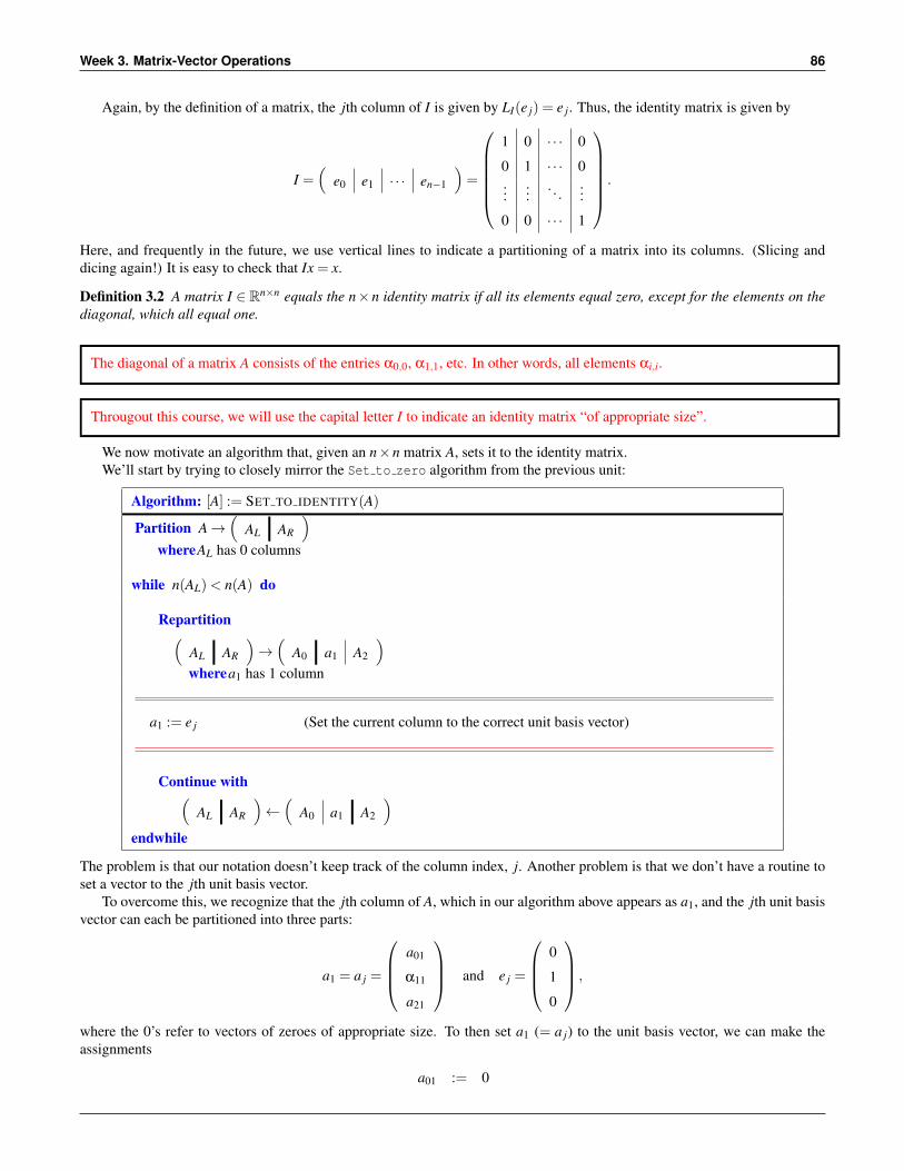
Again, by the definition of a matrix, the jth column of I is given by LI(e j) = e j. Thus, the identity matrix is given by
I =(
e0 e1 · · · en−1
)=
1 0 · · · 0
0 1 · · · 0...
.... . .
...
0 0 · · · 1
.
Here, and frequently in the future, we use vertical lines to indicate a partitioning of a matrix into its columns. (Slicing anddicing again!) It is easy to check that Ix = x.
Definition 3.2 A matrix I ∈ Rn×n equals the n×n identity matrix if all its elements equal zero, except for the elements on thediagonal, which all equal one.
The diagonal of a matrix A consists of the entries α0,0, α1,1, etc. In other words, all elements αi,i.
Througout this course, we will use the capital letter I to indicate an identity matrix “of appropriate size”.
We now motivate an algorithm that, given an n×n matrix A, sets it to the identity matrix.We’ll start by trying to closely mirror the Set to zero algorithm from the previous unit:
Algorithm: [A] := SET TO IDENTITY(A)
Partition A→(
AL AR
)whereAL has 0 columns
while n(AL)< n(A) do
Repartition(AL AR
)→(
A0 a1 A2
)wherea1 has 1 column
a1 := e j (Set the current column to the correct unit basis vector)
Continue with(AL AR
)←(
A0 a1 A2
)endwhile
The problem is that our notation doesn’t keep track of the column index, j. Another problem is that we don’t have a routine toset a vector to the jth unit basis vector.
To overcome this, we recognize that the jth column of A, which in our algorithm above appears as a1, and the jth unit basisvector can each be partitioned into three parts:
a1 = a j =
a01
α11
a21
and e j =
0
1
0
,
where the 0’s refer to vectors of zeroes of appropriate size. To then set a1 (= a j) to the unit basis vector, we can make theassignments
a01 := 0
3.2. Special Matrices 87
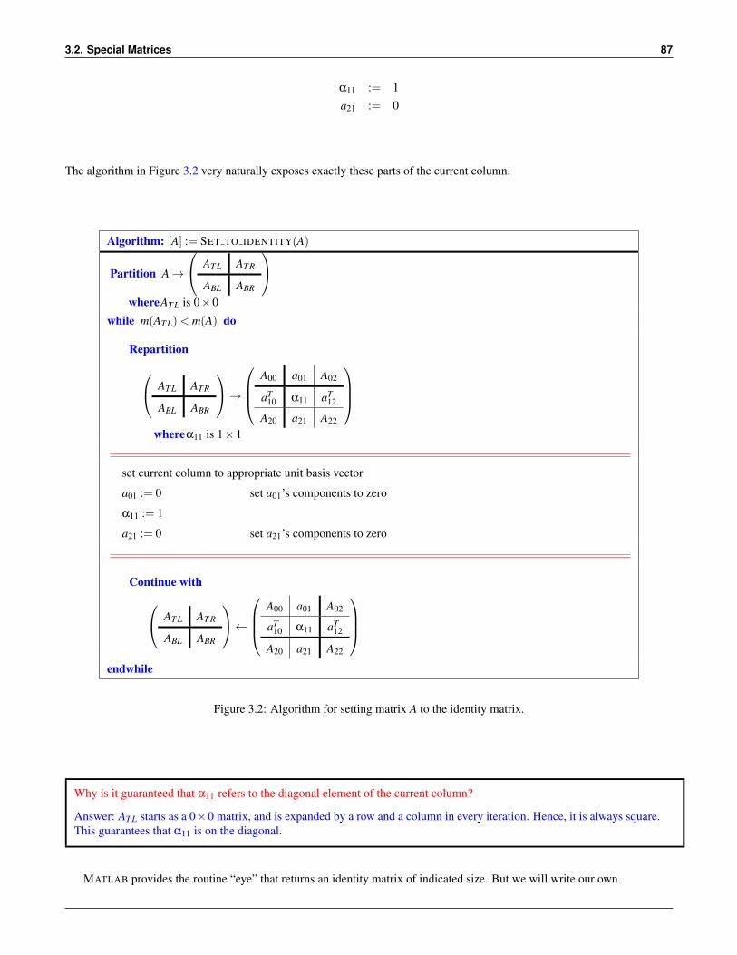
α11 := 1a21 := 0
The algorithm in Figure 3.2 very naturally exposes exactly these parts of the current column.
Algorithm: [A] := SET TO IDENTITY(A)
Partition A→
AT L AT R
ABL ABR
whereAT L is 0×0
while m(AT L)< m(A) do
Repartition AT L AT R
ABL ABR
→
A00 a01 A02
aT10 α11 aT
12
A20 a21 A22
whereα11 is 1×1
set current column to appropriate unit basis vector
a01 := 0 set a01’s components to zero
α11 := 1
a21 := 0 set a21’s components to zero
Continue with AT L AT R
ABL ABR
←
A00 a01 A02
aT10 α11 aT
12
A20 a21 A22
endwhile
Figure 3.2: Algorithm for setting matrix A to the identity matrix.
Why is it guaranteed that α11 refers to the diagonal element of the current column?
Answer: AT L starts as a 0×0 matrix, and is expanded by a row and a column in every iteration. Hence, it is always square.This guarantees that α11 is on the diagonal.
MATLAB provides the routine “eye” that returns an identity matrix of indicated size. But we will write our own.
Week 3. Matrix-Vector Operations 88
Homework 3.2.2.2 With the FLAME API for MATLAB (FLAME@lab) implement the algorithm in Figure 3.2.You will use the functions laff zerov( x ) and laff onev( x ), which return a zero vector and vector of allones of the same size and shape (column or row) as input vector x, respectively. Try it yourself! (Hint: in Spark,you will want to pick Direction TL->BR.) Feel free to look at the below video if you get stuck.Some links that will come in handy:
• * Spark(alternatively, open the file * LAFF-2.0xM/Spark/index.html)
• * PictureFLAME(alternatively, open the file * LAFF-2.0xM/PictureFLAME/PictureFLAME.html)
You will need these in many future exercises. Bookmark them!
* View at edX
Homework 3.2.2.3 In the MATLAB Command Window, type
A = eye( 4,4 )
What is the result?
Homework 3.2.2.4 Apply the identity matrix to Timmy Two Space. What happens?
1. Timmy shifts off the grid.
2. Timmy disappears into the origin.
3. Timmy becomes a line on the x-axis.
4. Timmy becomes a line on the y-axis.
5. Timmy doesn’t change at all.
Homework 3.2.2.5 The trace of a matrix equals the sum of the diagonal elements. What is the trace of the identityI ∈ Rn×n?
3.2.3 Diagonal Matrices
* View at edXLet LD : Rn→ Rn be the function defined for every x ∈ Rn as
L(
χ0
χ1...
χn−1
) =
δ0χ0
δ1χ1...
δn−1χn−1
),
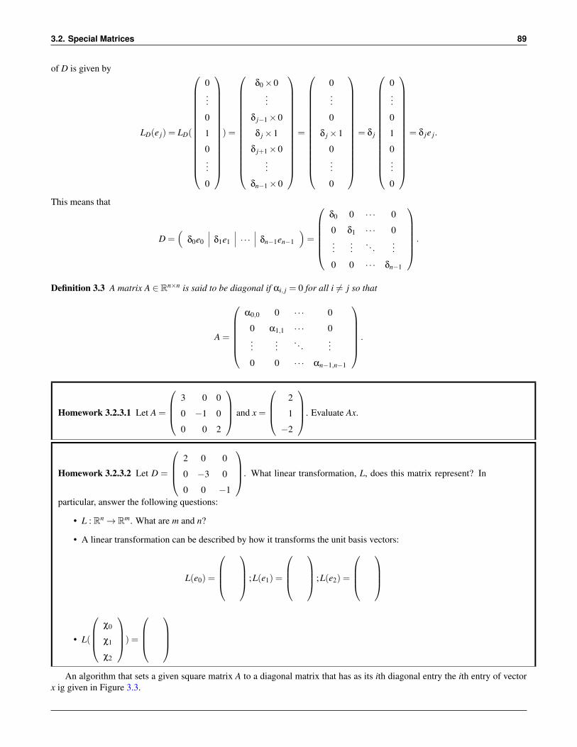
where δ0, . . . ,δn−1 are constants.Here, we will denote the matrix that represents LD by the letter D. Once again, by the definition of a matrix, the jth column
3.2. Special Matrices 89
of D is given by
LD(e j) = LD(
0...
0
1
0...
0
) =
δ0×0...
δ j−1×0
δ j×1
δ j+1×0...
δn−1×0
=
0...
0
δ j×1
0...
0
= δ j
0...
0
1
0...
0
= δ je j.
This means that
D =(
δ0e0 δ1e1 · · · δn−1en−1
)=
δ0 0 · · · 0
0 δ1 · · · 0...
.... . .
...
0 0 · · · δn−1
.
Definition 3.3 A matrix A ∈ Rn×n is said to be diagonal if αi, j = 0 for all i 6= j so that
A =
α0,0 0 · · · 0
0 α1,1 · · · 0...
.... . .
...
0 0 · · · αn−1,n−1
.
Homework 3.2.3.1 Let A =
3 0 0
0 −1 0
0 0 2
and x =
2
1
−2
. Evaluate Ax.
Homework 3.2.3.2 Let D =
2 0 0
0 −3 0
0 0 −1
. What linear transformation, L, does this matrix represent? In
particular, answer the following questions:
• L : Rn→ Rm. What are m and n?
• A linear transformation can be described by how it transforms the unit basis vectors:
L(e0) =
;L(e1) =
;L(e2) =
• L(
χ0
χ1
χ2
) =
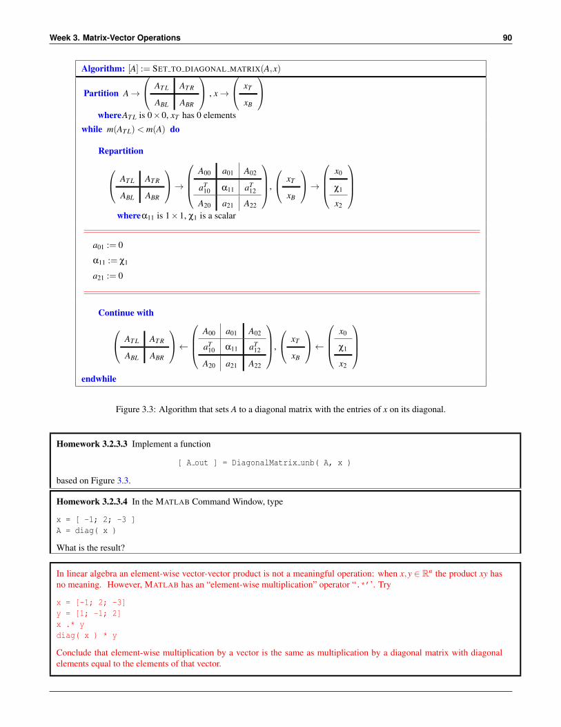
An algorithm that sets a given square matrix A to a diagonal matrix that has as its ith diagonal entry the ith entry of vectorx ig given in Figure 3.3.
Week 3. Matrix-Vector Operations 90
Algorithm: [A] := SET TO DIAGONAL MATRIX(A,x)
Partition A→
AT L AT R
ABL ABR
, x→
xT
xB
whereAT L is 0×0, xT has 0 elements
while m(AT L)< m(A) do
Repartition AT L AT R
ABL ABR
→
A00 a01 A02
aT10 α11 aT
12
A20 a21 A22
,
xT
xB
→
x0
χ1
x2
whereα11 is 1×1, χ1 is a scalar
a01 := 0
α11 := χ1
a21 := 0
Continue with AT L AT R
ABL ABR
←
A00 a01 A02
aT10 α11 aT
12
A20 a21 A22
,
xT
xB
←
x0
χ1
x2
endwhile
Figure 3.3: Algorithm that sets A to a diagonal matrix with the entries of x on its diagonal.
Homework 3.2.3.3 Implement a function
[ A out ] = DiagonalMatrix unb( A, x )
based on Figure 3.3.
Homework 3.2.3.4 In the MATLAB Command Window, type
x = [ -1; 2; -3 ]A = diag( x )
What is the result?
In linear algebra an element-wise vector-vector product is not a meaningful operation: when x,y ∈ Rn the product xy hasno meaning. However, MATLAB has an “element-wise multiplication” operator “.*’’. Try
x = [-1; 2; -3]y = [1; -1; 2]x .* ydiag( x ) * y
Conclude that element-wise multiplication by a vector is the same as multiplication by a diagonal matrix with diagonalelements equal to the elements of that vector.
3.2. Special Matrices 91
Homework 3.2.3.5 Apply the diagonal matrix
−1 0
0 2
to Timmy Two Space. What happens?
1. Timmy shifts off the grid.
2. Timmy is rotated.
3. Timmy doesn’t change at all.
4. Timmy is flipped with respect to the vertical axis.
5. Timmy is stretched by a factor two in the vertical direction.
Homework 3.2.3.6 Compute the trace of
−1 0
0 2
.
3.2.4 Triangular Matrices
* View at edX
Homework 3.2.4.1 Let LU : R3 → R3 be defined as LU (
χ0
χ1
χ2
) =
2χ0−χ1 +χ2
3χ1−χ2
−2χ2
. We have proven for
similar functions that they are linear transformations, so we will skip that part. What matrix, U , represents thislinear transformation?
A matrix like U in the above practice is called a triangular matrix. In particular, it is an upper triangular matrix.
Week 3. Matrix-Vector Operations 92
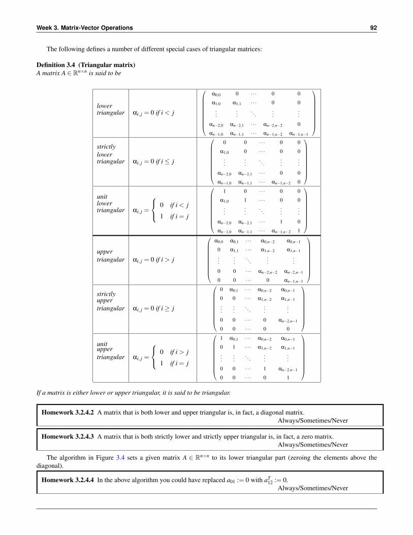
The following defines a number of different special cases of triangular matrices:
Definition 3.4 (Triangular matrix)A matrix A ∈ Rn×n is said to be
lowertriangular αi, j = 0 if i < j
α0,0 0 · · · 0 0
α1,0 α1,1 · · · 0 0...
.... . .
......
αn−2,0 αn−2,1 · · · αn−2,n−2 0
αn−1,0 αn−1,1 · · · αn−1,n−2 αn−1,n−1
strictlylowertriangular αi, j = 0 if i≤ j
0 0 · · · 0 0
α1,0 0 · · · 0 0...
.... . .
......
αn−2,0 αn−2,1 · · · 0 0
αn−1,0 αn−1,1 · · · αn−1,n−2 0
unitlowertriangular αi, j =
0 if i < j
1 if i = j
1 0 · · · 0 0
α1,0 1 · · · 0 0...
.... . .
......
αn−2,0 αn−2,1 · · · 1 0
αn−1,0 αn−1,1 · · · αn−1,n−2 1
uppertriangular αi, j = 0 if i > j
α0,0 α0,1 · · · α0,n−2 α0,n−1
0 α1,1 · · · α1,n−2 α1,n−1
......
. . ....
...
0 0 · · · αn−2,n−2 αn−2,n−1
0 0 · · · 0 αn−1,n−1
strictlyuppertriangular αi, j = 0 if i≥ j
0 α0,1 · · · α0,n−2 α0,n−1
0 0 · · · α1,n−2 α1,n−1
......
. . ....
...
0 0 · · · 0 αn−2,n−1
0 0 · · · 0 0
unituppertriangular αi, j =
0 if i > j
1 if i = j
1 α0,1 · · · α0,n−2 α0,n−1
0 1 · · · α1,n−2 α1,n−1
......
. . ....
...
0 0 · · · 1 αn−2,n−1
0 0 · · · 0 1
If a matrix is either lower or upper triangular, it is said to be triangular.
Homework 3.2.4.2 A matrix that is both lower and upper triangular is, in fact, a diagonal matrix.Always/Sometimes/Never
Homework 3.2.4.3 A matrix that is both strictly lower and strictly upper triangular is, in fact, a zero matrix.Always/Sometimes/Never
The algorithm in Figure 3.4 sets a given matrix A ∈ Rn×n to its lower triangular part (zeroing the elements above thediagonal).
Homework 3.2.4.4 In the above algorithm you could have replaced a01 := 0 with aT12 := 0.
Always/Sometimes/Never
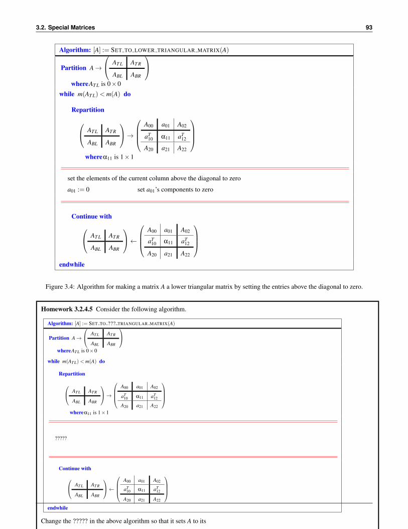
3.2. Special Matrices 93
Algorithm: [A] := SET TO LOWER TRIANGULAR MATRIX(A)
Partition A→
AT L AT R
ABL ABR
whereAT L is 0×0
while m(AT L)< m(A) do
Repartition AT L AT R
ABL ABR
→
A00 a01 A02
aT10 α11 aT
12
A20 a21 A22
whereα11 is 1×1
set the elements of the current column above the diagonal to zero
a01 := 0 set a01’s components to zero
Continue with AT L AT R
ABL ABR
←
A00 a01 A02
aT10 α11 aT
12
A20 a21 A22
endwhile
Figure 3.4: Algorithm for making a matrix A a lower triangular matrix by setting the entries above the diagonal to zero.
Homework 3.2.4.5 Consider the following algorithm.
Algorithm: [A] := SET TO ??? TRIANGULAR MATRIX(A)
Partition A→
AT L AT R
ABL ABR
whereAT L is 0×0
while m(AT L)< m(A) do
Repartition
AT L AT R
ABL ABR
→
A00 a01 A02
aT10 α11 aT
12
A20 a21 A22
whereα11 is 1×1
?????
Continue with
AT L AT R
ABL ABR
←
A00 a01 A02
aT10 α11 aT
12
A20 a21 A22
endwhile
Change the ????? in the above algorithm so that it sets A to its
• Upper triangular part. (Set to upper triangular matrix unb)
• Strictly upper triangular part. (Set to strictly upper triangular matrix unb)
• Unit upper triangular part. (Set to unit upper triangular matrix unb)
• Strictly lower triangular part. (Set to strictly lower triangular matrix unb)
• Unit lower triangular part. (Set to unit lower triangular matrix unb)
Week 3. Matrix-Vector Operations 94
The MATLAB functions tril and triu, when given an n× n matrix A, return the lower and upper triangular parts of A,respectively. The strictly lower and strictly upper triangular parts of A can be extracted by the calls tril( A, -1 ) and triu(A, 1 ), respectively. We now write our own routines that sets the appropriate entries in a matrix to zero.
Homework 3.2.4.6 Implement functions for each of the algorithms from the last homework. In other words,implement functions that, given a matrix A, return a matrix equal to
• the upper triangular part. (Set to upper triangular matrix)
• the strictly upper triangular part. (Set to strictly upper triangular matrix)
• the unit upper triangular part. (Set to unit upper triangular matrix)
• strictly lower triangular part. (Set to strictly lower triangular matrix)
• unit lower triangular part. (Set to unit lower triangular matrix)
(Implement as many as you enjoy implementing. Then move on.)
Homework 3.2.4.7 In MATLAB try this:
A = [ 1,2,3;4,5,6;7,8,9 ]tril( A )tril( A, -1 )tril( A, -1 ) + eye( size( A ) )triu( A )triu( A, 1 )triu( A, 1 ) + eye( size( A ) )
Homework 3.2.4.8 Apply
1 1
0 1
to Timmy Two Space. What happens to Timmy?
1. Timmy shifts off the grid.
2. Timmy becomes a line on the x-axis.
3. Timmy becomes a line on the y-axis.
4. Timmy is skewed to the right.
5. Timmy doesn’t change at all.
3.2.5 Transpose Matrix
* View at edX
Definition 3.5 Let A ∈Rm×n and B ∈Rn×m. Then B is said to be the transpose of A if, for 0≤ i < m and 0≤ j < n, β j,i = αi, j.The transpose of a matrix A is denoted by AT so that B = AT .
We have already used T to indicate a row vector, which is consistent with the above definition: it is a column vector thathas been transposed.
3.2. Special Matrices 95
Homework 3.2.5.1 Let A =
−1 0 2 1
2 −1 1 2
3 1 −1 3
and x =
−1
2
4
. What are AT and xT ?
Clearly, (AT )T = A.
Notice that the columns of matrix A become the rows of matrix AT . Similarly, the rows of matrix A become the columns ofmatrix AT .
The following algorithm sets a given matrix B ∈ Rn×m to the transpose of a given matrix A ∈ Rm×n:
Algorithm: [B] := TRANSPOSE(A,B)
Partition A→(
AL AR
), B→
BT
BB
whereAL has 0 columns, BT has 0 rows
while n(AL)< n(A) do
Repartition
(AL AR
)→(
A0 a1 A2
),
BT
BB
→
B0
bT1
B2
wherea1 has 1 column, b1 has 1 row
bT1 := aT
1 (Set the current row of B to the current col-umn of A)
Continue with
(AL AR
)←(
A0 a1 A2
),
BT
BB
←
B0
bT1
B2
endwhile
The T in bT1 is part of indicating that bT
1 is a row. The T in aT1 in the assignment changes the column vector a1 into a row
vector so that it can be assigned to bT1 .

Week 3. Matrix-Vector Operations 96
Homework 3.2.5.2 Consider the following algorithm.
Algorithm: [B] := TRANSPOSE ALTERNATIVE(A,B)
Partition A→
AT
AB
, B→(
BL BR
)whereAT has 0 rows, BL has 0 columns
while m(AT )< m(A) do
Repartition
AT
AB
→
A0
aT1
A2
,(
BL BR
)→(
B0 b1 B2
)wherea1 has 1 row, b1 has 1 column
Continue with
AT
AB
←
A0
aT1
A2
,(
BL BR
)←(
B0 b1 B2
)endwhile
Modify the above algorithm so that it copies rows of A into columns of B.
Homework 3.2.5.3 Implement functions
• Transpose unb( A, B )
• Transpose alternative unb( A, B )
Homework 3.2.5.4 The transpose of a lower triangular matrix is an upper triangular matrix.Always/Sometimes/Never
Homework 3.2.5.5 The transpose of a strictly upper triangular matrix is a strictly lower triangular matrix.Always/Sometimes/Never
Homework 3.2.5.6 The transpose of the identity is the identity.Always/Sometimes/Never
Homework 3.2.5.7 Evaluate
•
0 1
1 0
T
=
•
0 1
−1 0
T
=
3.2. Special Matrices 97
Homework 3.2.5.8 If A = AT then A = I (the identity).True/False
3.2.6 Symmetric Matrices
* View at edXA matrix A ∈ Rn×n is said to be symmetric if A = AT .
In other words, if A ∈ Rn×n is symmetric, then αi, j = α j,i for all 0≤ i, j < n. Another way of expressing this is that
A =
α0,0 α0,1 · · · α0,n−2 α0,n−1
α0,1 α1,1 · · · α1,n−2 α1,n−1...
.... . .
......
α0,n−2 α1,n−2 · · · αn−2,n−2 αn−2,n−1
α0,n−1 α1,n−1 · · · αn−2,n−1 αn−1,n−1
and
A =
α0,0 α1,0 · · · αn−2,0 αn−1,0
α1,0 α1,1 · · · αn−2,1 αn−1,1...
.... . .
......
αn−2,0 αn−2,1 · · · αn−2,n−2 αn−1,n−2
αn−1,0 αn−1,1 · · · αn−1,n−2 αn−1,n−1
.
Homework 3.2.6.1 Assume the below matrices are symmetric. Fill in the remaining elements.2 � −1
−2 1 −3
� � −1
;
2 � �
−2 1 �
−1 3 −1
;
2 1 −1
� 1 −3
� � −1
.
Homework 3.2.6.2 A triangular matrix that is also symmetric is, in fact, a diagonal matrix. Always/Some-times/Never
The nice thing about symmetric matrices is that only approximately half of the entries need to be stored. Often, only thelower triangular or only the upper triangular part of a symmetric matrix is stored. Indeed: Let A be symmetric, let L be thelower triangular matrix stored in the lower triangular part of A, and let L is the strictly lower triangular matrix stored in thestrictly lower triangular part of A. Then A = L+ LT :
A =
α0,0 α1,0 · · · αn−2,0 αn−1,0
α1,0 α1,1 · · · αn−2,1 αn−1,1
......
. . ....
...
αn−2,0 αn−2,1 · · · αn−2,n−2 αn−1,n−2
αn−1,0 αn−1,1 · · · αn−1,n−2 αn−1,n−1
=
α0,0 0 · · · 0 0
α1,0 α1,1 · · · 0 0...
.... . .
......
αn−2,0 αn−2,1 · · · αn−2,n−2 0
αn−1,0 αn−1,1 · · · αn−1,n−2 αn−1,n−1
+
0 α1,0 · · · αn−2,0 αn−1,0
0 0 · · · αn−2,1 αn−1,1
......
. . ....
...
0 0 · · · 0 αn−1,n−2
0 0 · · · 0 0
Week 3. Matrix-Vector Operations 98
=
α0,0 0 · · · 0 0
α1,0 α1,1 · · · 0 0...
.... . .
......
αn−2,0 αn−2,1 · · · αn−2,n−2 0
αn−1,0 αn−1,1 · · · αn−1,n−2 αn−1,n−1
+
0 0 · · · 0 0
α1,0 0 · · · 0 0...
.... . .
......
αn−2,0 αn−2,1 · · · 0 0
αn−1,0 αn−1,1 · · · αn−1,n−2 0
T
.
Let A be symmetric and assume that A = L+ LT as discussed above. Assume that only L is stored in A and that we wouldlike to also set the upper triangular parts of A to their correct values (in other words, set the strictly upper triangular part of A toL). The following algorithm performs this operation, which we will call “symmetrizing” A:
Algorithm: [A] := SYMMETRIZE FROM LOWER TRIANGLE(A)
Partition A→
AT L AT R
ABL ABR
whereAT L is 0×0
while m(AT L)< m(A) do
Repartition AT L AT R
ABL ABR
→
A00 a01 A02
aT10 α11 aT
12
A20 a21 A22
whereα11 is 1×1
(set a01’s components to their symmetric parts below the diagonal)
a01 := (aT10)
T
Continue with AT L AT R
ABL ABR
←
A00 a01 A02
aT10 α11 aT
12
A20 a21 A22
endwhile
Homework 3.2.6.3 In the above algorithm one can replace a01 := aT10 by aT
12 = a21.Always/Sometimes/Never
3.3. Operations with Matrices 99
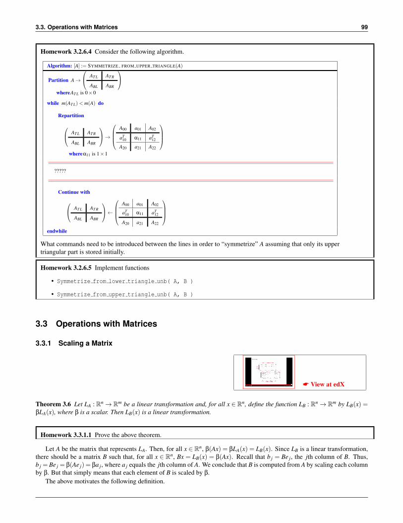
Homework 3.2.6.4 Consider the following algorithm.
Algorithm: [A] := SYMMETRIZE FROM UPPER TRIANGLE(A)
Partition A→
AT L AT R
ABL ABR
whereAT L is 0×0
while m(AT L)< m(A) do
Repartition
AT L AT R
ABL ABR
→
A00 a01 A02
aT10 α11 aT
12
A20 a21 A22
whereα11 is 1×1
?????
Continue with
AT L AT R
ABL ABR
←
A00 a01 A02
aT10 α11 aT
12
A20 a21 A22
endwhile
What commands need to be introduced between the lines in order to “symmetrize” A assuming that only its uppertriangular part is stored initially.
Homework 3.2.6.5 Implement functions
• Symmetrize from lower triangle unb( A, B )
• Symmetrize from upper triangle unb( A, B )
3.3 Operations with Matrices
3.3.1 Scaling a Matrix
* View at edX
Theorem 3.6 Let LA : Rn→ Rm be a linear transformation and, for all x ∈ Rn, define the function LB : Rn→ Rm by LB(x) =βLA(x), where β is a scalar. Then LB(x) is a linear transformation.
Homework 3.3.1.1 Prove the above theorem.
Let A be the matrix that represents LA. Then, for all x ∈ Rn, β(Ax) = βLA(x) = LB(x). Since LB is a linear transformation,there should be a matrix B such that, for all x ∈ Rn, Bx = LB(x) = β(Ax). Recall that b j = Be j, the jth column of B. Thus,b j = Be j = β(Ae j) = βa j, where a j equals the jth column of A. We conclude that B is computed from A by scaling each columnby β. But that simply means that each element of B is scaled by β.
The above motivates the following definition.
Week 3. Matrix-Vector Operations 100
If A ∈ Rm×n and β ∈ R, then
β
α0,0 α0,1 · · · α0,n−1
α1,0 α1,1 · · · α1,n−1...
......
αm−1,0 αm−1,1 · · · αm−1,n−1
=
βα0,0 βα0,1 · · · βα0,n−1
βα1,0 βα1,1 · · · βα1,n−1...
......
βαm−1,0 βαm−1,1 · · · βαm−1,n−1
.
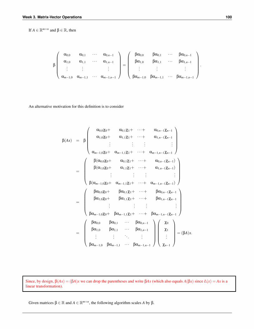
An alternative motivation for this definition is to consider
β(Ax) = β
α0,0χ0+ α0,1χ1+ · · ·+ α0,n−1χn−1
α1,0χ0+ α1,1χ1+ · · ·+ α1,n−1χn−1...
......
...
αm−1,0χ0+ αm−1,1χ1+ · · ·+ αm−1,n−1χn−1
=
β(α0,0χ0+ α0,1χ1+ · · ·+ α0,n−1χn−1)
β(α1,0χ0+ α1,1χ1+ · · ·+ α1,n−1χn−1)...
......
...
β(αm−1,0χ0+ αm−1,1χ1+ · · ·+ αm−1,n−1χn−1)
=
βα0,0χ0+ βα0,1χ1+ · · ·+ βα0,n−1χn−1
βα1,0χ0+ βα1,1χ1+ · · ·+ βα1,n−1χn−1...
......
...
βαm−1,0χ0+ βαm−1,1χ1+ · · ·+ βαm−1,n−1χn−1
=
βα0,0 βα0,1 · · · βα0,n−1
βα1,0 βα1,1 · · · βα1,n−1...
.... . .
...
βαm−1,0 βαm−1,1 · · · βαm−1,n−1
χ0
χ1...
χn−1
= (βA)x.
Since, by design, β(Ax) = (βA)x we can drop the parentheses and write βAx (which also equals A(βx) since L(x) = Ax is alinear transformation).
Given matrices β ∈ R and A ∈ Rm×n, the following algorithm scales A by β.
3.3. Operations with Matrices 101
Algorithm: [A] := SCALE MATRIX(β,A)
Partition A→(
AL AR
)whereAL has 0 columns
while n(AL)< n(A) do
Repartition(AL AR
)→(
A0 a1 A2
)wherea1 has 1 column
a1 := βa1 (Scale the current column of A)
Continue with(AL AR
)←(
A0 a1 A2
)endwhile
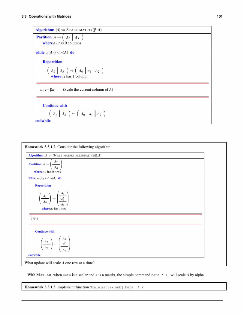
Homework 3.3.1.2 Consider the following algorithm.
Algorithm: [A] := SCALE MATRIX ALTERNATIVE(β,A)
Partition A→
AT
AB
whereAT has 0 rows
while m(AT )< m(A) do
Repartition
AT
AB
→
A0
aT1
A2
wherea1 has 1 row
?????
Continue with
AT
AB
←
A0
aT1
A2
endwhile
What update will scale A one row at a time?
With MATLAB, when beta is a scalar and A is a matrix, the simple command beta * A will scale A by alpha.
Homework 3.3.1.3 Implement function Scale matrix unb( beta, A ).
Week 3. Matrix-Vector Operations 102
Homework 3.3.1.4
* View at edXLet A ∈ Rn×n be a symmetric matrix and β ∈ R a scalar, βA is symmetric.
Always/Sometimes/Never
Homework 3.3.1.5
* View at edXLet A ∈ Rn×n be a lower triangular matrix and β ∈ R a scalar, βA is a lower triangular matrix.
Always/Sometimes/Never
Homework 3.3.1.6 Let A ∈ Rn×n be a diagonal matrix and β ∈ R a scalar, βA is a diagonal matrix.Always/Sometimes/Never
Homework 3.3.1.7 Let A ∈ Rm×n be a matrix and β ∈ R a scalar, (βA)T = βAT .Always/Sometimes/Never
3.3.2 Adding Matrices
* View at edX
Homework 3.3.2.1 The sum of two linear transformations is a linear transformation. More formally: Let LA :Rn→Rm and LB :Rn→Rm be two linear transformations. Let LC :Rn→Rm be defined by LC(x) = LA(x)+LB(x).LC is a linear transformation.
Always/Sometimes/Never
Now, let A, B, and C be the matrices that represent LA, LB, and LC in the above theorem, respectively. Then, for all x ∈ Rn,Cx = LC(x) = LA(x)+LB(x). What does c j, the jth column of C, equal?
c j =Ce j = LC(e j) = LA(e j)+LB(e j) = Ae j +Be j = a j +b j,
where a j, b j, and c j equal the jth columns of A, B, and C, respectively. Thus, the jth column of C equals the sum of thecorresponding columns of A and B. That simply means that each element of C equals the sum of the corresponding elements ofA and B.
If A,B ∈ Rm×n, then
A+B =
α0,0 α0,1 · · · α0,n−1
α1,0 α1,1 · · · α1,n−1...
......
αm−1,0 αm−1,1 · · · αm−1,n−1
+
β0,0 β0,1 · · · β0,n−1
β1,0 β1,1 · · · β1,n−1...
......
βm−1,0 βm−1,1 · · · βm−1,n−1
=
α0,0 +β0,0 α0,1 +β0,1 · · · α0,n−1 +β0,n−1
α1,0 +β1,0 α1,1 +β1,1 · · · α1,n−1 +β1,n−1...
......
αm−1,0 +βm−1,0 αm−1,1 +βm−1,1 · · · αm−1,n−1 +βm−1,n−1
.
Given matrices A,B ∈ Rm×n, the following algorithm adds B to A.
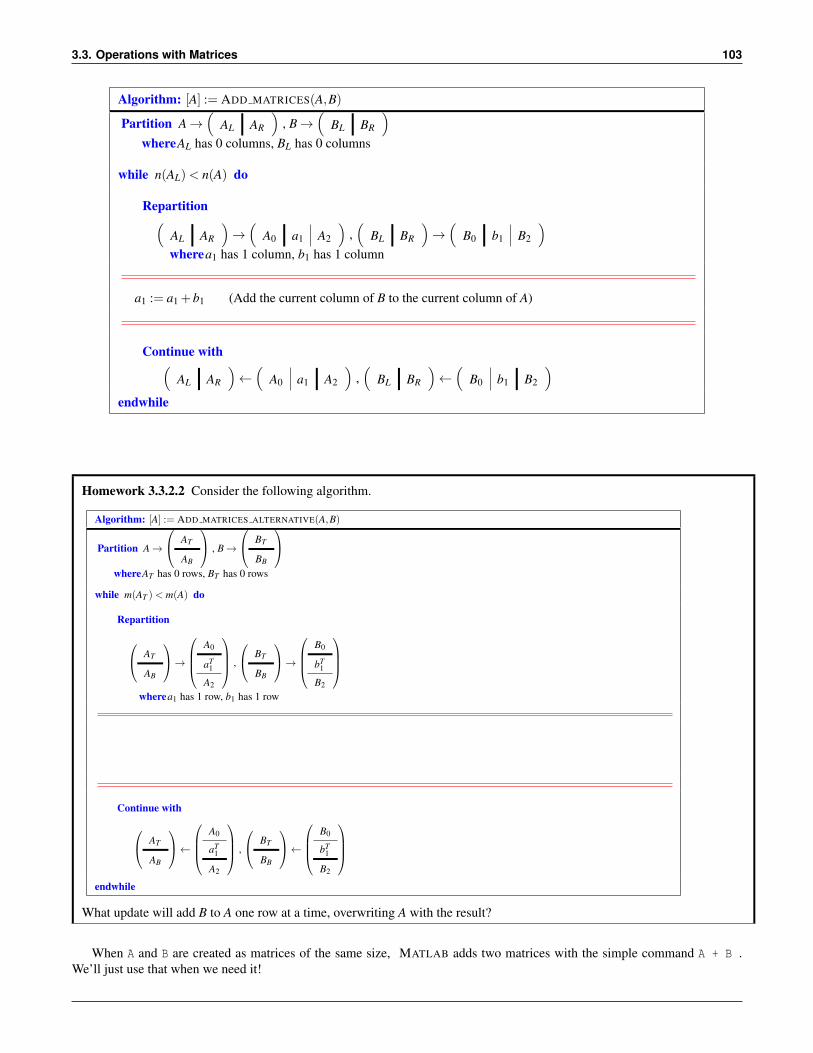
3.3. Operations with Matrices 103
Algorithm: [A] := ADD MATRICES(A,B)
Partition A→(
AL AR
), B→
(BL BR
)whereAL has 0 columns, BL has 0 columns
while n(AL)< n(A) do
Repartition(AL AR
)→(
A0 a1 A2
),(
BL BR
)→(
B0 b1 B2
)wherea1 has 1 column, b1 has 1 column
a1 := a1 +b1 (Add the current column of B to the current column of A)
Continue with(AL AR
)←(
A0 a1 A2
),(
BL BR
)←(
B0 b1 B2
)endwhile
Homework 3.3.2.2 Consider the following algorithm.
Algorithm: [A] := ADD MATRICES ALTERNATIVE(A,B)
Partition A→
AT
AB
, B→
BT
BB
whereAT has 0 rows, BT has 0 rows
while m(AT )< m(A) do
Repartition
AT
AB
→
A0
aT1
A2
,
BT
BB
→
B0
bT1
B2
wherea1 has 1 row, b1 has 1 row
Continue with
AT
AB
←
A0
aT1
A2
,
BT
BB
←
B0
bT1
B2
endwhile
What update will add B to A one row at a time, overwriting A with the result?
When A and B are created as matrices of the same size, MATLAB adds two matrices with the simple command A + B .We’ll just use that when we need it!
Week 3. Matrix-Vector Operations 104
Try this! In MATLAB execute
A = [ 1,2;3,4;5,6 ]B = [ -1,2;3,-4;5,6 ]C = A + B
Homework 3.3.2.3 Let A,B ∈ Rm×n. A+B = B+A.Always/Sometimes/Never
Homework 3.3.2.4 Let A,B,C ∈ Rm×n. (A+B)+C = A+(B+C).Always/Sometimes/Never
Homework 3.3.2.5 Let A,B ∈ Rm×n and γ ∈ R. γ(A+B) = γA+ γB.Always/Sometimes/Never
Homework 3.3.2.6 Let A ∈ Rm×n and β,γ ∈ R. (β+ γ)A = βA+ γA.Always/Sometimes/Never
Homework 3.3.2.7 Let A,B ∈ Rn×n. (A+B)T = AT +BT .Always/Sometimes/Never
Homework 3.3.2.8 Let A,B ∈ Rn×n be symmetric matrices. A+B is symmetric.Always/Sometimes/Never
Homework 3.3.2.9 Let A,B ∈ Rn×n be symmetric matrices. A−B is symmetric.Always/Sometimes/Never
Homework 3.3.2.10 Let A,B ∈ Rn×n be symmetric matrices and α,β ∈ R. αA+βB is symmetric.Always/Sometimes/Never
Homework 3.3.2.11 Let A,B ∈ Rn×n.
If A and B are lower triangular matrices then A+B is lower triangular.True/False
If A and B are strictly lower triangular matrices then A+B is strictly lower triangular.True/False
If A and B are unit lower triangular matrices then A+B is unit lower triangular.True/False
If A and B are upper triangular matrices then A+B is upper triangular.True/False
If A and B are strictly upper triangular matrices then A+B is strictly upper triangular.True/False
If A and B are unit upper triangular matrices then A+B is unit upper triangular.True/False
3.4. Matrix-Vector Multiplication Algorithms 105
Homework 3.3.2.12 Let A,B ∈ Rn×n.
If A and B are lower triangular matrices then A−B is lower triangular.True/False
If A and B are strictly lower triangular matrices then A−B is strictly lower triangular. True/False
If A and B are unit lower triangular matrices then A−B is strictly lower triangular. True/False
If A and B are upper triangular matrices then A−B is upper triangular. True/False
If A and B are strictly upper triangular matrices then A−B is strictly upper triangular. True/False
If A and B are unit upper triangular matrices then A−B is unit upper triangular. True/False
3.4 Matrix-Vector Multiplication Algorithms
3.4.1 Via Dot Products
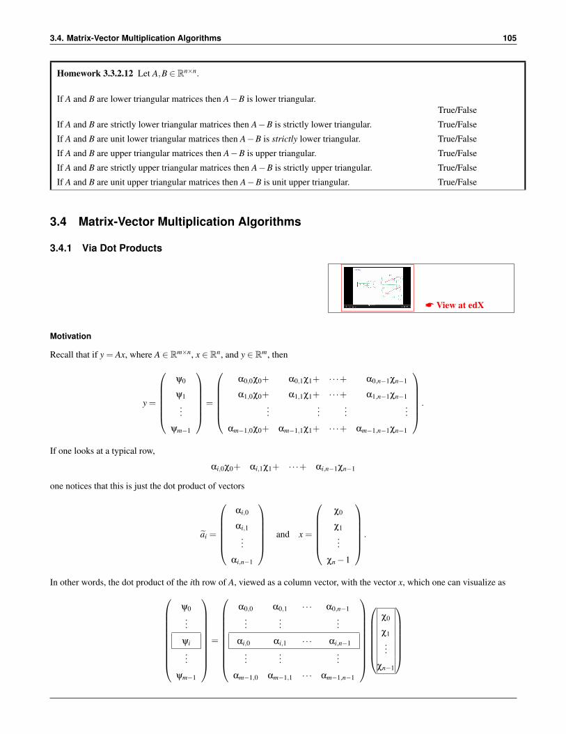
* View at edX
Motivation
Recall that if y = Ax, where A ∈ Rm×n, x ∈ Rn, and y ∈ Rm, then
y =
ψ0
ψ1...
ψm−1
=
α0,0χ0+ α0,1χ1+ · · ·+ α0,n−1χn−1
α1,0χ0+ α1,1χ1+ · · ·+ α1,n−1χn−1...
......
...
αm−1,0χ0+ αm−1,1χ1+ · · ·+ αm−1,n−1χn−1
.
If one looks at a typical row,
αi,0χ0+ αi,1χ1+ · · ·+ αi,n−1χn−1
one notices that this is just the dot product of vectors
ai =
αi,0
αi,1...
αi,n−1
and x =
χ0
χ1...
χn−1
.
In other words, the dot product of the ith row of A, viewed as a column vector, with the vector x, which one can visualize as
ψ0...
ψi...
ψm−1
=
α0,0 α0,1 · · · α0,n−1...
......
αi,0 αi,1 · · · αi,n−1...
......
αm−1,0 αm−1,1 · · · αm−1,n−1
χ0
χ1...
χn−1
Week 3. Matrix-Vector Operations 106
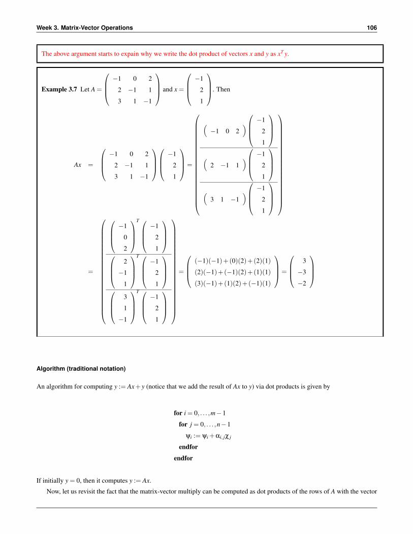
The above argument starts to expain why we write the dot product of vectors x and y as xT y.
Example 3.7 Let A =
−1 0 2
2 −1 1
3 1 −1
and x =
−1
2
1
. Then
Ax =
−1 0 2
2 −1 1
3 1 −1
−1
2
1
=
(−1 0 2
)−1
2
1
(
2 −1 1)
−1
2
1
(
3 1 −1)
−1
2
1
=
−1
0
2
T
−1
2
1
2
−1
1
T
−1
2
1
3
1
−1
T
−1
2
1
=
(−1)(−1)+(0)(2)+(2)(1)
(2)(−1)+(−1)(2)+(1)(1)
(3)(−1)+(1)(2)+(−1)(1)
=
3
−3
−2
Algorithm (traditional notation)
An algorithm for computing y := Ax+ y (notice that we add the result of Ax to y) via dot products is given by
for i = 0, . . . ,m−1
for j = 0, . . . ,n−1
ψi := ψi +αi, jχ j
endfor
endfor
If initially y = 0, then it computes y := Ax.
Now, let us revisit the fact that the matrix-vector multiply can be computed as dot products of the rows of A with the vector
3.4. Matrix-Vector Multiplication Algorithms 107
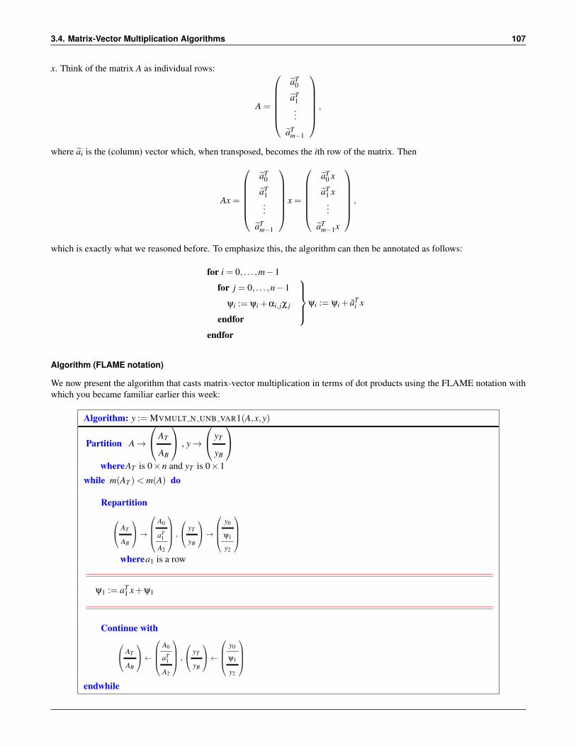
x. Think of the matrix A as individual rows:
A =
aT
0
aT1...
aTm−1
,
where ai is the (column) vector which, when transposed, becomes the ith row of the matrix. Then
Ax =
aT
0
aT1...
aTm−1
x =
aT
0 x
aT1 x...
aTm−1x
,
which is exactly what we reasoned before. To emphasize this, the algorithm can then be annotated as follows:
for i = 0, . . . ,m−1
for j = 0, . . . ,n−1
ψi := ψi +αi, jχ j
endfor
ψi := ψi + aTi x
endfor
Algorithm (FLAME notation)
We now present the algorithm that casts matrix-vector multiplication in terms of dot products using the FLAME notation withwhich you became familiar earlier this week:
Algorithm: y := MVMULT N UNB VAR1(A,x,y)
Partition A→
AT
AB
, y→
yT
yB
whereAT is 0×n and yT is 0×1
while m(AT )< m(A) do
Repartition
AT
AB
→
A0
aT1
A2
,
yT
yB
→
y0
ψ1
y2
wherea1 is a row
ψ1 := aT1 x+ψ1
Continue with AT
AB
←
A0
aT1
A2
,
yT
yB
←
y0
ψ1
y2
endwhile
Week 3. Matrix-Vector Operations 108
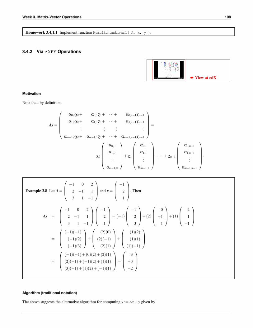
Homework 3.4.1.1 Implement function Mvmult n unb var1( A, x, y ).
3.4.2 Via AXPY Operations
* View at edX
Motivation
Note that, by definition,
Ax =
α0,0χ0+ α0,1χ1+ · · ·+ α0,n−1χn−1
α1,0χ0+ α1,1χ1+ · · ·+ α1,n−1χn−1...
......
...
αm−1,0χ0+ αm−1,1χ1+ · · ·+ αm−1,n−1χn−1
=
χ0
α0,0
α1,0...
αm−1,0
+χ1
α0,1
α1,1...
αm−1,1
+ · · ·+χn−1
α0,n−1
α1,n−1...
αm−1,n−1
.
Example 3.8 Let A =
−1 0 2
2 −1 1
3 1 −1
and x =
−1
2
1
. Then
Ax =
−1 0 2
2 −1 1
3 1 −1
−1
2
1
= (−1)
−1
2
3
+(2)
0
−1
1
+(1)
2
1
−1
=
(−1)(−1)
(−1)(2)
(−1)(3)
+
(2)(0)
(2)(−1)
(2)(1)
+
(1)(2)
(1)(1)
(1)(−1)
=
(−1)(−1)+(0)(2)+(2)(1)
(2)(−1)+(−1)(2)+(1)(1)
(3)(−1)+(1)(2)+(−1)(1)
=
3
−3
−2
Algorithm (traditional notation)
The above suggests the alternative algorithm for computing y := Ax+ y given by
3.4. Matrix-Vector Multiplication Algorithms 109
for j = 0, . . . ,n−1
for i = 0, . . . ,m−1
ψi := ψi +αi, jχ j
endfor
endfor
If we let a j denote the vector that equals the jth column of A, then
A =(
a0 a1 · · · an−1
)
and
Ax = χ0
α0,0
α1,0...
αm−1,0
︸ ︷︷ ︸
a0
+χ1
α0,1
α1,1...
αm−1,1
︸ ︷︷ ︸
a1
+ · · ·+χn−1
α0,n−1
α1,n−1...
αm−1,n−1
︸ ︷︷ ︸
an−1
= χ0a0 +χ1a1 + · · ·+χn−1an−1.
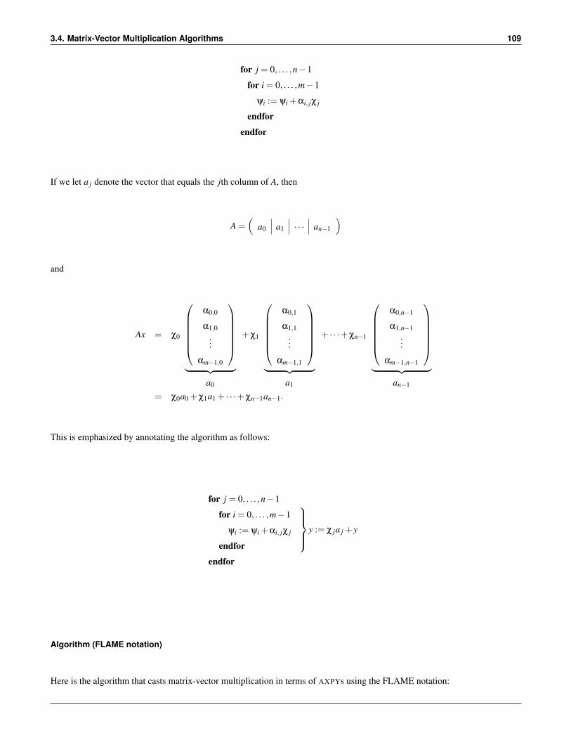
This is emphasized by annotating the algorithm as follows:
for j = 0, . . . ,n−1
for i = 0, . . . ,m−1
ψi := ψi +αi, jχ j
endfor
y := χ ja j + y
endfor
Algorithm (FLAME notation)
Here is the algorithm that casts matrix-vector multiplication in terms of AXPYs using the FLAME notation:
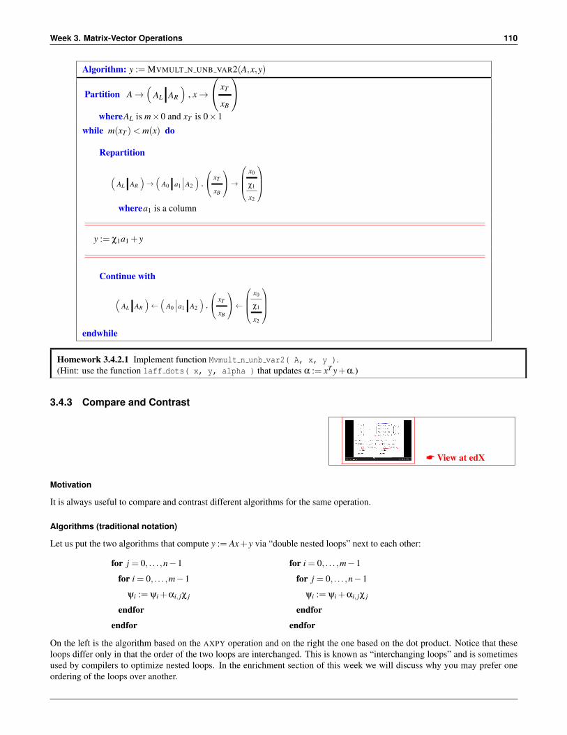
Week 3. Matrix-Vector Operations 110
Algorithm: y := MVMULT N UNB VAR2(A,x,y)
Partition A→(
AL AR
), x→
xT
xB
whereAL is m×0 and xT is 0×1
while m(xT )< m(x) do
Repartition
(AL AR
)→(
A0 a1 A2
),
xT
xB
→
x0
χ1
x2
wherea1 is a column
y := χ1a1 + y
Continue with
(AL AR
)←(
A0 a1 A2
),
xT
xB
←
x0
χ1
x2
endwhile
Homework 3.4.2.1 Implement function Mvmult n unb var2( A, x, y ).(Hint: use the function laff dots( x, y, alpha ) that updates α := xT y+α.)
3.4.3 Compare and Contrast
* View at edX
Motivation
It is always useful to compare and contrast different algorithms for the same operation.
Algorithms (traditional notation)
Let us put the two algorithms that compute y := Ax+ y via “double nested loops” next to each other:
for j = 0, . . . ,n−1
for i = 0, . . . ,m−1
ψi := ψi +αi, jχ j
endfor
endfor
for i = 0, . . . ,m−1
for j = 0, . . . ,n−1
ψi := ψi +αi, jχ j
endfor
endfor
On the left is the algorithm based on the AXPY operation and on the right the one based on the dot product. Notice that theseloops differ only in that the order of the two loops are interchanged. This is known as “interchanging loops” and is sometimesused by compilers to optimize nested loops. In the enrichment section of this week we will discuss why you may prefer oneordering of the loops over another.
3.4. Matrix-Vector Multiplication Algorithms 111
The above explains, in part, why we chose to look at y := Ax+ y rather than y := Ax. For y := Ax+ y, the two algorithmsdiffer only in the order in which the loops appear. To compute y := Ax, one would have to initialize each component ofy to zero, ψi := 0. Depending on where in the algorithm that happens, transforming an algorithm that computes y := Axelements of y at a time (the inner loop implements a dot product) into an algorithm that computes with columns of A (theinner loop implements an AXPY operation) gets trickier.
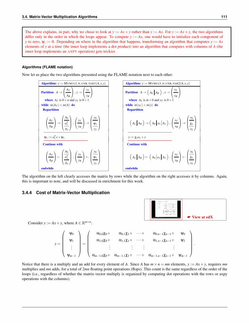
Algorithms (FLAME notation)
Now let us place the two algorithms presented using the FLAME notation next to each other:
Algorithm: y := MVMULT N UNB VAR1(A,x,y)
Partition A→
AT
AB
, y→
yT
yB
where AT is 0×n and yT is 0×1
while m(AT )< m(A) doRepartition
AT
AB
→
A0
aT1
A2
,
yT
yB
→
y0
ψ1
y2
ψ1 := aT
1 x+ψ1
Continue with
AT
AB
←
A0
aT1
A2
,
yT
yB
←
y0
ψ1
y2
endwhile
Algorithm: y := MVMULT N UNB VAR2(A,x,y)
Partition A→(
AL AR
), x→
xT
xB
where AL is m×0 and xT is 0×1
while m(xT )< m(x) doRepartition
(AL AR
)→(
A0 a1 A2
),
xT
xB
→
x0
χ1
x2
y := χ1a1 + y
Continue with
(AL AR
)←(
A0 a1 A2
),
xT
xB
←
x0
χ1
x2
endwhile
The algorithm on the left clearly accesses the matrix by rows while the algorithm on the right accesses it by columns. Again,this is important to note, and will be discussed in enrichment for this week.
3.4.4 Cost of Matrix-Vector Multiplication
* View at edXConsider y := Ax+ y, where A ∈ Rm×n:
y =
ψ0
ψ1...
ψm−1
=
α0,0χ0+ α0,1χ1+ · · ·+ α0,n−1χn−1+ ψ0
α1,0χ0+ α1,1χ1+ · · ·+ α1,n−1χn−1+ ψ2...
......
...
αm−1,0χ0+ αm−1,1χ1+ · · ·+ αm−1,n−1χn−1+ ψm−1
.
Notice that there is a multiply and an add for every element of A. Since A has m×n = mn elements, y := Ax+ y, requires mnmultiplies and mn adds, for a total of 2mn floating point operations (flops). This count is the same regardless of the order of theloops (i.e., regardless of whether the matrix-vector multiply is organized by computing dot operations with the rows or axpyoperations with the columns).
Week 3. Matrix-Vector Operations 112
3.5 Wrap Up
3.5.1 Homework
No additional homework this week. You have done enough...
3.5.2 Summary
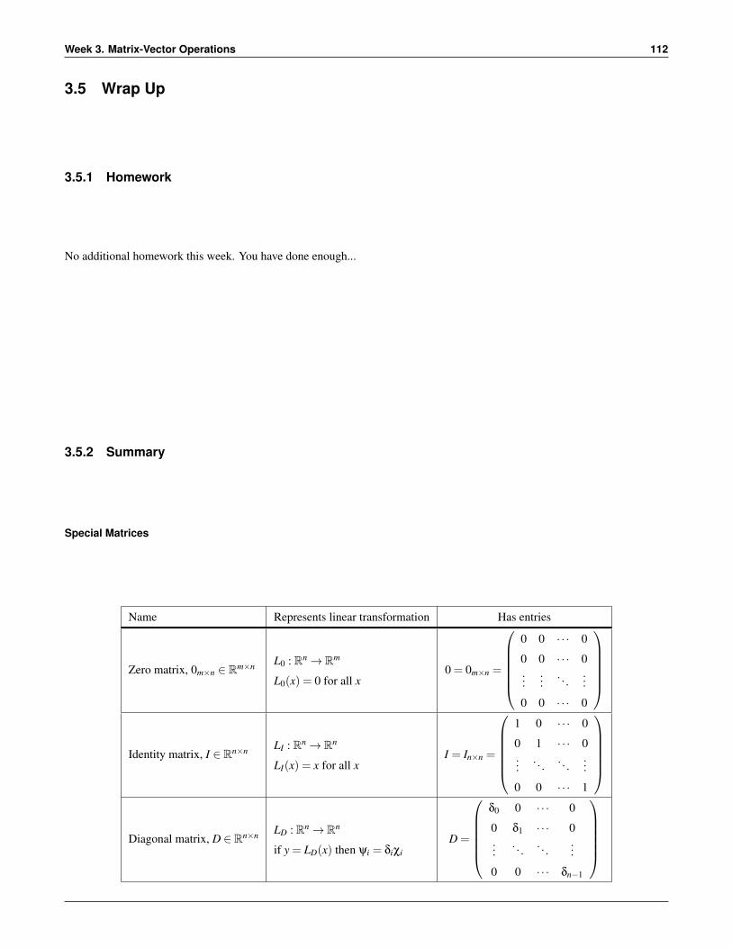
Special Matrices
Name Represents linear transformation Has entries
Zero matrix, 0m×n ∈ Rm×n L0 : Rn→ Rm
L0(x) = 0 for all x0 = 0m×n =
0 0 · · · 0
0 0 · · · 0...
.... . .
...
0 0 · · · 0
Identity matrix, I ∈ Rn×n LI : Rn→ Rn
LI(x) = x for all xI = In×n =
1 0 · · · 0
0 1 · · · 0...
. . . . . ....
0 0 · · · 1
Diagonal matrix, D ∈ Rn×n LD : Rn→ Rn
if y = LD(x) then ψi = δiχiD =
δ0 0 · · · 0
0 δ1 · · · 0...
. . . . . ....
0 0 · · · δn−1
3.5. Wrap Up 113
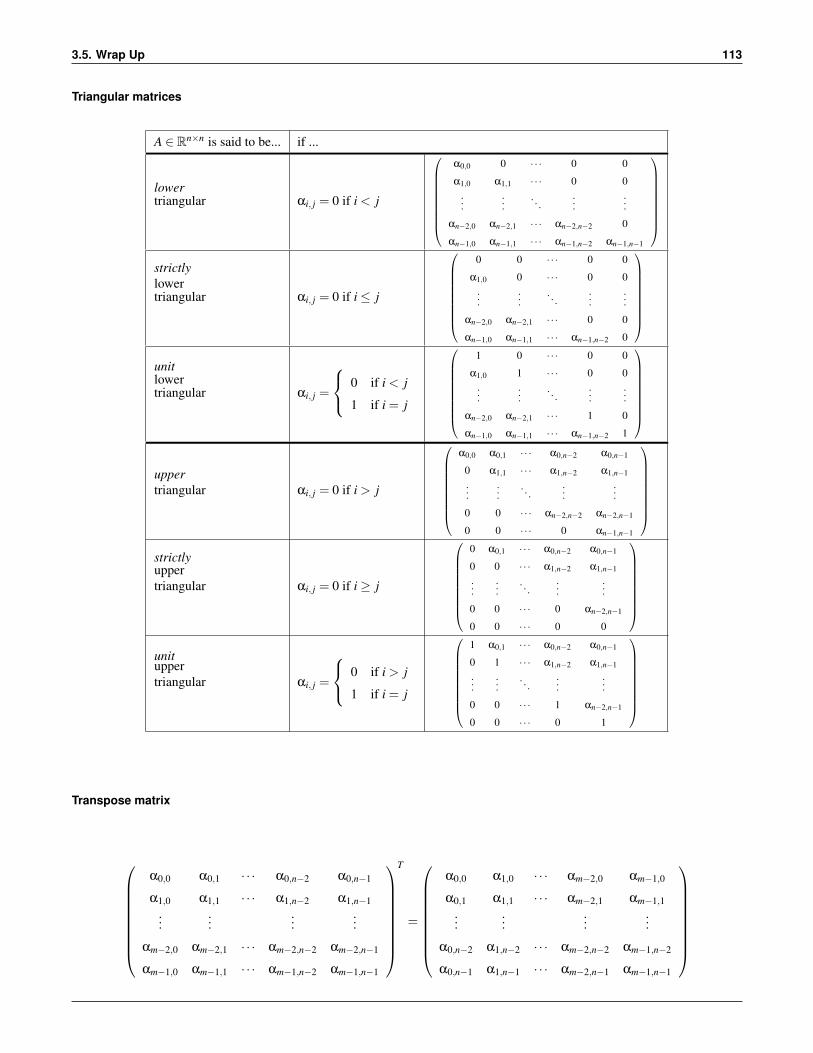
Triangular matrices
A ∈ Rn×n is said to be... if ...
lowertriangular αi, j = 0 if i < j
α0,0 0 · · · 0 0
α1,0 α1,1 · · · 0 0...
.... . .
......
αn−2,0 αn−2,1 · · · αn−2,n−2 0
αn−1,0 αn−1,1 · · · αn−1,n−2 αn−1,n−1
strictlylowertriangular αi, j = 0 if i≤ j
0 0 · · · 0 0
α1,0 0 · · · 0 0...
.... . .
......
αn−2,0 αn−2,1 · · · 0 0
αn−1,0 αn−1,1 · · · αn−1,n−2 0
unitlowertriangular αi, j =
0 if i < j
1 if i = j
1 0 · · · 0 0
α1,0 1 · · · 0 0...
.... . .
......
αn−2,0 αn−2,1 · · · 1 0
αn−1,0 αn−1,1 · · · αn−1,n−2 1
uppertriangular αi, j = 0 if i > j
α0,0 α0,1 · · · α0,n−2 α0,n−1
0 α1,1 · · · α1,n−2 α1,n−1
......
. . ....
...
0 0 · · · αn−2,n−2 αn−2,n−1
0 0 · · · 0 αn−1,n−1
strictlyuppertriangular αi, j = 0 if i≥ j
0 α0,1 · · · α0,n−2 α0,n−1
0 0 · · · α1,n−2 α1,n−1
......
. . ....
...
0 0 · · · 0 αn−2,n−1
0 0 · · · 0 0
unituppertriangular αi, j =
0 if i > j
1 if i = j
1 α0,1 · · · α0,n−2 α0,n−1
0 1 · · · α1,n−2 α1,n−1
......
. . ....
...
0 0 · · · 1 αn−2,n−1
0 0 · · · 0 1
Transpose matrix
α0,0 α0,1 · · · α0,n−2 α0,n−1
α1,0 α1,1 · · · α1,n−2 α1,n−1...
......
...
αm−2,0 αm−2,1 · · · αm−2,n−2 αm−2,n−1
αm−1,0 αm−1,1 · · · αm−1,n−2 αm−1,n−1
T
=
α0,0 α1,0 · · · αm−2,0 αm−1,0
α0,1 α1,1 · · · αm−2,1 αm−1,1...
......
...
α0,n−2 α1,n−2 · · · αm−2,n−2 αm−1,n−2
α0,n−1 α1,n−1 · · · αm−2,n−1 αm−1,n−1
Week 3. Matrix-Vector Operations 114
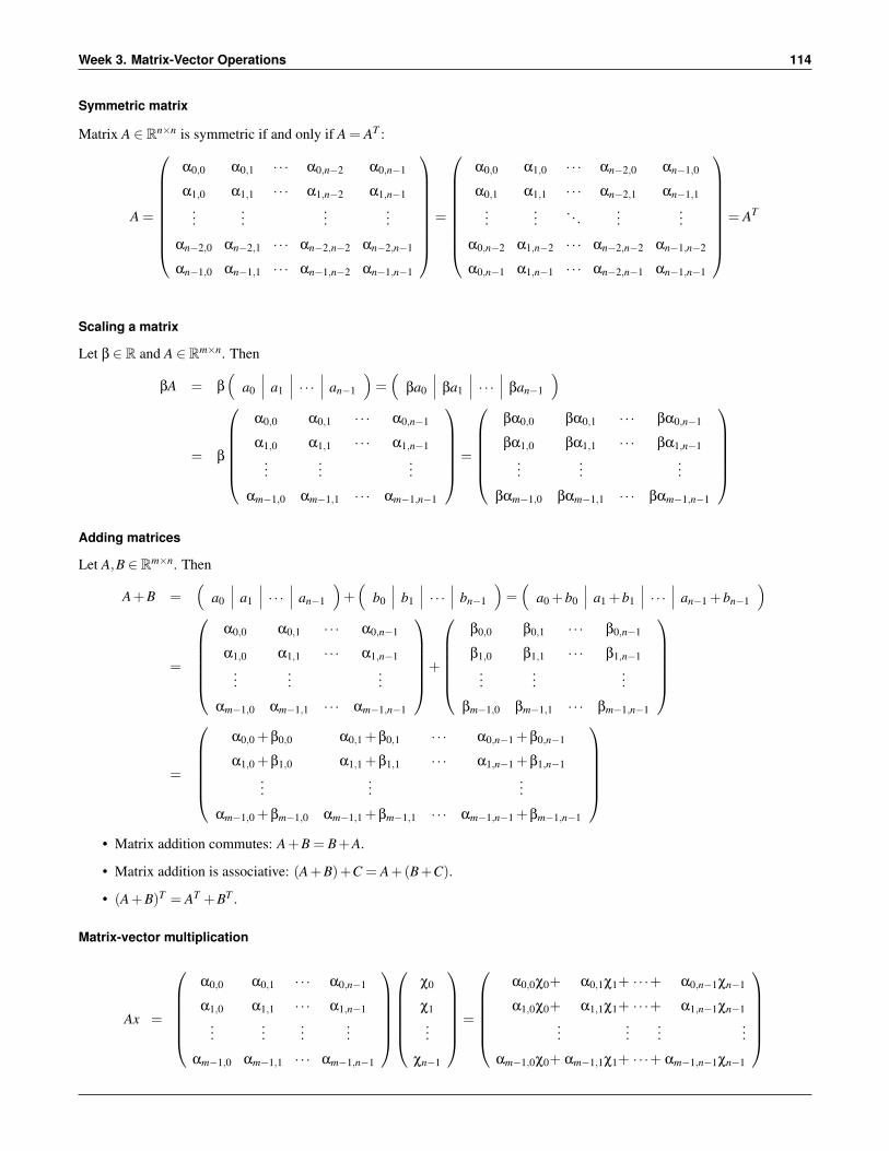
Symmetric matrix
Matrix A ∈ Rn×n is symmetric if and only if A = AT :
A =
α0,0 α0,1 · · · α0,n−2 α0,n−1
α1,0 α1,1 · · · α1,n−2 α1,n−1...
......
...
αn−2,0 αn−2,1 · · · αn−2,n−2 αn−2,n−1
αn−1,0 αn−1,1 · · · αn−1,n−2 αn−1,n−1
=
α0,0 α1,0 · · · αn−2,0 αn−1,0
α0,1 α1,1 · · · αn−2,1 αn−1,1...
.... . .
......
α0,n−2 α1,n−2 · · · αn−2,n−2 αn−1,n−2
α0,n−1 α1,n−1 · · · αn−2,n−1 αn−1,n−1
= AT
Scaling a matrix
Let β ∈ R and A ∈ Rm×n. Then
βA = β
(a0 a1 · · · an−1
)=(
βa0 βa1 · · · βan−1
)
= β
α0,0 α0,1 · · · α0,n−1
α1,0 α1,1 · · · α1,n−1...
......
αm−1,0 αm−1,1 · · · αm−1,n−1
=
βα0,0 βα0,1 · · · βα0,n−1
βα1,0 βα1,1 · · · βα1,n−1...
......
βαm−1,0 βαm−1,1 · · · βαm−1,n−1
Adding matrices
Let A,B ∈ Rm×n. Then
A+B =(
a0 a1 · · · an−1
)+(
b0 b1 · · · bn−1
)=(
a0 +b0 a1 +b1 · · · an−1 +bn−1
)
=
α0,0 α0,1 · · · α0,n−1
α1,0 α1,1 · · · α1,n−1...
......
αm−1,0 αm−1,1 · · · αm−1,n−1
+
β0,0 β0,1 · · · β0,n−1
β1,0 β1,1 · · · β1,n−1...
......
βm−1,0 βm−1,1 · · · βm−1,n−1
=
α0,0 +β0,0 α0,1 +β0,1 · · · α0,n−1 +β0,n−1
α1,0 +β1,0 α1,1 +β1,1 · · · α1,n−1 +β1,n−1...
......
αm−1,0 +βm−1,0 αm−1,1 +βm−1,1 · · · αm−1,n−1 +βm−1,n−1
• Matrix addition commutes: A+B = B+A.
• Matrix addition is associative: (A+B)+C = A+(B+C).
• (A+B)T = AT +BT .
Matrix-vector multiplication
Ax =
α0,0 α0,1 · · · α0,n−1
α1,0 α1,1 · · · α1,n−1...
......
...
αm−1,0 αm−1,1 · · · αm−1,n−1
χ0
χ1...
χn−1
=
α0,0χ0+ α0,1χ1+ · · ·+ α0,n−1χn−1
α1,0χ0+ α1,1χ1+ · · ·+ α1,n−1χn−1...
......
...
αm−1,0χ0+ αm−1,1χ1+ · · ·+ αm−1,n−1χn−1

3.5. Wrap Up 115
=(
a0 a1 · · · an−1
)
χ0
χ1...
χn−1
= χ0a0 +χ1a1 + · · ·+χn−1an−1
=
aT
0
aT1...
aTm−1
x =
aT
0 x
aT1 x...
aTm−1x

Week 3. Matrix-Vector Operations 116