Parallel Sparse Matrix-Vector and Matrix-Transpose-VectorMultiplication Using Compressed Sparse Blocks

Aydın Buluç∗aydin@cs.ucsb.edu

Jeremy T. Fineman†

jfineman@csail.mit.eduMatteo Frigo‡

matteo@cilk.com

John R. Gilbert∗gilbert@cs.ucsb.edu

Charles E. Leiserson†‡

cel@mit.edu

∗Dept. of Computer ScienceUniversity of California

Santa Barbara, CA 93106

†MIT CSAIL32 Vassar Street

Cambridge, MA 02139

‡Cilk Arts, Inc.55 Cambridge Street, Suite 200

Burlington, MA 01803

ABSTRACT

This paper introduces a storage format for sparse matrices, calledcompressed sparse blocks (CSB), which allows both Ax and ATx

to be computed efficiently in parallel, where A is an n× n sparsematrix with nnz ≥ n nonzeros and x is a dense n-vector. Our algo-rithms use Θ(nnz) work (serial running time) and Θ(

√n lgn) span

(critical-path length), yielding a parallelism of Θ(nnz/√

n lgn),which is amply high for virtually any large matrix. The storagerequirement for CSB is essentially the same as that for the more-standard compressed-sparse-rows (CSR) format, for which com-puting Ax in parallel is easy but ATx is difficult. Benchmark resultsindicate that on one processor, the CSB algorithms for Ax and ATx

run just as fast as the CSR algorithm for Ax, but the CSB algo-rithms also scale up linearly with processors until limited by off-chip memory bandwidth.

Categories and Subject Descriptors

F.2.1 [Analysis of Algorithms and Problem Complexity]: Nu-merical Algorithms and Problems—computations on matrices; G.4[Mathematics of Computing]: Mathematical Software—parallel

and vector implementations.

General Terms

Algorithms, Design, Experimentation, Performance, Theory.

Keywords

Compressed sparse blocks, compressed sparse columns, com-pressed sparse rows, matrix transpose, matrix-vector multiplica-tion, multithreaded algorithm, parallelism, span, sparse matrix,storage format, work.

This work was supported in part by the National Science Foundation underGrants 0540248, 0615215, 0712243, 0822896, and 0709385, and by MITLincoln Laboratory under contract 7000012980.

Permission to make digital or hard copies of all or part of this work forpersonal or classroom use is granted without fee provided that copies arenot made or distributed for profit or commercial advantage and that copiesbear this notice and the full citation on the first page. To copy otherwise, torepublish, to post on servers or to redistribute to lists, requires prior specificpermission and/or a fee.SPAA’09, August 11–13, 2009, Calgary, Alberta, Canada.Copyright 2009 ACM 978-1-60558-606-9/09/08 ...$10.00.

1. INTRODUCTIONWhen multiplying a large n× n sparse matrix A having nnz

nonzeros by a dense n-vector x, the memory bandwidth for readingA can limit overall performance. Consequently, most algorithms tocompute Ax store A in a compressed format. One simple “tuple”representation stores each nonzero of A as a triple consisting of itsrow index, its column index, and the nonzero value itself. Thisrepresentation, however, requires storing 2nnz row and column in-dices, in addition to the nonzeros. The current standard storage for-mat for sparse matrices in scientific computing, compressed sparse

rows (CSR) [32], is more efficient, because it stores only n+nnz in-dices or pointers. This reduction in storage of CSR compared withthe tuple representation tends to result in faster serial algorithms.

In the domain of parallel algorithms, however, CSR has its lim-itations. Although CSR lends itself to a simple parallel algorithmfor computing the matrix-vector product Ax, this storage formatdoes not admit an efficient parallel algorithm for computing theproduct ATx, where AT denotes the transpose of the matrix A —or equivalently, for computing the product xTA of a row vector xT

by A. Although one could use compressed sparse columns (CSC)

to compute ATx, many applications, including iterative linear sys-tem solvers such as biconjugate gradients and quasi-minimal resid-ual [32], require both Ax and ATx. One could transpose A explicitly,but computing the transpose for either CSR or CSC formats is ex-pensive. Moreover, since matrix-vector multiplication for sparsematrices is generally limited by memory bandwidth, it is desirableto find a storage format for which both Ax and ATx can be computedin parallel without performing more than nnz fetches of nonzerosfrom the memory to compute either product.

This paper presents a new storage format called compressed

sparse blocks (CSB) for representing sparse matrices. Like CSRand CSC, the CSB format requires only n + nnz words of storagefor indices. Because CSB does not favor rows over columns or viceversa, it admits efficient parallel algorithms for computing either Ax

or ATx, as well as for computing Ax when A is symmetric and onlyhalf the matrix is actually stored.

Previous work on parallel sparse matrix-vector multiplicationhas focused on reducing communication volume in a distributed-memory setting, often by using graph or hypergraph partitioningtechniques to find good data distributions for particular matrices( [7,38], for example). Good partitions generally exist for matriceswhose structures arise from numerical discretizations of partial dif-ferential equations in two or three spatial dimensions. Our work, bycontrast, is motivated by multicore and manycore architectures, inwhich parallelism and memory bandwidth are key resources. Our

0

100

200

300

400

500

1 2 3 4 5 6 7 8

MF

lops

/sec

Processors

CSB_SpMVCSB_SpMV_T

CSR_SpMV(Serial)CSR_SpMV_T(Serial)

Star-P(y=Ax)Star-P(y’=x’A)

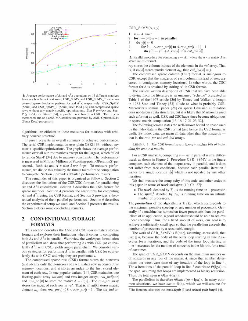
1: Average performance of Ax and ATx operations on 13 different matricesfrom our benchmark test suite. CSB_SpMV and CSB_SpMV_T use com-

pressed sparse blocks to perform Ax and ATx, respectively. CSR_SpMV(Serial) and CSR_SpMV_T (Serial) use OSKI [39] and compressed sparserows without any matrix-specific optimizations. Star-P (y=Ax) and Star-P (y’=x’A) use Star-P [34], a parallel code based on CSR. The experi-ments were run on a ccNUMA architecture powered by AMD Opteron 8214(Santa Rosa) processors.

algorithms are efficient in these measures for matrices with arbi-trary nonzero structure.

Figure 1 presents an overall summary of achieved performance.The serial CSR implementation uses plain OSKI [39] without anymatrix-specific optimizations. The graph shows the average perfor-mance over all our test matrices except for the largest, which failedto run on Star-P [34] due to memory constraints. The performanceis measured in Mflops (Millions of FLoating-point OPerationS) persecond. Both Ax and ATx take 2 nnz flops. To measure perfor-mance, we divide this value by the time it takes for the computationto complete. Section 7 provides detailed performance results.

The remainder of this paper is organized as follows. Section 2discusses the limitations of the CSR/CSC formats for parallelizingAx and ATx calculations. Section 3 describes the CSB format forsparse matrices. Section 4 presents the algorithms for computingAx and ATx using the CSB format, and Section 5 provides a theo-retical analysis of their parallel performance. Section 6 describesthe experimental setup we used, and Section 7 presents the results.Section 8 offers some concluding remarks.

2. CONVENTIONAL STORAGE

FORMATSThis section describes the CSR and CSC sparse-matrix storage

formats and explores their limitations when it comes to computingboth Ax and ATx in parallel. We review the work/span formulationof parallelism and show that performing Ax with CSR (or equiva-lently ATx with CSC) yields ample parallelism. We consider vari-ous strategies for performing ATx in parallel with CSR (or equiva-lently Ax with CSC) and why they are problematic.

The compressed sparse row (CSR) format stores the nonzeros(and ideally only the nonzeros) of each matrix row in consecutivememory locations, and it stores an index to the first stored ele-ment of each row. In one popular variant [14], CSR maintains onefloating-point array val[nnz] and two integer arrays, col_ind[nnz]and row_ptr[n] to store the matrix A = (ai j). The row_ptr arraystores the index of each row in val. That is, if val[k] stores matrixelement ai j , then row_ptr[i]≤ k < row_ptr[i +1]. The col_ind ar-

CSR_SPMV(A,x,y)

1 n← A.rows

2 for i← 0 to n−1 in parallel

3 do y[i]← 04 for k← A.row_ptr[i] to A.row_ptr[i+1]−15 do y[i]← y[i]+A.val[k] · x[A.col_ind[k]]

2: Parallel procedure for computing y← Ax, where the n× n matrix A isstored in CSR format.

ray stores the column indices of the elements in the val array. Thatis, if val[k] stores matrix element ai j , then col_ind[k] = j.

The compressed sparse column (CSC) format is analogous toCSR, except that the nonzeros of each column, instead of row, arestored in contiguous memory locations. In other words, the CSCformat for A is obtained by storing AT in CSR format.

The earliest written description of CSR that we have been ableto divine from the literature is an unnamed “scheme” presented inTable 1 of the 1967 article [36] by Tinney and Walker, althoughin 1963 Sato and Tinney [33] allude to what is probably CSR.Markowitz’s seminal paper [28] on sparse Gaussian eliminationdoes not discuss data structures, but it is likely that Markowitz usedsuch a format as well. CSR and CSC have since become ubiquitousin sparse matrix computation [13, 16, 17, 21, 23, 32].

The following lemma states the well-known bound on space usedby the index data in the CSR format (and hence the CSC format aswell). By index data, we mean all data other than the nonzeros —that is, the row_ptr and col_ind arrays.

LEMMA 1. The CSR format uses n lgnnz+nnz lgn bits of index

data for an n×n matrix.

For a CSR matrix A, computing y← Ax in parallel is straightfor-ward, as shown in Figure 2. Procedure CSR_SPMV in the figurecomputes each element of the output array in parallel, and it doesnot suffer from race conditions, because each parallel iteration i

writes to a single location y[i] which is not updated by any otheriteration.

We shall measure the complexity of this code, and other codes inthis paper, in terms of work and span [10, Ch. 27]:

• The work, denoted by T1, is the running time on 1 processor.• The span,1 denoted by T∞, is running time on an infinite

number of processors.

The parallelism of the algorithm is T1/T∞, which corresponds tothe maximum possible speedup on any number of processors. Gen-erally, if a machine has somewhat fewer processors than the paral-lelism of an application, a good scheduler should be able to achievelinear speedup. Thus, for a fixed amount of work, our goal is toachieve a sufficiently small span so that the parallelism exceeds thenumber of processors by a reasonable margin.

The work of CSR_SPMV is Θ(nnz), assuming, as we shall, thatnnz ≥ n, because the body of the outer loop starting in line 2 ex-ecutes for n iterations, and the body of the inner loop starting inline 4 executes for the number of nonzeros in the ith row, for a totalof nnz times.

The span of CSR_SPMV depends on the maximum number nr

of nonzeros in any row of the matrix A, since that number deter-mines the worst-case time of any iteration of the loop in line 4.The n iterations of the parallel loop in line 2 contribute Θ(lgn) tothe span, assuming that loops are implemented as binary recursion.Thus, the total span is Θ(nr+ lgn).

The parallelism is therefore Θ(nnz/(nr + lgn)). In many com-mon situations, we have nnz = Θ(n), which we will assume for

1The literature also uses the terms depth [3] and critical-path length [4].

CSR_SPMV_T(A,x,y)

1 n← A.cols

2 for i← 0 to n−13 do y[i]← 04 for i← 0 to n−15 do for k← A.row_ptr[i] to A.row_ptr[i+1]−16 do y[A.col_ind[k]]← y[A.col_ind[k]]+A.val[k] · x[i]3: Serial procedure for computing y← ATx, where the n× n matrix A is

stored in CSR format.

estimation purposes. The maximum number nr of nonzeros in anyrow can vary considerably, however, from a constant, if all rowshave an average number of nonzeros, to n, if the matrix has a denserow. If nr = O(1), then the parallelism is Θ(nnz/ lg n), which isquite high for a matrix with a billion nonzeros. In particular, if weignore constants for the purpose of making a ballpark estimate, wehave nnz/ lgn≈ 109/(lg109) > 3×107, which is much larger thanany number of processors one is likely to encounter in the near fu-ture. If nr = Θ(n), however, as is the case when there is even asingle dense row, we have parallelism Θ(nnz/n) = Θ(1), whichlimits scalability dramatically. Fortunately, we can parallelize theinner loop (line 4) using divide-and-conquer recursion to computethe sparse inner product in lg(nr) span without affecting the asymp-totic work, thereby achieving parallelism Θ(nnz/ lgn) in all cases.

Computing ATx serially can be accomplished by simply inter-changing the row and column indices [15], yielding the pseudocodeshown in Figure 3. The work of procedure CSR_SPMV_T isΘ(nnz), the same as CSR_SPMV.

Parallelizing CSR_SPMV_T is not straightforward, however.We shall review several strategies to see why it is problematic.

One idea is to parallelize the loops in lines 2 and 5, but this strat-egy yields minimal scalability. First, the span of the procedure isΘ(n), due to the loop in line 4. Thus, the parallelism can be atmost O(nnz/n), which is a small constant in most common situ-ations. Second, in any practical system, the communication andsynchronization overhead for executing a small loop in parallel ismuch larger than the execution time of the few operations executedin line 6.

Another idea is to execute the loop in line 4 in parallel. Unfor-tunately, this strategy introduces race conditions in the read/modi-fy/write to y[A.col_ind[k]] in line 6.2 These races can be addressedin two ways, neither of which is satisfactory.

The first solution involves locking column col_ind[k] or usingsome other form of atomic update.3 This solution is unsatisfac-tory because of the high overhead of the lock compared to the costof the update. Moreover, if A contains a dense column, then thecontention on the lock is Θ(n), which completely destroys any par-allelism in the common case where nnz = Θ(n).

The second solution involves splitting the output array y intomultiple arrays yp in a way that avoids races, and then accumu-lating y← Σpyp at the end of the computation. For example, in asystem with P processors (or threads), one could postulate that pro-cessor p only operates on array yp, thereby avoiding any races. Thissolution is unsatisfactory because the work becomes Θ(nnz+Pn),where the last term comes from the need to initialize and accumu-late P (dense) length-n arrays. Thus, the parallel execution time isΘ((nnz+Pn)/P) = Ω(n) no matter how many processors are avail-able.

2In fact, if nnz > n, then the “pigeonhole principle” guarantees that theprogram has at least one race condition.3No mainstream hardware supports atomic update of floating-point quanti-ties, however.

A third idea for parallelizing ATx is to compute the transposeexplicitly and then use CSR_SPMV. Unfortunately, parallel trans-position of a sparse matrix in CSR format is costly and encountersexactly the same problems we are trying to avoid. Moreover, ev-ery element is accessed at least twice: once for the transpose, andonce for the multiplication. Since the calculation of a matrix-vectorproduct tends to be memory-bandwidth limited, this strategy is gen-erally inferior to any strategy that accesses each element only once.

Finally, of course, we could store the matrix AT in CSR format,that is, storing A in CSC format, but then computing Ax becomesdifficult.

To close this section, we should mention that if the matrix A issymmetric, so that only about half the nonzeros need be stored —for example, those on or above the diagonal — then computingAx in parallel for CSR is also problematic. For this example, theelements below the diagonal are visited in an inconvenient order,as if they were stored in CSC format.

3. THE CSB STORAGE FORMATThis section describes the CSB storage format for sparse matri-

ces and shows that it uses the same amount of storage space as theCSR and CSC formats. We also compare CSB to other blockingschemes.

For a given block-size parameter β, CSB partitions the n× n

matrix A into n2/β2 equal-sized β×β square blocks4

A =

0

B

B

B

@

A00 A01 · · · A0,n/β−1

A10 A11 · · · A1,n/β−1

......

. . ....

An/β−1,0 An/β−1,1 · · · An/β−1,n/β−1

1

C

C

C

A

,

where the block Ai j is the β× β submatrix of A containing el-ements falling in rows iβ, iβ + 1, . . . ,(i + 1)β− 1 and columnsjβ, jβ + 1, . . . ,( j + 1)β− 1 of A. For simplicity of presentation,we shall assume that β is an exact power of 2 and that it divides n;relaxing these assumptions is straightforward.

Many or most of the individual blocks Ai j are hypersparse [6],meaning that the ratio of nonzeros to matrix dimension is asymp-totically 0. For example, if β =

√n and nnz = cn, the average block

has dimension√

n and only c nonzeros. The space to store a blockshould therefore depend only on its nonzero count, not on its di-mension.

CSB represents a block Ai j by compactly storing a triple for eachnonzero, associating with the nonzero data element a row and col-umn index. In contrast to the column index stored for each nonzeroin CSR, the row and column indices lie within the submatrix Ai j,and hence require fewer bits. In particular, if β =

√n, then each

index into Ai j requires only half the bits of an index into A. Sincethese blocks are stored contiguously in memory, CSB uses an aux-iliary array of pointers to locate the beginning of each block.

More specifically, CSB maintains a floating-point arrayval[nnz], and three integer arrays row_ind[nnz], col_ind[nnz], andblk_ptr[n2/β2]. We describe each of these arrays in turn.

The val array stores all the nonzeros of the matrix and is anal-ogous to CSR’s array of the same name. The difference is thatCSR stores rows contiguously, whereas CSB stores blocks con-tiguously. Although each block must be contiguous, the orderingamong blocks is flexible. Let f (i, j) be the bijection from pairs ofblock indices to integers in the range 0,1, . . . ,n2/β2 − 1 that de-scribes the ordering among blocks. That is, f (i, j) < f (i′, j′) if and

4The CSB format may be easily extended to nonsquare n×m matrices. In

this case, the blocks remain as square β×β matrices, and there are nm/β2

blocks.

only if Ai j appears before Ai′ j′ in val. We discuss choices of order-ing later in this section.

The row_ind and col_ind arrays store the row and column in-dices, respectively, of the elements in the val array. These indicesare relative to the block containing the particular element, not theentire matrix, and hence they range from 0 to β−1. That is, if val[k]stores the matrix element aiβ+r, jβ+c, which is located in the rth rowand cth column of the block Ai j, then row_ind = r and col_ind = c.As a practical matter, we can pack a corresponding pair of elementsof row_ind and col_ind into a single integer word of 2lgβ bits sothat they make a single array of length nnz, which is comparable tothe storage needed by CSR for the col_ind array.

The blk_ptr array stores the index of each block in the val array,which is analogous to the row_ptr array for CSR. If val[k] storesa matrix element falling in block Ai j, then blk_ptr[ f (i, j)] ≤ k <blk_ptr[ f (i, j)+1].

The following lemma states the storage used for indices in theCSB format.

LEMMA 2. The CSB format uses (n2/β2) lgnnz+2nnz lgβ bits

of index data.

PROOF. Since the val array contains nnz elements, referencingan element requires lgnnz bits, and hence the blk_ptr array uses(n2/β2) lgnnz bits of storage.

For each element in val, we use lgβ bits to represent the rowindex and lgβ bits to represent the column index, requiring a totalof nnz lgβ bits for each of row_ind and col_ind. Adding the spaceused by all three indexing arrays completes the proof.

To better understand the storage requirements of CSB, wepresent the following corollary for β =

√n. In this case, both CSR

(Lemma 1) and CSB use the same storage.

COROLLARY 3. The CSB format uses n lgnnz+nnz lgn bits of

index data when β =√

n.

Thus far, we have not addressed the ordering of elements withineach block or the ordering of blocks. Within a block, we use a Z-Morton ordering [29], storing first all those elements in the top-leftquadrant, then the top-right, bottom-left, and finally bottom-rightquadrants, using the same layout recursively within each quadrant.In fact, these quadrants may be stored in any order, but the recursiveordering is necessary for our algorithm to achieve good parallelismwithin a block.

The choice of storing the nonzeros within blocks in a recursivelayout is opposite to the common wisdom for storing dense matri-ces [18]. Although most compilers and architectures favor conven-tional row/column ordering for optimal prefetching, the choice oflayout within the block becomes less significant for sparse blocksas they already do not take full advantage of such features. Moreimportantly, a recursive ordering allows us to efficiently determinethe four quadrants of a block using binary search, which is crucialfor parallelizing individual blocks.

Our algorithm and analysis do not, however, require any particu-lar ordering among blocks. A Z-Morton ordering (or any recursiveordering) seems desirable as it should get better performance inpractice by providing spatial locality, and it matches the orderingwithin a block. Computing the function f (i, j), however, is simplerfor a row-major or column-major ordering among blocks.

Comparison with other blocking methods

A blocked variant of CSR, called BCSR, has been used for im-proving register reuse [24]. In BCSR, the sparse matrix is dividedinto small dense blocks that are stored in consecutive memory loca-tions. The pointers are maintained to the first block on each row of

blocks. BCSR storage is converse to CSB storage, because BCSRstores a sparse collection of dense blocks, whereas CSB stores adense collection of sparse blocks. We conjecture that it would beadvantageous to apply BCSR-style register blocking to each indi-vidual sparse block of CSB.

Nishtala et al. [30] have proposed a data structure similar to CSBin the context of cache blocking. Our work differs from theirs intwo ways. First, CSB is symmetric without favoring rows overcolumns. Second, our algorithms and analysis for CSB are de-signed for parallelism instead of cache performance. As shownin Section 5, CSB supports ample parallelism for algorithms com-puting Ax and ATx, even on sparse and irregular matrices.

Blocking is also used in dense matrices. The Morton-hybrid lay-out [1,27], for example, uses a parameter equivalent to our param-eter β for selecting the block size. Whereas in CSB we store ele-ments in a Morton ordering within blocks and an arbitrary orderingamong blocks, the Morton-hybrid layout stores elements in row-major order within blocks and a Morton ordering among blocks.The Morton-hybrid layout is designed to take advantage of hard-ware and compiler optimizations (within a block) while still ex-ploiting the cache benefits of a recursive layout. Typically the blocksize is chosen to be 32×32, which is significantly smaller than theΘ(√

n) block size we propose for CSB. The Morton-hybrid lay-out, however, considers only dense matrices, for which designinga matrix-vector multiplication algorithm with good parallelism issignificantly easier.

4. MATRIX-VECTOR MULTIPLICATION

USING CSBThis section describes a parallel algorithm for computing the

sparse-matrix dense-vector product y← Ax, where A is stored inCSB format. This algorithm can be used equally well for comput-ing y← ATx by switching the roles of row and column. We firstgive an overview of the algorithm and then describe it in detail.

At a high level, the CSB_SPMV multiplication algorithm sim-ply multiplies each “blockrow” by the vector x in parallel, wherethe ith blockrow is the row of blocks (Ai0Ai1 · · ·Ai,n/β−1). Sinceeach blockrow multiplication writes to a different portion of theoutput vector, this part of the algorithm contains no races due towrite conflicts.

If the nonzeros were guaranteed to be distributed evenly amongblock rows, then the simple blockrow parallelism would yield anefficient algorithm with n/β-way parallelism by simply performinga serial multiplication for each blockrow. One cannot, in general,guarantee that distribution of nonzeros will be so nice, however. Infact, sparse matrices in practice often include at least one dense rowcontaining roughly n nonzeros, whereas the number of nonzerosis only nnz ≈ cn for some small constant c. Thus, performing aserial multiplication for each blockrow yields no better than c-wayparallelism.

To make the algorithm robust to matrices of arbitrary nonzerostructure, we must parallelize the blockrow multiplication when ablockrow contains “too many” nonzeros. This level of paralleliza-tion requires care to avoid races, however, because two blocks inthe same blockrow write to the same region within the output vec-tor. Specifically, when a blockrow contains Ω(β) nonzeros, we re-cursively divide it “in half,” yielding two subblockrows, each con-taining roughly half the nonzeros. Although each of these sub-blockrows can be multiplied in parallel, they may need to write tothe same region of the output vector. To avoid the races that mightarise due to write conflicts between the subblockrows, we allocate atemporary vector to store the result of one of the subblockrows and

CSB_SPMV(A,x,y)

1 for i← 0 to n/β−1 in parallel // For each blockrow.2 do Initialize a dynamic array Ri

3 Ri[0]← 04 count← 0 // Count nonzeroes in chunk.5 for j← 0 to n/β−26 do count← count +nnz(Ai j)7 if count +nnz(Ai, j+1) > Θ(β)8 then // End the chunk, since the next block

// makes it too large.9 append j to Ri // Last block in chunk.

10 count← 011 append n/β−1 to Ri

12 CSB_BLOCKROWV(A, i,Ri,x,y[iβ . .(i+1)β−1])

4: Pseudocode for the matrix-vector multiplication y← Ax. The procedureCSB_BLOCKROWV (pseudocode for which can be found in Figure 5) ascalled here multiplies the blockrow by the vector x and writes the output intothe appropriate region of the output vector y. The notation x[a . .b] meansthe subarray of x starting at index a and ending at index b. The functionnnz(Ai j) is a shorthand for A.blk_ptr[ f (i, j)+1]−A.blk_ptr[ f (i, j)], whichcalculates the number of nonzeros in the block Ai j . For conciseness, wehave overloaded the Θ(β) notation (in line 7) to mean “a constant timesβ”; any constant suffices for the analysis, and we use the constant 3 in ourimplementation.

allow the other subblockrow to use the output vector. After bothsubblockrow multiplications complete, we serially add the tempo-rary vector into the output vector.

To facilitate fast subblockrow divisions, we first partition theblockrow into “chunks” of consecutive blocks, each containing atmost O(β) nonzeros (when possible) and Ω(β) nonzeros on aver-age. The lower bound of Ω(β) will allow us to amortize the costof writing to the length-β temporary vector against the nonzeros inthe chunk. By dividing a blockrow “in half,” we mean assigning toeach subblockrow roughly half the chunks.

Figure 4 gives the top-level algorithm, performing each block-row vector multiplication in parallel. The “for . . . in parallel do”construct means that each iteration of the for loop may be executedin parallel with the others. For each loop iteration, we partitionthe blockrow into chunks in lines 2–11 and then call the blockrowmultiplication in line 12. The array Ri stores the indices of thelast block in each chunk; specifically, the kth chunk, for k > 0, in-cludes blocks (Ai,Ri[k−1]+1Ai,Ri[k−1]+2 · · ·Ai,Ri[k]). A chunk consists

of either a single block containing Ω(β) nonzeros, or it consists ofmany blocks containing O(β) nonzeros in total. To compute chunkboundaries, just iterate over blocks (in lines 5–10) until enoughnonzeros are accrued.

Figure 5 gives the parallel algorithm CSB_BLOCKROWV formultiplying a blockrow by a vector, writing the result into thelength-β vector y. In lines 24–31, the algorithm recursively di-vides the blockrow such that each half receives roughly the samenumber of chunks. We find the appropriate middles of the chunkarray R and the input vector x in lines 24 and 25, respectively. Wethen allocate a length-β temporary vector z (line 26) and performthe recursive multiplications on each subblockrow in parallel (lines27–29), having one of the recursive multiplications write its outputto z. When these recursive multiplications complete, we merge theoutputs into the vector y (lines 30–31).

The recursion bottoms out when the blockrow consists of a sin-gle chunk (lines 14–23). If this chunk contains many blocks, it isguaranteed to contain at most Θ(β) nonzeros, which is sufficientlysparse to perform the serial multiplication in line 22. If, on theother hand, the chunk is a single block, it may contain as many as

CSB_BLOCKROWV(A, i,R,x,y)

13 if R. length = 2 // The subblockrow is a single chunk.14 then ℓ← R[0]+1 // Leftmost block in chunk.15 r← R[1] // Rightmost block in chunk.16 if ℓ = r

17 then // The chunk is a single (dense) block.18 start← A.blk_ptr[ f (i, ℓ)]19 end← A.blk_ptr[ f (i, ℓ)+1]−120 CSB_BLOCKV(A,start,end,β,x,y)21 else // The chunk is sparse.22 multiply y← (AiℓAi,ℓ+1 · · ·Air)x serially23 return

// Since the block row is “dense,” split it in half.24 mid← ⌈R. length/2⌉−1 // Divide chunks in half.

// Calculate the dividing point in the input vector x.25 xmid← β · (R[mid]−R[0])26 allocate a length-β temporary vector z, initialized to 027 in parallel

28 do CSB_BLOCKROWV(A, i,R[0 . .mid],x[0 . .xmid−1],y)29 do CSB_BLOCKROWV(A, i,R[mid . .R. length−1],

x[xmid . .x. length−1],z)30 for k← 0 to β−131 do y[k]← y[k]+ z[k]

5: Pseudocode for the subblockrow vector product y← (AiℓAi,ℓ+1 · · ·Air)x.The in parallel do . . .do . . . construct indicates that all of the do code blocksmay execute in parallel. The procedure CSB_BLOCKV (pseudocode forwhich can be found in Figure 6) calculates the product of the block and thevector in parallel.

β2 ≈ n nonzeros. A serial multiplication here, therefore, would bethe bottleneck in the algorithm. Instead, we perform the parallelblock-vector multiplication CSB_BLOCKV in line 20.

If the blockrow recursion reaches a single block, we perform aparallel multiplication of the block by the vector, given in Figure 6.The block-vector multiplication proceeds by recursively dividingthe (sub)block M into quadrants M00, M01, M10, and M11, each ofwhich is conveniently stored contiguously in the Z-Morton-orderedval, row_ind, and col_ind arrays between indices start and end. Weperform binary searches to find the appropriate dividing points inthe array in lines 38–40.

To understand the pseudocode, consider the search for the divid-ing point s2 between M00M01 and M10M11. For any recursivelychosen dim×dim matrix M, the column indices and row indicesof all elements have the same leading lgβ− lgdim bits. Moreover,for those elements in M00M01, the next bit in the row index is a0, whereas for those in elements in M10M11, the next bit in therow index is 1. The algorithm does a binary search for the point atwhich this bit flips. The cases for the dividing point between M00

and M01 or M10 and M11 are similar, except that we focus on thecolumn index instead of the row index.

After dividing the matrix into quadrants, we execute the matrixproducts involving matrices M00 and M11 in parallel (lines 41–43),as they do not conflict on any outputs. After completing these prod-ucts, we execute the other two matrix products in parallel (lines44–46).5 This procedure resembles a standard parallel divide-and-conquer matrix multiplication, except that our base case of serialmultiplication starts at a matrix containing Θ(dim) nonzeros (lines33–36). Note that although we pass the full length-β arrays x andy to each recursive call, the effective length of each array is halved

5The algorithm may instead do M00 and M10 in parallel followed by M01and M11 in parallel without affecting the performance analysis. Presentingthe algorithm with two choices may yield better load balance.

CSB_BLOCKV(A,start,end,dim,x,y)

// A.val[start . .end] is a dim×dim matrix M.32 if end−start ≤Θ(dim)33 then // Perform the serial computation y← y+Mx.34 for k← start to end

35 do y[A.row_ind[k]]← y[A.row_ind[k]]+A.val[k] · x[A.col_ind[k]]

36 return

37 // Recurse. Find the indices of the quadrants.38 binary search start,start+1, . . . ,end for the smallest s2

such that (A.row_ind[s2] & dim/2) 6= 039 binary search start,start+1, . . . ,s2−1 for the smallest s1

such that (A.col_ind[s1] & dim/2) 6= 040 binary search s2,s2 +1, . . . ,end for the smallest s3

such that (A.col_ind[s3] & dim/2) 6= 041 in parallel

42 do CSB_BLOCKV(A,start,s1−1,dim/2,x,y) // M00.43 do CSB_BLOCKV(A,s3,end,dim/2,x,y) // M11.44 in parallel

45 do CSB_BLOCKV(A,s1,s2−1,dim/2,x,y) // M01.46 do CSB_BLOCKV(A,s2,s3−1,dim/2,x,y) // M10.

6: Pseudocode for the subblock-vector product y ← Mx, where M isthe list of tuples stored in A.val[start . .end], A.row_ind[start . .end], andA.col_ind[start . .end], in recursive Z-Morton order. The & operator is abitwise AND of the two operands.

implicitly by partitioning M into quadrants. Passing the full arraysis a technical detail required to properly compute array indices, asthe indices A.row_ind and A.col_ind store offsets within the block.

The CSB_SPMV_T algorithm is identical to CSB_SPMV, ex-cept that we operate over blockcolumns rather than blockrows.

5. ANALYSISIn this section, we prove that for an n×n matrix with nnz nonze-

ros, CSB_SPMV operates with work Θ(nnz) and span O(√

n lgn)when β =

√n, yielding a parallelism of Ω(nnz/

√n lgn). We also

provide bounds in terms of β and analyze the space usage.We begin by analyzing block-vector multiplication.

LEMMA 4. On a β × β block containing r nonzeros,

CSB_BLOCKV runs with work Θ(r) and span O(β).

PROOF. The span for multiplying a dim×dim matrix can bedescribed by the recurrence S(dim) = 2S(dim/2) + O(lgdim) =O(dim). The lgdim term represents a loose upper bound on thecost of the binary searches. In particular, the binary-search costis O(lgz) for a submatrix containing z nonzeros, and we havez≤ dim2, and hence O(lgz) = O(lgdim), for a dim×dim matrix.

To calculate the work, consider the degree-4 tree of recursiveprocedure calls, and associate with each node the work done bythat procedure call. We say that a node in the tree has height h if itcorresponds to a 2h×2h subblock, i.e., if dim = 2h is the parameterpassed into the corresponding CSB_BLOCKV call. Node heightsare integers ranging from 0 to lgβ. Observe that each height-h nodecorresponds to a distinct 2h×2h subblock (although subblocks mayoverlap for nodes having different heights). A height-h leaf node(serial base case) corresponds to a subblock containing at most z =O(2h) nonzeros and has work linear in this number z of nonzeros.Summing across all leaves, therefore, gives Θ(r) work. A height-hinternal node, on the other hand, corresponds to a subblock contain-ing at least z′= Ω(2h) nonzeros (or else it would not recurse furtherand be a leaf) and has work O(lg2h) = O(h) arising from the bi-nary searches. There can thus be at most O(r/2h) height-h internal

nodes having total work O((r/2h)h). Summing across all heights

gives total work ofPlgβ

h=0 O((r/2h)h) = rPlgβ

h=0 O(h/2h) = O(r)for internal nodes. Combining the work at internal nodes and leafnodes gives total work Θ(r).

The next lemma analyzes blockrow-vector multiplication.

LEMMA 5. On a blockrow containing n/β blocks and r

nonzeros, CSB_BLOCKROWV runs with work Θ(r) and span

O(β lg(n/β)).

PROOF. Consider a call to CSB_BLOCKROWV on a row that ispartitioned into C chunks, and let W (C) denote the work. The workper recursive call on a multichunk subblockrow is dominated by theΘ(β) work of initializing a temporary vector z and adding the vec-tor z into the output vector y. The work for a CSB_BLOCKROWVon a single-chunk subblockrow is linear in the number of nonze-ros in the chunk. (We perform linear work either in line 22 or inline 20 — see Lemma 4 for the work of line 20.) We can thusdescribe the work by the recurrence W (C) ≤ 2W (⌈C/2⌉) + Θ(β)with a base case of work linear in the nonzeros, which solves toW (C) = Θ(Cβ+ r) for C > 1. When C = 1, we have W (C) = Θ(r),as we do not operate on the temporary vector z.

To bound work, it remains to bound the maximum number ofchunks in a row. Notice that any two consecutive chunks containat least Ω(β) nonzeros. This fact follows from the way chunks arechosen in lines 2–11: a chunk is terminated only if adding the nextblock to the chunk would increase the number of nonzeros to morethan Θ(β). Thus, a blockrow consists of a single chunk wheneverr = O(β) and at most O(r/β) chunks whenever r = Ω(β). Hence,the total work is Θ(r).

We can describe the span of CSB_BLOCKROWV by the recur-rence S(C) = S(⌈C/2⌉)+O(β) = O(β lgC)+S(1). The base caseinvolves either serially multiplying a single chunk containing atmost O(β) nonzeros in line 22, which has span O(β), or multiplyinga single block in parallel in line 20, which also has span O(β) fromLemma 4. We have, therefore, a span of O(β lgC) = O(β lg(n/β)),since C ≤ n/β.

We are now ready to analyze matrix-vector multiplication itself.

THEOREM 6. On an n × n matrix containing nnz nonze-

ros, CSB_SPMV runs with work Θ(n2/β2 + nnz) and span

O(β lg(n/β)+n/β).

PROOF. For each blockrow, we add Θ(n/β) work and span forcomputing the chunks, which arise from a serial scan of the n/βblocks in the blockrow. Thus, the total work is O(n2/β2) in addi-tion to the work for multiplying the blockrows, which is linear inthe number of nonzeros from Lemma 5.

The total span is O(lg(n/β)) to parallelize all the rows, plusO(n/β) per row to partition the row into chunks, plus theO(β lg(n/β)) span per blockrow from Lemma 5.

The following corollary gives the work and span bounds whenwe choose β to yield the same space for the CSB storage format asfor the CSR or CSC formats.

COROLLARY 7. On an n × n matrix containing nnz ≥ n

nonzeros, by choosing β = Θ(√

n), CSB_SPMV runs with

work Θ(nnz) and span O(√

n lgn), achieving a parallelism of

Ω(nnz/√

n lgn).

Since CSB_SPMV_T is isomorphic to CSB_SPMV, we obtainthe following corollary.

COROLLARY 8. On an n × n matrix containing nnz ≥ n

nonzeros, by choosing β = Θ(√

n), CSB_SPMV_T runs with

work Θ(nnz) and span O(√

n lgn), achieving a parallelism of

Ω(nnz/√

n lgn).

The work of our algorithm is dominated by the space of the tem-porary vectors z, and thus the space usage on an infinite number ofprocessors matches the work bound. When run on fewer proces-sors however, the space usage reduces drastically. We can analyzethe space in terms of the serialization of the program, which corre-sponds to the program obtained by removing all parallel keywords.

LEMMA 9. On an n× n matrix, by choosing β = Θ(√

n), the

serialization of CSB_SPMV requires O(√

n lgn) space (not count-

ing the storage for the matrix itself).

PROOF. The serialization executes one blockrow multiplica-tion at a time. There are two space overheads. First, we useO(n/β) = O(

√n) space for the chunk array. Second, we use β

space to store the temporary vector z for each outstanding recursivecall to CSB_BLOCKROWV. Since the recursion depth is O(lgn),the total space becomes O(β lgn) = O(

√n lgn).

A typical work-stealing scheduler executes the program in adepth-first (serial) manner on each processor. When a processorcompletes all its work, it “steals” work from a different processor,beginning a depth-first execution from some unexecuted parallelbranch. Although not all work-stealing schedulers are space effi-cient, those maintaining the busy-leaves property [5] (e.g., as usedin the Cilk work-stealing scheduler [4]) are space efficient. The“busy-leaves” property roughly says that if a procedure has begun(but not completed) executing, then there exists a processor cur-rently working on that procedure or one of its descendants proce-dures.

COROLLARY 10. Suppose that a work-stealing scheduler with

the busy-leaves property schedules an execution of CSB_SPMVon an n× n matrix with the choice β =

√n. Then, the execution

requires O(P√

n lgn) space.

PROOF. Combine Lemma 9 and Theorem 1 from [4].

The work overhead of our algorithm may be reduced by increas-ing the constants in the Θ(β) threshold in line 7. Specifically, in-creasing this threshold by a constant factor reduces the number ofreads and writes to temporaries by the same constant factor. Asthese temporaries constitute the majority of the work overhead ofthe algorithm, doubling the threshold nearly halves the overhead.Increasing the threshold, however, also increases the span by a con-stant factor, and so there is a trade-off.

6. EXPERIMENTAL DESIGNThis section describes our implementation of the CSB_SPMV

and CSB_SPMV_T algorithms, the benchmark matrices we usedto test the algorithms, the machines on which we ran our tests, andthe other codes with which we compared our algorithms.

Implementation

We parallelized our code using Cilk++ [9], which is a faithfulextension of C++ for multicore and shared-memory parallel pro-gramming. Cilk++ is based on the earlier MIT Cilk system [20],and it employs dynamic load balancing and provably optimal taskscheduling. The CSB code used for the experiments is freely avail-able for academic use at http://gauss.cs.ucsb.edu/~aydin/software.html.

The row_ind and col_ind arrays of CSB, which store the row andcolumn indices of each nonzero within a block (i.e., the lower-orderbits of the row and column indices within the matrix A), are imple-mented as a single index array by concatenating the two valuestogether. The higher-order bits of row_ind and col_ind are storedonly implicitly, and are retrieved by referencing the blk_ptr array.

The CSB blocks themselves are stored in row-major order, whilethe nonzeros within blocks are in Z-Morton order. The row-majorordering among blocks may seem to break the overall symmetryof CSB, but in practice it yields efficient handling of block indicesfor look-up in A.blk_ptr by permitting an easily computed look-up function f (i, j). The row-major ordering also allowed us tocount the nonzeros in a subblockrow more easily when comput-ing y← Ax. This optimization is not symmetric, but interestingly,we achieved similar performance when computing y← ATx, wherewe must still aggregate the nonzeros in each block. In fact, in al-most half the cases, computing ATx was faster than Ax, dependingon the matrix structure.

The Z-Morton ordering on nonzeros in each block is equiva-lent to first interleaving the bits of row_ind and col_ind, and thensorting the nonzeros using these bit-interleaved values as the keys.Thus, it is tempting to store the index array in a bit-interleaved fash-ion, thereby simplifying the binary searches in lines 38–40. Con-verting to and from bit-interleaved integers, however, is expensivewith current hardware support,6 which would be necessary for theserial base case in lines 33–36. Instead, the kth element of the in-dex array is the concatenation of row_ind[k] and col_ind[k], as indi-cated earlier. This design choice of storing concatenated, instead ofbit-interleaved, indices requires either some care when performingthe binary search (as presented in Figure 6) or implicitly convertingfrom the concatenated to interleaved format when making a binary-search comparison. Our preliminary implementation does the lat-ter, using a C++ function object for comparisons [35]. In practice,the overhead of performing these conversions is small, since thenumber of binary-search steps is small.

Performing the actual address calculation and determining thepointers to x and y vectors are done by masking and bit-shifting.The bitmasks are determined dynamically by the CSB constructordepending on the input matrix and the data type used for storingmatrix indices. Our library allows any data type to be used formatrix indices and handles any type of matrix dynamically. Forthe results presented in Section 7, nonzero values are representedas double-precision floating-point numbers, and indices are repre-sented as 32-bit unsigned integers. Finally, as our library aims tobe general instead of matrix specific, we did not employ speculativelow-level optimizations such as software prefetching, pipelining, ormatrix-specific optimizations such as index and/or value compres-sion [25, 40], but we believe that CSB and our algorithms shouldnot adversely affect incorporation of these approaches.

Choosing the block size β

We investigated different strategies to choose the block size thatachieves the best performance. For the types of loads we ran, wefound that a block size slightly larger than

√n delivers reasonable

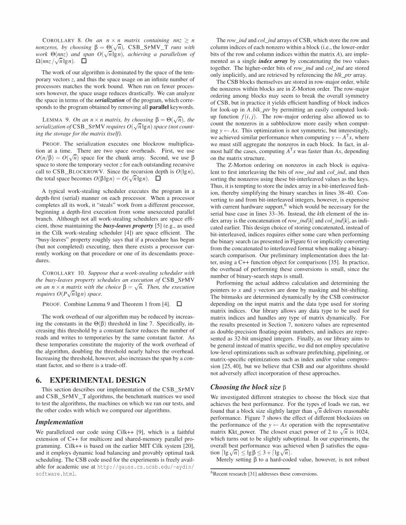
performance. Figure 7 shows the effect of different blocksizes onthe performance of the y← Ax operation with the representativematrix Kkt_power. The closest exact power of 2 to

√n is 1024,

which turns out to be slightly suboptimal. In our experiments, theoverall best performance was achieved when β satisfies the equa-tion ⌈lg√n⌉ ≤ lgβ≤ 3+⌈lg√n⌉.

Merely setting β to a hard-coded value, however, is not robust

6Recent research [31] addresses these conversions.

0

100

200

300

400

500

32 64

128 256

512 1024

2048 4096

8192 16384

32768

MF

lops

/sec

Block size

p=8p=4p=2

7: The effect of block size parameter β on SpMV performance using theKkt_power matrix. For values β > 32768 and β < 32, the experiment failedto finish due to memory limitations. The experiment was conducted on theAMD Opteron.

for various reasons. First, the elements stored in the index ar-ray should use the same data type as that used for matrix indices.Specifically, the integer β− 1 should fit in 2 bytes so that a con-catenated row_ind and col_ind fit into 4 bytes. Second, the length-β regions of the input vector x and output vector y (which are ac-cessed when multiplying a single block) should comfortably fit intoL2 cache. Finally, to ensure speedup on matrices with evenly dis-tributed nonzeros, there should be enough parallel slackness forthe parallelization across blockrows (i.e., the highest level paral-lelism). Specifically, when β grows large, the parallelism is roughlybounded by O(nnz/(β lg(n/β))) (by dividing the work and spanfrom Theorem 6). Thus, we want nnz/(β lg(n/β)) to be “largeenough,” which means limiting the maximum magnitude of β.

We adjusted our CSB constructor, therefore, to automaticallyselect a reasonable block-size parameter β. It starts with β =3+ ⌈lg√n⌉ and keeps decreasing it until the aforementioned con-straints are satisfied. Although a research opportunity may exist toautotune the optimal block size with respect to a specific matrix andarchitecture, in most test matrices, choosing β =

√n degraded per-

formance by at most 10%–15%. The optimal β value barely shiftsalong the x-axis when running on different numbers of processorsand is quite stable overall.

An optimization heuristic for structured matrices

Even though CSB_SPMV and CSB_SPMV_T are robust and ex-hibit plenty of parallelism on most matrices, their practical perfor-mance can be improved on some sparse matrices having regularstructure. In particular, a block diagonal matrix with equally sizedblocks has nonzeros that are evenly distributed across blockrows.In this case, a simple algorithm based on blockrow parallelismwould suffice in place of the more complicated recursive methodfrom CSB_BLOCKV. This divide-and-conquer within blockrowsincurs overhead that might unnecessarily degrade performance.Thus, when the nonzeros are evenly distributed across the block-rows, our implementation of the top-level algorithm (given inFigure 4) calls the serial multiplication in line 12 instead of theCSB_BLOCKROWV procedure.

To see whether a given matrix is amenable to the optimization,we apply the following “balance” heuristic. We calculate the imbal-ance among blockrows (or blockcolumns in the case of y← ATx)and apply the optimization only when no blocks have more thantwice the average number of nonzeros per blockrow. In otherwords, if max(nnz(Ai)) < 2 ·mean(nnz(Ai)), then the matrix is con-sidered to have balanced blockrows and the optimization is applied.

Of course, this optimization is not the only way to achieve a per-formance boost on structured matrices.

Optimization of temporary vectors

One of the most significant overheads of our algorithm is the useof temporary vectors to store intermediate results when paralleliz-ing a blockrow multiplication in CSB_BLOCKROWV. The “bal-ance” heuristic above is one way of reducing this overhead whenthe nonzeros in the matrix are evenly distributed. For arbitrarymatrices, however, we can still reduce the overhead in practice.In particular, we only need to allocate the temporary vector z (inline 26) if both of the subsequent multiplications (lines 27–29) arescheduled in parallel. If the first recursive call completes beforethe second recursive call begins, then we instead write directly intothe output vector for both recursive calls. In other words, whena blockrow multiplication is scheduled serially, the multiplicationprocedure detects this fact and mimics a normal serial execution,without the use of temporary vectors. Our implementation exploitsan undocumented feature of Cilk++ to test whether the first call hascompleted before making the second recursive call, and we allocatethe temporary as appropriate. This test may also be implementedusing Cilk++ reducers [19].

Sparse-matrix test suite

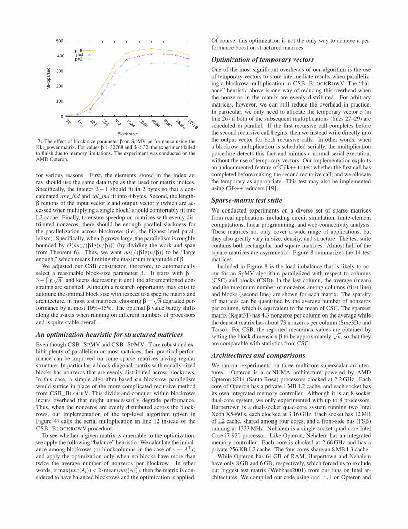
We conducted experiments on a diverse set of sparse matricesfrom real applications including circuit simulation, finite-elementcomputations, linear programming, and web-connectivity analysis.These matrices not only cover a wide range of applications, butthey also greatly vary in size, density, and structure. The test suitecontains both rectangular and square matrices. Almost half of thesquare matrices are asymmetric. Figure 8 summarizes the 14 testmatrices.

Included in Figure 8 is the load imbalance that is likely to oc-cur for an SpMV algorithm parallelized with respect to columns(CSC) and blocks (CSB). In the last column, the average (mean)and the maximum number of nonzeros among columns (first line)and blocks (second line) are shown for each matrix. The sparsityof matrices can be quantified by the average number of nonzerosper column, which is equivalent to the mean of CSC. The sparsestmatrix (Rajat31) has 4.3 nonzeros per column on the average whilethe densest matrix has about 73 nonzeros per column (Sme3Dc andTorso). For CSB, the reported mean/max values are obtained bysetting the block dimension β to be approximately

√n, so that they

are comparable with statistics from CSC.

Architectures and comparisons

We ran our experiments on three multicore superscalar architec-tures. Opteron is a ccNUMA architecture powered by AMDOpteron 8214 (Santa Rosa) processors clocked at 2.2 GHz. Eachcore of Opteron has a private 1 MB L2 cache, and each socket hasits own integrated memory controller. Although it is an 8-socketdual-core system, we only experimented with up to 8 processors.Harpertown is a dual-socket quad-core system running two IntelXeon X5460’s, each clocked at 3.16 GHz. Each socket has 12 MBof L2 cache, shared among four cores, and a front-side bus (FSB)running at 1333 MHz. Nehalem is a single-socket quad-core IntelCore i7 920 processor. Like Opteron, Nehalem has an integratedmemory controller. Each core is clocked at 2.66 GHz and has aprivate 256 KB L2 cache. The four cores share an 8 MB L3 cache.

While Opteron has 64 GB of RAM, Harpertown and Nehalemhave only 8 GB and 6 GB, respectively, which forced us to excludeour biggest test matrix (Webbase2001) from our runs on Intel ar-chitectures. We compiled our code using gcc 4.1 on Opteron and

Name

Spy Plot

Dimensions CSC (mean/max)

Description Nonzeros CSB (mean/max)

Asic_320k 321K×321K 6.0 / 157K

circuit simulation 1,931K 4.9 / 2.3K

Sme3Dc 42K×42K 73.3 / 405

3D structural 3,148K 111.6 / 1368

mechanics

Parabolic_fem 525K×525K 7.0 / 7

diff-convection 3,674K 3.5 / 1,534

reaction

Mittelmann 1,468K×1,961K 2.7 / 7

LP problem 5,382K 2.0 / 3,713

Rucci 1,977K×109K 70.9 / 108

Ill-conditioned 7,791K 9.4 / 36

least-squares

Torso 116K×116K 73.3 / 1.2K

Finite diff, 8,516K 41.3 / 36.6K

2D model of torso

Kkt_power 2.06M×2.06M 6.2 / 90

optimal power flow, 12.77M 3.1 / 1,840

nonlinear opt.

Rajat31 4.69M×4.69M 4.3 / 1.2K

circuit simulation 20.31M 3.9 / 8.7K

Ldoor 952K×952K 44.6 / 77

structural prob. 42.49M 49.1 / 43,872

Bone010 986K×986K 48.5 / 63

3D trabecular bone 47.85M 51.5 / 18,670

Grid3D200 8M×8M 6.97 / 7

3D 7-point 55.7M 3.7 / 9,818

finite-diff mesh

RMat23 8.4M×8.4M 9.4 / 70.3K

Real-world 78.7M 4.7 / 222.1K

graph model

Cage15 5.15M×5.15M 19.2 / 47

DNA electrophoresis 99.2M 15.6 / 39,712

Webbase2001 118M×118M 8.6 / 816K

Web connectivity 1,019M 4.9 / 2,375K

8: Structural information on the sparse matrices used in our experiments,ordered by increasing number of nonzeros. The first ten matrices andCage15 are from the University of Florida sparse matrix collection [12].Grid3D200 is a 7-point finite difference mesh generated using the MatlabMesh Partitioning and Graph Separator Toolbox [22]. The RMat23 ma-trix [26], which models scale-free graphs, is generated by using repeatedKronecker products [2]. We chose parameters A = 0.7, B = C = D = 0.1for RMat23 in order to generate skewed matrices. Webbase2001 is a crawlof the World Wide Web from the year 2001 [8].

0

100

200

300

400

500

600

700

Asic_320k

Sme3Dc

Parabolic_fem

Mittelm

ann

Rucci

TorsoKkt_power

MF

lops

/sec

p=1p=2p=4p=8

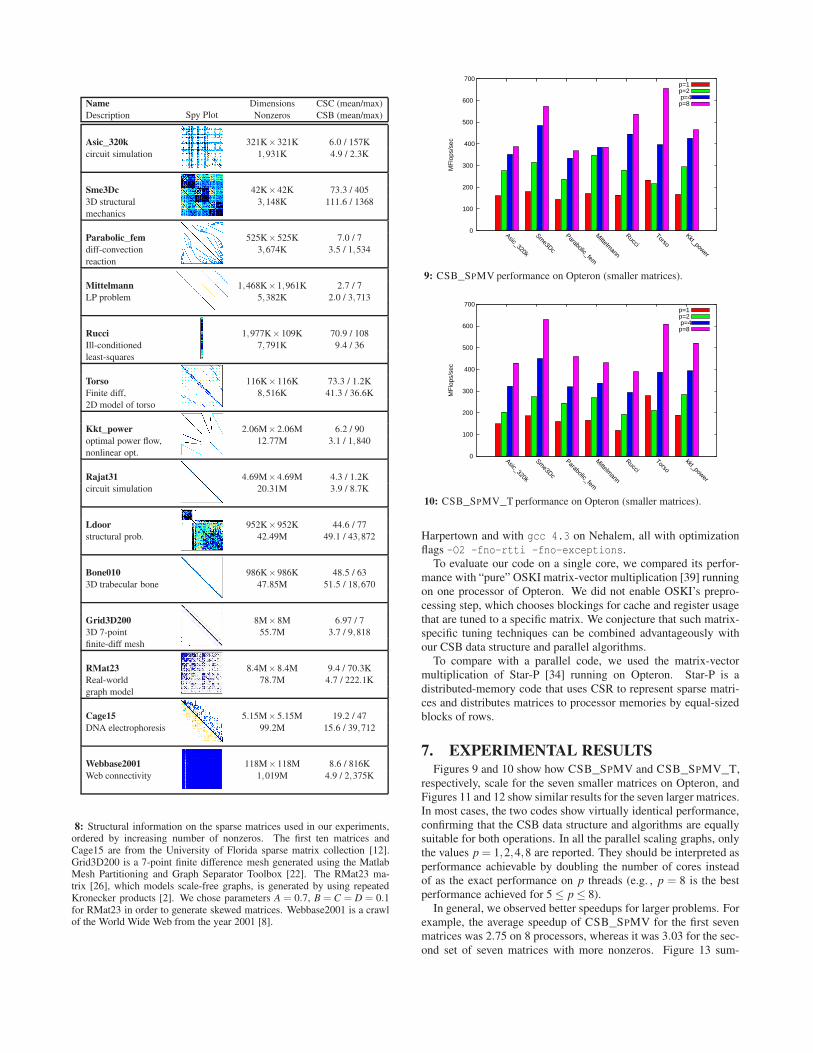
9: CSB_SPMV performance on Opteron (smaller matrices).

0

100

200

300

400

500

600

700

Asic_320k

Sme3Dc

Parabolic_fem

Mittelm

ann

Rucci

Torsokkt_power

MF

lops

/sec

p=1p=2p=4p=8

10: CSB_SPMV_T performance on Opteron (smaller matrices).

Harpertown and with gcc 4.3 on Nehalem, all with optimizationflags -O2 -fno-rtti -fno-exceptions.

To evaluate our code on a single core, we compared its perfor-mance with “pure” OSKI matrix-vector multiplication [39] runningon one processor of Opteron. We did not enable OSKI’s prepro-cessing step, which chooses blockings for cache and register usagethat are tuned to a specific matrix. We conjecture that such matrix-specific tuning techniques can be combined advantageously withour CSB data structure and parallel algorithms.

To compare with a parallel code, we used the matrix-vectormultiplication of Star-P [34] running on Opteron. Star-P is adistributed-memory code that uses CSR to represent sparse matri-ces and distributes matrices to processor memories by equal-sizedblocks of rows.

7. EXPERIMENTAL RESULTSFigures 9 and 10 show how CSB_SPMV and CSB_SPMV_T,

respectively, scale for the seven smaller matrices on Opteron, andFigures 11 and 12 show similar results for the seven larger matrices.In most cases, the two codes show virtually identical performance,confirming that the CSB data structure and algorithms are equallysuitable for both operations. In all the parallel scaling graphs, onlythe values p = 1,2,4,8 are reported. They should be interpreted asperformance achievable by doubling the number of cores insteadof as the exact performance on p threads (e.g. , p = 8 is the bestperformance achieved for 5≤ p≤ 8).

In general, we observed better speedups for larger problems. Forexample, the average speedup of CSB_SPMV for the first sevenmatrices was 2.75 on 8 processors, whereas it was 3.03 for the sec-ond set of seven matrices with more nonzeros. Figure 13 sum-

0

100

200

300

400

500

600

700

Rajat31

Ldoor

Grid3D200

Cage15

RMat23

Bone010

Webbase2001

MF

lops

/sec

p=1p=2p=4p=8

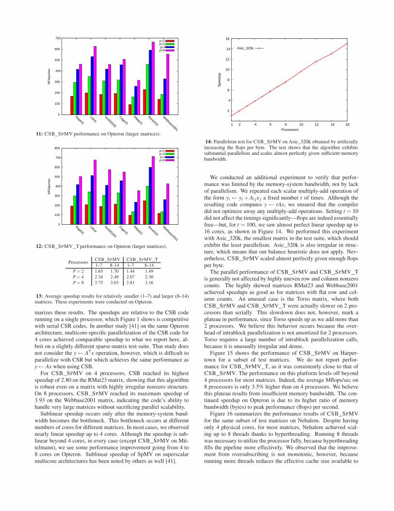
11: CSB_SPMV performance on Opteron (larger matrices).

0

100

200

300

400

500

600

700

800

Rajat31

Ldoor

Grid3D200

Cage15

RMat23

Bone010

Webbase2001

MF

lops

/sec

p=1p=2p=4p=8

12: CSB_SPMV_T performance on Opteron (larger matrices).

ProcessorsCSB_SPMV CSB_SPMV_T

1–7 8–14 1–7 8–14

P = 2 1.65 1.70 1.44 1.49

P = 4 2.34 2.49 2.07 2.30

P = 8 2.75 3.03 2.81 3.16

13: Average speedup results for relatively smaller (1–7) and larger (8–14)matrices. These experiments were conducted on Opteron.

marizes these results. The speedups are relative to the CSB coderunning on a single processor, which Figure 1 shows is competitivewith serial CSR codes. In another study [41] on the same Opteronarchitecture, multicore-specific parallelization of the CSR code for4 cores achieved comparable speedup to what we report here, al-beit on a slightly different sparse-matrix test suite. That study doesnot consider the y← ATx operation, however, which is difficult toparallelize with CSR but which achieves the same performance asy← Ax when using CSB.

For CSB_SPMV on 4 processors, CSB reached its highestspeedup of 2.80 on the RMat23 matrix, showing that this algorithmis robust even on a matrix with highly irregular nonzero structure.On 8 processors, CSB_SPMV reached its maximum speedup of3.93 on the Webbase2001 matrix, indicating the code’s ability tohandle very large matrices without sacrificing parallel scalability.

Sublinear speedup occurs only after the memory-system band-width becomes the bottleneck. This bottleneck occurs at differentnumbers of cores for different matrices. In most cases, we observednearly linear speedup up to 4 cores. Although the speedup is sub-linear beyond 4 cores, in every case (except CSB_SPMV on Mit-telmann), we see some performance improvement going from 4 to8 cores on Opteron. Sublinear speedup of SpMV on superscalarmulticore architectures has been noted by others as well [41].

2

4

6

8

10

12

14

16

1 2 4 6 8 10 12 14 16

Spe

edup

Processors

Asic_320k

14: Parallelism test for CSB_SPMV on Asic_320k obtained by artificiallyincreasing the flops per byte. The test shows that the algorithm exhibitssubstantial parallelism and scales almost perfectly given sufficient memorybandwidth.

We conducted an additional experiment to verify that perfor-mance was limited by the memory-system bandwidth, not by lackof parallelism. We repeated each scalar multiply-add operation ofthe form yi ← yi + Ai jx j a fixed number t of times. Although theresulting code computes y ← tAx, we ensured that the compilerdid not optimize away any multiply-add operations. Setting t = 10did not affect the timings significantly—flops are indeed essentiallyfree—but, for t = 100, we saw almost perfect linear speedup up to16 cores, as shown in Figure 14. We performed this experimentwith Asic_320k, the smallest matrix in the test suite, which shouldexhibit the least parallelism. Asic_320k is also irregular in struc-ture, which means that our balance heuristic does not apply. Nev-ertheless, CSB_SPMV scaled almost perfectly given enough flopsper byte.

The parallel performance of CSB_SPMV and CSB_SPMV_Tis generally not affected by highly uneven row and column nonzerocounts. The highly skewed matrices RMat23 and Webbase2001achieved speedups as good as for matrices with flat row and col-umn counts. An unusual case is the Torso matrix, where bothCSB_SPMV and CSB_SPMV_T were actually slower on 2 pro-cessors than serially. This slowdown does not, however, mark aplateau in performance, since Torso speeds up as we add more than2 processors. We believe this behavior occurs because the over-head of intrablock parallelization is not amortized for 2 processors.Torso requires a large number of intrablock parallelization calls,because it is unusually irregular and dense.

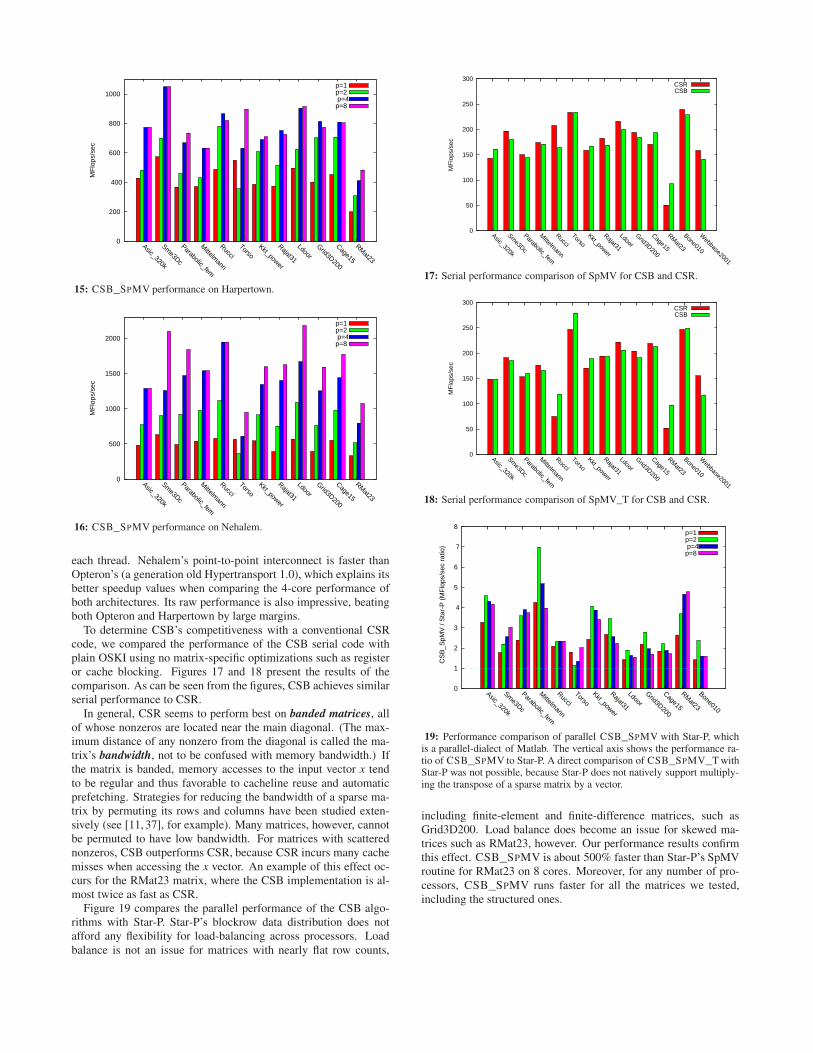
Figure 15 shows the performance of CSB_SPMV on Harper-town for a subset of test matrices. We do not report perfor-mance for CSB_SPMV_T, as it was consistently close to that ofCSB_SPMV. The performance on this platform levels off beyond4 processors for most matrices. Indeed, the average Mflops/sec on8 processors is only 3.5% higher than on 4 processors. We believethis plateau results from insufficient memory bandwidth. The con-tinued speedup on Opteron is due to its higher ratio of memorybandwidth (bytes) to peak performance (flops) per second.

Figure 16 summarizes the performance results of CSB_SPMVfor the same subset of test matrices on Nehalem. Despite havingonly 4 physical cores, for most matrices, Nehalem achieved scal-ing up to 8 threads thanks to hyperthreading. Running 8 threadswas necessary to utilize the processor fully, because hyperthreadingfills the pipeline more effectively. We observed that the improve-ment from oversubscribing is not monotonic, however, becauserunning more threads reduces the effective cache size available to

0

200

400

600

800

1000

Asic_320k

Sme3Dc

Parabolic_fem

Mittelm

ann

Rucci

TorsoKkt_power

Rajat31

Ldoor

Grid3D200

Cage15

RMat23

MF

lops

/sec

p=1p=2p=4

p=8

15: CSB_SPMV performance on Harpertown.

0

500

1000

1500

2000

Asic_320k

Sme3Dc

Parabolic_fem

Mittelm

ann

Rucci

TorsoKkt_power

Rajat31

Ldoor

Grid3D200

Cage15

RMat23

MF

lops

/sec

p=1p=2p=4

p=8

16: CSB_SPMV performance on Nehalem.

each thread. Nehalem’s point-to-point interconnect is faster thanOpteron’s (a generation old Hypertransport 1.0), which explains itsbetter speedup values when comparing the 4-core performance ofboth architectures. Its raw performance is also impressive, beatingboth Opteron and Harpertown by large margins.

To determine CSB’s competitiveness with a conventional CSRcode, we compared the performance of the CSB serial code withplain OSKI using no matrix-specific optimizations such as registeror cache blocking. Figures 17 and 18 present the results of thecomparison. As can be seen from the figures, CSB achieves similarserial performance to CSR.

In general, CSR seems to perform best on banded matrices, allof whose nonzeros are located near the main diagonal. (The max-imum distance of any nonzero from the diagonal is called the ma-trix’s bandwidth, not to be confused with memory bandwidth.) Ifthe matrix is banded, memory accesses to the input vector x tendto be regular and thus favorable to cacheline reuse and automaticprefetching. Strategies for reducing the bandwidth of a sparse ma-trix by permuting its rows and columns have been studied exten-sively (see [11, 37], for example). Many matrices, however, cannotbe permuted to have low bandwidth. For matrices with scatterednonzeros, CSB outperforms CSR, because CSR incurs many cachemisses when accessing the x vector. An example of this effect oc-curs for the RMat23 matrix, where the CSB implementation is al-most twice as fast as CSR.

Figure 19 compares the parallel performance of the CSB algo-rithms with Star-P. Star-P’s blockrow data distribution does notafford any flexibility for load-balancing across processors. Loadbalance is not an issue for matrices with nearly flat row counts,

0

50

100

150

200

250

300

Asic_320k

Sme3Dc

Parabolic_fem

Mittelm

ann

Rucci

TorsoKkt_power

Rajat31

Ldoor

Grid3D200

Cage15

RMat23

Bone010

Webbase2001

MF

lops

/sec

CSRCSB

17: Serial performance comparison of SpMV for CSB and CSR.

0

50

100

150

200

250

300

Asic_320k

Sme3Dc

Parabolic_fem

Mittelm

ann

Rucci

TorsoKkt_power

Rajat31

Ldoor

Grid3D200

Cage15

RMat23

Bone010

Webbase2001

MF

lops

/sec

CSRCSB

18: Serial performance comparison of SpMV_T for CSB and CSR.

0

1

2

3

4

5

6

7

8

Asic_320k

Sme3Dc

Parabolic_fem

Mittelm

ann

Rucci

TorsoKkt_power

Rajat31

Ldoor

Grid3D200

Cage15

RMat23

Bone010

CS

B_S

pMV

/ S

tar-

P (

MF

lops

/sec

rat

io)

p=1p=2p=4

p=8

19: Performance comparison of parallel CSB_SPMV with Star-P, whichis a parallel-dialect of Matlab. The vertical axis shows the performance ra-tio of CSB_SPMV to Star-P. A direct comparison of CSB_SPMV_T withStar-P was not possible, because Star-P does not natively support multiply-ing the transpose of a sparse matrix by a vector.

including finite-element and finite-difference matrices, such asGrid3D200. Load balance does become an issue for skewed ma-trices such as RMat23, however. Our performance results confirmthis effect. CSB_SPMV is about 500% faster than Star-P’s SpMVroutine for RMat23 on 8 cores. Moreover, for any number of pro-cessors, CSB_SPMV runs faster for all the matrices we tested,including the structured ones.

8. CONCLUSIONCompressed sparse blocks allow parallel operations on sparse

matrices to proceed either row-wise or column-wise with equal fa-cility. We have demonstrated the efficacy of the CSB storage for-mat for SpMV calculations on a sparse matrix or its transpose. Itremains to be seen, however, whether the CSB format is limitedto SpMV calculations or if it can also be effective in enabling par-allel algorithms for multiplying two sparse matrices, performingLU-, LUP-, and related decompositions, linear programming, anda host of other problems for which serial sparse-matrix algorithmscurrently use the CSC and CSR storage formats.

The CSB format readily enables parallel SpMV calculations ona symmetric matrix where only half the matrix is stored, but wewere unable to attain one optimization that serial codes exploitin this situation. In a typical serial code that computes y← Ax,where A = (ai j) is a symmetric matrix, when a processor fetchesai j = a ji out of memory to perform the update yi ← yi + ai jx j,it can also perform the update y j ← y j + ai jxi at the same time.This strategy halves the memory bandwidth compared to execut-ing CSB_SPMV on the matrix, where ai j = a ji is fetched twice.It remains an open problem whether the 50% savings in storagefor sparse matrices can be coupled with a 50% savings in memorybandwidth, which is an important factor of 2, since it appears thatthe bandwidth between multicore chips and DRAM will scale moreslowly than core count.

9. REFERENCES

[1] M. D. Adams and D. S. Wise. Seven at one stroke: results from acache-oblivious paradigm for scalable matrix algorithms. In MSPC,pages 41–50, New York, NY, USA, 2006. ACM.

[2] D. Bader, J. Feo, J. Gilbert, J. Kepner, D. Koester, E. Loh,K. Madduri, B. Mann, and T. Meuse. HPCS scalable syntheticcompact applications #2. Version 1.1.

[3] G. E. Blelloch. Programming parallel algorithms. CACM, 39(3), Mar.1996.

[4] R. D. Blumofe, C. F. Joerg, B. C. Kuszmaul, C. E. Leiserson, K. H.Randall, and Y. Zhou. Cilk: An efficient multithreaded runtimesystem. In PPoPP, pages 207–216, Santa Barbara, CA, July 1995.

[5] R. D. Blumofe and C. E. Leiserson. Scheduling multithreadedcomputations by work stealing. JACM, 46(5):720–748, Sept. 1999.

[6] A. Buluç and J. R. Gilbert. On the representation and multiplicationof hypersparse matrices. In IPDPS, pages 1–11, 2008.

[7] U. Catalyurek and C. Aykanat. A fine-grain hypergraph model for 2Ddecomposition of sparse matrices. In IPDPS, page 118, Washington,DC, USA, 2001. IEEE Computer Society.

[8] J. Cho, H. Garcia-Molina, T. Haveliwala, W. Lam, A. Paepcke,S. Raghavan, and G. Wesley. Stanford webbase components andapplications. ACM Transactions on Internet Technology,6(2):153–186, 2006.

[9] Cilk Arts, Inc., Burlington, MA. Cilk++ Programmer’s Guide, 2009.Available from http://www.cilk.com/.

[10] T. H. Cormen, C. E. Leiserson, R. L. Rivest, and C. Stein.Introduction to Algorithms. The MIT Press, third edition, 2009.

[11] E. Cuthill and J. McKee. Reducing the bandwidth of sparsesymmetric matrices. In Proceedings of the 24th National Conference,pages 157–172, New York, NY, USA, 1969. ACM.

[12] T. A. Davis. University of Florida sparse matrix collection. NADigest, 92, 1994.

[13] T. A. Davis. Direct Methods for Sparse Linear Systems. SIAM,Philadelpha, PA, 2006.

[14] J. Dongarra. Sparse matrix storage formats. In Z. Bai, J. Demmel,J. Dongarra, A. Ruhe, and H. van der Vorst, editors, Templates for theSolution of Algebraic Eigenvalue Problems: a Practical Guide.SIAM, 2000.

[15] J. Dongarra, P. Koev, and X. Li. Matrix-vector and matrix-matrixmultiplication. In Z. Bai, J. Demmel, J. Dongarra, A. Ruhe, andH. van der Vorst, editors, Templates for the Solution of AlgebraicEigenvalue Problems: a Practical Guide. SIAM, 2000.

[16] I. S. Duff, A. M. Erisman, and J. K. Reid. Direct Methods for SparseMatrices. Oxford University Press, New York, 1986.

[17] S. C. Eisenstat, M. C. Gursky, M. H. Schultz, and A. H. Sherman.Yale sparse matrix package I: The symmetric codes. InternationalJournal for Numerical Methods in Engineering, 18:1145–1151,1982.

[18] E. Elmroth, F. Gustavson, I. Jonsson, and B. Kågström. Recursiveblocked algorithms and hybrid data structures for dense matrixlibrary software. SIAM Review, 46(1):3–45, 2004.

[19] M. Frigo, P. Halpern, C. E. Leiserson, and S. Lewin-Berlin. Reducersand other Cilk++ hyperobjects. In SPAA, Calgary, Canada, 2009.

[20] M. Frigo, C. E. Leiserson, and K. H. Randall. The implementation ofthe Cilk-5 multithreaded language. In SIGPLAN, pages 212–223,Montreal, Quebec, Canada, June 1998.

[21] A. George and J. W. Liu. Computer Solution of Sparse PositiveDefinite Systems. Prentice-Hall, Englewood Cliffs, NJ, 1981.

[22] J. R. Gilbert, G. L. Miller, and S.-H. Teng. Geometric meshpartitioning: Implementation and experiments. SIAM Journal onScientific Computing, 19(6):2091–2110, 1998.

[23] J. R. Gilbert, C. Moler, and R. Schreiber. Sparse matrices inMATLAB: Design and implementation. SIAM J. Matrix Anal. Appl,13:333–356, 1991.

[24] E.-J. Im, K. Yelick, and R. Vuduc. Sparsity: Optimization frameworkfor sparse matrix kernels. International Journal of High PerformanceComputing Applications, 18(1):135–158, 2004.

[25] K. Kourtis, G. Goumas, and N. Koziris. Optimizing sparsematrix-vector multiplication using index and value compression. InComputing Frontiers (CF), pages 87–96, New York, NY, USA, 2008.ACM.

[26] J. Leskovec, D. Chakrabarti, J. M. Kleinberg, and C. Faloutsos.Realistic, mathematically tractable graph generation and evolution,using Kronecker multiplication. In PKDD, pages 133–145, 2005.

[27] K. P. Lorton and D. S. Wise. Analyzing block locality inMorton-order and Morton-hybrid matrices. SIGARCH ComputerArchitecture News, 35(4):6–12, 2007.

[28] H. M. Markowitz. The elimination form of the inverse and itsapplication to linear programming. Management Science,3(3):255–269, 1957.

[29] G. Morton. A computer oriented geodetic data base and a newtechnique in file sequencing. Technical report, IBM Ltd., Ottawa,Canada, Mar. 1966.

[30] R. Nishtala, R. W. Vuduc, J. W. Demmel, and K. A. Yelick. Whencache blocking of sparse matrix vector multiply works and why.Applicable Algebra in Engineering, Communication and Computing,18(3):297–311, 2007.

[31] R. Raman and D. S. Wise. Converting to and from dilated integers.IEEE Trans. on Computers, 57(4):567–573, 2008.

[32] Y. Saad. Iterative Methods for Sparse Linear Systems. SIAM,Philadelpha, PA, second edition, 2003.

[33] N. Sato and W. F. Tinney. Techniques for exploiting the sparsity ofthe network admittance matrix. IEEE Trans. Power Apparatus andSystems, 82(69):944–950, Dec. 1963.

[34] V. Shah and J. R. Gilbert. Sparse matrices in Matlab*P: Design andimplementation. In HiPC, pages 144–155, 2004.

[35] B. Stroustrup. The C++ Programming Language. Addison-Wesley,third edition, 2000.

[36] W. Tinney and J. Walker. Direct solutions of sparse networkequations by optimally ordered triangular factorization. Proceedingsof the IEEE, 55(11):1801–1809, Nov. 1967.

[37] S. Toledo. Improving the memory-system performance ofsparse-matrix vector multiplication. IBM J. Research andDevelopment, 41(6):711–726, 1997.

[38] B. Vastenhouw and R. H. Bisseling. A two-dimensional datadistribution method for parallel sparse matrix-vector multiplication.SIAM Rev., 47(1):67–95, 2005.

[39] R. Vuduc, J. W. Demmel, and K. A. Yelick. OSKI: A library ofautomatically tuned sparse matrix kernels. Journal of Physics:Conference Series, 16(1):521+, 2005.

[40] J. Willcock and A. Lumsdaine. Accelerating sparse matrixcomputations via data compression. In ICS, pages 307–316, NewYork, NY, USA, 2006. ACM.

[41] S. Williams, L. Oliker, R. Vuduc, J. Shalf, K. Yelick, and J. Demmel.Optimization of sparse matrix-vector multiplication on emergingmulticore platforms. Parallel Computing, 35(3):178–194, 2009.