MATRIX MULTIVARIATE PEARSON II-RIESZ DISTRIBUTIONrepo.risat.org/262/1/2015-3.pdfalbanian journal of mathematics volume9,number1,pages63–75 issn: 1930-1235;(2015) matrix multivariate

ALBANIAN JOURNAL OF MATHEMATICSVolume 9, Number 1, Pages 63–75ISSN: 1930-1235; (2015)

MATRIX MULTIVARIATE PEARSON II-RIESZ DISTRIBUTION

José A. Díaz-GarcíaUniversidad Autónoma Agraria Antonio Narro,Calzada Antonio Narro 1923, Col. Buenavista,

25315 Saltillo, Coahuila, MéxicoEmail: [email protected]

Ramón Gutiérrez-SánchezDepartment of Statistics and O.R,

University of Granada,Granada 18071, SpainEmail: [email protected]

Abstract. Matrix multivariate Pearson type II-Riesz distribution is definedand some of its properties are studied. In particular, the associated matrixmultivariate beta distribution type I is derived. Also the singular values andeigenvalues distributions are obtained.

1. Introduction

When a new statistic theory is proposed, the statistician known well about therigorously mathematical foundations of their discipline, however in order to reacha wider interdisciplinary public, some of the classical statistical techniques havebeen usually published without explaining the supporting abstract mathematicaltools which governs the approach. For example, in the context of the distributiontheory of random matrices, in the last 20 years, a number of more abstract andmathematical approaches have emerged for studying and generalizing the usualmatrix variate distributions. In particular, this needing have appeared recentlyin the generalization, by using abstract algebra, of some results of real randommatrices to another supporting fields, such as complex, quaternion and octonion,see [26], [27], [12], [15], among many others authors. Studying distribution theoryby another algebras, beyond real, have led several generalizations of substantialunderstanding in the theoretical context, and we expect that it is more extensivelyapplied when a an improvement of its unified potential can be explored in other

2010 Mathematics Subject Classification. Primary 60E05; 15A52; 15B33; Secondary 15A09;15B52; 62E15;Key words and phrases. Matrix multivariate; Pearson Type II distribution; Riesz distribution;Kotz-Riesz distribution; real, complex,quaternion and octonion random matrices; real normeddivision algebras.

c©2015 albanian-j-math.com

63

http://albanian-j-math.com

Albanian J. Math. 9 (2015), no. 1, 63-75.

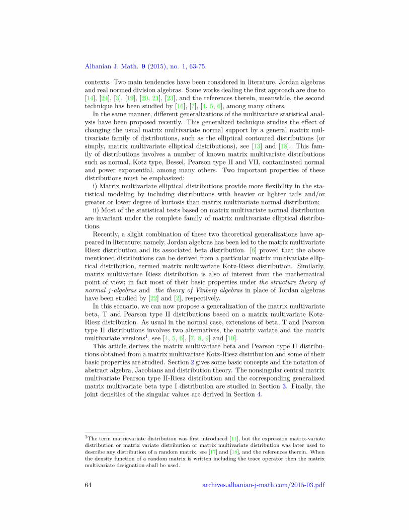
contexts. Two main tendencies have been considered in literature, Jordan algebrasand real normed division algebras. Some works dealing the first approach are due to[14], [24], [3], [19], [20, 21], [23], and the references therein, meanwhile, the secondtechnique has been studied by [16], [7], [4, 5, 6], among many others.

In the same manner, different generalizations of the multivariate statistical anal-ysis have been proposed recently. This generalized technique studies the effect ofchanging the usual matrix multivariate normal support by a general matrix mul-tivariate family of distributions, such as the elliptical contoured distributions (orsimply, matrix multivariate elliptical distributions), see [13] and [18]. This fam-ily of distributions involves a number of known matrix multivariate distributionssuch as normal, Kotz type, Bessel, Pearson type II and VII, contaminated normaland power exponential, among many others. Two important properties of thesedistributions must be emphasized:

i) Matrix multivariate elliptical distributions provide more flexibility in the sta-tistical modeling by including distributions with heavier or lighter tails and/orgreater or lower degree of kurtosis than matrix multivariate normal distribution;

ii) Most of the statistical tests based on matrix multivariate normal distributionare invariant under the complete family of matrix multivariate elliptical distribu-tions.

Recently, a slight combination of these two theoretical generalizations have ap-peared in literature; namely, Jordan algebras has been led to the matrix multivariateRiesz distribution and its associated beta distribution. [6] proved that the abovementioned distributions can be derived from a particular matrix multivariate ellip-tical distribution, termed matrix multivariate Kotz-Riesz distribution. Similarly,matrix multivariate Riesz distribution is also of interest from the mathematicalpoint of view; in fact most of their basic properties under the structure theory ofnormal j-algebras and the theory of Vinberg algebras in place of Jordan algebrashave been studied by [22] and [2], respectively.

In this scenario, we can now propose a generalization of the matrix multivariatebeta, T and Pearson type II distributions based on a matrix multivariate Kotz-Riesz distribution. As usual in the normal case, extensions of beta, T and Pearsontype II distributions involves two alternatives, the matrix variate and the matrixmultivariate versions1, see [4, 5, 6], [7, 8, 9] and [10].

This article derives the matrix multivariate beta and Pearson type II distribu-tions obtained from a matrix multivariate Kotz-Riesz distribution and some of theirbasic properties are studied. Section 2 gives some basic concepts and the notation ofabstract algebra, Jacobians and distribution theory. The nonsingular central matrixmultivariate Pearson type II-Riesz distribution and the corresponding generalizedmatrix multivariate beta type I distribution are studied in Section 3. Finally, thejoint densities of the singular values are derived in Section 4.

1The term matricvariate distribution was first introduced [11], but the expression matrix-variatedistribution or matrix variate distribution or matrix multivariate distribution was later used todescribe any distribution of a random matrix, see [17] and [18], and the references therein. Whenthe density function of a random matrix is written including the trace operator then the matrixmultivariate designation shall be used.

64 archives.albanian-j-math.com/2015-03.pdf


http://archives.albanian-j-math.com/2015-03.pdf


2. Preliminary results

A detailed discussion of real normed division algebras can be found in [1] and[25]. For your convenience, we shall introduce some notation, although in general,we adhere to standard notation forms.

For our purposes: Let F be a field. An algebra A over F is a pair (A;m), whereA is a finite-dimensional vector space over F and multiplication m : A × A → A isan F-bilinear map; that is, for all λ ∈ F, x, y, z ∈ A,

m(x, λy + z) = λm(x; y) +m(x; z)m(λx+ y; z) = λm(x; z) +m(y; z).

Two algebras (A;m) and (E;n) over F are said to be isomorphic if there is aninvertible map φ : A→ E such that for all x, y ∈ A,

φ(m(x, y)) = n(φ(x), φ(y)).

By simplicity, we write m(x; y) = xy for all x, y ∈ A.Let A be an algebra over F. Then A is said to be(1) alternative if x(xy) = (xx)y and x(yy) = (xy)y for all x, y ∈ A,(2) associative if x(yz) = (xy)z for all x, y, z ∈ A,(3) commutative if xy = yx for all x, y ∈ A, and(4) unital if there is a 1 ∈ A such that x1 = x = 1x for all x ∈ A.If A is unital, then the identity 1 is uniquely determined.An algebra A over F is said to be a division algebra if A is nonzero and xy =

0A ⇒ x = 0A or y = 0A for all x, y ∈ A.The term “division algebra", comes from the following proposition, which shows

that, in such an algebra, left and right division can be unambiguously performed.Let A be an algebra over F. Then A is a division algebra if, and only if, A is

nonzero and for all a, b ∈ A, with b 6= 0A, the equations bx = a and yb = a haveunique solutions x, y ∈ A.

In the sequel we assume F = < and consider classes of division algebras over <or “real division algebras" for short.

We introduce the algebras of real numbers <, complex numbers C, quaternionsH and octonions O. Then, if A is an alternative real division algebra, then A isisomorphic to <, C, H or O.

Let A be a real division algebra with identity 1. Then A is said to be normed ifthere is an inner product (·, ·) on A such that

(xy, xy) = (x, x)(y, y) for all x, y ∈ A.

If A is a real normed division algebra, then A is isomorphic <, C, H or O.There are exactly four normed division algebras: real numbers (<), complex

numbers (C), quaternions (H) and octonions (O), see [1]. We take into accountthat should be taken into account, <, C, H and O are the only normed divisionalgebras; furthermore, they are the only alternative division algebras.

Let A be a division algebra over the real numbers. Then A has dimension either1, 2, 4 or 8. Finally, observe that< is a real commutative associative normed division algebra,C is a commutative associative normed division algebra,H is an associative normed division algebra,O is an alternative normed division algebra.

archives.albanian-j-math.com/2015-03.pdf 65




Let Lβn,m be the set of all n×m matrices of rank m ≤ n over A with m distinctpositive singular values, where A denotes a real finite-dimensional normed divisionalgebra. Let An×m be the set of all n × m matrices over A. The dimension ofAn×m over < is βmn. Let A ∈ An×m, then A∗ = AT denotes the usual conjugatetranspose.

Table 1 sets out the equivalence between the same concepts in the four normeddivision algebras.

Table 1. Notation

Real Complex Quaternion Octonion Genericnotation

Semi-orthogonal Semi-unitary Semi-symplectic Semi-exceptionaltype Vβm,n

Orthogonal Unitary Symplectic Exceptionaltype Uβ(m)

Symmetric Hermitian Quaternionhermitian

Octonionhermitian Sβm

We denote by Sβm the real vector space of all S ∈ Am×m such that S = S∗. In

addition, let Pβm be the cone of positive definite matrices S ∈ Am×m. Thus, Pβ

m

consist of all matrices S = X∗X, with X ∈ Lβn,m; then Pβm is an open subset of

Sβm.Let Dβ

m consisting of all D ∈ Am×m, D = diag(d1, . . . , dm). Let TβU (m) bethe subgroup of all upper triangular matrices T ∈ Am×m such that tij = 0 for1 < i < j ≤ m. Let Z ∈ Lβn,m, define the norm of Z as ||Z|| =

√tr Z∗Z.

For any matrix X ∈ An×m, dX denotes the matrix of differentials (dxij). Finally,we define the measure or volume element (dX) when X ∈ An×m,Sβ

m, Dβm or Vβm,n,

see [7] and [9].If X ∈ An×m then (dX) (the Lebesgue measure in An×m) denotes the exterior

product of the βmn functionally independent variables

(dX) =n∧i=1

m∧j=1

dxij where dxij =β∧k=1

dx(k)ij .

If S ∈ Sβm (or S ∈ TβU (m) with tii > 0, i = 1, . . . ,m) then (dS) (the Lebesgue

measure in Sβm or in TβU (m)) denotes the exterior product of the exterior product

of the m(m− 1)β/2 +m functionally independent variables,

(dS) =m∧i=1

dsii

m∧i>j

β∧k=1

ds(k)ij .

Observe, that for the Lebesgue measure (dS) defined thus, it is required that S ∈Pβm, that is, S must be a non singular Hermitian matrix (Hermitian definite positive

matrix).If Λ ∈ Dβ

m then (dΛ) (the Legesgue measure inDβm) denotes the exterior product

of the βm functionally independent variables

(dΛ) =n∧i=1

β∧k=1

dλ(k)i .





If H1 ∈ Vβm,n then

(H∗1dH1) =m∧i=1

n∧j=i+1

h∗jdhi.

where H = (H∗1|H∗2)∗ = (h1, . . . ,hm|hm+1, . . . ,hn)∗ ∈ Uβ(n). It can be provedthat this differential form does not depend on the choice of the H2 matrix. Whenn = 1; Vβm,1 defines the unit sphere in Am. This is, of course, an (m − 1)β-dimensional surface in Am. When n = m and denoting H1 by H, (HdH∗) istermed the Haar measure on Uβ(m).

The surface area or volume of the Stiefel manifold Vβm,n is

(1) Vol(Vβm,n) =∫

H1∈Vβm,n(H1dH∗1) = 2mπmnβ/2

Γβm[nβ/2],

where Γβm[a] denotes the multivariate Gamma function for the space Sβm and is

defined as

Γβm[a] =∫

A∈Pβmetr{−A}|A|a−(m−1)β/2−1(dA)

= πm(m−1)β/4m∏i=1

Γ[a− (i− 1)β/2],

and Re(a) > (m−1)β/2. This can be obtained as a particular case of the generalizedgamma function of weight κ for the space Sβ

m with κ = (k1, k2, . . . , km) ∈ <m,taking κ = (0, 0, . . . , 0) ∈ <m and which for Re(a) ≥ (m − 1)β/2 − km is definedby, see [16] and [14],

Γβm[a, κ] =∫

A∈Pβmetr{−A}|A|a−(m−1)β/2−1qκ(A)(dA)(2)

= πm(m−1)β/4m∏i=1

Γ[a+ ki − (i− 1)β/2]

= [a]βκΓβm[a],(3)

where etr(·) = exp(tr(·)), | · | denotes the determinant, and for A ∈ Sβm

(4) qκ(A) = |Am|kmm−1∏i=1|Ai|ki−ki+1

with Ap = (ars), r, s = 1, 2, . . . , p, p = 1, 2, . . . ,m is termed the highest weightvector, see [16], [14] and [19]; And, [a]βκ denotes the generalized Pochhammer symbolof weight κ, defined as

[a]βκ =m∏i=1

(a− (i− 1)β/2)ki

=πm(m−1)β/4

m∏i=1

Γ[a+ ki − (i− 1)β/2]

Γβm[a]

= Γβm[a, κ]Γβm[a]

,





where Re(a) > (m− 1)β/2− km and

(a)i = a(a+ 1) · · · (a+ i− 1),

is the standard Pochhammer symbol.Additional, note that, if κ = (p, . . . , p), then qκ(A) = |A|p. In particular if

p = 0, then qκ(A) = 1. If τ = (t1, t2, . . . , tm), t1 ≥ t2 ≥ · · · ≥ tm ≥ 0, thenqκ+τ (A) = qκ(A)qτ (A), and in particular if τ = (p, p, . . . , p), then qκ+τ (A) ≡qκ+p(A) = |A|pqκ(A). Finally, for B ∈ TβU (m) in such a manner that C =B∗B ∈ Sβ

m, qκ(B∗AB) = qκ(C)qκ(A), and qκ(B∗−1AB−1) = (qκ(C))−1qκ(A) =q−κ(C)qκ(A), see [21].

Finally, the following Jacobians involving the β parameter, reflects the gener-alized power of the algebraic technique; the can be seen as extensions of the fullderived and unconnected results in the real, complex or quaternion cases, see [14]and [7]. These results are the base for several matrix and matrix variate generalizedanalysis.

Proposition 2.1. Let X and Y ∈ Lβn,m be matrices of functionally independentvariables, and let Y = AXB + C, where A ∈ Lβn,n, B ∈ Lβm,m and C ∈ Lβn,m areconstant matrices. Then

(5) (dY) = |A∗A|mβ/2|B∗B|mnβ/2(dX).

Proposition 2.2 (Singular Value Decomposition, SV D). Let X ∈ Lβn,m be matrixof functionally independent variables, such that X = W1DV∗ with W1 ∈ Vβm,n,V ∈ Uβ(m) and D = diag(d1, · · · , dm) ∈ D1

m, d1 > · · · > dm > 0. Then

(6) (dX) = 2−mπ%m∏i=1

dβ(n−m+1)−1i

m∏i<j

(d2i − d2

j )β(dD)(V∗dV)(W∗1dW1),

where

% =

0, β = 1;

−m, β = 2;−2m, β = 4;−4m, β = 8.

Proposition 2.3. Let X ∈ Lβn,m be matrix of functionally independent variables,and write X = V1T, where V1 ∈ Vβm,n and T ∈ TβU (m) with positive diagonalelements. Define S = X∗X ∈ Pβ

m. Then

(7) (dX) = 2−m|S|β(n−m+1)/2−1(dS)(V∗1dV1).

Finally, to define the matrix multivariate Pearson type II-Riesz distribution weneed to recall the following two definitions of Kotz-Riesz and Riesz distributions.

From [6].

Definition 2.1. Let Σ ∈ Φβm, Θ ∈ Φβ

n, µ ∈ Lβn,m and κ = (k1, k2, . . . , km) ∈ <m.And let Y ∈ Lβn,m and U(B) ∈ TβU (n), such that B = U(B)∗ U(B) is the Choleskydecomposition of B ∈ Sβ

m. Then it is said that Y has a Kotz-Riesz distribution of





type I and its density function is

βmnβ/2+∑m

i=1kiΓβm[nβ/2]

πmnβ/2Γβm[nβ/2, κ]|Σ|nβ/2|Θ|mβ/2× etr

{−β tr

[Σ−1(Y− µ)∗Θ−1(Y− µ)

]}× qκ

[U(Σ)∗−1(Y− µ)∗Θ−1(Y− µ)U(Σ)−1] (dY)

(8)

with Re(nβ/2) > (m− 1)β/2− km; denoting this fact as

Y ∼ KRβ,In×m(κ,µ,Θ,Σ).

From [19] and [4] we have

Definition 2.2. Let Ξ ∈ Φβm and κ = (k1, k2, . . . , km) ∈ <m. Then it is said that

V has a Riesz distribution of type I if its density function is

(9) βam+∑m

i=1ki

Γβm[a, κ]|Ξ|aqκ(Ξ)etr{−βΞ−1V}|V|a−(m−1)β/2−1qκ(V)(dV),

for V ∈ Pβm and Re(a) ≥ (m−1)β/2−km; denoting this fact as V ∼ Rβ,Im (a, κ,Ξ).

3. Matrix multivariate Pearson type II-Riesz distribution

A detailed discussion of Riesz distribution may be found in [19] and [4]. Inaddition the Kotz-Riesz distribution is studied in detail in [6]. For convenience, weadhere to standard notation stated in [4, 6].

Theorem 3.1. Let(S

1/21

)2= S1 ∼ Rβ,I1 (νβ/2, k, 1), k ∈ < and Re(νβ/2) > −k;

independent of Y ∼ KRβ,In×m(τ,0, In, Im), Re(nβ/2) > (m−1)β/2−tm. In addition,define R = S−1/2Y where S = S1 + ||Y||2. Then

S ∼ Rβ,I1 ((ν +mn)β/2 +m∑i=1

ti, k, 1)

is independent of R. Furthermore, the density of R is(10)

Γβm[nβ/2]Γβ1 [(ν +mn)β/2 + k +∑mi=1 ti]

πβmn/2Γβm[nβ/2, τ ]Γβ1 [νβ/2 + k](1− ||R||2

)νβ/2+k−1qτ (R∗R) (dR),

where(1− ||R||2

)> 0; which is termed the standardized matrix multivariate Pear-

son type II-Riesz type distribution and is denoted asR ∼ PIIR

β,Im×n(ν, k, τ, 1,0, In, Im).

Proof. From definition 2.1 and 2.2, the joint density of S1 and Y is

∝ sβν/2+k−11 etr

{−β(s1 + ||Y||2

)}qτ (Y∗Y) (ds1)(dY)

where the constant of proportionality is

c = βνβ/2+k

Γβ1 [νβ/2 + k]· β

mnβ/2+∑m

i=1ti Γβm[nβ/2]

πmnβ/2Γβm[nβ/2, τ ].

Making the change of variable S = S1 − ||Y||2 and Y = S1/21 R, by (5)

(ds1) ∧ (dY) = sβmn/2(ds) ∧ (dR).





Now, observing that S = S1− ||Y||2 = S(1− ||R||2

), the joint density of S and R

is∝(1− ||R||2

)βν/2+k−1sβν/2+k−1 etr {−βs} qτ (sR∗R) (ds)(dR).

Also, note that

qτ (sR∗R) = qτ

((s1/2Im)R∗R(s1/2Im)

)= qτ (sIm) qτ (R∗R) = s

∑m

i=1tiqτ (R∗R) .

From where, the joint density of S and R is given by

β(ν+mn)β/2+k+∑m

i=1ti

Γβ1 [(ν +mn)β/2 + k +∑mi=1 ti]

etr {−βs} s(ν+mn)β/2+k+∑m

i=1ti−1(ds)

×Γβm[nβ/2]Γβ1 [(ν +mn)β/2 + k +

∑mi=1 ti]

πβmn/2Γβm[nβ/2, τ ]Γβ1 [νβ/2 + k](1− ||R||2

)νβ/2+k−1qτ (R∗R) (dR),

which shows that

S ∼ Rβ,I1 ((ν +mn)β/2 +m∑i=1

ti, k, 1),

and is independent of R, where R has the density (10).�

The following is an immediate consequence of the previous result.

Corollary 3.1. Let R ∼ PIIRβ,Im×n(ν, k, τ, 1,0, In, Im) and define

C = ρ−1/2 U(Θ)∗R U(Σ) + µ

where U(B) ∈ TβU (n), such that B = U(B)∗ U(B) is the Cholesky decomposition ofB ∈ Sβ

m, Θ ∈ Pβn, Σ ∈ Pβ

m, ρ > 0 constant and µ ∈ Lβn,m is a matrix of constants.Then the density of S is

∝(1− ρ tr Σ−1(C− µ)∗Θ−1(C− µ)

)νβ/2+k−1

(11) × qτ[U(Σ)∗−1(C− µ)∗Θ−1(C− µ)U(Σ)−1] (dS)

where(1− ρ tr Σ−1(C− µ)∗Θ−1(C− µ)

)> 0; with constant of proportionality

Γβm[nβ/2]Γβ1 [(ν +mn)β/2− k −∑mi=1 ti] ρ

mnβ/2−∑m

i=1ti

πβmn/2Γβm[nβ/2,−τ ]Γβ1 [νβ/2− k]|Σ|βn/2|Θ|βm/2,

which is termed the matrix multivariate Pearson type II-Riesz distribution and isdenoted as C ∼ PIIR

β,Im×n(ν, k, τ, ρ,µ,Θ,Σ).

Proof. Observe that R = ρ1/2 U(Θ)∗−1(C− µ)U(Σ)−1 and

(dR) = ρmnβ/2|Σ|−βn/2|Θ|−βm/2(dC).The desired result is obtained making this change of variable in (10).

�Next we derive the corresponding matrix multivariate beta type I distribution.

Theorem 3.2. LetR ∼ PIIR

β,In×m(ν, k, τ, ρ,0, In,Σ),

and define B = R∗R ∈ Pβm, with n ≥ m. Then the density of B is,

(12) ∝ |B|(n−m+1)β/2−1(1− ρ tr Σ−1B)νβ/2+k−1qτ (B)(dB),





where 1− ρ tr Σ−1B > 0; and with constant of proportionality

Γβ1 [(ν +mn)β/2 + k +∑mi=1 ti] ρ

βmn/2+∑m

i=1ti

Γβm[nβ/2, τ ]Γβ1 [νβ/2 + k]|Σ|nβ/1qτ (Σ).

B is said to have a non standardized matrix multivariate beta-Riesz type I distri-bution.Proof. The desired result follows from (10), by applying (7) and then (1); andobserving that

qτ (U(Σ)∗−1BU(Σ)−1) = q−τ (Σ)qτ (B).�

In particular if Σ = Im in Theorem 3.2, we obtain:Corollary 3.2. Let

R ∼ PIIRβ,In×m(ν, k, τ, 1,0, In, Im),

and define B = R∗R ∈ Pβm, with n ≥ m. Then the density of B is,

(13)Γβ1 [(ν +mn)β/2 + k +

∑mi=1 ti]

Γβm[nβ/2, τ ]Γβ1 [νβ/2 + k]|B|(n−m+1)β/2−1(1− ρ tr B)νβ/2+k−1qτ (B)(dB),

where 1 − ρ tr B > 0. B is said to have a matrix multivariate beta-Riesz type Idistribution.Remark 3.1. Observe that alternatively to classical definitions of generalized ma-tricvariate beta function (for symmetric cones), see [5], [14] and [20], defined as

Bβm[a, κ; b, τ ] =∫

0<S<Im|B|b−(m−1)β/2−1qτ (B)|Im −B|a−(m−1)β/2−1qκ(Im −B)(dB)

=∫

F∈Pβm|F|b−(m−1)β/2−1qτ (F)|Im + F|−(a+b)q−(κ+τ)(Im + F)(dF)

= Γβm[a, κ]Γβm[b, τ ]Γβm[a+ b, κ+ τ ]

,

where κ = (k1, k2, . . . , km) ∈ <m, τ = (t1, t2, . . . , tm) ∈ <m, Re(a) > (m −1)β/2−km and Re(b) > (m−1)β/2− tm. From Corollary 3.2 and Díaz-García andGutiérrez-Sánchez [10, Theorem 3.3.1], we have the following alternative definition:Definition 3.1. The matrix multivariate beta function is defined an denoted as:

B∗ βm [a, k; b, τ ] =∫

1−tr B>0|B|b−(m−1)β/2−1(1− tr B)a+k−1qτ (B)(dB)

=∫

R∈Pβm|F|b−(m−1)β/2−1(1 + tr F)−(a+mb+k+

∑m

i=1ti)qτ (F)(dF)

= Γβ1 [a+ k]Γβm[b, τ ]Γβ1 [a+mb+ k +

∑mi=1 ti]

.

Also, observe that, when m = 1, then τ = t and κ = k and

Bβ1 [a, k; b, t] = Γβ1 [a+ k]Γβ1 [b+ t]Γβ1 [a+ b+ k + t]

= B∗ β1 [a, k; b, t]

Finally observe that if in results in this section are defined k = 0 and τ = (0, . . . , 0),the results in [8] are obtained as particular cases.





4. Singular value densities

In this section, the joint densities of the singular values of random matrixR ∼ PIIR

β,In×m(ν, k, τ, 1,0, In, Im) are derived. In addition, and as a direct conse-

quence, the joint density of the eigenvalues of matrix multivariate beta-Riesz typeI distribution is obtained for real normed division algebras.

Theorem 4.1. Let δ1, . . . , δm, 1 > δ1 > · · · > δm > 0, be the singular values of therandom matrix R ∼ PIIR

β,In×m(ν, k, τ, 1,0, In, Im). Then its joint density is

2mπβm2/2+%

Γβm[βm/2]B∗ βm [νβ/2, k;nβ/2, τ ]

m∏i=1

(δ2i

)(n−m+1)β/2−1/2(

1− ρm∑i=1

δ2i

)νβ/2+k−1

(14) ×m∏i<j

(δ2i − δ2

j

)β Cβτ (D2)Cβτ (Im)

(m∧i=1

dδi

)for 1 − ρ

∑mi=1 δ

2i > 0. Where % is defined in Lemma 2.2, D = diag(δ1, . . . , δm),

and Cβκ (·) denotes the zonal spherical functions or spherical polynomials, see [16]and Faraut and Korányi [14, Chapter XI, Section 3].

Proof. This follows immediately from (10). First using (6), then applying (1) andobserving that, from [16, Equation 4.8(2) and Definition 5.3] and Faraut and Ko-rányi [14, Chapter XI, Section 3], we have that for L ∈ Pβ

m,

Cβτ (Z) = Cβτ (Im)∫

H∈Uβ(m)qκ(HZH∗)(dH),

�Finally, observe that δi =

√eigi(R∗R), where eigi(A), i = 1, . . . ,m, denotes the

i-th eigenvalue of A. Let λi = eigi(R∗R) = eigi(B), observing that, for example,δi =

√λi. Then

m∧i=1

dδi = 2−mm∏i=1

λ−1/2i

m∧i=1

dλi,

the corresponding joint densities of λ1, . . . , λm, 1 > λ1 > · · · > λm > 0 is obtainedfrom (14) as

πβm2/2+%

Γβm[βm/2]B∗ βm [νβ/2, k;nβ/2, τ ]

m∏i=1

λ(n−m+1)β/2−1i

(1−

m∑i=1

λi

)νβ/2+k−1

×m∏i<j

(λi − λj)βCβτ (G)Cβτ (Im)

(m∧i=1

dλi

)for 1−

∑mi=1 λi > 0, where G = diag(λ1, . . . , λm).

5. Conclusions

As visual examples, different Pearson type II-Riesz densities for m = 1 areshowed in figures 1 and 2,





0.0 0.2 0.4 0.6 0.8 1.0

050

010

0015

0020

0025

0030

00

Pearson II−Riesz type density functions

x

f(x)

k=6

k=4

k=2

Figure 1. With ν = 15, n = 18 and t = 7

0.0 0.2 0.4 0.6 0.8 1.0

05

1015

Pearson II−Riesz type density functions

x

f(x)

t=7

t=5

t=3

Figure 2. With ν = 3, n = 18 and k = 0





Recall that in octonionic case, from the practical point of view, we most keepin mind the fact from [1], there is still no proof that the octonions are useful forunderstanding the real world. We can only hope that eventually this question willbe settled on one way or another. In addition, as is established in [14] and [28]the result obtained in this article are valid for the algebra of Albert, that is whenhermitian matrices (S) or hermitian product of matrices (X∗X) are 3×3 octonionicmatrices.

Acknowledgements

The authors wish to thank the Editor and the anonymous reviewers for theirconstructive comments on the preliminary version of this paper.

This paper was written during J. A. Díaz-García’s stay as a visiting professor atthe Department of Statistics and O. R. of the University of Granada, Spain; it staywas partially supported by IDI-Spain, Grants No. MTM2011-28962 and under theexisting research agreement between the first author and the Universidad AutónomaAgraria Antonio Narro, Saltillo, México.

References

[1] J. C. Baez, The octonions. Bull. Amer. Math. Soc. 39 (2002), 145–205.[2] I. Boutouria and A. Hassiri, Riesz exponential families on homogeneous cones.(2009). http://arxiv.org/abs/0906.1892. Also submitted.[3] M. Casalis and G. Letac, The Lukascs-Olkin-Rubin characterization of Wishartdistributions on symmetric cones, Ann. Statist. 24 (1996), 768–786.[4] J. A. Díaz-García, Distributions on symmetric cones I: Riesz distribution.(2015a). http://arxiv.org/abs/1211.1746v2.[5] J. A. Díaz-García, Distributions on symmetric cones II: Beta-Riesz distribu-tions. (2015b). Cornell University Library, http://arxiv.org/abs/1301.4525v2.[6] J. A. Díaz-García, A generalised Kotz type distribution and Riesz distribution.(2015c). Cornell University Library, http://arxiv.org/abs/1304.5292v2.[7] J. A. Díaz-García and R. Gutiérrez-Jáimez, On Wishart distribution: Someextensions. Linear Algebra Appl. 435(2011), 1296-1310.[8] J. A. Díaz-García and R. Gutiérrez-Jáimez, Matricvariate and matrix multivari-ate Pearson type II distributions and related distributions. South African Statist.J. 46 (2012), 31-52.[9] J. A. Díaz-García and R. Gutiérrez-Jáimez, Spherical ensembles. Linear AlgebraAppl. 438(2013), 3174 – 3201.[10] J. A. Díaz-García and R. Gutiérrez-Sánchez. Generalised ma-trix multivariate T-distribution. (2015). Cornell University Library,http://arxiv.org/abs/1402.4520v2.[11] J. M. Dickey, Matricvariate generalizations of the multivariate t- distributionand the inverted multivariate t-distribution. Ann. Mathemat. Statist. 38 (1967),511-518.[12] A. Edelman and R. R. Rao, Random matrix theory, Acta Numerica 14 (2005),233–297.[13] K. T. Fang and Y. T. Zhang, Generalized Multivariate Analysis. Science Press,Beijing, Springer-Verlang, 1990.[14] J. Faraut and A. Korányi, Analysis on symmetric cones. Oxford MathematicalMonographs, Clarendon Press, Oxford, 1994.





[15] P. J. Forrester, Log-gases and random matrices.http://www.ms.unimelb.edu.au/~matpjf/matpjf.html, to appear.

[16] K. I. Gross and D. St. P. Richards, Special functions of matrix argumentI: Algebraic induction zonal polynomials and hypergeometric functions. Trans.Amer. Math. Soc. 301 (1987) no. 2, 475–501.

[17] A. K. Gupta and D. K. Nagar, Matrix variate distributions. Chapman &Hall/CR, New York, 2000.

[18] A. K. Gupta and T. Varga, Elliptically Contoured Models in Statistics. KluwerAcademic Publishers, Dordrecht, 1993.

[19] A. Hassairi and S. Lajmi, Riesz exponential families on symmetric cones. J.Theoret. Probab. 14 (2001), 927–948.

[20] A. Hassairi, S. Lajmi and R. Zine, Beta-Riesz distributions on symmetric cones.J. Satatist. Plan. Inference, 133 (2005), 387 – 404.

[21] A. Hassairi, S. Lajmi and R. Zine, A chacterization of the Riesz probabilitydistribution. J. Theoret. Probab. 21 (2008), 773-Ű790.

[22] H. Ishi, Positive Riesz distributions on homogeneous cones. J. Math. Soc.Japan, 52 (2000) no. 1, 161 – 186.[23] B. Kołodziejek, The Lukacs-Olkin-Rubin theorem on symmetric cones withoutinvariance of the “Quotient". J. Theoret. Probab. (2014). DOI 10.1007/s10959-014-0587-3.[24] H. Massam, An exact decomposition theorem and unified view of some relateddistributions for a class of exponential transformation models on symmetric cones.Ann. Statist. 22 (1994) no. 1, 369–394.[25] J. Neukirch, A. Prestel and R. Remmert, Numbers. GTM/RIM 123, H.L.S.Orde, tr. NWUuser, 1990.[26] T. Ratnarajah, R. Villancourt and A. Alvo, Complex random matrices andRician channel capacity. Probl. Inf. Transm. 41 (2005a), 1–22.[27] Ratnarajah, T., Villancourt, R. and Alvo, A. (2005b), Eigenvalues and con-dition numbers of complex random matrices. SIAM J. Matrix Anal. Appl. 26(2005b), 441–456.[28] P. Sawyer, Spherical Functions on Symmetric Cones. Trans. Amer. Math. Soc.349 (1997), 3569 – 3584.




Documents

MATRIX MULTIVARIATE PEARSON II-RIESZ DISTRIBUTIONrepo.risat.org/262/1/2015-3.pdfalbanian journal of mathematics volume9,number1,pages63–75 issn: 1930-1235;(2015) matrix multivariate