MATLAB FEM Code - From Elasticity to Plasticity · Submission date: June 2012. ... MATLAB FEM Code – From Elasticity to Plasticity Feysel Nesru Sherif 1 CHAPTER 1 INTRODUCTION 1.1

MATLAB FEM Code - From Elasticity to Plasticity

Feysel Nesru Sherif

Geotechnics and Geohazards

Supervisor: Thomas Benz, BAT

Department of Civil and Transport Engineering

Submission date: June 2012

Norwegian University of Science and Technology

NORWEGIAN UNIVERSITY OF SCIENCE AND TECHNOLOGY

DEPARTMENT OF CIVIL AND TRANSPORT ENGINEERING

Title:

MATLAB FEM Code- From Elasticity to Plasticity

Date: 10, June, 2012

Number of pages (incl. appendices): 113

Master Thesis x Project Work

Name:

Feysel Nesru Sherif

Professor in charge/supervisor:

Professor Thomas Benz

Other external professional contacts/supervisors:

Abstract:

A MATLAB Finite Element code for plane strain analysis of footings on an Elasto-plastic

material using the Mohr Coulomb failure criteria has been developed. The first step is to develop

codes for mesh generation and Gaussian numerical integration. Next, the force matrix, the

stiffness matrix and the self weight matrix are assembled. After that functions for non linear

analysis such as the plastic potential derivatives are formed. Finally plots of the mesh,

displacement shadings, stress shadings and stress-strain curves are developed.

For the purpose of verification results from the code for biaxial test are compared with the

theoretical solution. Additionally comparison is made between the code and prandtl’s bearing

capacity solutions for a footing problem. These results show that accuracy depends on two

factors: - the type of the element and the number of elements used. The three node triangular

element and the four node rectangular element give less accurate results when compared to

higher order element types. And for a relatively accurate result the number of elements should be

too high.

Keywords:

1. Bearing Capacity

2. FEM

3. MATLAB

4. Elasto-Plastic

_________________________________________

Date: 06.06.2011

page 1of 2 pages

MASTER THESIS (TBA4900 Geotechnical Engineering, Master Thesis)

Spring 2012

for Feysel Nesru Sherif

MATLAB FEM code – from elasticity to plasticity BACKGROUND Supported excavations and other comparably complex geotechnical problems were first stud-ied with the finite element method (FEM) in the early 1970s. Since then, the method has been considerably refined and developed into a versatile design tool. The conditioning parameters of FEM analyses are well understood through many case studies presented in literature, often including a comparison of measured and calculated performance. However, with increasing versatility and development, the FEM has also become a tool that is increasingly difficult to understand in all its facets for the practicing engineer as well as for students new to the sub-ject. A well structured, easy to use FEM code with limited features is therefore a desirable starting point in teaching the method. Such a code shall be developed within this thesis. TASK DESCRIPTION The aim of the thesis is to generate a structured FEM code in MATLAB that can be applied to basic geotechnical problems. The code shall be structured so that it is easy to understand and that it can be easily expanded by other students. A good documentation of the code is essen-tial. The FEM code generated within this project shall be limited to plain strain. An elasto-plastic material model with Mohr Coulomb failure criterion shall be implemented. Results of the de-velopment shall be validated against a commercially available FE code and/or analytical solu-tions. It shall be also focused on the performance of various element types and integration techniques.

TBA4900 Geotechnical Engineering, Master Thesis 2 Master thesis for Feysel Nesru Sherif, Spring 2012 The objectives of the thesis are defined as follows:

1. To summarize the theory of non-linear FEM analysis 2. To realize and document a plane strain non linear FEM code 3. To implement an elasto-plastic model with Mohr Coulomb failure criterion. 4. To validate the implementation against analytical solutions and other FEM codes 5. To discuss important aspects of the implementation, such as explicit and implicit time

integration, in more depth 6. To investigate into the performance of various element types 7. To conclude on the generated results

It is acknowledged that the given task, especially the implicit version of the code is a highly advanced task and that due to unforeseen programming issues not all objectives may be ful-filled in the given timeframe. The student may base his work on a 1-point version of the FEM code Plaxis which the student got access to. Professor in charge: Prof. Thomas Benz Department of Civil and Transport Engineering, NTNU Date: 06.06.2012 Professor in charge

Dedicated to Dr. Miftah Nesru Sherif

Preface

The purpose of this paper is to compile a FEM code in MATLAB that can be applied to basic

geotechnical problems. It is structured in an easy way so it can be understandable and can be

used as a platform for future work for other geotechnical problems. The FEM code generated

within this paper is limited to plain strain problems with an elasto-plastic material model using

the Mohr Coulomb failure criterion. The final outcome of this work is two codes that can be used

for biaxial test and bearing capacity problem. In a previous project work a similar code for linear

elastic materials has been done.

Acknowledgements

I would like to sincerely acknowledge Professor Thomas Benz, Department of Civil and

Transport Engineering, NTNU for his full cooperation during the progress of the work and for

providing a one point FORTRAN code that made this work to become a reality. I would also like

to thank all my friends and family for their advises and moral supports.

vii

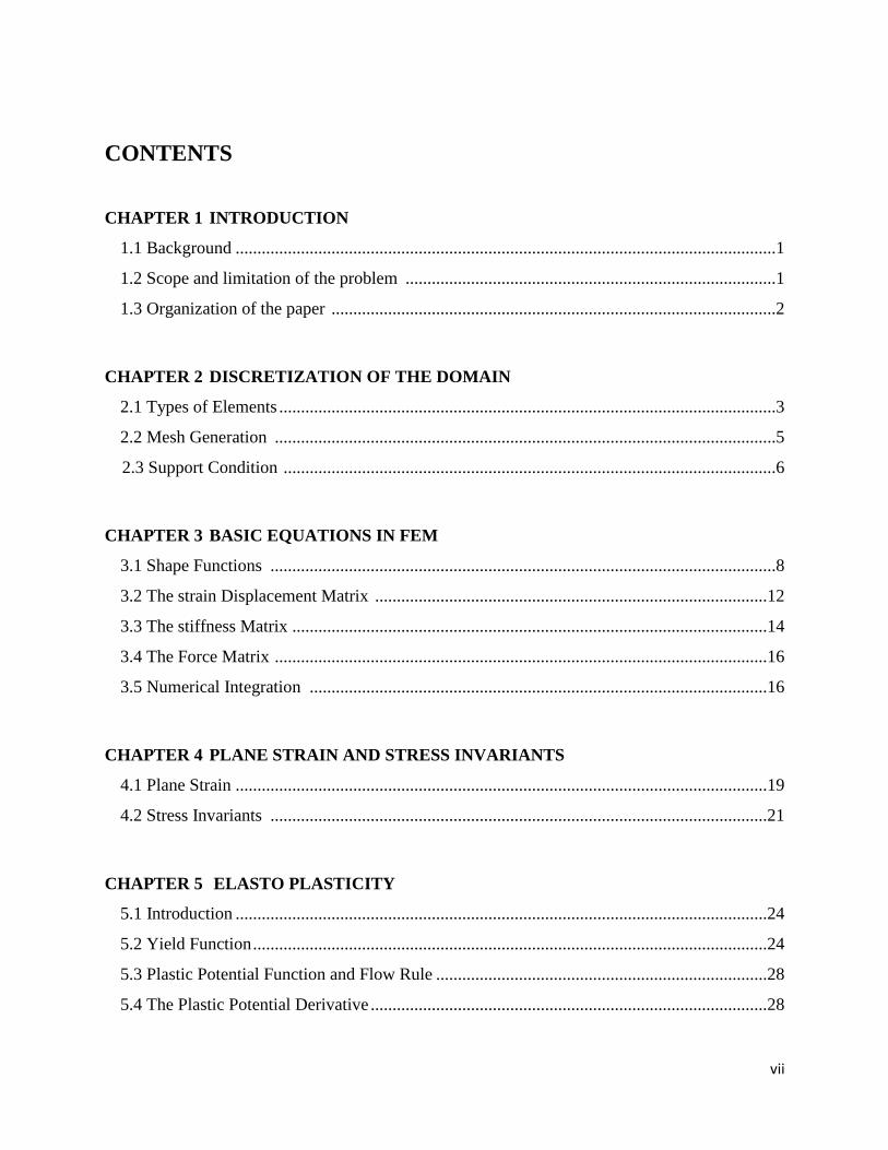
CONTENTS

CHAPTER 1 INTRODUCTION

1.1 Background ............................................................................................................................1

1.2 Scope and limitation of the problem .....................................................................................1

1.3 Organization of the paper ......................................................................................................2

CHAPTER 2 DISCRETIZATION OF THE DOMAIN

2.1 Types of Elements ..................................................................................................................3

2.2 Mesh Generation ...................................................................................................................5

2.3 Support Condition .................................................................................................................6

CHAPTER 3 BASIC EQUATIONS IN FEM

3.1 Shape Functions ....................................................................................................................8

3.2 The strain Displacement Matrix ..........................................................................................12

3.3 The stiffness Matrix .............................................................................................................14

3.4 The Force Matrix .................................................................................................................16

3.5 Numerical Integration .........................................................................................................16

CHAPTER 4 PLANE STRAIN AND STRESS INVARIANTS

4.1 Plane Strain ..........................................................................................................................19

4.2 Stress Invariants ..................................................................................................................21

CHAPTER 5 ELASTO PLASTICITY

5.1 Introduction ..........................................................................................................................24

5.2 Yield Function ......................................................................................................................24

5.3 Plastic Potential Function and Flow Rule ............................................................................28

5.4 The Plastic Potential Derivative ...........................................................................................28

viii

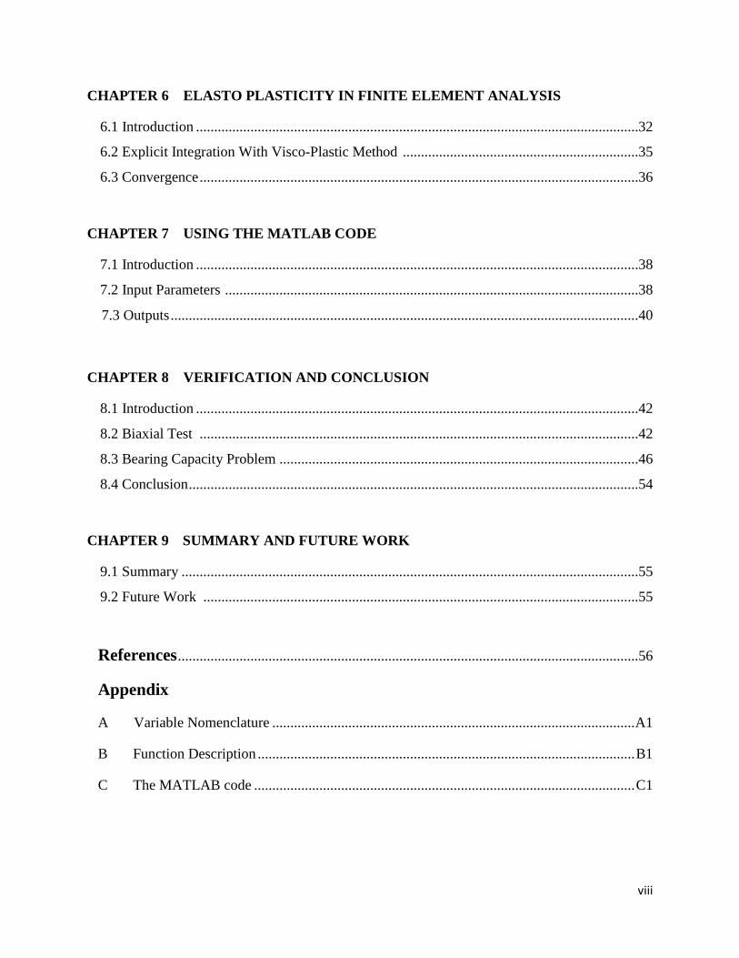
CHAPTER 6 ELASTO PLASTICITY IN FINITE ELEMENT ANALYSIS

6.1 Introduction ..........................................................................................................................32

6.2 Explicit Integration With Visco-Plastic Method .................................................................35

6.3 Convergence .........................................................................................................................36

CHAPTER 7 USING THE MATLAB CODE

7.1 Introduction ..........................................................................................................................38

7.2 Input Parameters ..................................................................................................................38

7.3 Outputs .................................................................................................................................40

CHAPTER 8 VERIFICATION AND CONCLUSION

8.1 Introduction ..........................................................................................................................42

8.2 Biaxial Test .........................................................................................................................42

8.3 Bearing Capacity Problem ...................................................................................................46

8.4 Conclusion ............................................................................................................................54

CHAPTER 9 SUMMARY AND FUTURE WORK

9.1 Summary ..............................................................................................................................55

9.2 Future Work ........................................................................................................................55

References ...............................................................................................................................56

Appendix

A Variable Nomenclature .................................................................................................... A1

B Function Description ........................................................................................................ B1

C The MATLAB code ......................................................................................................... C1

ix

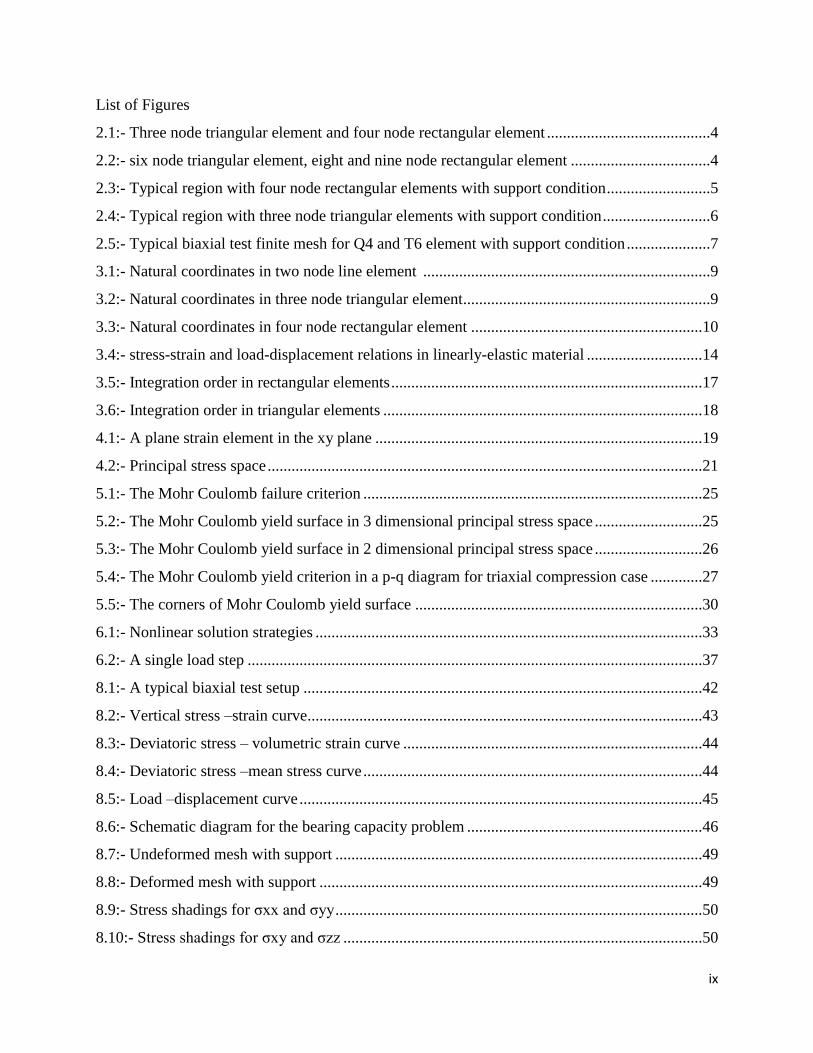
List of Figures

2.1:- Three node triangular element and four node rectangular element .........................................4

2.2:- six node triangular element, eight and nine node rectangular element ...................................4

2.3:- Typical region with four node rectangular elements with support condition ..........................5

2.4:- Typical region with three node triangular elements with support condition ...........................6

2.5:- Typical biaxial test finite mesh for Q4 and T6 element with support condition .....................7

3.1:- Natural coordinates in two node line element ........................................................................9

3.2:- Natural coordinates in three node triangular element ..............................................................9

3.3:- Natural coordinates in four node rectangular element ..........................................................10

3.4:- stress-strain and load-displacement relations in linearly-elastic material .............................14

3.5:- Integration order in rectangular elements ..............................................................................17

3.6:- Integration order in triangular elements ................................................................................18

4.1:- A plane strain element in the xy plane ..................................................................................19

4.2:- Principal stress space .............................................................................................................21

5.1:- The Mohr Coulomb failure criterion .....................................................................................25

5.2:- The Mohr Coulomb yield surface in 3 dimensional principal stress space ...........................25

5.3:- The Mohr Coulomb yield surface in 2 dimensional principal stress space ...........................26

5.4:- The Mohr Coulomb yield criterion in a p-q diagram for triaxial compression case .............27

5.5:- The corners of Mohr Coulomb yield surface ........................................................................30

6.1:- Nonlinear solution strategies .................................................................................................33

6.2:- A single load step ..................................................................................................................37

8.1:- A typical biaxial test setup ....................................................................................................42

8.2:- Vertical stress –strain curve...................................................................................................43

8.3:- Deviatoric stress – volumetric strain curve ...........................................................................44

8.4:- Deviatoric stress –mean stress curve .....................................................................................44

8.5:- Load –displacement curve .....................................................................................................45

8.6:- Schematic diagram for the bearing capacity problem ...........................................................46

8.7:- Undeformed mesh with support ............................................................................................49

8.8:- Deformed mesh with support ................................................................................................49

8.9:- Stress shadings for σxx and σyy ............................................................................................50

8.10:- Stress shadings for σxy and σzz ..........................................................................................50

x

8.11:- Displacement shadings ........................................................................................................51

8.12:- Deviatoric stress –mean stress curve ...................................................................................51

8.13:- Deviatoric stress –volumetric strain curve ..........................................................................52

8.14:- Vertical stress –vertical strain curve ...................................................................................52

8.15:- ‘Load’ –displacement curve ................................................................................................53

xi

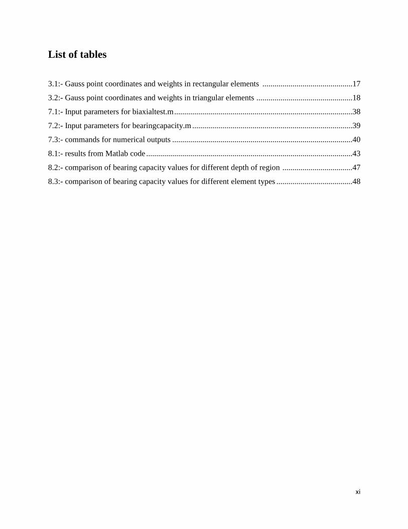
List of tables

3.1:- Gauss point coordinates and weights in rectangular elements .............................................17

3.2:- Gauss point coordinates and weights in triangular elements ................................................18

7.1:- Input parameters for biaxialtest.m .........................................................................................38

7.2:- Input parameters for bearingcapacity.m ................................................................................39

7.3:- commands for numerical outputs ..........................................................................................40

8.1:- results from Matlab code .......................................................................................................43

8.2:- comparison of bearing capacity values for different depth of region ...................................47

8.3:- comparison of bearing capacity values for different element types ......................................48

MATLAB FEM Code – From Elasticity to Plasticity

Feysel Nesru Sherif 1

CHAPTER 1

INTRODUCTION

1.1 Background

The finite element method is nowadays the most frequently used computational method in

engineering problems. In this numerical technique all complexities of a problem such as shape,

boundary and loading conditions are kept the same but the results obtained are approximate.

When using this method, calculations are robust due to the large number of unknowns leading to

a large pile of simultaneous equations for the user to solve. Hence the use of computer programs

to take care of these equations is one face of the method.

The evaluation of these simultaneous equations is done by using one of the matrix methods of

solving simultaneous equations. The MATLAB programming language is useful in illustrating

how to program the Finite element method due to the fact that it allows one to very quickly code

Numerical methods and has a vast predefined mathematical library suitable for handling

matrices.

1.2 Scope and limitation of the problem

The MATLAB Finite Element code presented here analyzes the stresses, strains and

displacements and gives the bearing capacity of a uniformly loaded strip footing on an Elasto-

plastic soil material in plane strain condition. Additionally a code for biaxial test is also included.

Bearing capacity analysis begins with the selection of the dimensions of the region which is

usually a rectangular region that is restrained vertically at the left and right sides and totally

restrained at the bottom end. When dividing the region in to smaller pieces five element types are

provided, three quadrilaterals (with 9,8 or 4 nodes) and two triangular (with 3 or 6 nodes).

There are two Load types to be considered; the first one is an external uniform load applied at the

top of the region, which the user needs to provide its length of distribution and magnitude. The

second type is the self weight of the soil which is generated by inserting the unit weight of the

soil material. When analysis begins all the functions developed work in the background to

provide the outputs for the user to see.

.



1.3 Organization of the paper

Any finite element analysis has the following main steps

Define a set of elements connected at nodes (discretization of the domain).

Assemble the global system, [K]{u} = {f}

Modify the global system by imposing essential (displacements) boundary conditions.

Solve the global system and obtain the global displacements, {u}

For each element, evaluate the strains and stresses at the nodes.

Chapter 2 covers about the types of elements and how the discretization is done and which

boundary conditions to be applied. In chapter 3 the basic equations of finite element analysis in

plane strain elements are presented in matrix form. Chapter 4 discusses about plane strain and

stress invariants. In chapter 5 the main features of an Elasto-plastic Mohr Coulomb material is

presented. The explicit integration scheme in load stepping for an Elasto-plastic material is

shown in chapter 6. In chapter 7 the main features of the code and how the user can implement it

is presented. Finally in chapter 8 the code is tested for validity with a biaxial test and a bearing

capacity problem and the results are compared with results from the PLAXIS software and with

theoretically solutions. Additionally the effect of element number and element type on these

results is discussed. Finally summary and future work based on this code are outlined. For quick

reference, all the functions and script files in the code are provided as an appendix. Additionally

a code for linear elastic materials from a previous work is attached as a reference in the

appendix.



CHAPTER 2

DISCRETIZATION OF THE DOMAIN

2.1 Types of Elements

The first step in the finite element analysis involves the division of the body into smaller Pieces,

known as finite elements. This is equivalent to replacing the body with an infinite number of

degrees of freedom by a system having finite number of degrees of freedom.

The shapes, number, and configurations of the elements are chosen in a way that the resulting

body resembles as closely as possible to that of the original body. The choice of the type of

element is dictated by the geometry of the body and the number of independent coordinates

necessary to describe the system. In plain strain analysis the geometry, material properties, and

the field variable of the system can be described in terms of two spatial coordinates i.e. x and y.

Elements are considered to be interconnected at specific points called nodes.

Nodes are the selected finite points at which basic unknowns are to be determined in the finite

element analysis .There are two types of nodes, external nodes and internal nodes. External

nodes are those which occur on the edges or surface of the elements and they may be common to

two or more elements. These nodes may be further classified as Primary nodes and Secondary

nodes. Primary nodes occur at the corners of elements. Secondary nodes occur along the side of

an element but not at corners. Internal nodes are the one which occur inside an element and they

are unique to each element. Based on this elements are categorized in to two groups.

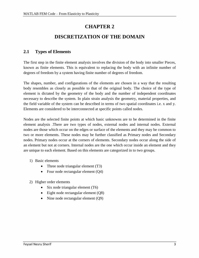
1) Basic elements

Three node triangular element (T3)

Four node rectangular element (Q4)

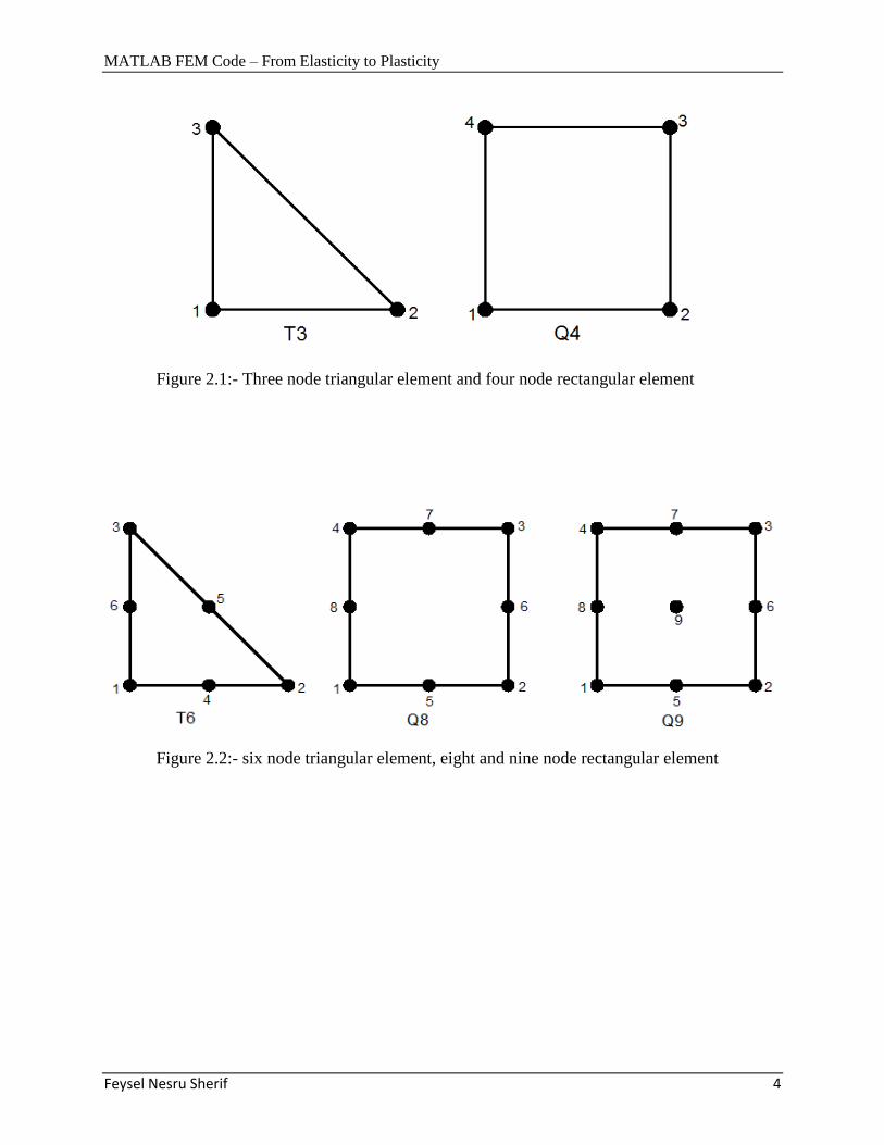
2) Higher order elements

Six node triangular element (T6)

Eight node rectangular element (Q8)

Nine node rectangular element (Q9)



Figure 2.1:- Three node triangular element and four node rectangular element

Figure 2.2:- six node triangular element, eight and nine node rectangular element



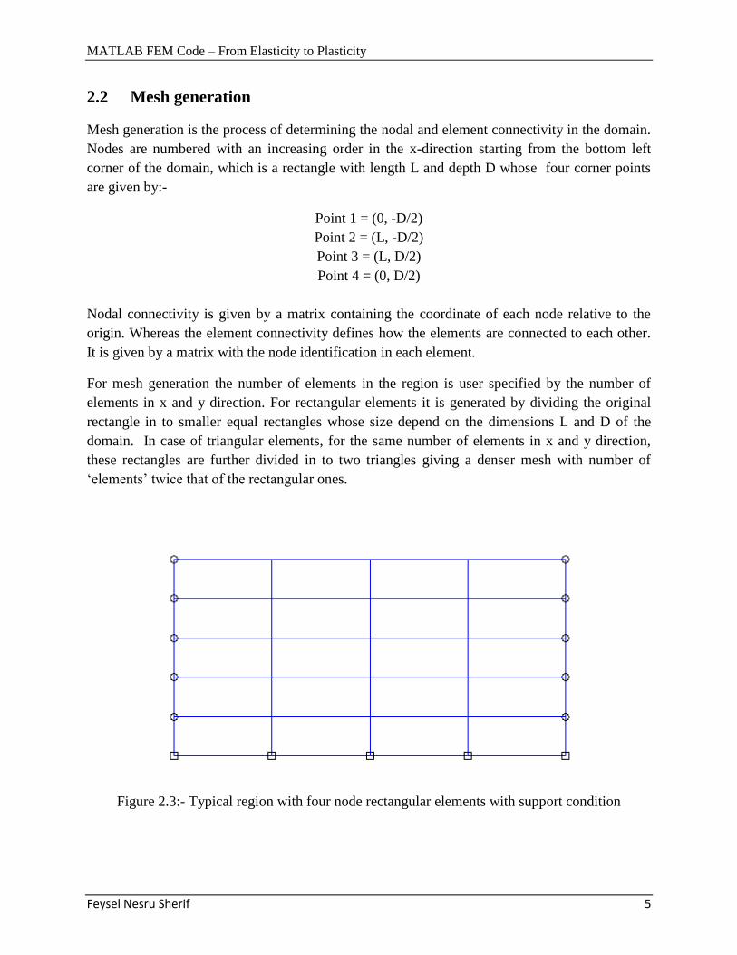
2.2 Mesh generation

Mesh generation is the process of determining the nodal and element connectivity in the domain.

Nodes are numbered with an increasing order in the x-direction starting from the bottom left

corner of the domain, which is a rectangle with length L and depth D whose four corner points

are given by:-

Point 1 = (0, -D/2)

Point 2 = (L, -D/2)

Point 3 = (L, D/2)

Point 4 = (0, D/2)

Nodal connectivity is given by a matrix containing the coordinate of each node relative to the

origin. Whereas the element connectivity defines how the elements are connected to each other.

It is given by a matrix with the node identification in each element.

For mesh generation the number of elements in the region is user specified by the number of

elements in x and y direction. For rectangular elements it is generated by dividing the original

rectangle in to smaller equal rectangles whose size depend on the dimensions L and D of the

domain. In case of triangular elements, for the same number of elements in x and y direction,

these rectangles are further divided in to two triangles giving a denser mesh with number of

„elements‟ twice that of the rectangular ones.

Figure 2.3:- Typical region with four node rectangular elements with support condition



Figure 2.4:- Typical region with three node triangular elements with support condition

2.3 Support condition

The restrained degrees of freedom in the system are two types

Translation in x and y direction for the nodes at the bottom of the domain which are

represented by black squares in the mesh and

Translation in x direction for the nodes at the left and right edge of the domain,

represented by black circles in the mesh.

These prescribed degrees of freedom, being zero, usually reduce the size of the stiffness matrix

and hence the calculation effort. Representation of support conditions in the finite element mesh

is shown in figures 2.3 and 2.4 above.



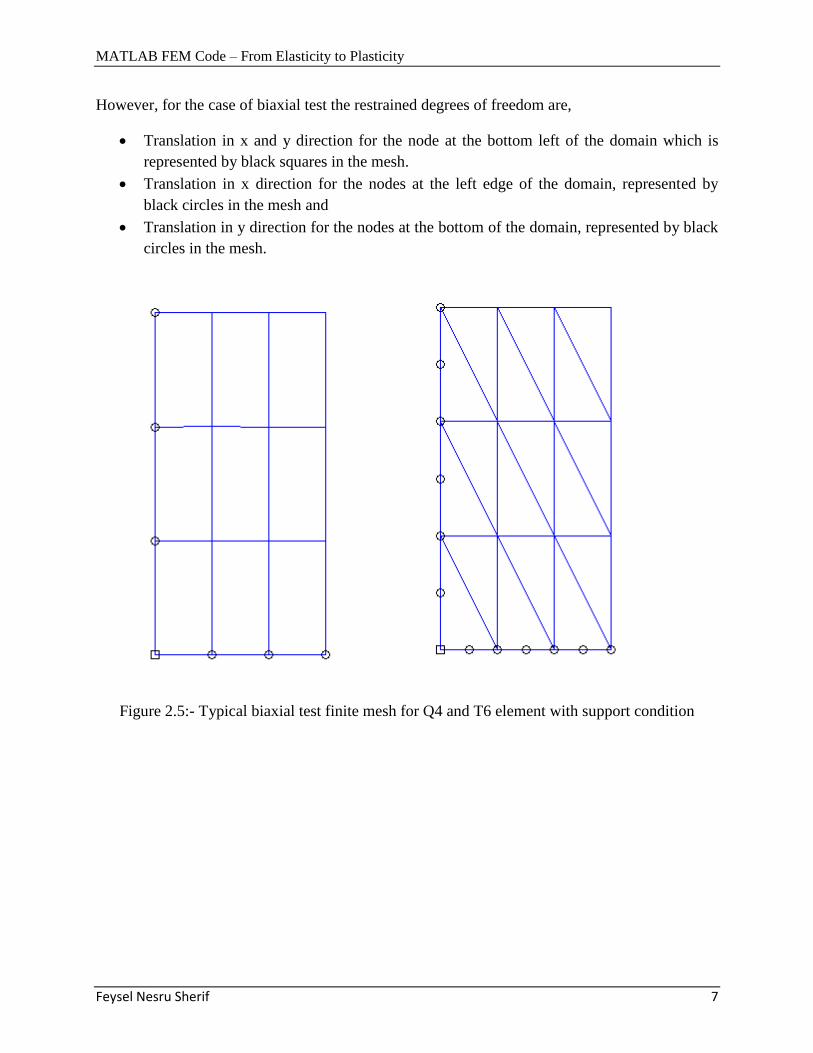
However, for the case of biaxial test the restrained degrees of freedom are,

Translation in x and y direction for the node at the bottom left of the domain which is

represented by black squares in the mesh.

Translation in x direction for the nodes at the left edge of the domain, represented by

black circles in the mesh and

Translation in y direction for the nodes at the bottom of the domain, represented by black

circles in the mesh.

Figure 2.5:- Typical biaxial test finite mesh for Q4 and T6 element with support condition



CHAPTER 3

BASIC EQUATIONS IN FEM

3.1 Shape functions

In the finite element analysis the aim is to find the field variables at nodal points by rigorous

analysis, assuming that at any point inside the element basic variable is a function of values at

nodal points of the element. This function which relates the field variable at any point within the

element to the field variables of nodal points is called shape function or interpolation function.

Taking displacement as the field variable this relationship can be expressed as:-

n

i i

i=1

u = N u ……………………….….……………....3.1

n

i i

i=1

v = N v ……………………………….………....3.2

Where

u= horizontal displacement

v= vertical displacement

ui = horizontal displacement at node i

vi = vertical displacement at node i

Ni = shape function expression at node i

Summation is over the number of nodes (n) of the element.

The shape functions are always expressed in terms of the natural coordinate system. A natural

coordinate system is a coordinate system which permits the specification of a point within the

element by a set of dimensionless numbers, whose magnitude never exceeds unity. It is obtained

by assigning weights to the nodal coordinates in defining the coordinate of any point inside the

element. Hence such system has the property that ith

coordinate has unit value at node i of the

element and zero value at all other nodes. As an illustration the use of shape functions is shown

for three element categories.



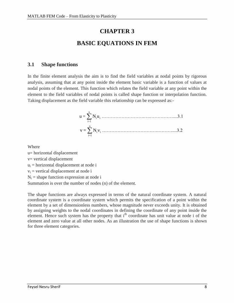
For a two node line element

Figure 3.1:- Natural coordinates in two node line element

From equation 3.1,

n

i i 1 1 2 2

i=1

u = N u = N u +N u

Where, 1

(1 )N

2

, 2

(1 )N

2

1

1 2

2

u = u

N Nu

……………………………………………....3.3

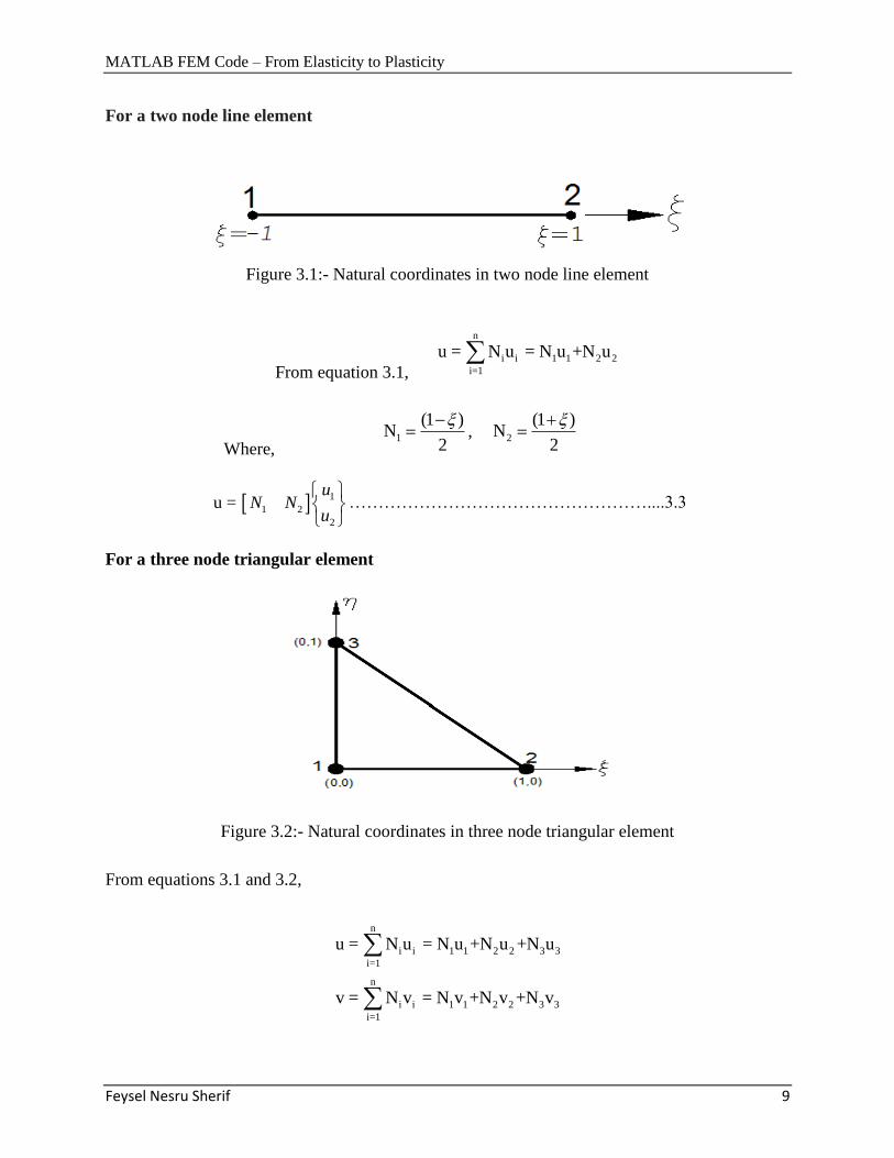
For a three node triangular element

Figure 3.2:- Natural coordinates in three node triangular element

From equations 3.1 and 3.2,

n

i i 1 1 2 2 3 3

i=1

u = N u = N u +N u +N u

n

i i 1 1 2 2 3 3

i=1

v = N v = N v +N v +N v



1N 1 , 2N and

3N

1

1

1 2 3 2

1 2 3 2

3

3

N 0 N 0 N 0u

0 N 0 N 0 Nv

u

v

u

v

u

v

…………………………....3.4

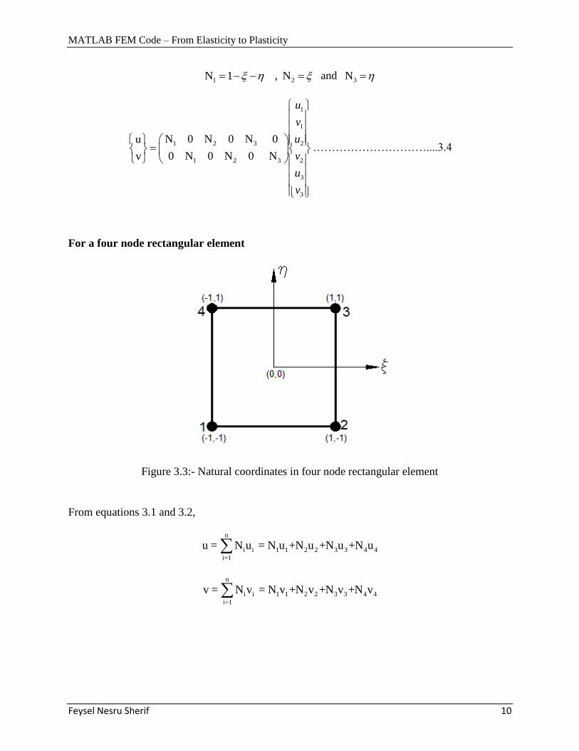
For a four node rectangular element

Figure 3.3:- Natural coordinates in four node rectangular element

From equations 3.1 and 3.2,

n

i i 1 1 2 2 3 3 4 4

i=1

u = N u = N u +N u +N u +N u

n

i i 1 1 2 2 3 3 4 4

i=1

v = N v = N v +N v +N v +N v



Where,

1

(1 )(1 )N

4

, 2

(1 )(1 )N

4

3

(1 )(1 )N

4

, 4

(1 )(1 )N

4

1

1

1 2 3 4

1 2 3 4

4

4

0 0 0 0 .u

0 0 0 0 .v

u

v

N N N N

N N N N

u

v

………….……....3.5

Using similar procedure, the shape functions for higher order elements can be formulated as

presented in the function shape_func in appendix C.



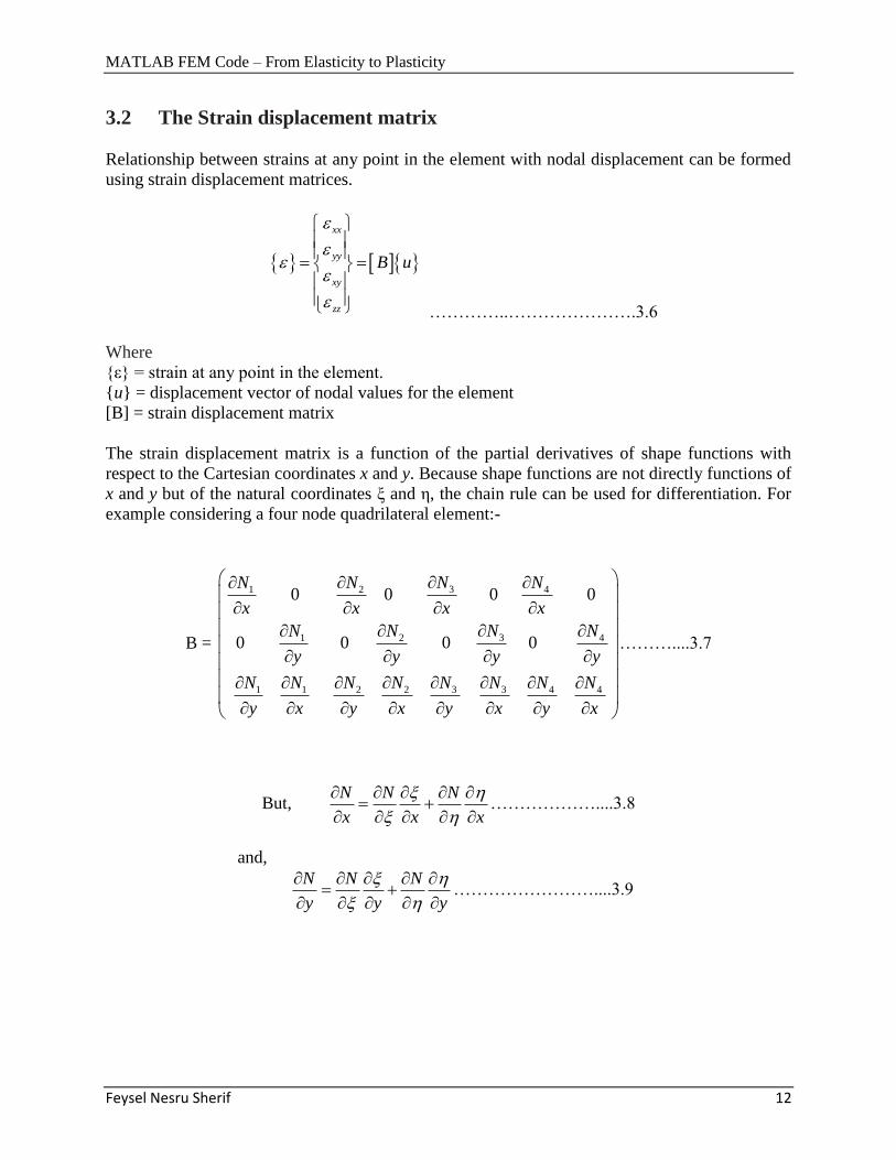
3.2 The Strain displacement matrix

Relationship between strains at any point in the element with nodal displacement can be formed

using strain displacement matrices.

xx

yy

xy

zz

B u

…………..………………….3.6

Where

{ε} = strain at any point in the element.

{u} = displacement vector of nodal values for the element

[B] = strain displacement matrix

The strain displacement matrix is a function of the partial derivatives of shape functions with

respect to the Cartesian coordinates x and y. Because shape functions are not directly functions of

x and y but of the natural coordinates ξ and η, the chain rule can be used for differentiation. For

example considering a four node quadrilateral element:-

B =

31 2 4

31 2 4

3 31 1 2 2 4 4

0 0 0 0

0 0 0 0

NN N N

x x x x

NN N N

y y y y

N NN N N N N N

y x y x y x y x

………....3.7

But, N N N

x x x

………………....3.8

and,

N N N

y y y

……………………....3.9



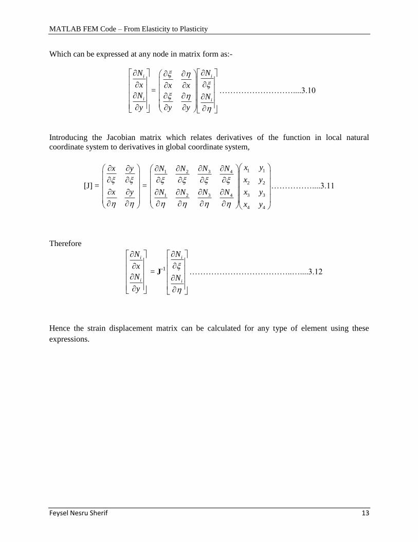
Which can be expressed at any node in matrix form as:-

i

i

N

x

N

y

=

i

i

N

x x

N

y y

………………………....3.10

Introducing the Jacobian matrix which relates derivatives of the function in local natural

coordinate system to derivatives in global coordinate system,

[J] =

x y

x y

=

1 131 2 4

2 2

3 331 2 4

4 4

x yNN N N

x y

x yNN N N

x y

……………....3.11

Therefore

i

i

N

x

N

y

= J-1

i

i

N

N

………………………………..…....3.12

Hence the strain displacement matrix can be calculated for any type of element using these

expressions.



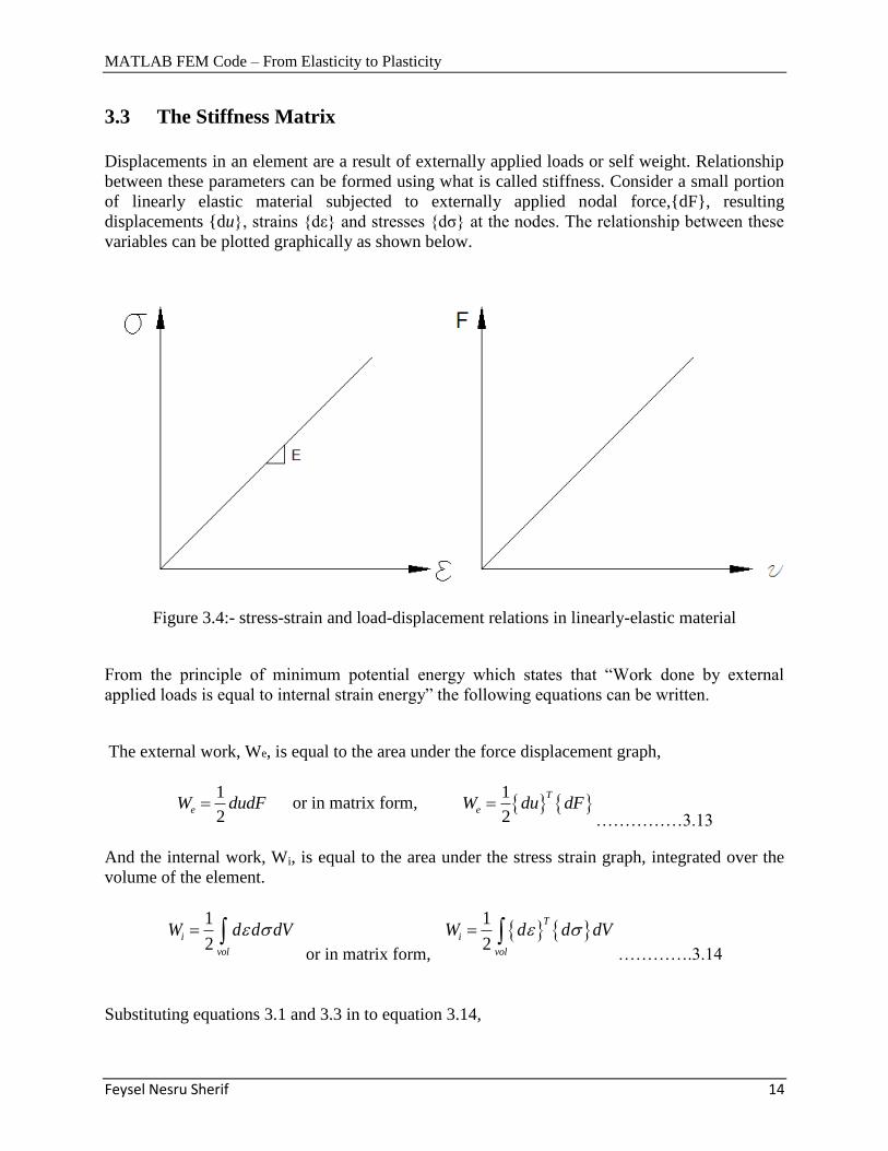
3.3 The Stiffness Matrix

Displacements in an element are a result of externally applied loads or self weight. Relationship

between these parameters can be formed using what is called stiffness. Consider a small portion

of linearly elastic material subjected to externally applied nodal force,{dF}, resulting

displacements {du}, strains {dε} and stresses {dσ} at the nodes. The relationship between these

variables can be plotted graphically as shown below.

Figure 3.4:- stress-strain and load-displacement relations in linearly-elastic material

From the principle of minimum potential energy which states that “Work done by external

applied loads is equal to internal strain energy” the following equations can be written.

The external work, We, is equal to the area under the force displacement graph,

1

2eW dudF or in matrix form,

1

2

T

eW du dF……………3.13

And the internal work, Wi, is equal to the area under the stress strain graph, integrated over the

volume of the element.

1

2i

vol

W d d dV or in matrix form,

1

2

T

i

vol

W d d dV ………….3.14

Substituting equations 3.1 and 3.3 in to equation 3.14,



1

[ ] [ ][ ]2

T T

i

vol

W du B C B du dV ……………………………….3.15

Equating the external and internal work and simplifying yields,

{ } [ ] [ ][ ] { }T

vol

dF B C B dV du ………………………….……….….3.16

The element stiffness matrix, [Ke], relating nodal forces {dF} to nodal displacements

{du}, is therefore:

[ ] [ ] [ ][ ]T

e

vol

K B C B dV …………………………..…………….3.17

Combining equations 3.16 and 3.17 gives the generalized equation of displacement based finite

element equation

{ } [ ]{ }F K u ………………………………………………..3.18

From which the nodal displacements are evaluated using

1{ } [ ]{ }u K F ……………………………………………………3.19

The stiffness matrix for the whole system which is called the global stiffness matrix (size= total

unknowns x total unknowns) can be assembled first by making all elements zero and then by

placing the stiffness matrix of each element in the “place” corresponding to the degree of

freedom of each point in the global system. The integral can be evaluated using the Gauss

numerical integration method.



3.4 The Force Matrix

Forces acting on an element can either be externally applied loads or due to the self weight. In

either case these loads can only be applied at the nodes as a point load, hence they have to be

distributed to the corresponding nodes using the shape functions using the expressions below.

{ } [ ] { } [ ] { }T T

b

vol

F N X dV N T dl ………………………....3.20

While,

0{ }bX

Where

ϒ = self weight of material {T} = externally applied uniform load

N = shape function

3.5 Numerical integration

During the evaluation of the stiffness matrix and the force or self weight matrix, integrations

over the volume or the area of the element are encountered .Numerical integration is essential for

practical evaluation of these integrals over the domain of the element. The common method of

integration is the Gauss integration method since it uses a minimal number of sample points to

achieve a desired level of accuracy.

Before integration, the number of integration points (integration order) must be selected. From

which the corresponding coordinates and weights of each point is selected and the integration is

performed using:-

1 1

1 11 1

( , ) ( , )n n

j i

j i

f d d W W f

…………………………….3.21

Where

𝜉= natural x coordinate of the Gauss sample point

η = natural y coordinate of the Gauss sample point

W= weight of the Gauss sample point

n=number of integration points (integration order)

f (ξ,η) =value of the function at the sample points



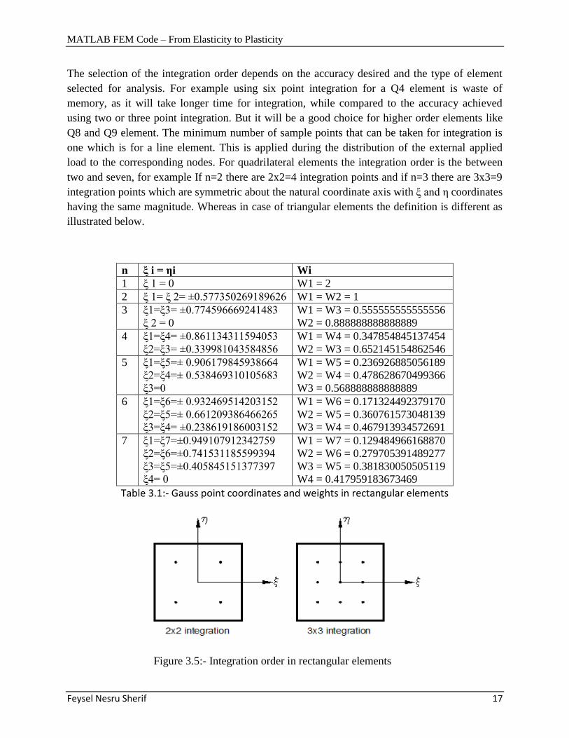
The selection of the integration order depends on the accuracy desired and the type of element

selected for analysis. For example using six point integration for a Q4 element is waste of

memory, as it will take longer time for integration, while compared to the accuracy achieved

using two or three point integration. But it will be a good choice for higher order elements like

Q8 and Q9 element. The minimum number of sample points that can be taken for integration is

one which is for a line element. This is applied during the distribution of the external applied

load to the corresponding nodes. For quadrilateral elements the integration order is the between

two and seven, for example If n=2 there are 2x2=4 integration points and if n=3 there are 3x3=9

integration points which are symmetric about the natural coordinate axis with ξ and η coordinates

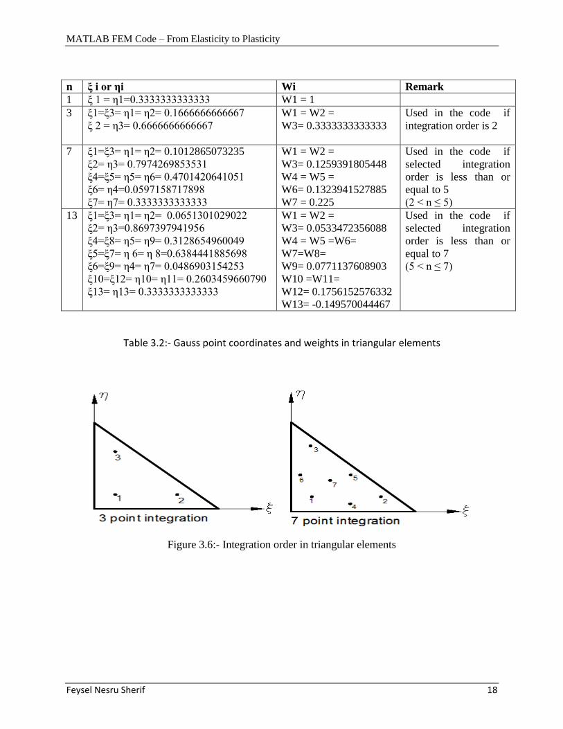
having the same magnitude. Whereas in case of triangular elements the definition is different as

illustrated below.

n ξ i = ηi Wi

1 ξ 1 = 0 W1 = 2

2 ξ 1= ξ 2= ±0.577350269189626 W1 = W2 = 1

3 ξ1=ξ3= ±0.774596669241483

ξ 2 = 0

W1 = W3 = 0.555555555555556

W2 = 0.888888888888889

4 ξ1=ξ4= ±0.861134311594053

ξ2=ξ3= ±0.339981043584856

W1 = W4 = 0.347854845137454

W2 = W3 = 0.652145154862546

5 ξ1=ξ5=± 0.906179845938664

ξ2=ξ4=± 0.538469310105683

ξ3=0

W1 = W5 = 0.236926885056189

W2 = W4 = 0.478628670499366

W3 = 0.568888888888889

6 ξ1=ξ6=± 0.932469514203152

ξ2=ξ5=± 0.661209386466265

ξ3=ξ4= ±0.238619186003152

W1 = W6 = 0.171324492379170

W2 = W5 = 0.360761573048139

W3 = W4 = 0.467913934572691

7 ξ1=ξ7=±0.949107912342759

ξ2=ξ6=±0.741531185599394

ξ3=ξ5=±0.405845151377397

ξ4= 0

W1 = W7 = 0.129484966168870

W2 = W6 = 0.279705391489277

W3 = W5 = 0.381830050505119

W4 = 0.417959183673469

Table 3.1:- Gauss point coordinates and weights in rectangular elements

Figure 3.5:- Integration order in rectangular elements



n ξ i or ηi Wi Remark

1 ξ 1 = η1=0.3333333333333 W1 = 1

3 ξ1=ξ3= η1= η2= 0.1666666666667

ξ 2 = η3= 0.6666666666667

W1 = W2 =

W3= 0.3333333333333

Used in the code if

integration order is 2

7 ξ1=ξ3= η1= η2= 0.1012865073235

ξ2= η3= 0.7974269853531

ξ4=ξ5= η5= η6= 0.4701420641051

ξ6= η4=0.0597158717898

ξ7= η7= 0.3333333333333

W1 = W2 =

W3= 0.1259391805448

W4 = W5 =

W6= 0.1323941527885

W7 = 0.225

Used in the code if

selected integration

order is less than or

equal to 5

(2 < n ≤ 5)

13 ξ1=ξ3= η1= η2= 0.0651301029022

ξ2= η3=0.8697397941956

ξ4=ξ8= η5= η9= 0.3128654960049

ξ5=ξ7= η 6= η 8=0.6384441885698

ξ6=ξ9= η4= η7= 0.0486903154253

ξ10=ξ12= η10= η11= 0.2603459660790

ξ13= η13= 0.3333333333333

W1 = W2 =

W3= 0.0533472356088

W4 = W5 =W6=

W7=W8=

W9= 0.0771137608903

W10 =W11=

W12= 0.1756152576332

W13= -0.149570044467

Used in the code if

selected integration

order is less than or

equal to 7

(5 < n ≤ 7)

Table 3.2:- Gauss point coordinates and weights in triangular elements

Figure 3.6:- Integration order in triangular elements



CHAPTER 4

PLANE STRAIN AND STRESS INVARIANTS

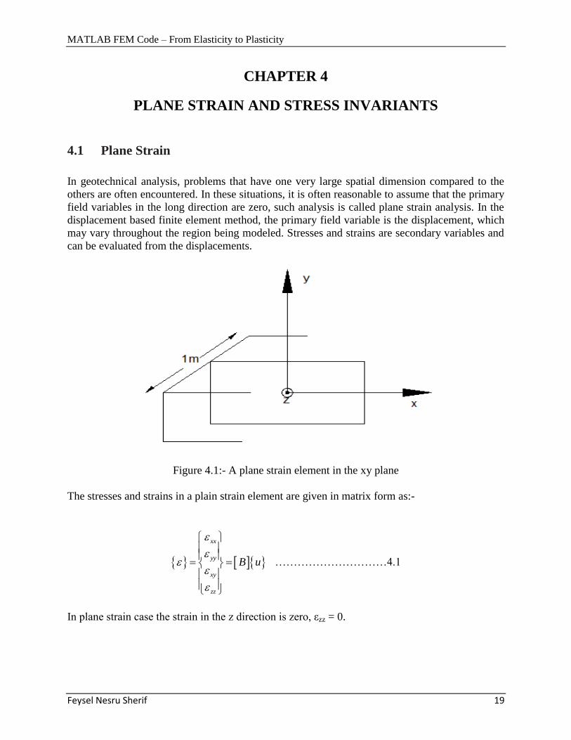
4.1 Plane Strain

In geotechnical analysis, problems that have one very large spatial dimension compared to the

others are often encountered. In these situations, it is often reasonable to assume that the primary

field variables in the long direction are zero, such analysis is called plane strain analysis. In the

displacement based finite element method, the primary field variable is the displacement, which

may vary throughout the region being modeled. Stresses and strains are secondary variables and

can be evaluated from the displacements.

Figure 4.1:- A plane strain element in the xy plane

The stresses and strains in a plain strain element are given in matrix form as:-

xx

yy

xy

zz

B u

…………………………4.1

In plane strain case the strain in the z direction is zero, εzz = 0.



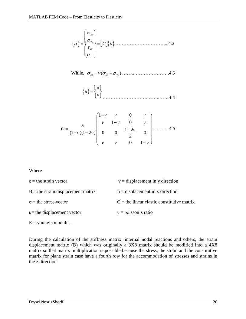
xx

yy

xy

zz

C

…………………………....4.2

While, ( )zz xx yy ……..………………….4.3

u

vu

……………………….……..……4.4

1 0

1 0

1 2(1 )(1 2 ) 0 0 0

2

0 1

EC

………..4.5

Where

ε = the strain vector v = displacement in y direction

B = the strain displacement matrix u = displacement in x direction

σ = the stress vector C = the linear elastic constitutive matrix

u= the displacement vector ν = poisson‟s ratio

E = young‟s modulus

During the calculation of the stiffness matrix, internal nodal reactions and others, the strain

displacement matrix (B) which was originally a 3X8 matrix should be modified into a 4X8

matrix so that matrix multiplication is possible because the stress, the strain and the constitutive

matrix for plane strain case have a fourth row for the accommodation of stresses and strains in

the z direction.



4.2 Stress Invariants

As shown above, a plane strain state of stress can be specified with four components with a fixed

coordinate system (σxx, σyy, τxy, σzz). The magnitude of these stresses depends on the orientation

of the chosen coordinate system. Another way of specifying stress state is using the principal

stresses (σ1, σ2, σ3), which act in the same direction and have the same magnitude for a given

stress state, regardless of the chosen orientation of coordinate axes. Principal stresses are

therefore frequently used to show a stress point in space. The plot of the principal stresses on a

three dimensional graph, known as principal stress space, shows the stress state and stress paths.

Figure 3.2 shows a principal stress space.

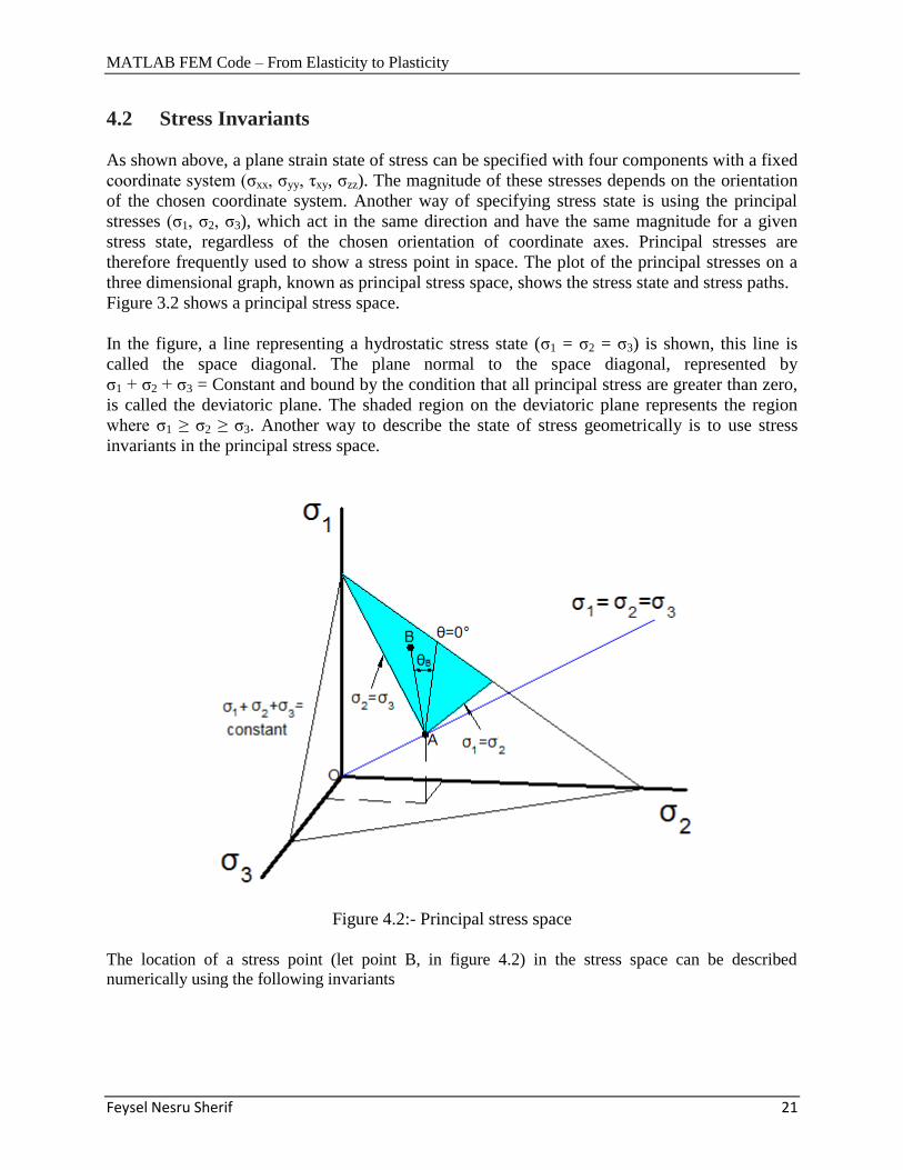
In the figure, a line representing a hydrostatic stress state (σ1 = σ2 = σ3) is shown, this line is

called the space diagonal. The plane normal to the space diagonal, represented by

σ1 + σ2 + σ3 = Constant and bound by the condition that all principal stress are greater than zero,

is called the deviatoric plane. The shaded region on the deviatoric plane represents the region

where σ1 ≥ σ2 ≥ σ3. Another way to describe the state of stress geometrically is to use stress

invariants in the principal stress space.

Figure 4.2:- Principal stress space

The location of a stress point (let point B, in figure 4.2) in the stress space can be described

numerically using the following invariants



1 2 3

3s

………………………..………………..…4.6

2 2 2

1 2 2 3 3 1

1( ) ( ) ( )

3t

………………4.7

1 2 3

1 3

2( )1tan 1

( )3

………………………..……4.8

The distance along the space diagonal from the origin to the deviatoric plane (OA) is represented

by the stress invariant s, while t is the distance from the space diagonal to the stress point (AB)

and Lode angle (ϴ) is the angular position of the stress point in the deviatoric plane. The value of

Lode‟s angle on the plane varies between the extremities of the intermediate principal stresses

as:-

ϴ=+30°, triaxial compression, |σ’1| ≥|σ’2| = |σ’3|and ϴ=-30°, triaxial extension, |σ’1| =|σ’2| ≥ |σ’3| In Geotechnical Engineering, the most widely used invariants are mean and deviatoric stress which

can be expressed in terms of Cartesian stresses as:-

3

xx yy zz

m p

……………………….…...……4.9

Rewriting equation 4.7 in Cartesian form,

2 2 2 21( ) ( ) ( ) 6

3xx yy yy zz zz xx xyt

………4.10

. From which, 3

2q t

……………………………………4.11



Similarly the Lode angle is given by

1 3

3

3 61sin

3

J

t

…………………………….……4.12

where 2

3 x y z z xyJ s s s s ……………………….4.13

x xxs p ……………………………..4.14

y yys p ………………….………….4.15

z zzs p ……………………….…….4.16

The principal stresses can be expressed in terms of these invariants as:-

1

2 2sin( )

3 3p q

……………………….………….4.17

2

2sin( )

3p q

………….…………….………….…….4.18

3

2 2sin( )

3 3p q

…………………………………..4.19

Note that, since compression is negative, in these equations the value of p is negative and that of

q is positive.



CHAPTER 5

ELASTO PLASTICITY

5.1 Introduction

Due to the complexity of real soil behavior, a single constitutive model that can describe all facts

of behavior, with a reasonable number of input parameters, has not been achieved. Consequently,

there are many soil models available, each of which has different advantages and disadvantages.

The Mohr-Coulomb material model is one of the well known elastic perfectly plastic soil

models. The main features of this model are discussed below.

5.2 Yield Function

Based on the current stress state, an Elasto-plastic material behaves either as an elastic solid or a

plastic solid. The transition from elasticity to plasticity is described by the yield criterion which

forms a surface in three dimensional principle stress space. Stress states lying within the yield

surface are regarded as elastic, while stress states lying on the yield surface are plastic. As the

material deforms plastically, the stresses must remain on the yield surface and so stress states

lying outside the yield surface are inadmissible and must be redistributed through an iterative

procedure. Algebraically, these surfaces are expressed in terms of yield or failure function (F).

This function, which has units of stress, is dependent on material properties and invariant

combinations of the stress components. The derivation of the Mohr Coulomb yield function is

discussed below.

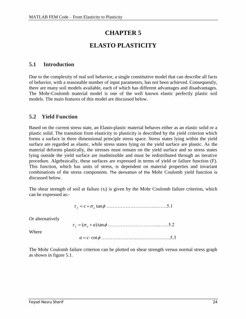
The shear strength of soil at failure (τf) is given by the Mohr Coulomb failure criterion, which

can be expressed as:-

tanf nc ………………………….…….5.1

Or alternatively

( ) tanf n a …………………………..……5.2

Where

cota c …………………………………….5.3

The Mohr Coulomb failure criterion can be plotted on shear strength versus normal stress graph

as shown in figure 5.1.



Figure 5.1:- The Mohr Coulomb failure criterion

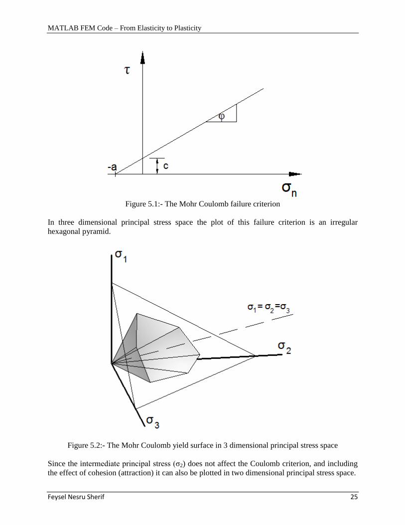
In three dimensional principal stress space the plot of this failure criterion is an irregular

hexagonal pyramid.

Figure 5.2:- The Mohr Coulomb yield surface in 3 dimensional principal stress space

Since the intermediate principal stress (σ2) does not affect the Coulomb criterion, and including

the effect of cohesion (attraction) it can also be plotted in two dimensional principal stress space.



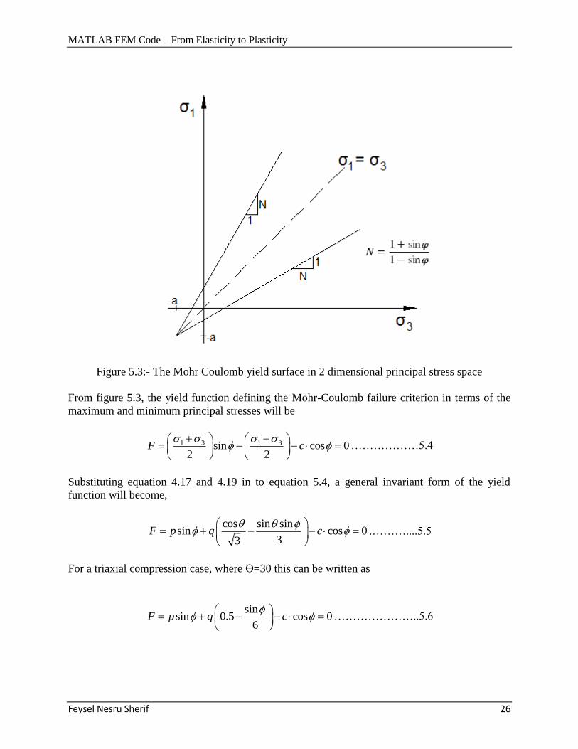
Figure 5.3:- The Mohr Coulomb yield surface in 2 dimensional principal stress space

From figure 5.3, the yield function defining the Mohr-Coulomb failure criterion in terms of the

maximum and minimum principal stresses will be

1 3 1 3sin cos 02 2

F c

………………5.4

Substituting equation 4.17 and 4.19 in to equation 5.4, a general invariant form of the yield

function will become,

cos sin sinsin cos 0

33F p q c

.………....5.5

For a triaxial compression case, where ϴ=30 this can be written as

sinsin 0.5 cos 0

6F p q c

…………………..5.6



Since, cos sinc a

With attraction (a = negative), Equation 5.6 can be rearranged as

6sin( )

3 sinq p a

………………………………………5.7

With, 6sin

3 sinM

………………..…………………5.8

Equation 5.7 simplifies to

( )q M p a …………………………………5.9

Equation 5.9 is the plot of the Mohr-Coulomb failure criterion in a triaxial stress space

commonly known as, p-q diagram.

Figure 5.4:- The Mohr Coulomb yield criterion in a p-q diagram for triaxial compression case



5.3 Plastic potential Function and Flow rule

The plastic potential function, G, specifies the direction of the plastic strain increment, which is proportional to the derivative of G with respect to the corresponding stress.

{ }p G

………………………………………5.10

Where Δλ is a scalar quantity called plastic multiplier. This scalar is not a property of the

material but rather a property of the flow conditions. The plastic potential function is defined by

cos sin sinsin cos 0

33G p q c

.…..……5.11.

When the friction angle (υ) and dilatancy angle (ψ) are equal, the flow condition is said to be

associated flow and the yield and plastic potential function are identical and equation 5.10 can be

written as

{ }p F

……………………….5.12

Otherwise the flow is said to be non-associated flow.

5.4 The Plastic potential Derivative

During the calculation of plastic strain increments, the plastic potential derivative should be

evaluated according to chain rule.

G G p G q G

p q

…………….5.13

Expressing the quantities q and ϴ in terms of J2 and J3 simplifies the derivative process,

32

2 3

JJG G p G G

p J J

….……….5.14

Where

2

23

qJ and 3 0.385sin(3 )J



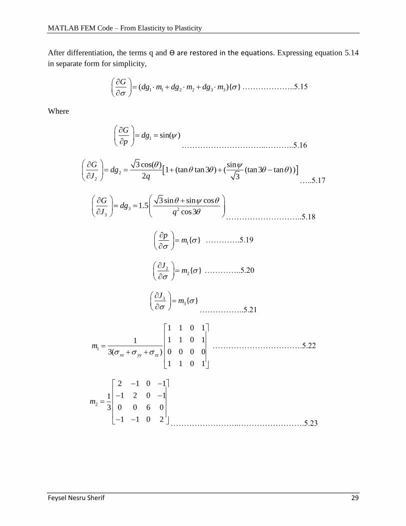
After differentiation, the terms q and ϴ are restored in the equations. Expressing equation 5.14

in separate form for simplicity,

1 1 2 2 3 3( ){ }

Gdg m dg m dg m

………………..5.15

Where

1 sin( )

Gdg

p

…………………………..………..5.16

2

2

3 cos( ) sin1 (tan tan3 ) ( (tan 3 tan ) )

2 3

Gdg

J q

…..5.17

3 2

3

3 sin sin cos1.5

cos3

Gdg

J q

………………………..5.18

1{ }p

m

………….5.19

22{ }

Jm

…………..5.20

33{ }

Jm

……………..5.21

1

1 1 0 1

1 1 0 11

0 0 0 03( )

1 1 0 1

xx yy zz

m

…………………………….5.22

2

2 1 0 1

1 2 0 11

0 0 6 03

1 1 0 2

m

……………………..…………………….5.23



3

1

3 23

2

x z xy z

z y xy x

xy xy z xy

z x xy z

s s s

s s sm

s

s s s

…………………………………….5.24

xx

yy

xy

zz

………………………………………….5.25

x xxs p ……………5.26

y yys p ……………5.27

z zzs p ……………5.28

The yield and plastic potential functions of a Mohr Coulomb material are a function of the Lode

angle, which in turn is variable depending on the stress state, as shown in equations 5.5 and

5.11.During the calculation of the plastic strains the plastic potential derivative becomes

indeterminate when the lode angle approaches the corners of the hexagonal surface (±30°).

Figure 5.5:- The corners of Mohr Coulomb yield surface



This problem can be resolved by smoothening the corners of the yield surface if the lode angle

gets close enough to ±30°. This is achieved by substituting ϴ=±30° in equation 5.11 depending

on whether it is getting close to triaxial compression or extension. In these cases the terms dg2

and dg3 in equations 5.17 and 5.18 respectively should be modified as,

For ϴ≈30° triaxial compression case

2

0.25(3 sin )dg

q …………………5.29

3 0dg ……………….……5.30

For ϴ≈-30° triaxial extension case

2

0.25(3 sin )dg

q

……………………5.31

3 0dg ……………..………5.32



CHAPTER 6

ELASTO PLASTICITY IN FINITE ELEMENT ANALYSIS

6.1 Introduction

Non-linear problems in finite element analysis can be grouped into the following three

categories, based on the sources of non-linearity:

1. Material Nonlinearity Problems

2. Geometric Nonlinearity Problems and

3. Both material and Geometric Nonlinearity Problems.

Here, only the case of Material Nonlinearity is discussed. Nonlinearity due to an Elasto Plastic

material causes the governing finite element equations to be reduced to the following

incremental form,

[ ]{ } { }i iK u f ……………………….………6.1

Where

[ K] = the global system stiffness matrix

{Δu} = the vector of incremental nodal displacements

{Δf} = the vector of incremental nodal forces and

i = the increment number

To obtain a solution to a boundary value problem, the change in boundary conditions is applied

in a series of increments and for each increment equation 6.1 must be solved. The final solution

is obtained by summing the results of each increment. Due to the nonlinear constitutive behavior

of the Mohr Coulomb material, the global stiffness matrix is dependent on the current stress and

strain levels and therefore is not constant, but varies over an increment.

In practical Finite Element Analysis, two main types of solution strategies can be used to solve

this equation. The first method, known as the Tangent Stiffness Method, considers the reduction

of the material stiffness as failure is approached. Hence the global stiffness matrix is updated at

each iteration to achieve convergence. In this method the numbers of iterations needed to achieve

convergence are relatively small but the cost of computer memory, due to the formation of the

global stiffness matrix at each iteration, is very large and hence is not used here.



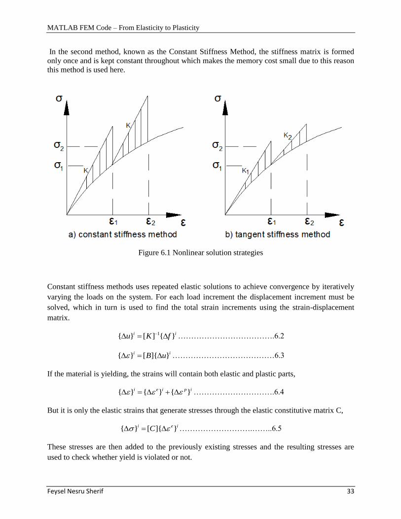
In the second method, known as the Constant Stiffness Method, the stiffness matrix is formed

only once and is kept constant throughout which makes the memory cost small due to this reason

this method is used here.

Figure 6.1 Nonlinear solution strategies

Constant stiffness methods uses repeated elastic solutions to achieve convergence by iteratively

varying the loads on the system. For each load increment the displacement increment must be

solved, which in turn is used to find the total strain increments using the strain-displacement

matrix.

1{ } [ ] { }i iu K f ……………………………….6.2

{ } [ ]{ }i iB u …………………………………6.3

If the material is yielding, the strains will contain both elastic and plastic parts,

{ } { } { }i e i p i ………………………….6.4

But it is only the elastic strains that generate stresses through the elastic constitutive matrix C,

{ } [ ]{ }i e iC ……………………….……..6.5

These stresses are then added to the previously existing stresses and the resulting stresses are

used to check whether yield is violated or not.



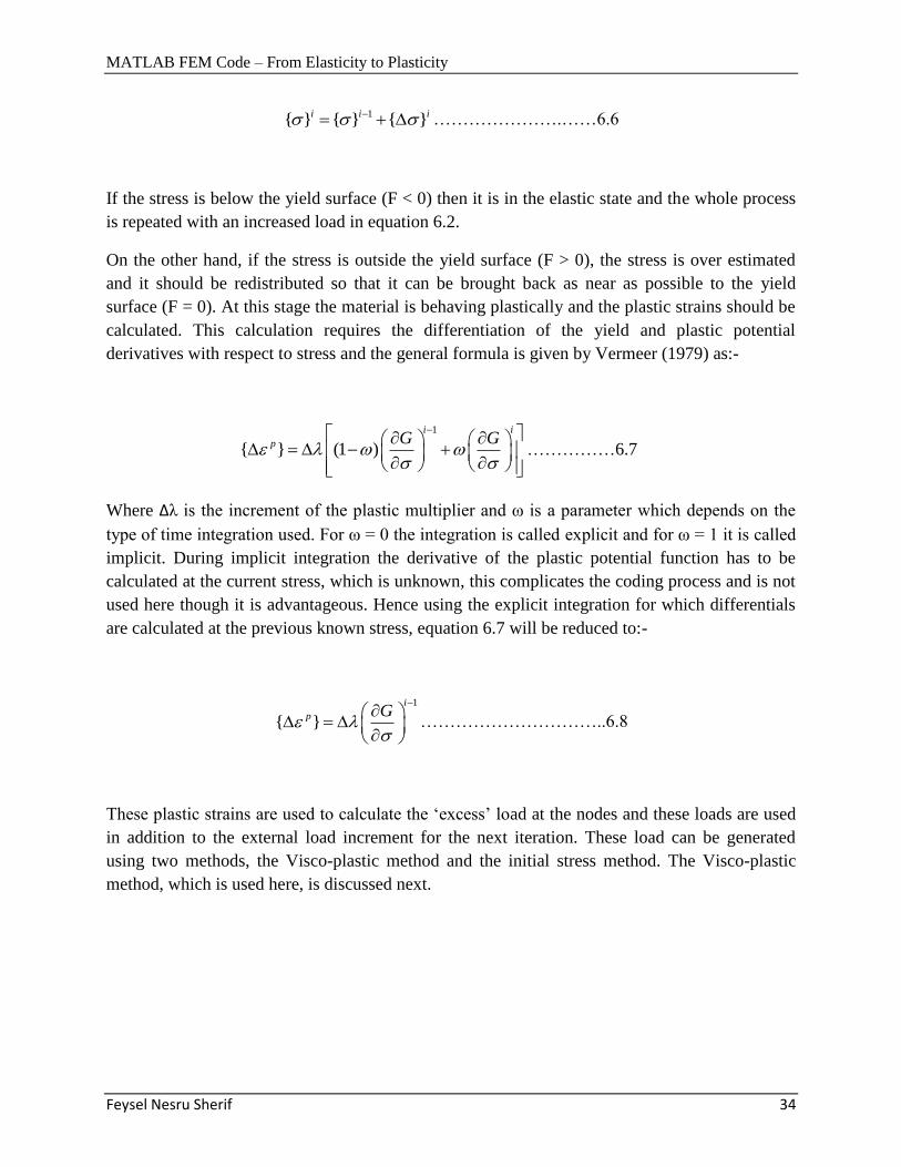
1{ } { } { }i i i ………………….……6.6

If the stress is below the yield surface (F < 0) then it is in the elastic state and the whole process

is repeated with an increased load in equation 6.2.

On the other hand, if the stress is outside the yield surface (F > 0), the stress is over estimated

and it should be redistributed so that it can be brought back as near as possible to the yield

surface (F = 0). At this stage the material is behaving plastically and the plastic strains should be

calculated. This calculation requires the differentiation of the yield and plastic potential

derivatives with respect to stress and the general formula is given by Vermeer (1979) as:-

1

{ } (1 )

i i

p G G

……………6.7

Where Δλ is the increment of the plastic multiplier and ω is a parameter which depends on the

type of time integration used. For ω = 0 the integration is called explicit and for ω = 1 it is called

implicit. During implicit integration the derivative of the plastic potential function has to be

calculated at the current stress, which is unknown, this complicates the coding process and is not

used here though it is advantageous. Hence using the explicit integration for which differentials

are calculated at the previous known stress, equation 6.7 will be reduced to:-

1

{ }

i

p G

…………………………..6.8

These plastic strains are used to calculate the „excess‟ load at the nodes and these loads are used

in addition to the external load increment for the next iteration. These load can be generated

using two methods, the Visco-plastic method and the initial stress method. The Visco-plastic

method, which is used here, is discussed next.



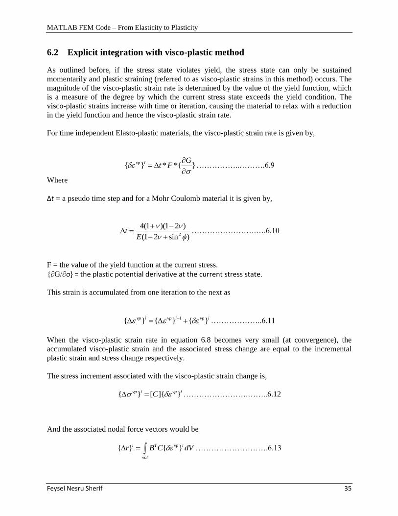
6.2 Explicit integration with visco-plastic method

As outlined before, if the stress state violates yield, the stress state can only be sustained

momentarily and plastic straining (referred to as visco-plastic strains in this method) occurs. The

magnitude of the visco-plastic strain rate is determined by the value of the yield function, which

is a measure of the degree by which the current stress state exceeds the yield condition. The

visco-plastic strains increase with time or iteration, causing the material to relax with a reduction

in the yield function and hence the visco-plastic strain rate.

For time independent Elasto-plastic materials, the visco-plastic strain rate is given by,

{ } * *{ }vp i Gt F

……………..……….6.9

Where

Δt = a pseudo time step and for a Mohr Coulomb material it is given by,

2

4(1 )(1 2 )

(1 2 sin )t

E

…………………….….6.10

F = the value of the yield function at the current stress.

{∂G/∂σ} = the plastic potential derivative at the current stress state.

This strain is accumulated from one iteration to the next as

1{ } { } { }vp i vp i vp i ………………..6.11

When the visco-plastic strain rate in equation 6.8 becomes very small (at convergence), the

accumulated visco-plastic strain and the associated stress change are equal to the incremental

plastic strain and stress change respectively.

The stress increment associated with the visco-plastic strain change is,

{ } [ ]{ }vp i vp iC …………………….……..6.12

And the associated nodal force vectors would be

{ } { }i T vp i

vol

r B C dV ……………………….6.13



These nodal reactions are accumulated at each iteration by summing equation 6.13 for all

elements with yielding gauss points. Finally the applied load vector would take the form,

1{ } { } { }i i T vp i

all volelements

f f B C dV …………..6.14

This load is then used in equation 6.2 and the process is repeated until convergence is achieved.

If convergence is achieved, the stresses, strains and displacements from the last iteration are

recorded for use in the next load step.

6.3 Convergence

During the iteration process from equation 6.2 through 6.14 the process is repeated until the

stresses are close enough to the yield surface within a certain error which should be less than a

predefined tolerance which is set to be 0.01. When this criterion is met the solution is said to be

converged. Convergence is indicated by either of the following

The incremental displacements from equation 6.2 is nearly the same from one iteration to

the next

The yield function, F is too small

The visco-plastic strain is too small

The stress increment from equation 6.5 is nearly the same from one iteration to the next

To calculate the error the displacement condition is used. In this condition the difference

between the absolute maximum of the incremental displacements in iteration i and iteration i-1

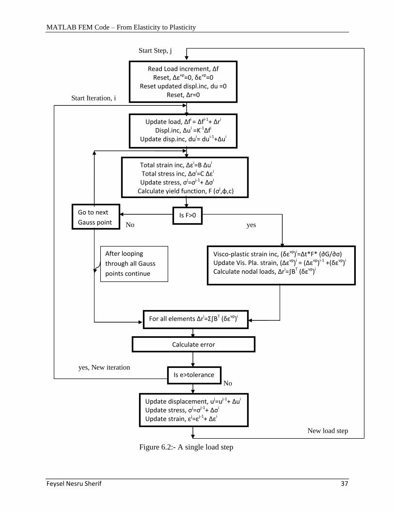
should be less than the predefined tolerance. The whole load stepping in shown in the flow chart

in the next page.



Start Step, j

Start Iteration, i

No yes

yes, New iteration

No

New load step

Figure 6.2:- A single load step

Is e>tolerance

Total strain inc, Δεi=B Δui Total stress inc, Δσi=C Δεi Update stress, σj=σj-1+ Δσi

Calculate yield function, F (σj,φ,c)

Go to next

Gauss point Is F>0

Visco-plastic strain inc, (δεvp)i=Δt*F* (∂G/∂σ) Update Vis. Pla. strain, (Δεvp)i = (Δεvp)i-1 +(δεvp)i Calculate nodal loads, Δri=∫BT (δεvp)i

For all elements Δri=Σ∫BT (δεvp)i

Read Load increment, Δf Reset, Δεvp=0, δεvp=0

Reset updated displ.inc, du =0 Reset, Δr=0

Update load, Δfi = Δfi-1+ Δri Displ.inc, Δui =K-1Δfi

Update disp.inc, dui= dui-1+Δui

After looping

through all Gauss

points continue

Calculate error

Update displacement, uj=uj-1+ Δui Update stress, σj=σj-1+ Δσi Update strain, εj=εj-1+ Δεi



CHAPTER 7

USING THE MATLAB CODE

7.1 Introduction

The functions that have been developed are arranged in four groups depending on what they

primarily perform.

1. Meshing:- contains functions used for discretization of the domain.

2. Integrations:- contains functions used for the Gauss numerical integration.

3. Subfunctions:- contains the main functions for finite element analysis.

4. Plotting:- contains functions that are used for plotting the output results.

The description of each function and the functions themselves are provided in appendix B and C

respectively. Additionally the descriptions of frequently used variables in these functions are also

given in appendix A. Two files are presented depending on the analysis type to be performed.

1. biaxialtest.m :- Performs biaxial test for a Mohr Coulomb soil.

2. bearingcapacity.m :- calculates bearing capacity of a strip footing on a Mohr Coulomb soil.

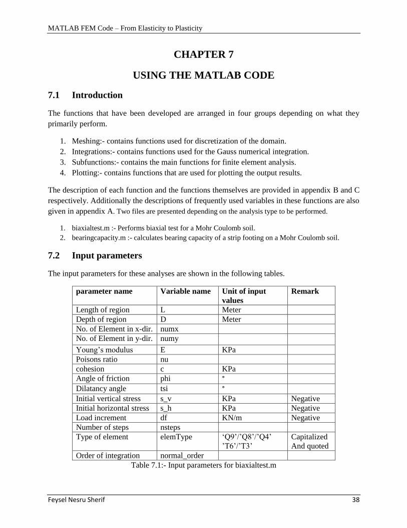
7.2 Input parameters

The input parameters for these analyses are shown in the following tables.

parameter name Variable name Unit of input

values

Remark

Length of region L Meter

Depth of region D Meter

No. of Element in x-dir. numx

No. of Element in y-dir. numy

Young‟s modulus E KPa

Poisons ratio nu

cohesion c KPa

Angle of friction phi °

Dilatancy angle tsi °

Initial vertical stress s_v KPa Negative

Initial horizontal stress s_h KPa Negative

Load increment df KN/m Negative

Number of steps nsteps

Type of element elemType „Q9‟/‟Q8‟/‟Q4‟

‟T6‟/‟T3‟

Capitalized

And quoted

Order of integration normal_order

Table 7.1:- Input parameters for biaxialtest.m



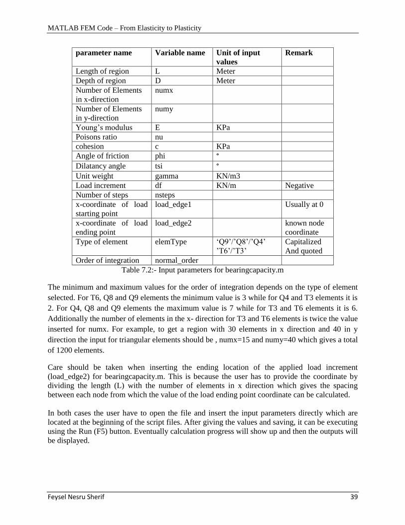
parameter name Variable name Unit of input

values

Remark

Length of region L Meter

Depth of region D Meter

Number of Elements

in x-direction

numx

Number of Elements

in y-direction

numy

Young‟s modulus E KPa

Poisons ratio nu

cohesion c KPa

Angle of friction phi °

Dilatancy angle tsi °

Unit weight gamma KN/m3

Load increment df KN/m Negative

Number of steps nsteps

x-coordinate of load

starting point

load_edge1

Usually at 0

x-coordinate of load

ending point

load_edge2

known node

coordinate

Type of element elemType „Q9‟/‟Q8‟/‟Q4‟

‟T6‟/‟T3‟

Capitalized

And quoted

Order of integration normal_order

Table 7.2:- Input parameters for bearingcapacity.m

The minimum and maximum values for the order of integration depends on the type of element

selected. For T6, Q8 and Q9 elements the minimum value is 3 while for Q4 and T3 elements it is

2. For Q4, Q8 and Q9 elements the maximum value is 7 while for T3 and T6 elements it is 6.

Additionally the number of elements in the x- direction for T3 and T6 elements is twice the value

inserted for numx. For example, to get a region with 30 elements in x direction and 40 in y

direction the input for triangular elements should be , numx=15 and numy=40 which gives a total

of 1200 elements.

Care should be taken when inserting the ending location of the applied load increment

(load_edge2) for bearingcapacity.m. This is because the user has to provide the coordinate by

dividing the length (L) with the number of elements in x direction which gives the spacing

between each node from which the value of the load ending point coordinate can be calculated.

In both cases the user have to open the file and insert the input parameters directly which are

located at the beginning of the script files. After giving the values and saving, it can be executing

using the Run (F5) button. Eventually calculation progress will show up and then the outputs will

be displayed.



7.3 Outputs

The outputs of the analysis are displayed automatically when the calculation is finished. The

default way of displaying the calculation results is in picture form these are:-

The finite element mesh.

The deformed finite element mesh

Displacement shadings (u_x and u_y)

Stress shadings (σxx, σyy, τxy and σzz )

Deviatoric stress vs. mean stress plot.

Vertical stress vs. vertical strain plot.

Deviatoric stress vs. volumetric strain plot.

Load vs. vertical displacement plot.

The mesh and the shading diagrams show the overall property of the domain while the curves are

plotted for a stress point in the element at the upper left corner. In this element the first gauss

point is selected as a stress point for rectangular elements and the third gauss point in triangular

elements. Examples of outputs from a bearing capacity problem are shown in chapter 8, pages

49-53.

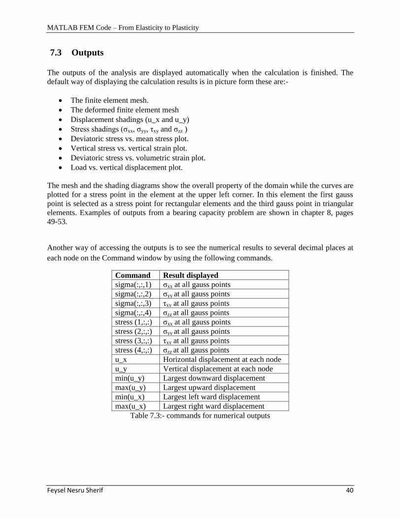
Another way of accessing the outputs is to see the numerical results to several decimal places at

each node on the Command window by using the following commands.

Command Result displayed

sigma(:,:,1) σxx at all gauss points

sigma(:,:,2) σyy at all gauss points

sigma(:,:,3) τxy at all gauss points

sigma(:,:,4) σzz at all gauss points

stress (1,:,:) σxx at all gauss points

stress (2,:,:) σyy at all gauss points

stress (3,:,:) τxy at all gauss points

stress (4,:,:) σzz at all gauss points

u_x Horizontal displacement at each node

u_y Vertical displacement at each node

min(u_y) Largest downward displacement

max(u_y) Largest upward displacement

min(u_x) Largest left ward displacement

max(u_x) Largest right ward displacement

Table 7.3:- commands for numerical outputs



In table 7.3 both sigma and stress shows the stresses at the gauss points but in a different manner.

sigma(:,:,:)

The first position is the element number which is between 1 and number of elements in the

domain. The second position is the gauss point number which is between 1 and kk (the number

of gauss points in the element). The third position is the stress name as shown in the table

above.For example sigma(4,1,2) displays the value of σyy for the first gauss point in the fourth

element.

stress(:,:,:)

The first position is the stress name as shown in the table above. The second position is the gauss

point number which is between 1 and kk (the number of gauss points in the element). The third

position is element number which is between 1 and number of elements in the domain. For

example stress(2,1,4) displays the value of σyy for the first gauss point in the fourth element.



CHAPTER 8

VERIFICATION AND CONCLUSION

8.1 Introduction

Now all the required functions developed, it is time to see the results and compare these results

with values from theoretical solutions and the PLAXIS software. For this purpose two types of

problem sets are discussed, biaxial test and bearing capacity problem.

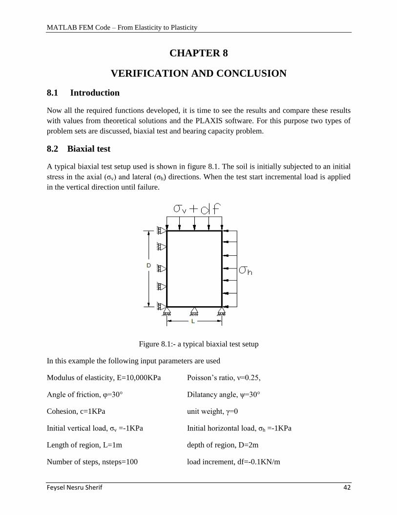
8.2 Biaxial test

A typical biaxial test setup used is shown in figure 8.1. The soil is initially subjected to an initial

stress in the axial (σv) and lateral (σh) directions. When the test start incremental load is applied

in the vertical direction until failure.

Figure 8.1:- a typical biaxial test setup

In this example the following input parameters are used

Modulus of elasticity, E=10,000KPa Poisson‟s ratio, ν=0.25,

Angle of friction, υ=30° Dilatancy angle, ψ=30°

Cohesion, c=1KPa unit weight, γ=0

Initial vertical load, σv =-1KPa Initial horizontal load, σh =-1KPa

Length of region, L=1m depth of region, D=2m

Number of steps, nsteps=100 load increment, df=-0.1KN/m



The theoretical solution for the failure load, according to Mohr Coulomb failure criteria is given

by,

1 2

1 sin cos2

1 sin 1 sinc

……………………..8.1

1

1 sin30 cos301* 2*1* 6.464

1 sin30 1 sin30KPa

In the Matlab code the above problem is solved using different combinations of element types

and numbers. The results are summarized in table 8.1

Element

type

numx=3 and numy=4 numx=5 and numy=6

σyy (KPa) u_y (mm) σyy (KPa) u_y (mm)

Q4, Q9, T6 -6.4 -2.7 -6.4 -2.4

Q8 -6.4 -2.8 -6.4 -2.8

T3 -6.4 -2.6 -6.4 -2.4

Table 8.1:- results from Matlab code

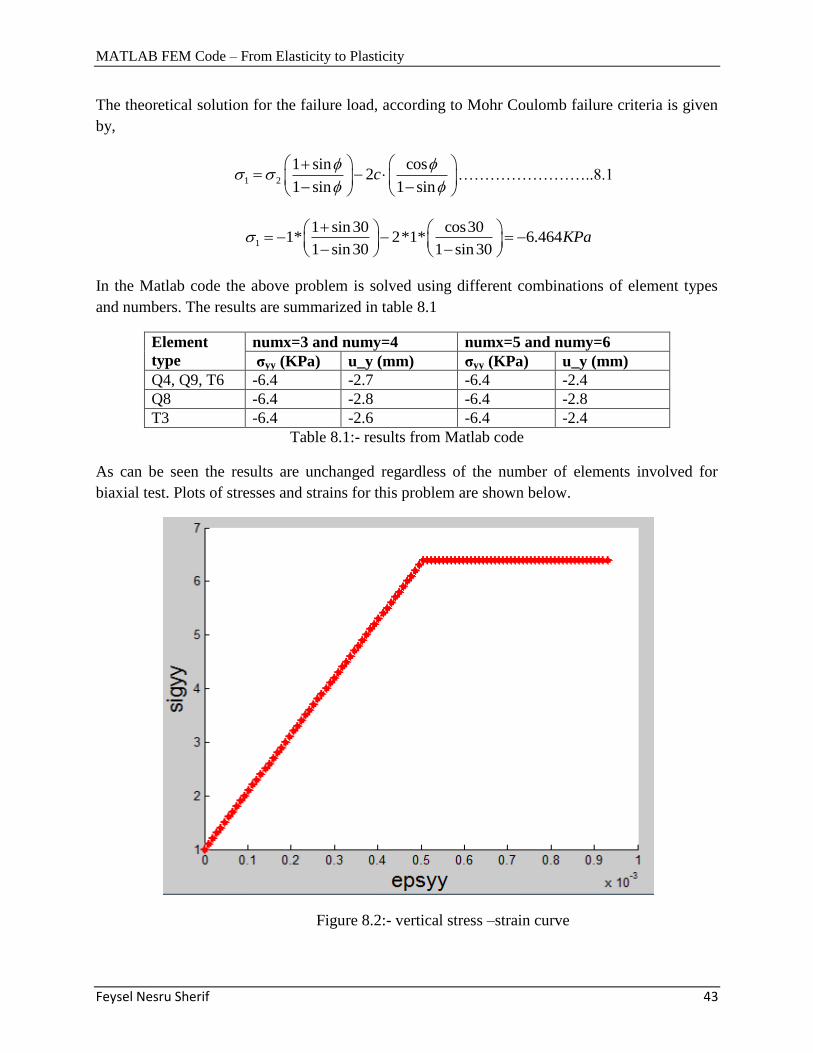
As can be seen the results are unchanged regardless of the number of elements involved for

biaxial test. Plots of stresses and strains for this problem are shown below.

Figure 8.2:- vertical stress –strain curve



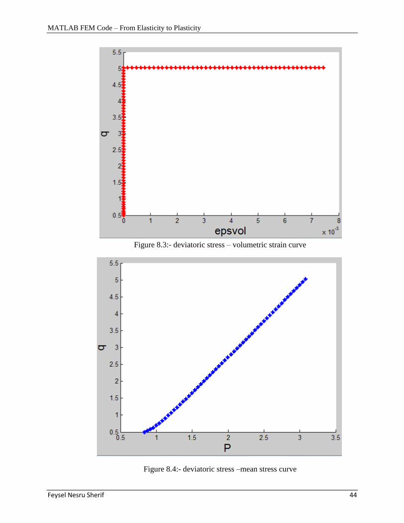
Figure 8.3:- deviatoric stress – volumetric strain curve

Figure 8.4:- deviatoric stress –mean stress curve



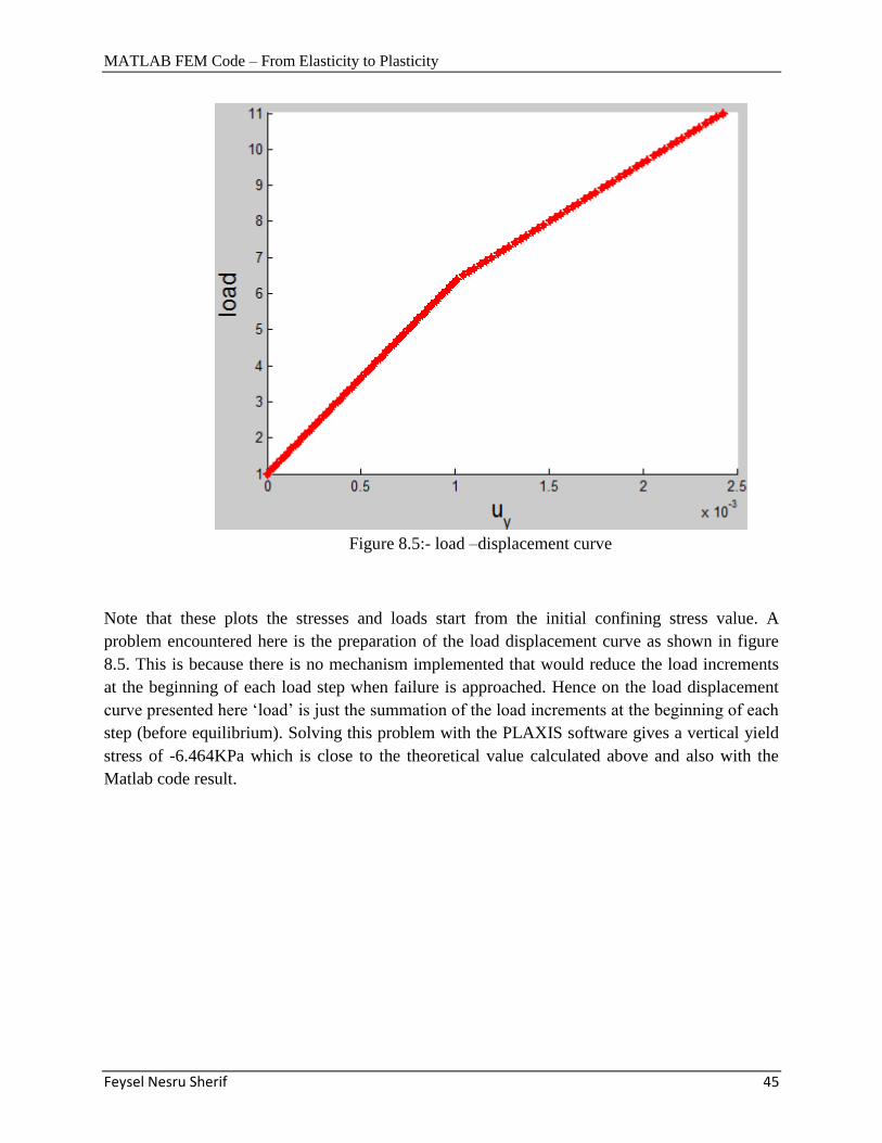
Figure 8.5:- load –displacement curve

Note that these plots the stresses and loads start from the initial confining stress value. A

problem encountered here is the preparation of the load displacement curve as shown in figure

8.5. This is because there is no mechanism implemented that would reduce the load increments

at the beginning of each load step when failure is approached. Hence on the load displacement

curve presented here „load‟ is just the summation of the load increments at the beginning of each

step (before equilibrium). Solving this problem with the PLAXIS software gives a vertical yield

stress of -6.464KPa which is close to the theoretical value calculated above and also with the

Matlab code result.



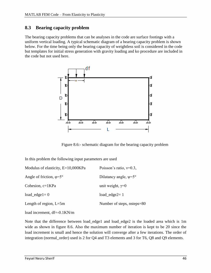
8.3 Bearing capacity problem

The bearing capacity problems that can be analyses in the code are surface footings with a

uniform vertical loading. A typical schematic diagram of a bearing capacity problem is shown

below. For the time being only the bearing capacity of weightless soil is considered in the code

but templates for initial stress generation with gravity loading and ko procedure are included in

the code but not used here.

Figure 8.6:- schematic diagram for the bearing capacity problem

In this problem the following input parameters are used

Modulus of elasticity, E=10,000KPa Poisson‟s ratio, ν=0.3,

Angle of friction, υ=5° Dilatancy angle, ψ=5°

Cohesion, c=1KPa unit weight, γ=0

load_edge1= 0 load_edge2= 1

Length of region, L=5m Number of steps, nsteps=80

load increment, df=-0.1KN/m

Note that the difference between load_edge1 and load_edge2 is the loaded area which is 1m

wide as shown in figure 8.6. Also the maximum number of iteration is kept to be 20 since the

load increment is small and hence the solution will converge after a few iterations. The order of

integration (normal_order) used is 2 for Q4 and T3 elements and 3 for T6, Q8 and Q9 elements.



For a weightless soil, γ = 0, the ultimate bearing capacity of strip foundations has closed form

solutions according to Prandtl,

0

( 2) 0

c

u

c N forq

c for

…………………….8.2

Where

Nc is a bearing capacity factor given by,

( 1)cotc qN N ………………………….8.3

While, tan 1 sin

1 sinqN e

………………….8.4

For the soil parameters given above the bearing capacity of the soil using equation 8.2 will be

1*6.489 6.489u cq c N KPa

This problem is first solved using the Matlab code for different domain depth (D) using a Q4

element. Keeping the number of element constant (numx=30 and numy=80) and varying the

depth for a 5m long region gave the following results.

Depth (m) Bearing capacity (KPa) 3 5.63

4 6.055

6 6.289

Table 8.2:- comparison of bearing capacity values for different depth of region

From these results it can be seen that for an accurate result the dimension of the region should be

sufficiently large. Hence for a footing with a width B, the length of the region should be at least

5*B and the depth should be 4*B. for the proceeding calculations a region 5m long a 6m deep is

used. Since the stress shadings and plots does not show these values with such precision, they

can be seen in Matlab by typing stress(:,:,ule) in the command window. The term ule refers to

the element at the left top corner and this element‟s gauss point is the stress point selected for

plotting the curves.



For comparison of results for different element types the number of elements is set to be 1200

and the dimension of the region 5m x 6m (L x D). The results are shown in table 8.3.

Element type numx numy Bearing capacity (KPa)

Q4 30 40 6.167

T3 15 40 5.943

T6 15 40 6.41

Q8 30 40 6.403

Q9 30 40 6.4023

Table 8.3:- comparison of bearing capacity values for different element types

As can be seen from these results, higher order elements (T6, Q8 and Q9 with normal_order =3 )

give a more accurate result than those of primary elements (T3 and Q4 with normal_order = 2).

In the primary elements the number of elements can be increased beyond 1200, for example, for

a Q4 element increasing the number of elements to 3200 (numx = 40 and numy = 80) gives a

bearing capacity of 6.388KPa which is still less accurate than those of the higher order types

with 1200 elements. For the case of higher order elements increasing the number of elements is

possible but restricted by the computer memory allocated for MATLAB.

Solving this same problem in the PLAXIS software using T6 elements with fine mesh gives a

bearing capacity value of 6.5113KPa. Hence the value from the Matlab code is close to both the

closed form solution and the PLAXIS software. A problem encountered in the bearing capacity

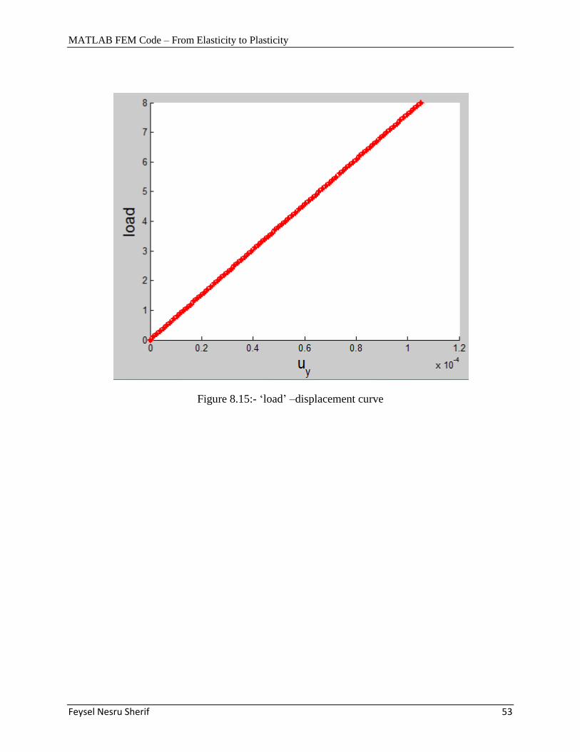
problem is the preparation of the load displacement curve as in the case of the biaxial test. This is

because there is no mechanism implemented that would reduce the load increments at the

beginning of each load step when failure is approached. Hence on the load displacement curve

presented here „load‟ is just the summation of the load increments at the beginning of each step

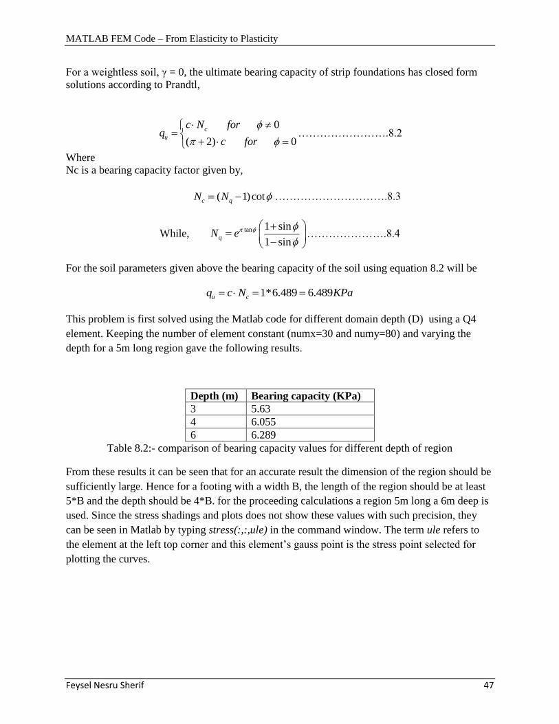
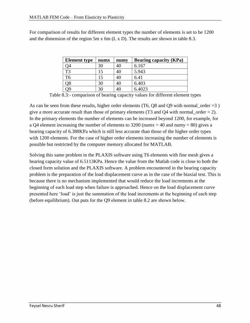
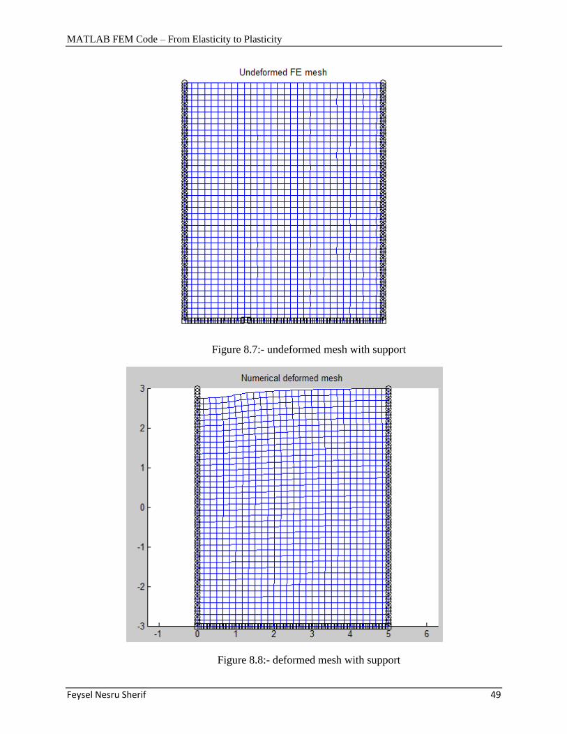
(before equilibrium). Out puts for the Q9 element in table 8.2 are shown below.



Figure 8.7:- undeformed mesh with support

Figure 8.8:- deformed mesh with support



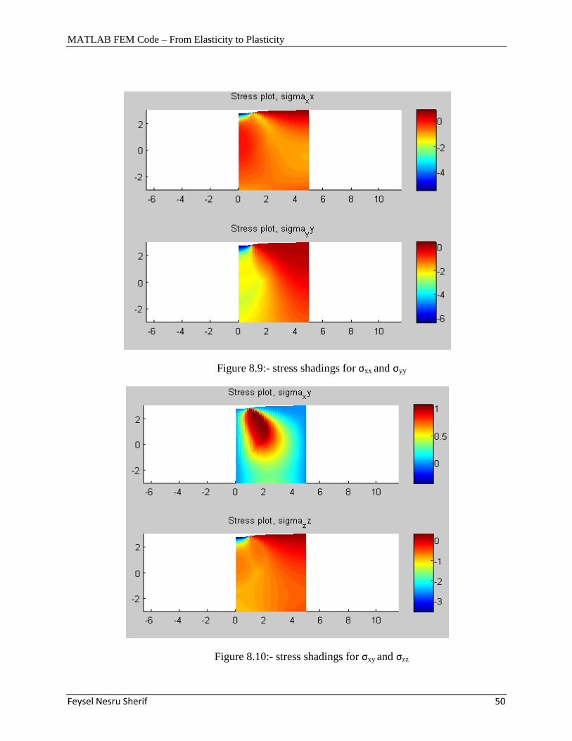
Figure 8.9:- stress shadings for σxx and σyy

Figure 8.10:- stress shadings for σxy and σzz



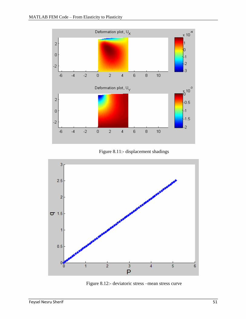
Figure 8.11:- displacement shadings

Figure 8.12:- deviatoric stress –mean stress curve



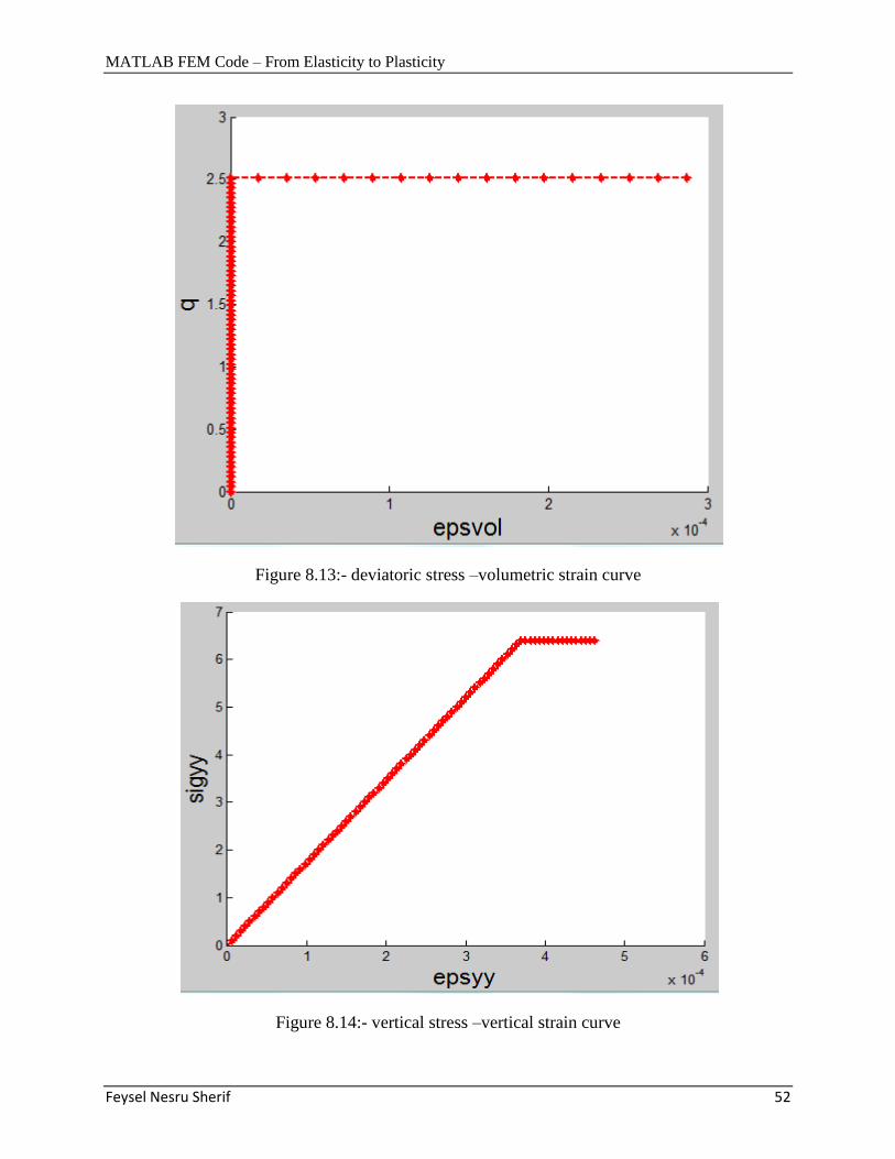
Figure 8.13:- deviatoric stress –volumetric strain curve

Figure 8.14:- vertical stress –vertical strain curve



Figure 8.15:- „load‟ –displacement curve



8.4 Conclusion

As can be seen from the above problems the accuracy of results is dependent on

The type of element

The number of elements and

For bearing capacity problems the dimension of the domain

Elementary element types (Q4 and T3) with an order of integration of 2 give a less accurate

result when compared to higher order element type (T6, Q8 and Q9) with an order of integration

of 3 for a given number of elements. Increasing the number of elements in elementary element

types makes the result more accurate, similarly increasing the number of elements has the same

effect on higher order elements but the time it takes for analysis is too long and takes too much

memory and usually results “out of memory” message from MATLAB due to the large size of

the stiffness matrix. The integration order used for the above problems is only the minimum

values but increasing it could make the results more accurate especially in higher order elements

when great accuracy is intended. But in the present case it would not make any difference except

slowing down the calculation.

In bearing capacity calculation, results are highly dependent on the dimensions of the domain

compared to that of the loaded area, the larger the dimensions the more accurate is the result.

Allocating a domain length, L, of five times the load span and a depth, D, of four times the load

span gave a good result in the above calculations. Another issue is the number of steps and the

size of load increment to be used, since both have to be inserted as an input. When the number of

steps is under estimated the soil will not reach at its plastic state and the analysis will be elastic.

Therefore it is advisable to make the number of steps large when the load increment is small.

Due to the explicit nature of the integration used in the code, it is strongly recommended to use a

small load increment. When solving a problem, it is advisable to start using the Q4 element with

an integration order of 2 for a quick and rough calculation and to see if the number of steps is

large enough, after which higher order elements with a larger integration order can be employed

for a fine and accurate result.



CHAPTER 9

SUMMARY AND FUTURE WORK

9.1 Summary

From the calculations in the previous chapter, it is seen that higher order elements are more

accurate than that of the elementary element types. A larger number of elements also improves

the accuracy of results. One shortcoming in the code is there is no algorithm for the reduction of

externally applied loads as failure is approached, which makes the load increment constant

before and after the onset of plasticity. This problem made the plotting of the actual load

displacement curve impossible. Instead the load displacement curve presented here is just the

sum of the load increments at the beginning of each load step.

9.2 Future Work

In the future, this code can be expanded to include other geotechnical problems like

Earth pressure calculations.

Slope stability and

Consolidation.



References

A.J.M. Ferreira

MATLAB Codes for Finite Element Analysis,Solids and Structures, Universidade do Porto

Portugal, Springer Science +Business Media B.V, 2009

Carlos A. Felippa, Introduction to Finite Element Methods,University of Colorado

Boulder, Colorado, USA, 2004

David M. Potts and Lidija Zdravkovic‟, Finite element analysis in geotechnical engineering:

Theory, Thomas Telford Ltd, London 1999

David M. Potts and Lidija Zdravkovic‟, Finite element analysis in geotechnical engineering:

Application, Thomas Telford Ltd, London 2001

D. M. Potts, Numerical analysis: a virtual dream or practical reality?

Ge´otechnique 53, No. 6, 535–573, 2003

D. V. Griffiths and S.M. Willson, An explicit form of the plastic matrix for a Mohr-Coulomb

material, communications in applied numerical methods, vol. 2, 523-529 (1986)

Dr James P Doherty, Introducing plasticity into the finite element method,

Computational Geomechanics (CIVIL8120) Notes, The University of Western Australia

School of Civil and Resources Engineering, 2010

Klaus-Jurgen Bathe, Finite Element Procedures, Prentice-Hall Inc., 1996

O.C. Zienkiewicz and R.L. Taylor, The Finite Element Method for Solid and Structural

Mechanics, Elsevier Butterworth-Heinemann, oxford, 6th edition, 2005.

PLAXIS. Plaxis 2D - Version 10. Plaxis bv, Delft, The Netherlands, 2010.

PLAXIS, validation and verification, Plaxis bv, Delft, The Netherlands, 2011.

S.S Bhavikatti, Finite Element Analysis, New Age International (P) Ltd. Publishers, 2005

Singiresu S. Rao, The Finite Element Method in Engineering, 4th

edition, Elsevier Science and

Technology Books, 2004

Dr Stephano Dal Pont, David Noel, Sundararajan Natatajan, Dr Stephane PA Bordas, Extended

Finite Element and Flexible Finite Element Method MATLAB Toolbox, 2008

Yingren Zheng, Xiaosong Tang, Shangyi Zhao, Chujian Deng, Wenjie Lei

Strength reduction and step-loading finite element approaches in geotechnical engineering

Journal of Rock Mechanics and Geotechnical Engineering. 2009, 1 (1): 21–30

A1

Appendix A

Variable Nomenclature

Bfem:- the strain displacement matrix.

botEdge :- nodes along bottom edge of the domain in pairs

botNodes :- nodes along bottom edge of the domain

C: - The elastic compliance matrix.

coord:- matrix of the coordinates of the gauss points in the natural coordinate system.

CP: - The plastic compliance matrix.

dispNodes :- nodes which are restrained from displacement in any direction.

dispNodes1:- nodes which are restrained from displacement in x-direction.

dNdxi:- matrix of the derivative of the shape function.

dof:- vector of the total degree of freedom.

E:-modulus of elasticity

eldof:- matrix containing the degree of freedom in an element

element :– a matrix that contains the node id in each element.

Elements: – a matrix that contains the node id in each element for Q8 or Q9 element before

rearranged in the final manner.

elemType:- the type of element selected.

eta:- the natural y coordinate of the gauss points.

F: - the force matrix

f:- the externally applied force matrix.

F:- the total load (the sum of external load and self weight).

fac:- magnification factor for plotting outputs.

field:- a command for the output data to be plotted in color shading.

gamma :- self weight of soil.

iel:- a counter running from 1 up to the number of elements in the region.

inc_u:- the node counting increment in x direction (default=1)

inc_v:- the node counting increment in y direction

invJ0:- inverse of Jacobian matrix.

J0:- Jacobian matrix.

A2

K: - the global stiffness matrix.

kk:- a counter running from 1 up to the number of gauss points in the element.

L, D: - Dimensions of the region in x and y direction respectively.

leftEdge :- nodes along left edge of the domain in pairs

leftNodes :- nodes along left edge of the domain

leftNodes1:- nodes along left edge of the domain except the lower left node.

lln :- lower left node

load_edge1:- the x-coordinate of the node at which the externally applied load starts.

load_edge2:- the x-coordinate of the node at which the externally applied load ends.

lrn :- lower right node

N:-shape function vector.

nn:- number of nodes in an element.

nnx:- number of nodes in the x direction.

nny:- number of nodes in the y direction.

node :- matrix that contains the coordinate of the nodes.

node_pattern:- counting order of nodes arranged numerically.

Nodes :- matrix that contains the coordinate of the nodes for Q8 or Q9 element before rearranged

in the final manner.

nonelem:- number of gauss points in an element.

normal_order :- number of gauss integration points (order of integration).

nu :- Poisson's ratio

numberelem:- total number of elements in the domain for a T3 or T6 element.

numelem:- number of elements in the region.

numnode:- total number of nodes in the region.

numx:- number of elements in the x direction.

numy:- number of elements in the y direction.

pt1, pt2, pt3, pt4:- coordinates of the corner points of the domain.

Q: - coordinates matrix of the gauss integration points.

qt:- type of integration to be done.

quadorder :-number of gauss integration points.

rightEdge :- nodes along right edge of the domain in pairs

A3

rightNodes :- nodes along right edge of the domain

rightNodes1:- nodes along right edge of the domain except the lower right node.

sdim:- coordinate dimension of element for gauss integration either line element (value=1) of

plane element (value=2).

se:- plotting color for the finite element mesh (default ‘blue’)

selfwt:- the self weight matrix.

sigmatox :- externally applied horizontal load.

sigmatoy :- externally applied vertical load.

Stresspoints:- nodes at which the stress is calculated.

topEdge :- nodes along the top edge of the domain in pairs

topEdge1:- nodes along the top edge of the domain in triples for Q9,Q8 and T6 elements.

topNodes :- nodes along the top edge of the domain

total_unknown:- the total degree of freedom in the domain.

type:-the type of element selected for shape function calculation.

U:- nodal displacements.

u_x:- nodal displacements in x-direction.

u_y:- nodal displacements in y-direction.

udof:- vector of the horizontal degree of freedom.

ule :- upper left element.

uln :- upper left node.

urn :- upper right node.

vdof:- vector of the vertical degree of freedom.

W: - vector of weight for the gauss integration.

xi:- the natural x coordinate of the gauss points.

xx:- a vector of x coordinates of nodes for a T6 element.

yy:- a vector of y coordinates of nodes for a T6 element.

B1

Appendix B

Function Description

square_node_array:- Generates a quadrilateral array of nodes between the counterclockwise

ordering of nodes pt1 - pt4.

Inputs: - pt1, pt2, pt3, pt4, nnx, nny.

Outputs: - node

q4totq8:- Forms the element and node matrices for Q8 element, from the element and node

matrices of a Q4 element with the element and node matrices arranged in a counterclockwise

order.

Inputs:-element, node, numx, numy.

Outputs: - Elements, Nodes

q4totq9:- Forms the element and node matrices for nine Q9 element, from the element and node

matrices of a Q4 element with the element and node matrices arranged in a numerical

counterclockwise order.

Inputs:-element, node, numx, numy.

Outputs: - Elements, Nodes

structured_q8_mesh:- Forms the element and node matrices for Q8 element, with the element

and node matrices arranged in a nodal counterclockwise order (primary nodes then secondary

nodes)

Inputs: - pt1, pt2, pt3, pt4, numx, numy.

Outputs: - node, element

structured_q9_mesh:- Forms the element and node matrices for Q9 element, with the element

and node matrices arranged in a nodal counterclockwise order (primary nodes-> secondary nodes

then internal nodes)

Inputs: - pt1, pt2, pt3, pt4, numx, numy.


make_elem:- creates a connectivity list of primary nodes in Q4 and T3 element.

Inputs: - node_pattern, numx, numy, inc_u, inc_v

Outputs: - element

mesh_region:- switching the element type selected, it forms the final nodal and element

connectivity.using the above six functions for Q4, Q8, Q9 and T3 element.

Inputs: - pt1, pt2, pt3, pt4, numx, numy, elemType


B2

mesh_t6_elem:- Forms the element and node matrices for T6 element, with the element and

node matrices arranged in a nodal counterclockwise order (primary nodes then secondary nodes).

Inputs: - L, D, numx, numy


supportcond:- Forms a vector of nodes which are restrained in x direction or in both x and y

direction which are the supports of the domain. It also forms a matrix of nodes for load

application at the top of the domain.

Inputs: - elemType, numx, numy

Outputs: - topEdge, topEdge1, dispNodes, dispNodes1, leftNodes1

elementdof:- Forms the global degree of freedom nodes in each element from the node

identification number.

Inputs: - elemType, sctr

Outputs: - eldof

gauss_pt_wt:- Returns the weights and coordinates of the gauss integration points.

Inputs: - quadorder, qt, sdim

Outputs: - W, Q

gauss_rule:- Provides the weight vector and gauss point coordinate matrix of the element based

on the integration order selected.

Inputs: - iel, elemType, normal_order

Outputs: - W, Q

shape_func:- Gives the shape function and its derivatives with respect to x and y.

Inputs: - type, coord, dim

Outputs: - N, dNdxi

Bmatrix:- Gives the strain displacement matrix (B matrix size 3x8) for each element.

Inputs: - pt, elemType, iel

Outputs: - Bfem

Bmatrix4:- Gives the strain displacement matrix (B matrix size 4x8) for each element.

Inputs: - pt, elemType, iel

Outputs: - Bfem4

B3

stiffness_matrix:- Generates the element and global stiffness matrix.

Inputs: - node, element, elemType, normal_order, C

Outputs: - K

force_matrix:- Generates the force matrix due to externally applied loads for Q4 and T3

elements and the position of the vertically applied load (sctry) in the global degree of freedom.

Inputs: - node, topEdge, sigmatoy, sigmatox, load_edge1, load_edge2, D

Outputs: - f, sctry

force_matrix689:- Generates the force matrix due to externally applied loads for Q9, Q8 and T6

elements and the position of the vertically applied load (sctry) in the global degree of freedom.

Inputs: - node, topEdge, topEdge1, sigmatoy, sigmatox, load_edge1, load_edge2, D

Outputs: - f, sctry

selfwt_matrix:- Generates the force matrix due to self weight.

Inputs: - elemType, normal_order, gamma, node, element

Outputs: - selfwt

displacements:- evaluates the unknown degree of freedom (displacements) at the nodes.

Inputs: - dispNodes, dispNodes1, numnode, K, f, selfwt

Outputs: - U, u_x, u_y

stress_calculation:- calculates the element strains and stresses at the nodes in x, y, xy and zz

directions.

Inputs: - node, element, elemType, U, normal_order, C

Outputs: - stress, strain

invariants:- calculates the stress invariants for a single gauss point.

Inputs: - stress

Outputs: - p, q, theta

invariants1:- calculates the stress invariants at each gauss point. This can be used outside the

iteration loop.

Inputs: - element, stress


invariants2:- calculates the stress invariants at each gauss point. This can be used inside the

iteration loop.

Inputs: - kk, iel, stress


B4

formdg:- calculates the partial derivatives of the plastic potential with respect to p, J2 and J3.

Inputs: - tsi, q, theta

Outputs: - dg1, dg2, dg3

formdm:- Generates the partial derivatives of the p, J2 and J3 with respect to stress for use in the

plastic potential derivative.

Inputs: - kk, iel, stress

Outputs: - m1, m2, m3

internalrxn:- Generates the vector of nodal force reactions due to internal stress. It can be used

outside the iteration loop if the stress at each gauss point is given.

Inputs: - node, element, elemType, normal_order, stress

Outputs: - r

principal_stress:- calcualtes the principal stresses from the stress invariants.

Inputs: - kk, iel, p, q, theta

Outputs: - s1, s2, s3

plastic_mat:- Generates the plastic constitutive matix CP at each gauss point.

Inputs: - E, nu, phi, tsi, iel, kk, stress

Outputs: - CP

makedgds:- Forms the partial derivatives of the plastic potential function with respect to stress at

each gauss point.

Inputs: - tsi, element, iel, kk, stress

Outputs: - dgds

makedfds:- Forms the partial derivatives of the yield function with respect to stress at each

gauss point.

Inputs: - phi, element, iel, kk, stress

Outputs: - dfds

plot_mesh:- Plots the finite element mesh

Inputs: - node, connect, elem_type, se

Outputs: - plot

plot_m:- Plots the finite element mesh with the support condition.

Inputs: - elemType, dispNodes, dispNodes1

Outputs: - plot

plot_def:- Plots the deformed finite element mesh with the support condition.

Inputs: - fac, u_x, u_y, elemType, dispNodes, dispNodes1

Outputs: - plot

B5

plot_field:- Forms a color dependent finite element mesh for plotting outputs

Inputs: - node, connect, elem_type, field

Outputs: - plot

plot_sig:- plots the color coded stress distribution in the finite element region along with color

bar scale.

Inputs: - fac, u_x, u_y, elemType, stress

Outputs: - plot

plot_defo:- plots the color coded displacement intensity in the finite element region along with

color bar scale.

Inputs: - fac, u_x, u_y, elemType

Outputs: - plot

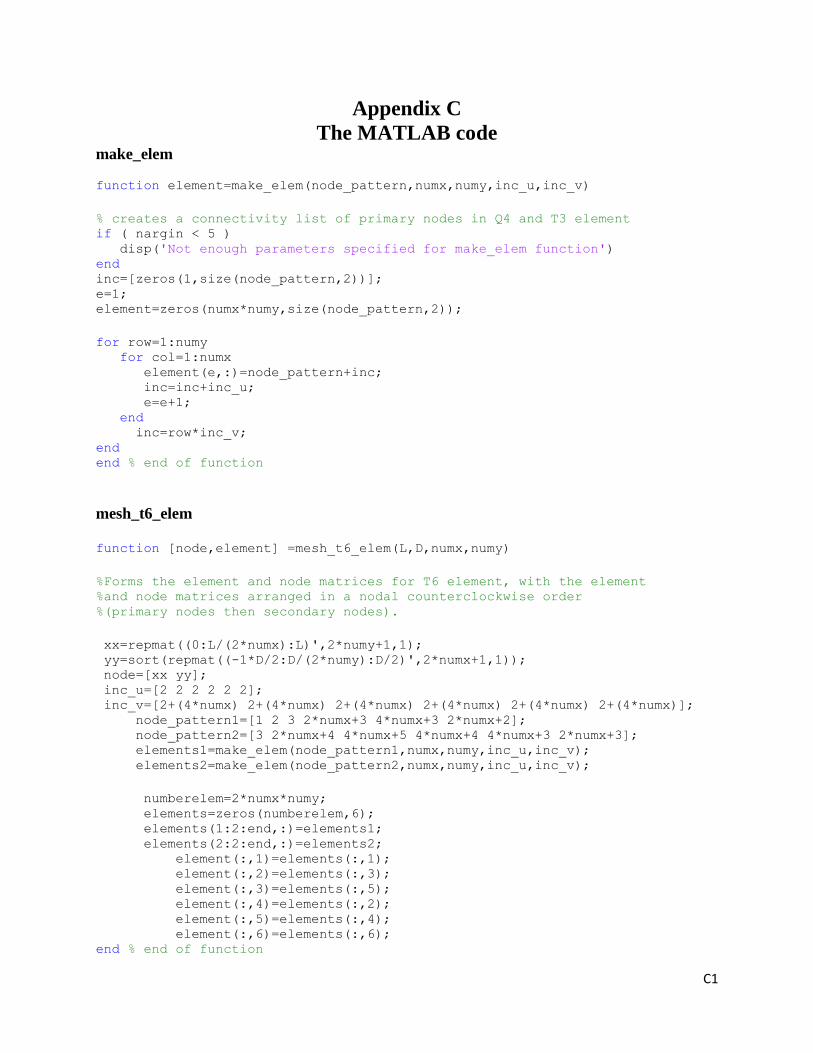
C1

Appendix C

The MATLAB code make_elem

function element=make_elem(node_pattern,numx,numy,inc_u,inc_v)

% creates a connectivity list of primary nodes in Q4 and T3 element if ( nargin < 5 ) disp('Not enough parameters specified for make_elem function') end inc=[zeros(1,size(node_pattern,2))]; e=1; element=zeros(numx*numy,size(node_pattern,2));

for row=1:numy for col=1:numx element(e,:)=node_pattern+inc; inc=inc+inc_u; e=e+1; end inc=row*inc_v; end end % end of function

mesh_t6_elem

function [node,element] =mesh_t6_elem(L,D,numx,numy)

%Forms the element and node matrices for T6 element, with the element %and node matrices arranged in a nodal counterclockwise order %(primary nodes then secondary nodes).

xx=repmat((0:L/(2*numx):L)',2*numy+1,1); yy=sort(repmat((-1*D/2:D/(2*numy):D/2)',2*numx+1,1)); node=[xx yy]; inc_u=[2 2 2 2 2 2]; inc_v=[2+(4*numx) 2+(4*numx) 2+(4*numx) 2+(4*numx) 2+(4*numx) 2+(4*numx)]; node_pattern1=[1 2 3 2*numx+3 4*numx+3 2*numx+2]; node_pattern2=[3 2*numx+4 4*numx+5 4*numx+4 4*numx+3 2*numx+3]; elements1=make_elem(node_pattern1,numx,numy,inc_u,inc_v); elements2=make_elem(node_pattern2,numx,numy,inc_u,inc_v);

numberelem=2*numx*numy; elements=zeros(numberelem,6); elements(1:2:end,:)=elements1; elements(2:2:end,:)=elements2; element(:,1)=elements(:,1); element(:,2)=elements(:,3); element(:,3)=elements(:,5); element(:,4)=elements(:,2); element(:,5)=elements(:,4); element(:,6)=elements(:,6); end % end of function

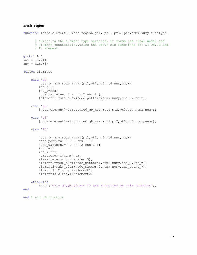
C2

mesh_region

function [node,element]= mesh_region(pt1, pt2, pt3, pt4,numx,numy,elemType)

% switching the element type selected, it forms the final nodal and

% element connectivity.using the above six functions for Q4,Q8,Q9 and

% T3 element.

global L D nnx = numx+1; nny = numy+1;

switch elemType

case 'Q4' node=square_node_array(pt1,pt2,pt3,pt4,nnx,nny); inc_u=1; inc_v=nnx; node_pattern=[ 1 2 nnx+2 nnx+1 ]; [element]=make_elem(node_pattern,numx,numy,inc_u,inc_v);

case 'Q9' [node,element]=structured_q9_mesh(pt1,pt2,pt3,pt4,numx,numy);

case 'Q8' [node,element]=structured_q8_mesh(pt1,pt2,pt3,pt4,numx,numy);

case 'T3'

node=square_node_array(pt1,pt2,pt3,pt4,nnx,nny); node_pattern1=[ 1 2 nnx+1 ]; node_pattern2=[ 2 nnx+2 nnx+1 ]; inc_u=1; inc_v=nnx; numberelem=2*numx*numy; element=zeros(numberelem,3); element1=make_elem(node_pattern1,numx,numy,inc_u,inc_v); element2=make_elem(node_pattern2,numx,numy,inc_u,inc_v); element(1:2:end,:)=element1; element(2:2:end,:)=element2;

otherwise error('only Q4,Q9,Q8,and T3 are supported by this function'); end

end % end of function

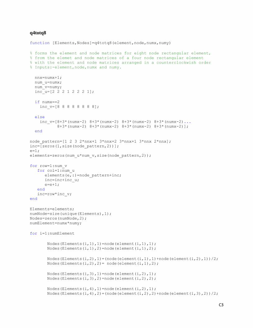
C3

q4totq8

function [Elements,Nodes]=q4totq8(element,node,numx,numy)

% forms the element and node matrices for eight node rectangular element, % from the elemet and node matrices of a four node rectangular element % with the element and node matrices arranged in a counterclockwish order % Inputs:-element,node,numx and numy.

nnx=numx+1; num_u=numx; num_v=numy; inc_u=[2 2 2 1 2 2 2 1];

if numx==2 inc_v=[8 8 8 8 8 8 8 8];

else inc_v=[8+3*(numx-2) 8+3*(numx-2) 8+3*(numx-2) 8+3*(numx-2)... 8+3*(numx-2) 8+3*(numx-2) 8+3*(numx-2) 8+3*(numx-2)]; end

node_pattern=[1 2 3 2*nnx+1 3*nnx+2 3*nnx+1 3*nnx 2*nnx]; inc=[zeros(1,size(node_pattern,2))]; e=1; elements=zeros(num_u*num_v,size(node_pattern,2));

for row=1:num_v for col=1:num_u elements(e,:)=node_pattern+inc; inc=inc+inc_u; e=e+1; end inc=row*inc_v; end

Elements=elements; numNode=size(unique(Elements),1); Nodes=zeros(numNode,2); numElement=numx*numy;

for i=1:numElement

Nodes(Elements(i,1),1)=node(element(i,1),1); Nodes(Elements(i,1),2)=node(element(i,1),2);

Nodes(Elements(i,2),1)=(node(element(i,1),1)+node(element(i,2),1))/2; Nodes(Elements(i,2),2)= node(element(i,1),2);


Nodes(Elements(i,4),1)=node(element(i,2),1); Nodes(Elements(i,4),2)=(node(element(i,2),2)+node(element(i,3),2))/2;

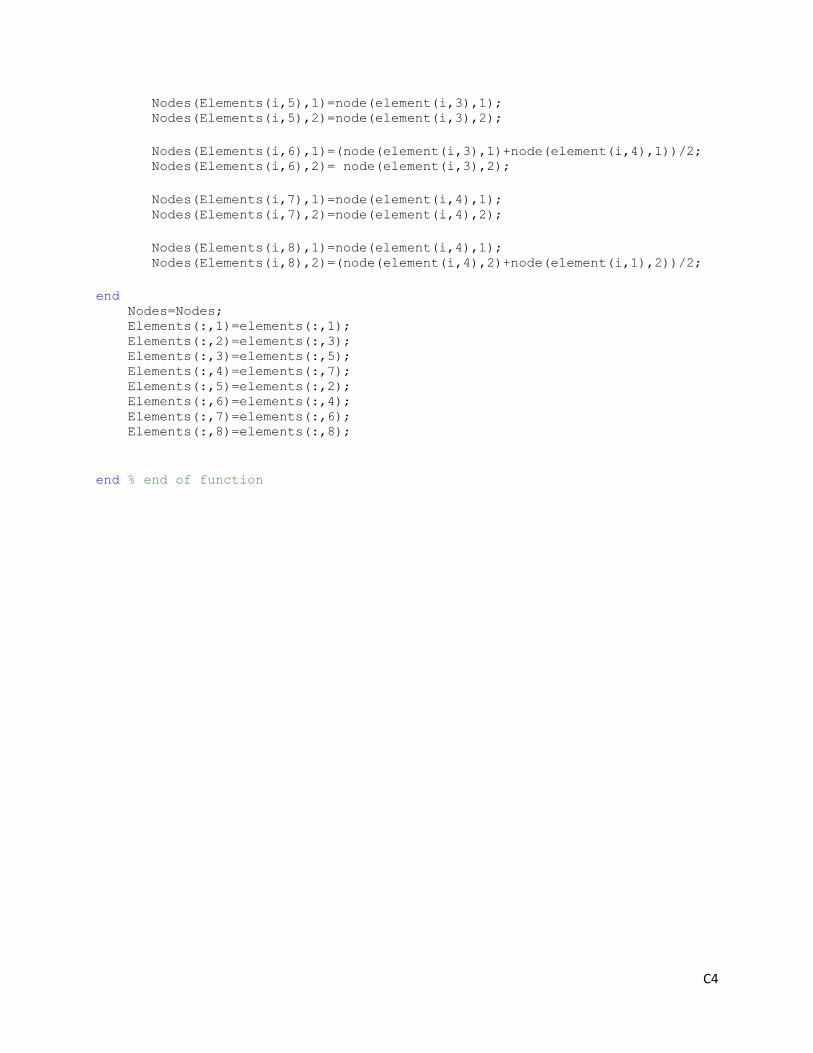
C4





end Nodes=Nodes; Elements(:,1)=elements(:,1); Elements(:,2)=elements(:,3); Elements(:,3)=elements(:,5); Elements(:,4)=elements(:,7); Elements(:,5)=elements(:,2); Elements(:,6)=elements(:,4); Elements(:,7)=elements(:,6); Elements(:,8)=elements(:,8);


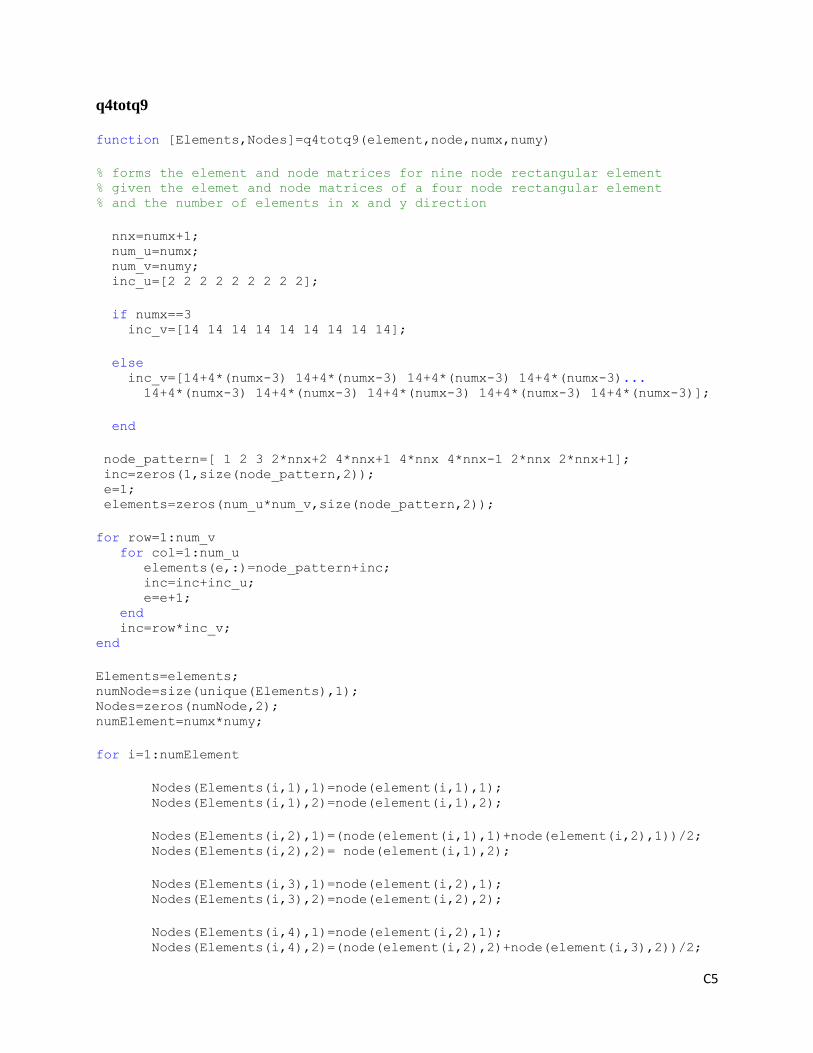
C5

q4totq9

function [Elements,Nodes]=q4totq9(element,node,numx,numy)

% forms the element and node matrices for nine node rectangular element % given the elemet and node matrices of a four node rectangular element % and the number of elements in x and y direction

nnx=numx+1; num_u=numx; num_v=numy; inc_u=[2 2 2 2 2 2 2 2 2];

if numx==3 inc_v=[14 14 14 14 14 14 14 14 14];

else inc_v=[14+4*(numx-3) 14+4*(numx-3) 14+4*(numx-3) 14+4*(numx-3)... 14+4*(numx-3) 14+4*(numx-3) 14+4*(numx-3) 14+4*(numx-3) 14+4*(numx-3)];

end

node_pattern=[ 1 2 3 2*nnx+2 4*nnx+1 4*nnx 4*nnx-1 2*nnx 2*nnx+1]; inc=zeros(1,size(node_pattern,2)); e=1; elements=zeros(num_u*num_v,size(node_pattern,2));

for row=1:num_v for col=1:num_u elements(e,:)=node_pattern+inc; inc=inc+inc_u; e=e+1; end inc=row*inc_v; end

Elements=elements; numNode=size(unique(Elements),1); Nodes=zeros(numNode,2); numElement=numx*numy;

for i=1:numElement





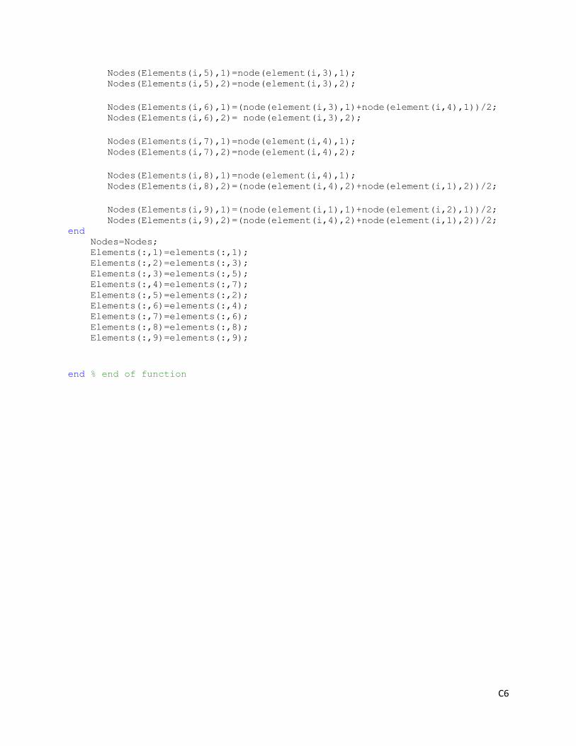
C6





Nodes(Elements(i,9),1)=(node(element(i,1),1)+node(element(i,2),1))/2; Nodes(Elements(i,9),2)=(node(element(i,4),2)+node(element(i,1),2))/2; end Nodes=Nodes; Elements(:,1)=elements(:,1); Elements(:,2)=elements(:,3); Elements(:,3)=elements(:,5); Elements(:,4)=elements(:,7); Elements(:,5)=elements(:,2); Elements(:,6)=elements(:,4); Elements(:,7)=elements(:,6); Elements(:,8)=elements(:,8); Elements(:,9)=elements(:,9);


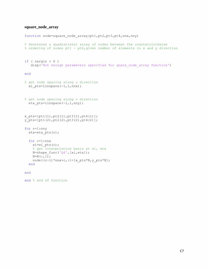
C7

square_node_array

function node=square_node_array(pt1,pt2,pt3,pt4,nnx,nny)

% Generates a quadratleral array of nodes between the counterclockwise % ordering of nodes pt1 - pt4,given number of elements in x and y direction

if ( nargin < 6 ) disp('Not enough parameters specified for quare_node_array function')

end

% get node spacing along u direction xi_pts=linspace(-1,1,nnx);

% get node spacing along v direction eta_pts=linspace(-1,1,nny);

x_pts=[pt1(1),pt2(1),pt3(1),pt4(1)]; y_pts=[pt1(2),pt2(2),pt3(2),pt4(2)];

for r=1:nny eta=eta_pts(r);

for c=1:nnx xi=xi_pts(c); % get interpolation basis at xi, eta N=shape_func('Q4',[xi,eta]); N=N(:,1); node((r-1)*nnx+c,:)=[x_pts*N,y_pts*N]; end

end


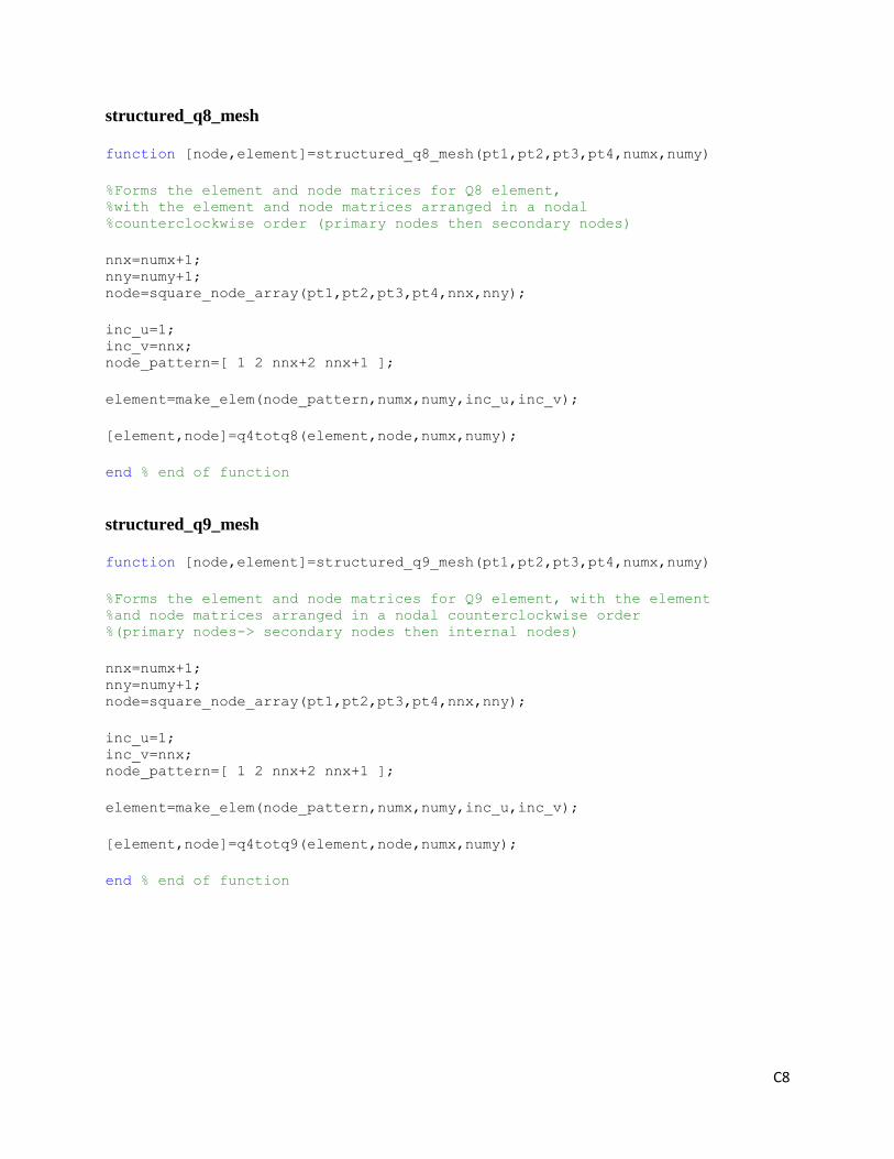
C8

structured_q8_mesh

function [node,element]=structured_q8_mesh(pt1,pt2,pt3,pt4,numx,numy)

%Forms the element and node matrices for Q8 element, %with the element and node matrices arranged in a nodal %counterclockwise order (primary nodes then secondary nodes)

nnx=numx+1; nny=numy+1; node=square_node_array(pt1,pt2,pt3,pt4,nnx,nny);

inc_u=1; inc_v=nnx; node_pattern=[ 1 2 nnx+2 nnx+1 ];

element=make_elem(node_pattern,numx,numy,inc_u,inc_v);

[element,node]=q4totq8(element,node,numx,numy);


structured_q9_mesh function [node,element]=structured_q9_mesh(pt1,pt2,pt3,pt4,numx,numy)

%Forms the element and node matrices for Q9 element, with the element %and node matrices arranged in a nodal counterclockwise order %(primary nodes-> secondary nodes then internal nodes)

nnx=numx+1; nny=numy+1; node=square_node_array(pt1,pt2,pt3,pt4,nnx,nny);

inc_u=1; inc_v=nnx; node_pattern=[ 1 2 nnx+2 nnx+1 ];

element=make_elem(node_pattern,numx,numy,inc_u,inc_v);

[element,node]=q4totq9(element,node,numx,numy);


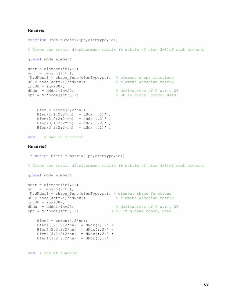
C9

Bmatrix

function Bfem =Bmatrix(pt,elemType,iel)

% Gives the strain displacement matrix (B matrix of size 3x8)of each element

global node element

sctr = element(iel,:); nn = length(sctr); [N,dNdxi] = shape_func(elemType,pt); % element shape functions J0 = node(sctr,:)'*dNdxi; % element Jacobian matrix invJ0 = inv(J0); dNdx = dNdxi*invJ0; % derivatives of N w.r.t XY Gpt = N'*node(sctr,:); % GP in global coord, used

Bfem = zeros(3,2*nn); Bfem(1,1:2:2*nn) = dNdx(:,1)' ; Bfem(2,2:2:2*nn) = dNdx(:,2)' ; Bfem(3,1:2:2*nn) = dNdx(:,2)' ; Bfem(3,2:2:2*nn) = dNdx(:,1)' ;


Bmatrix4

function Bfem4 =Bmatrix4(pt,elemType,iel)

% Gives the strain displacement matrix (B matrix of size 4x8)of each element

global node element

sctr = element(iel,:); nn = length(sctr); [N,dNdxi] = shape_func(elemType,pt); % element shape functions J0 = node(sctr,:)'*dNdxi; % element Jacobian matrix invJ0 = inv(J0); dNdx = dNdxi*invJ0; % derivatives of N w.r.t XY Gpt = N'*node(sctr,1); % GP in global coord, used

Bfem4 = zeros(4,2*nn); Bfem4(1,1:2:2*nn) = dNdx(:,1)' ; Bfem4(2,2:2:2*nn) = dNdx(:,2)' ; Bfem4(3,1:2:2*nn) = dNdx(:,2)' ; Bfem4(3,2:2:2*nn) = dNdx(:,1)' ;


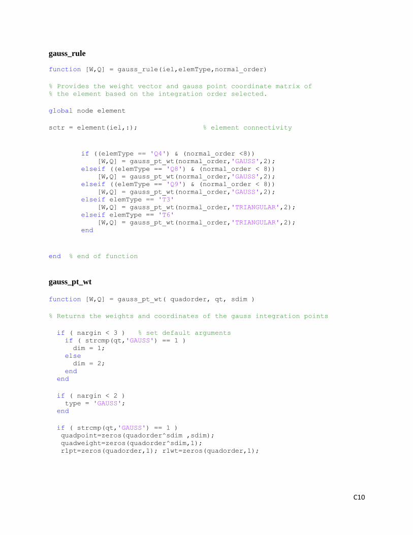
C10

gauss_rule

function [W,Q] = gauss_rule(iel,elemType,normal_order)

% Provides the weight vector and gauss point coordinate matrix of % the element based on the integration order selected.

global node element

sctr = element(iel,:); % element connectivity

if ((elemType == 'Q4') & (normal_order <8)) [W,Q] = gauss_pt_wt(normal_order,'GAUSS',2); elseif ((elemType == 'Q8') & (normal_order < 8)) [W,Q] = gauss_pt_wt(normal_order,'GAUSS',2); elseif ((elemType == 'Q9') & (normal_order < 8)) [W,Q] = gauss_pt_wt(normal_order,'GAUSS',2); elseif elemType == 'T3' [W,Q] = gauss_pt_wt(normal_order,'TRIANGULAR',2); elseif elemType == 'T6' [W,Q] = gauss_pt_wt(normal_order,'TRIANGULAR',2); end


gauss_pt_wt function [W,Q] = gauss_pt_wt( quadorder, qt, sdim )

% Returns the weights and coordinates of the gauss integration points

if ( nargin < 3 ) % set default arguments if ( strcmp(qt,'GAUSS') == 1 ) dim = 1; else dim = 2; end end

if ( nargin < 2 ) type = 'GAUSS'; end

if ( strcmp(qt,'GAUSS') == 1 ) quadpoint=zeros(quadorder^sdim ,sdim); quadweight=zeros(quadorder^sdim,1);

r1pt=zeros(quadorder,1); r1wt=zeros(quadorder,1);

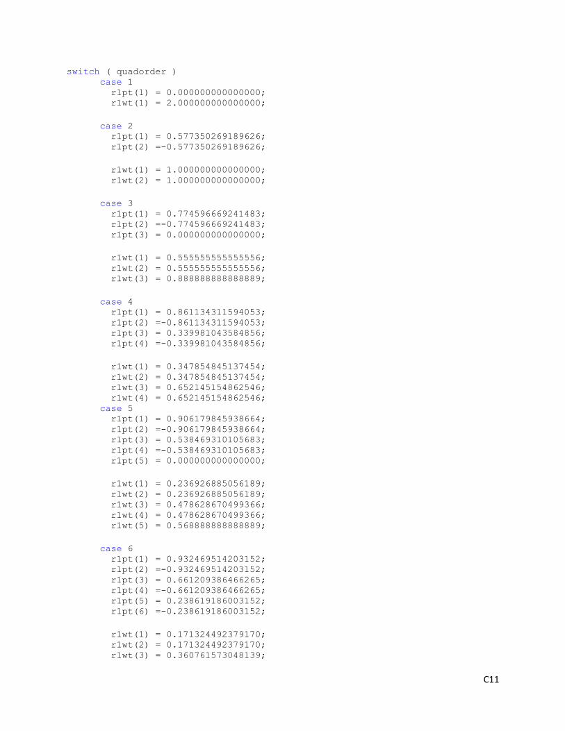
C11

switch ( quadorder ) case 1 r1pt(1) = 0.000000000000000; r1wt(1) = 2.000000000000000;

case 2 r1pt(1) = 0.577350269189626; r1pt(2) =-0.577350269189626;

r1wt(1) = 1.000000000000000; r1wt(2) = 1.000000000000000;

case 3 r1pt(1) = 0.774596669241483; r1pt(2) =-0.774596669241483; r1pt(3) = 0.000000000000000;

r1wt(1) = 0.555555555555556; r1wt(2) = 0.555555555555556; r1wt(3) = 0.888888888888889;

case 4 r1pt(1) = 0.861134311594053; r1pt(2) =-0.861134311594053; r1pt(3) = 0.339981043584856; r1pt(4) =-0.339981043584856;

r1wt(1) = 0.347854845137454; r1wt(2) = 0.347854845137454; r1wt(3) = 0.652145154862546; r1wt(4) = 0.652145154862546; case 5 r1pt(1) = 0.906179845938664; r1pt(2) =-0.906179845938664; r1pt(3) = 0.538469310105683; r1pt(4) =-0.538469310105683; r1pt(5) = 0.000000000000000;

r1wt(1) = 0.236926885056189; r1wt(2) = 0.236926885056189; r1wt(3) = 0.478628670499366; r1wt(4) = 0.478628670499366; r1wt(5) = 0.568888888888889;

case 6 r1pt(1) = 0.932469514203152; r1pt(2) =-0.932469514203152; r1pt(3) = 0.661209386466265; r1pt(4) =-0.661209386466265; r1pt(5) = 0.238619186003152; r1pt(6) =-0.238619186003152;

r1wt(1) = 0.171324492379170; r1wt(2) = 0.171324492379170; r1wt(3) = 0.360761573048139;

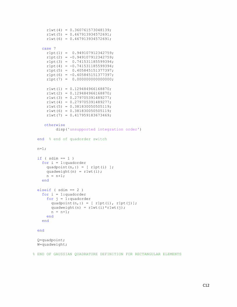
C12

r1wt(4) = 0.360761573048139; r1wt(5) = 0.467913934572691; r1wt(6) = 0.467913934572691;

case 7 r1pt(1) = 0.949107912342759; r1pt(2) = -0.949107912342759; r1pt(3) = 0.741531185599394; r1pt(4) = -0.741531185599394; r1pt(5) = 0.405845151377397; r1pt(6) = -0.405845151377397; r1pt(7) = 0.000000000000000;

r1wt(1) = 0.129484966168870; r1wt(2) = 0.129484966168870; r1wt(3) = 0.279705391489277; r1wt(4) = 0.279705391489277; r1wt(5) = 0.381830050505119; r1wt(6) = 0.381830050505119; r1wt(7) = 0.417959183673469;

otherwise disp('unsupported integration order')

end % end of quadorder switch

n=1;

if ( sdim == 1 ) for i = 1:quadorder quadpoint(n,:) = [ r1pt(i) ]; quadweight(n) = r1wt(i); n = n+1; end

elseif ( sdim == 2 ) for i = 1:quadorder for j = 1:quadorder quadpoint(n,:) = [ r1pt(i), r1pt(j)]; quadweight(n) = r1wt(i)*r1wt(j); n = n+1; end end

end

Q=quadpoint; W=quadweight;

% END OF GAUSSIAN QUADRATURE DEFINITION FOR RECTANGULAR ELEMENTS

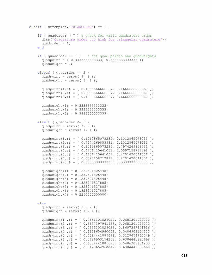
C13

elseif ( strcmp(qt,'TRIANGULAR') == 1 )

if ( quadorder > 7 ) % check for valid quadrature order disp('Quadrature order too high for triangular quadrature'); quadorder = 1; end

if ( quadorder == 1 ) % set quad points and quadweights quadpoint = [ 0.3333333333333, 0.3333333333333 ]; quadweight = 1;

elseif ( quadorder == 2 ) quadpoint = zeros( 3, 2 ); quadweight = zeros( 3, 1 );

quadpoint(1,:) = [ 0.1666666666667, 0.1666666666667 ]; quadpoint(2,:) = [ 0.6666666666667, 0.1666666666667 ]; quadpoint(3,:) = [ 0.1666666666667, 0.6666666666667 ];

quadweight(1) = 0.3333333333333; quadweight(2) = 0.3333333333333; quadweight(3) = 0.3333333333333;

elseif ( quadorder <= 5 ) quadpoint = zeros( 7, 2 ); quadweight = zeros( 7, 1 );

quadpoint(1,:) = [ 0.1012865073235, 0.1012865073235 ]; quadpoint(2,:) = [ 0.7974269853531, 0.1012865073235 ]; quadpoint(3,:) = [ 0.1012865073235, 0.7974269853531 ]; quadpoint(4,:) = [ 0.4701420641051, 0.0597158717898 ]; quadpoint(5,:) = [ 0.4701420641051, 0.4701420641051 ]; quadpoint(6,:) = [ 0.0597158717898, 0.4701420641051 ]; quadpoint(7,:) = [ 0.3333333333333, 0.3333333333333 ];

quadweight(1) = 0.1259391805448; quadweight(2) = 0.1259391805448; quadweight(3) = 0.1259391805448; quadweight(4) = 0.1323941527885; quadweight(5) = 0.1323941527885; quadweight(6) = 0.1323941527885; quadweight(7) = 0.2250000000000;

else quadpoint = zeros( 13, 2 ); quadweight = zeros( 13, 1 );

quadpoint(1 ,:) = [ 0.0651301029022, 0.0651301029022 ]; quadpoint(2 ,:) = [ 0.8697397941956, 0.0651301029022 ]; quadpoint(3 ,:) = [ 0.0651301029022, 0.8697397941956 ]; quadpoint(4 ,:) = [ 0.3128654960049, 0.0486903154253 ]; quadpoint(5 ,:) = [ 0.6384441885698, 0.3128654960049 ]; quadpoint(6 ,:) = [ 0.0486903154253, 0.6384441885698 ]; quadpoint(7 ,:) = [ 0.6384441885698, 0.0486903154253 ]; quadpoint(8 ,:) = [ 0.3128654960049, 0.6384441885698 ];

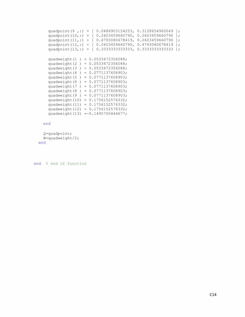
C14

quadpoint(9 ,:) = [ 0.0486903154253, 0.3128654960049 ]; quadpoint(10,:) = [ 0.2603459660790, 0.2603459660790 ]; quadpoint(11,:) = [ 0.4793080678419, 0.2603459660790 ]; quadpoint(12,:) = [ 0.2603459660790, 0.4793080678419 ]; quadpoint(13,:) = [ 0.3333333333333, 0.3333333333333 ];

quadweight(1 ) = 0.0533472356088; quadweight(2 ) = 0.0533472356088; quadweight(3 ) = 0.0533472356088; quadweight(4 ) = 0.0771137608903; quadweight(5 ) = 0.0771137608903; quadweight(6 ) = 0.0771137608903; quadweight(7 ) = 0.0771137608903; quadweight(8 ) = 0.0771137608903; quadweight(9 ) = 0.0771137608903; quadweight(10) = 0.1756152576332; quadweight(11) = 0.1756152576332; quadweight(12) = 0.1756152576332; quadweight(13) =-0.1495700444677;

end

Q=quadpoint; W=quadweight/2; end


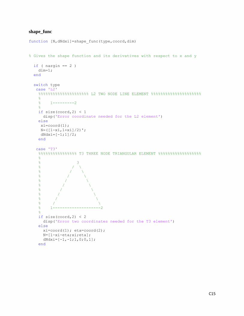
C15

shape_func

function [N,dNdxi]=shape_func(type,coord,dim)

% Gives the shape function and its derivatives with respect to x and y

if ( nargin == 2 ) dim=1; end

switch type case 'L2' %%%%%%%%%%%%%%%%%%%%% L2 TWO NODE LINE ELEMENT %%%%%%%%%%%%%%%%%%%%% % % 1---------2 % if size(coord,2) < 1 disp('Error coordinate needed for the L2 element') else xi=coord(1); N=([1-xi,1+xi]/2)'; dNdxi=[-1;1]/2; end

case 'T3' %%%%%%%%%%%%%%%% T3 THREE NODE TRIANGULAR ELEMENT %%%%%%%%%%%%%%%%%% % % 3 % / \ % / \ % / \ % / \ % / \ % / \ % / \ % / \ % / \ % 1--------------------2 % if size(coord,2) < 2 disp('Error two coordinates needed for the T3 element') else xi=coord(1); eta=coord(2); N=[1-xi-eta;xi;eta]; dNdxi=[-1,-1;1,0;0,1]; end

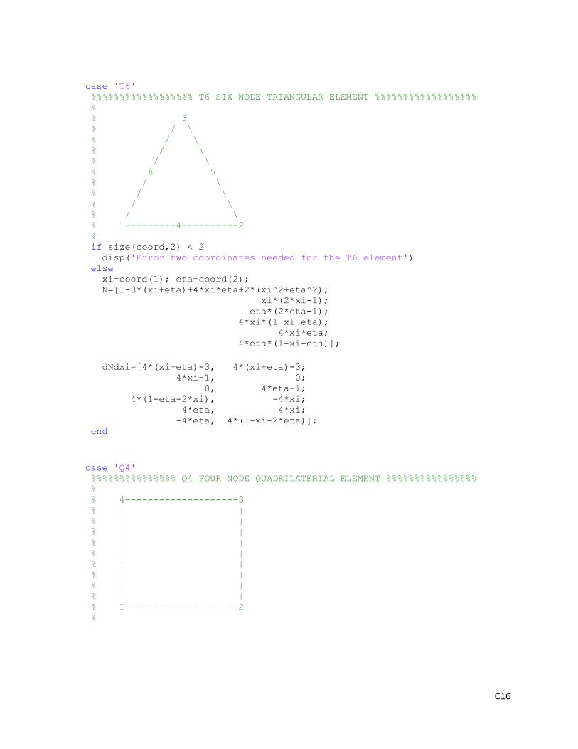
C16

case 'T6' %%%%%%%%%%%%%%%%%% T6 SIX NODE TRIANGULAR ELEMENT %%%%%%%%%%%%%%%%%% % % 3 % / \ % / \ % / \ % / \ % 6 5 % / \ % / \ % / \ % / \ % 1---------4----------2 % if size(coord,2) < 2 disp('Error two coordinates needed for the T6 element') else xi=coord(1); eta=coord(2); N=[1-3*(xi+eta)+4*xi*eta+2*(xi^2+eta^2); xi*(2*xi-1); eta*(2*eta-1); 4*xi*(1-xi-eta); 4*xi*eta; 4*eta*(1-xi-eta)];

dNdxi=[4*(xi+eta)-3, 4*(xi+eta)-3; 4*xi-1, 0; 0, 4*eta-1; 4*(1-eta-2*xi), -4*xi; 4*eta, 4*xi; -4*eta, 4*(1-xi-2*eta)]; end

case 'Q4' %%%%%%%%%%%%%%% Q4 FOUR NODE QUADRILATERIAL ELEMENT %%%%%%%%%%%%%%%% % % 4--------------------3 % | | % | | % | | % | | % | | % | | % | | % | | % | | % 1--------------------2 %

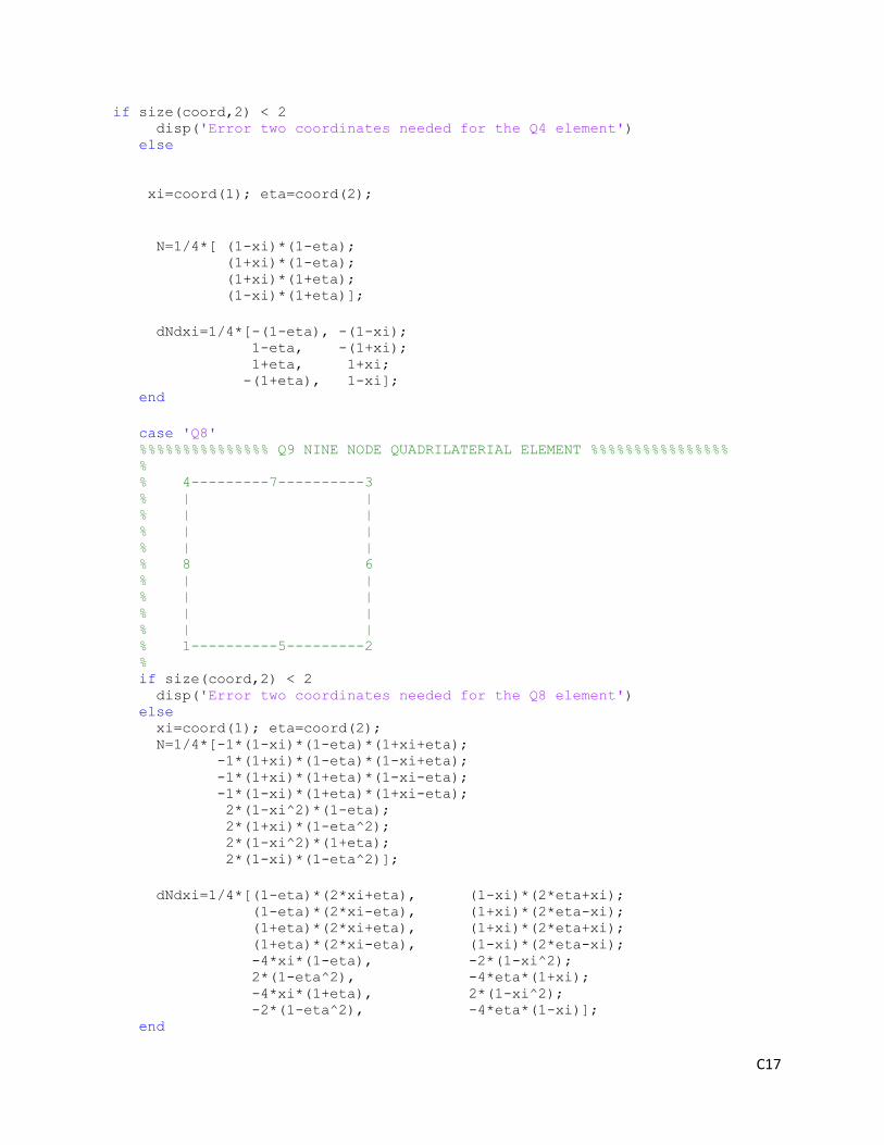
C17

if size(coord,2) < 2 disp('Error two coordinates needed for the Q4 element') else

xi=coord(1); eta=coord(2);

N=1/4*[ (1-xi)*(1-eta); (1+xi)*(1-eta); (1+xi)*(1+eta); (1-xi)*(1+eta)];

dNdxi=1/4*[-(1-eta), -(1-xi); 1-eta, -(1+xi); 1+eta, 1+xi; -(1+eta), 1-xi]; end

case 'Q8' %%%%%%%%%%%%%%% Q9 NINE NODE QUADRILATERIAL ELEMENT %%%%%%%%%%%%%%%% % % 4---------7----------3 % | | % | | % | | % | | % 8 6 % | | % | | % | | % | | % 1----------5---------2 % if size(coord,2) < 2 disp('Error two coordinates needed for the Q8 element') else xi=coord(1); eta=coord(2); N=1/4*[-1*(1-xi)*(1-eta)*(1+xi+eta); -1*(1+xi)*(1-eta)*(1-xi+eta); -1*(1+xi)*(1+eta)*(1-xi-eta); -1*(1-xi)*(1+eta)*(1+xi-eta); 2*(1-xi^2)*(1-eta); 2*(1+xi)*(1-eta^2); 2*(1-xi^2)*(1+eta); 2*(1-xi)*(1-eta^2)];

dNdxi=1/4*[(1-eta)*(2*xi+eta), (1-xi)*(2*eta+xi); (1-eta)*(2*xi-eta), (1+xi)*(2*eta-xi); (1+eta)*(2*xi+eta), (1+xi)*(2*eta+xi); (1+eta)*(2*xi-eta), (1-xi)*(2*eta-xi); -4*xi*(1-eta), -2*(1-xi^2); 2*(1-eta^2), -4*eta*(1+xi); -4*xi*(1+eta), 2*(1-xi^2); -2*(1-eta^2), -4*eta*(1-xi)]; end

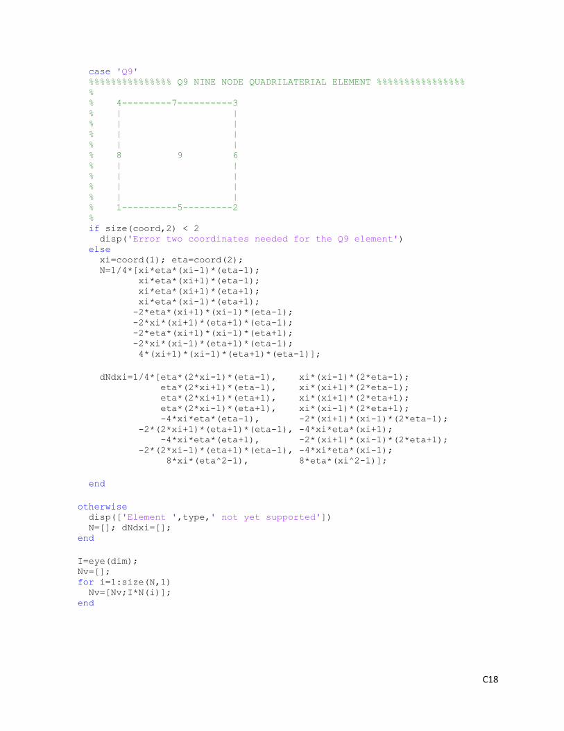
C18

case 'Q9' %%%%%%%%%%%%%%% Q9 NINE NODE QUADRILATERIAL ELEMENT %%%%%%%%%%%%%%%% % % 4---------7----------3 % | | % | | % | | % | | % 8 9 6 % | | % | | % | | % | | % 1----------5---------2 % if size(coord,2) < 2 disp('Error two coordinates needed for the Q9 element') else xi=coord(1); eta=coord(2); N=1/4*[xi*eta*(xi-1)*(eta-1); xi*eta*(xi+1)*(eta-1); xi*eta*(xi+1)*(eta+1); xi*eta*(xi-1)*(eta+1); -2*eta*(xi+1)*(xi-1)*(eta-1); -2*xi*(xi+1)*(eta+1)*(eta-1); -2*eta*(xi+1)*(xi-1)*(eta+1); -2*xi*(xi-1)*(eta+1)*(eta-1); 4*(xi+1)*(xi-1)*(eta+1)*(eta-1)];

dNdxi=1/4*[eta*(2*xi-1)*(eta-1), xi*(xi-1)*(2*eta-1); eta*(2*xi+1)*(eta-1), xi*(xi+1)*(2*eta-1); eta*(2*xi+1)*(eta+1), xi*(xi+1)*(2*eta+1); eta*(2*xi-1)*(eta+1), xi*(xi-1)*(2*eta+1); -4*xi*eta*(eta-1), -2*(xi+1)*(xi-1)*(2*eta-1); -2*(2*xi+1)*(eta+1)*(eta-1), -4*xi*eta*(xi+1); -4*xi*eta*(eta+1), -2*(xi+1)*(xi-1)*(2*eta+1); -2*(2*xi-1)*(eta+1)*(eta-1), -4*xi*eta*(xi-1); 8*xi*(eta^2-1), 8*eta*(xi^2-1)];

end

otherwise disp(['Element ',type,' not yet supported']) N=[]; dNdxi=[]; end

I=eye(dim); Nv=[]; for i=1:size(N,1) Nv=[Nv;I*N(i)]; end

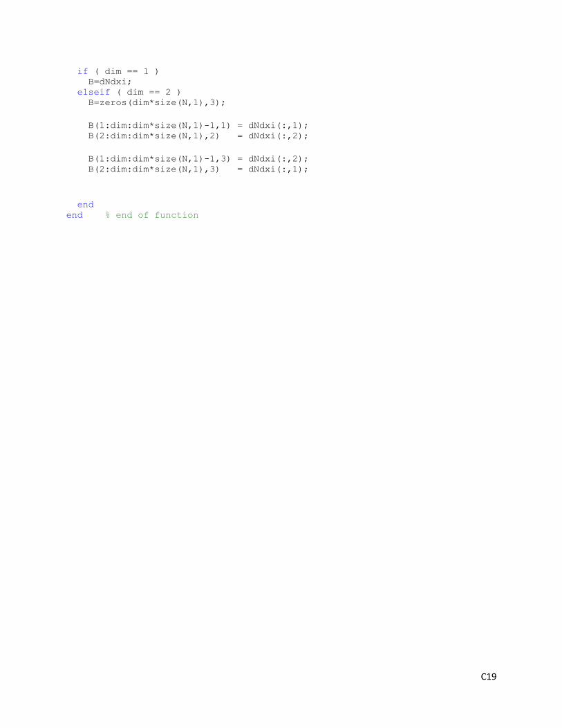
C19

if ( dim == 1 ) B=dNdxi; elseif ( dim == 2 ) B=zeros(dim*size(N,1),3);

B(1:dim:dim*size(N,1)-1,1) = dNdxi(:,1); B(2:dim:dim*size(N,1),2) = dNdxi(:,2);

B(1:dim:dim*size(N,1)-1,3) = dNdxi(:,2); B(2:dim:dim*size(N,1),3) = dNdxi(:,1);

end end % end of function

C20

displacements

function [U,u_x,u_y] =displacements(dispNodes,dispNodes1,numnode,K,f,selfwt)

% evaluates the unknown degree of freedom (displacements) at the nodes

total_unknown=2*numnode; udofs = [(dispNodes.*2)-1;(dispNodes1.*2)-1]; %prescribed disp.in x-dir vdofs = dispNodes.*2; %prescribed disp. in y-dir dofs=union(udofs(:),vdofs(:)); %overall prescribed disp. unknowndof=setdiff((1:total_unknown)',dofs);

F=f(unknowndof)+selfwt(unknowndof); u=K(unknowndof,unknowndof)\F; U=zeros(total_unknown,1); U(unknowndof)=u; u_x = U(1:2:2*numnode-1) ; % 1 3 5 7 ... u_y = U(2:2:2*numnode) ; % 2 4 6 8 ...


force_matrix

function f=force_matrix(node,topEdge,sigmatoy,sigmatox,load_edge1,load_edge2)

% Generates the force matrix due to externally applied loads % for Q4 and T3 elements.

numnode = size(node,1); total_unknown = numnode*2; f = zeros(total_unknown,1); [W,Q]=gauss_pt_wt(1,'GAUSS',1);

ii1=intersect(find(node(:,1)==load_edge1),unique(topEdge)); jj1=intersect(find(node(:,1)==load_edge2),unique(topEdge)); ii2=find(topEdge(:,1)==ii1); jj2=find(topEdge(:,2)==jj1);

for e =ii2:jj2 sctr = topEdge(e,:); sctry = sctr.*2 ; sctrx = sctr.*2-1; for q=1:size(W,1) pt = Q(q,:); wt = W(q); N = shape_func('L2',pt); J0 = abs( node(sctr(2))-node(sctr(1)) )/2; f(sctry) = f(sctry) + N*sigmatoy*det(J0)*wt; f(sctrx) = f(sctrx) + N*sigmatox*det(J0)*wt; end % end of quadrature loop end % end of element loop


C21

elementdof

function eldof =elementdof(elemType,sctr)

% forms the global degree of freedom nodes in each element from the node % identification number.

switch (elemType) case 'Q9' eldof=[sctr(1)*2-1;sctr(1)*2;... sctr(2)*2-1;sctr(2)*2;... sctr(3)*2-1;sctr(3)*2;... sctr(4)*2-1;sctr(4)*2;... sctr(5)*2-1;sctr(5)*2;... sctr(6)*2-1;sctr(6)*2;... sctr(7)*2-1;sctr(7)*2;... sctr(8)*2-1;sctr(8)*2;... sctr(9)*2-1;sctr(9)*2]; case 'Q8' eldof=[sctr(1)*2-1;sctr(1)*2;... sctr(2)*2-1;sctr(2)*2;... sctr(3)*2-1;sctr(3)*2;... sctr(4)*2-1;sctr(4)*2;... sctr(5)*2-1;sctr(5)*2;... sctr(6)*2-1;sctr(6)*2;... sctr(7)*2-1;sctr(7)*2;... sctr(8)*2-1;sctr(8)*2]; case 'Q4' eldof=[sctr(1)*2-1;sctr(1)*2;... sctr(2)*2-1;sctr(2)*2;... sctr(3)*2-1;sctr(3)*2;... sctr(4)*2-1;sctr(4)*2]; case 'T6' eldof=[sctr(1)*2-1;sctr(1)*2;... sctr(2)*2-1;sctr(2)*2;... sctr(3)*2-1;sctr(3)*2;... sctr(4)*2-1;sctr(4)*2;... sctr(5)*2-1;sctr(5)*2;... sctr(6)*2-1;sctr(6)*2]; case 'T3' eldof=[sctr(1)*2-1;sctr(1)*2;... sctr(2)*2-1;sctr(2)*2;... sctr(3)*2-1;sctr(3)*2]; case 'L3' eldof=[sctr(1)*2-1;sctr(1)*2;... sctr(2)*2-1;sctr(2)*2;... sctr(3)*2-1;sctr(3)*2]; case 'L2' eldof=[sctr(1)*2-1;sctr(1)*2;... sctr(2)*2-1;sctr(2)*2];

end


C22

force_matrix689

function f=force_matrix689(node,topEdge,topEdge1,sigmatoy,sigmatox,...

load_edge1,load_edge2)

% Generates the force matrix due to externally applied loads % for Q9,Q8 and T6 elements.

numnode = size(node,1); total_unknown = numnode*2; f = zeros(total_unknown,1);

[W,Q]=gauss_pt_wt(2,'GAUSS',1);

ii1=intersect(find(node(:,1)==load_edge1),unique(topEdge)); jj1=intersect(find(node(:,1)==load_edge2),unique(topEdge)); ii2=find(topEdge(:,1)==ii1); jj2=find(topEdge(:,2)==jj1); ee2=topEdge1(1:end,2).*2;ee4=ee2-1; ee1=unique(topEdge); ee3=ee1(1:2:end).*2;ee6=ee3-1;

for e =ii2:jj2 sctr = topEdge(e,:); sctry = sctr.*2 ; sctrx = sctr.*2-1;

for q=1:size(W,1) pt = Q(q,:); wt = W(q); [N,dNdxi] = shape_func('L2',pt); J0 = abs( node(sctr(2))-node(sctr(1)) )/2; f(sctry) = f(sctry) + N*sigmatoy*det(J0)*wt; f(sctrx) = f(sctrx) + N*sigmatox*det(J0)*wt; end % of quadrature loop

end % of element loop

f(ee3)=f(ee3)*(2/3); f(ee2)=f(ee2)*(4/3); f(ee6)=f(ee6)*(2/3); f(ee4)=f(ee4)*(4/3);


C23

formdg

function [dg1,dg2,dg3] =formdg(tsi,q,theta)

% calculates the partial derivatives of the plastic potential with respect % to p, J2 and J3.

dg1=sind(tsi); if sind(theta)>0.49 % close to theta=30 corner,smoothen the curve with sw=1; % triaxial compression case s1 > s2 = s3 dg2=(0.25/q)*(3-sw*sind(tsi)); dg3=0;

elseif -1*sind(theta)>049 % close to theta=-30 corner,smoothen the curve sw=-1; % with triaxial extension case s1 = s2 > s3 dg2=(0.25/q)*(3-sw*sind(tsi)); dg3=0; else % all other cases dg2=(sqrt(3)*cosd(theta)/(2*q))*(1+(tand(theta)*tand(3*theta))+... ((sind(tsi)/sqrt(3))*(tand(3*theta)-tand(theta))));

dg3=1.5*((sqrt(3)*sind(theta))+(sind(tsi)*cosd(theta))/(q^2*cosd(3*theta)));


formm

function [m1,m2,m3] = formm(kk,iel,stress)

%Generates the partial derivatives of the p, J2 and J3 with respect to %stress for use in the plastic potential derivative.

s_xx=stress(1,kk,iel);s_yy=stress(2,kk,iel); t_xy=stress(3,kk,iel);s_zz=stress(4,kk,iel); p1=(s_xx+s_yy+s_zz)/3;

sx=s_xx-p1; sy=s_yy-p1; sz=s_zz-p1;

m1=1/(3*(s_xx+s_yy+s_zz))*[1 1 0 1;1 1 0 1;0 0 0 0;1 1 0 1];

m2=1/3*[2 -1 0 -1;-1 2 0 -1;0 0 6 0;-1 -1 0 2];

m3=1/3*[sx sz t_xy sz;sz sy t_xy sx;t_xy t_xy -3*sz -2*t_xy;sz sx -2*t_xy

sz];

end % emd of function

C24

internalrxn

function [r] = internalrxn( node,element,elemType,normal_order,stress)

%Generates the vector of nodal force reactions due to internal stress. it %can be used out side the iteration loop if the stresses at each gauss %point is given.

numnode = size(node,1); numelem = size(element,1); total_unknown = numnode*2; r=zeros(total_unknown,1);

for iel = 1 : numelem sctr = element(iel,:); % element connectivity nn = length(sctr); % number of nodes per element eldof =elementdof(elemType,sctr); %element degree of freedom [W,Q] = gauss_rule(iel,elemType,normal_order); % determine GP

for kk = 1 :nn pt =Q(kk,:); [N,dNdxi] = shape_func(elemType,pt); J0 = node(sctr,:)'*dNdxi; Bfem4 =Bmatrix4(pt,elemType,iel); r(eldof) =r(eldof)+Bfem4'*stress(:,kk,iel)*W(kk)*det(J0); end % end of looping on Gauss Points end % end of looping on elements end % end of function

invariants

function [p,q,theta] = invariants( stress )

%calculates the stress invariants for a single gauss point

s_xx=stress(1); s_yy=stress(2); p=(s_xx+s_yy+s_zz)/3; t_xy=stress(3); s_zz=stress(4); t=sqrt((s_xx-s_yy)^2+(s_yy-s_zz)^2+(s_zz-s_xx)^2+6*t_xy^2)/sqrt(3); q=sqrt(1.5)*t; sx=s_xx-p; sy=s_yy-p; sz=s_zz-p; if q<1e-6 theta=0; else j3=sx*sy*sz-(sx*t_xy^2); sine=-3*j3*sqrt(6)/t^3; if sine>1; sine=1; end if sine<-1; sine=-1; end theta=1/3*(asind(sine)); end


C25

invariants1

function [p,q,theta] =invariants1(element,stress)

% calculates the stress invariants at each gauss point.This can be used % outside the iteration loop.

numelem=size(element,1); nonelm=size(element,2); p=zeros(1,nonelm,numelem); q=zeros(1,nonelm,numelem); theta=zeros(1,nonelm,numelem);

for iel = 1 : numelem sctr = element(iel,:); % element connectivity nn = length(sctr); % number of nodes per element

for kk = 1:nn s_xx=stress(1,kk,iel);s_yy=stress(2,kk,iel); t_xy=stress(3,kk,iel);s_zz=stress(4,kk,iel); p1=(s_xx+s_yy+s_zz)/3; t=sqrt((s_xx-s_yy)^2+(s_yy-s_zz)^2+(s_zz-s_xx)^2+6*t_xy^2)/sqrt(3); q1=sqrt(1.5)*t; sx=s_xx-p1; sy=s_yy-p1; sz=s_zz-p1; if q1<1e-6 theta11=0; else j3=sx*sy*sz-(sx*t_xy^2); sine=-3*j3*sqrt(6)/t^3; if sine>1; sine=1; end if sine<-1; sine=-1; end theta11=1/3*(asind(sine)); end p(:,kk,iel)=p1; q(:,kk,iel)=q1; theta(:,kk,iel)=theta11; end % end of looping on GPs end % end of looping on elements


C26

invariants2

function [p,q,theta] =invariants2(kk,iel,stress)

% calculates the stress invariants at each gauss point.This can be used % inside the iteration loop.

s_xx=stress(1,kk,iel);s_yy=stress(2,kk,iel); t_xy=stress(3,kk,iel);s_zz=stress(4,kk,iel); p=(s_xx+s_yy+s_zz)/3; t=sqrt((s_xx-s_yy)^2+(s_yy-s_zz)^2+(s_zz-s_xx)^2+6*t_xy^2)/sqrt(3); q=sqrt(1.5)*t; sx=s_xx-p; sy=s_yy-p; sz=s_zz-p; if q<1e-6 theta=0; else j3=sx*sy*sz-(sx*t_xy^2); sine=-3*j3*sqrt(6)/t^3; if sine>1; sine=1; end if sine<-1; sine=-1; end theta=1/3*(asind(sine)); end


makedfds

function [dfds] =makedfds(phi,element,iel,kk,stress)

%Forms the partial derivatives of the yield function with %respect to stress at each gauss point.

numelem=size(element,1); nonelm=size(element,2); dfds=zeros(4,nonelm,numelem);


t=sqrt((s_xx-s_yy)^2+(s_yy-s_zz)^2+(s_zz-s_xx)^2+6*t_xy^2)/sqrt(3); q1=sqrt(1.5)*t; sx=s_xx-p1; sy=s_yy-p1; sz=s_zz-p1; j2=-sx*sy-sy*sz-sz*sx+t_xy^2; j3=sx*sy*sz-(sx*t_xy^2); th=-3*sqrt(3)*j3/(2*j2^1.5);

C27

if th>1 th=1; end if th<-1 th=-1; end theta1=asind(th)/3;

if sind(theta1)>0.49 % close to theta=30 corner,smoothen the curve % with triaxial compression case s1 > s2 = s3 sw=-1; cphi=0.25*sqrt(3/j2)*(1+(sw*sind(phi)/3));

dfds(:,kk,iel)=[(sind(phi)/3)+sx*cphi;... (sind(phi)/3)+sy*cphi;... t_xy*cphi;... (sind(phi)/3)+sz*cphi];

elseif (-1*sind(theta1))>0.49 % close to theta=-30 corner,smoothen the curve % curve with triaxial extension case s1 = s2 > s3 sw=1; cphi=0.25*sqrt(3/j2)*(1+(sw*sind(phi)/3));

dfds(:,kk,iel)=[(sind(phi)/3)+sx*cphi;... (sind(phi)/3)+sy*cphi;... t_xy*cphi;... (sind(phi)/3)+sz*cphi]; else alpha=atand(abs((s_xx-s_yy)/(2*t_xy))); % all other conditions k1=1;k2=1; if abs(s_xx)>abs(s_yy) k1=-1; end if t_xy <0 k2=-1; end

dfds(:,kk,iel)=[sind(phi)+k1*sind(alpha);... sind(phi)-k1*sind(alpha);... 2*k2*cosd(alpha);... 0]; end


C28

makedgds function [dgds] =makedgds(tsi,element,iel,kk,stress)

%Forms the partial derivatives of the plastic potential function with %respect to stress at each gauss point.

numelem=size(element,1); nonelm=size(element,2); dgds=zeros(4,nonelm,numelem);


t=sqrt((s_xx-s_yy)^2+(s_yy-s_zz)^2+(s_zz-s_xx)^2+6*t_xy^2)/sqrt(3); q1=sqrt(1.5)*t; sx=s_xx-p1; sy=s_yy-p1; sz=s_zz-p1; j2=-sx*sy-sy*sz-sz*sx+t_xy^2; j3=sx*sy*sz-(sx*t_xy^2); th=-3*sqrt(3)*j3/(2*j2^1.5);

if th>1 th=1; end if th<-1 th=-1; end theta1=asind(th)/3;

if sind(theta1)>0.49 % close to theta=30 corner,smoothen the curve % with triaxial compression case s1 > s2 = s3 sw=-1; ctsi=0.25*sqrt(3/j2)*(1+(sw*sind(tsi)/3));

dgds(:,kk,iel)=[(sind(tsi)/3)+sx*ctsi;... (sind(tsi)/3)+sy*ctsi;... t_xy*ctsi;... (sind(tsi)/3)+sz*ctsi];

elseif (-1*sind(theta1))>0.49 % close to theta=-30 corner,smoothen the curve % curve with triaxial extension case s1 = s2 > s3 sw=1; ctsi=0.25*sqrt(3/j2)*(1+(sw*sind(tsi)/3));

dgds(:,kk,iel)=[(sind(tsi)/3)+sx*ctsi;... (sind(tsi)/3)+sy*ctsi;... t_xy*ctsi;... (sind(tsi)/3)+sz*ctsi]; else

C29

alpha=atand(abs((s_xx-s_yy)/(2*t_xy))); % all other conditions k1=1;k2=1; if abs(s_xx)>abs(s_yy) k1=-1; end if t_xy <0 k2=-1; end

dgds(:,kk,iel)=[sind(tsi)+k1*sind(alpha);... sind(tsi)-k1*sind(alpha);... 2*k2*cosd(alpha);... 0]; end


plastic_mat

function [CP] = plastic_mat(E,nu,phi,tsi,iel,kk,stress)

% Generates the plastic constitutive matix CP at each gauss point


t=sqrt((s_xx-s_yy)^2+(s_yy-s_zz)^2+(s_zz-s_xx)^2+6*t_xy^2)/sqrt(3); q=sqrt(1.5)*t; sx=s_xx-p1; sy=s_yy-p1; sz=s_zz-p1; j2=-sx*sy-sy*sz-sz*sx+t_xy^2; j3=sx*sy*sz-(sx*t_xy^2); th=-3*sqrt(3)*j3/(2*j2^1.5); if th>1 th=1; end if th<-1 th=-1; end theta1=asind(th)/3;

if sind(theta1)>0.495 % close to theta=30 corner,smoothen the curve % with triaxial compression case s1 > s2 = s3 sw=-1; cphi=0.25*sqrt(3/j2)*(1+(sw*sind(phi)/3)); ctsi=0.25*sqrt(3/j2)*(1+(sw*sind(tsi)/3)); kphi=sind(phi)*(1+nu)/3; ktsi=sind(tsi)*(1+nu)/3; c1=kphi+cphi*(sx*(1-nu)+nu*(sy+sz)); c2=kphi+cphi*(sy*(1-nu)+nu*(sx+sz)); c3=cphi*(1-2*nu)*t_xy; c4=kphi+cphi*(sz*(1-nu)+nu*(sx+sy));

C30

r1=ktsi+ctsi*(sx*(1-nu)+nu*(sy+sz)); r2=ktsi+ctsi*(sy*(1-nu)+nu*(sx+sz)); r3=ctsi*(1-2*nu)*t_xy; r4=ktsi+ctsi*(sz*(1-nu)+nu*(sx+sy)); A=[r1*c1 r1*c2 r1*c3 r1*c4;... r2*c1 r2*c2 r2*c3 r2*c4;... r3*c1 r3*c2 r3*c3 r3*c4;... r4*c1 r4*c2 r4*c3 r4*c4]; CP=E*A/((1+nu)*(1-2*nu)*(kphi*sind(tsi)+2*cphi*ctsi*j2*(1-2*nu)));

elseif -1*sind(theta1)> 0.49 sw=1; % close to theta=-30 corner,smoothen the curve % with triaxial extension case s1 = s2 > s3 cphi=0.25*sqrt(3/j2)*(1+(sw*sind(phi)/3)); ctsi=0.25*sqrt(3/j2)*(1+(sw*sind(tsi)/3)); kphi=sind(phi)*(1+nu)/3; ktsi=sind(tsi)*(1+nu)/3; c1=kphi+cphi*(sx*(1-nu)+nu*(sy+sz)); c2=kphi+cphi*(sy*(1-nu)+nu*(sx+sz)); c3=cphi*(1-2*nu)*t_xy; c4=kphi+cphi*(sz*(1-nu)+nu*(sx+sy)); r1=ktsi+ctsi*(sx*(1-nu)+nu*(sy+sz)); r2=ktsi+ctsi*(sy*(1-nu)+nu*(sx+sz)); r3=ctsi*(1-2*nu)*t_xy; r4=ktsi+ctsi*(sz*(1-nu)+nu*(sx+sy)); A=[r1*c1 r1*c2 r1*c3 r1*c4;... r2*c1 r2*c2 r2*c3 r2*c4;... r3*c1 r3*c2 r3*c3 r3*c4;... r4*c1 r4*c2 r4*c3 r4*c4]; CP=E*A/((1+nu)*(1-2*nu)*(kphi*sind(tsi)+2*cphi*ctsi*j2*(1-2*nu)));

else % all other cases alpha=atand(abs((s_xx-s_yy)/(2*t_xy))); k1=1;k2=1; if abs(s_xx)>abs(s_yy) k1=-1; end if t_xy <0 k2=-1; end c1=sind(phi)+k1*(1-2*nu)*sind(alpha); c2=sind(phi)-k1*(1-2*nu)*sind(alpha); c3=k2*(1-2*nu)*cosd(alpha); c4=2*nu*sind(phi); r1=sind(tsi)+k1*(1-2*nu)*sind(alpha); r2=sind(tsi)-k1*(1-2*nu)*sind(alpha); r3=k2*(1-2*nu)*cosd(alpha); r4=2*nu*sind(tsi); A=[r1*c1 r1*c2 r1*c3 r1*c4;... r2*c1 r2*c2 r2*c3 r2*c4;... r3*c1 r3*c2 r3*c3 r3*c4;... r4*c1 r4*c2 r4*c3 r4*c4]; CP=E*A/(2*(1+nu)*(1-2*nu)*(1-2*nu+sind(phi)*sind(tsi)));


C31

principal_stress

function [s1,s2,s3] = principal_stress(kk,iel,p,q,theta)

%calcualtes the principal stresses from the stress invariants

s1=p(:,kk,iel)+q(:,kk,iel)*(2/3)*sind(theta(:,kk,iel)-120);

s2=p(:,kk,iel)+q(:,kk,iel)*(2/3)*sind(theta(:,kk,iel));

s3=p(:,kk,iel)+q(:,kk,iel)*(2/3)*sind(theta(:,kk,iel)+120);


selfwt_matrix function selfwt=selfwt_matrix(elemType,normal_order,gamma,node,element)

% Generates the force matrix due to self weight

numelem=size(element,1); numnode = size(node,1); total_unknown = numnode*2; selfwt=zeros(total_unknown,1);

for iel = 1 : numelem sctr1 = element(iel,:); % element connectivity swpt=sctr1.*2; %element degree of freedom

[W,Q] = gauss_rule(iel,elemType,normal_order);

for q=1:size(W,1) pt = Q(q,:); wt = W(q); % quadrature point [N,dNdxi]=shape_func(elemType,pt); J0 = node(sctr1,:)'*dNdxi; % element Jacobian matrix selfwt(swpt) = selfwt(swpt)+ N*(-1*gamma)*det(J0)*wt; end end end % end of function

C32

stiffness_matrix function K=stiffness_matrix(node,element,elemType,normal_order,C)

% Generates the element and global stiffness matrix

numnode = size(node,1); numelem = size(element,1); total_unknown = numnode*2; K = zeros(total_unknown,total_unknown);

for iel = 1 : numelem sctr = element(iel,:); % element connectivity nn = length(sctr); % number of nodes per element eldof =elementdof(elemType,sctr); %element degree of freedom

[W,Q] = gauss_rule(iel,elemType,normal_order);

for kk = 1 : size(W,1) % Loop on Gauss points pt = Q(kk,:); % quadrature point [N,dNdxi] = shape_func(elemType,pt); J0 = node(sctr,:)'*dNdxi; % element Jacobian matrix Bfem =Bmatrix(pt,elemType,iel); K(eldof,eldof) = K(eldof,eldof)+Bfem'*C(1:3,1:3)*Bfem*W(kk)*det(J0); end % end of looping on Gauss Points end % end of looping on elements end % end of function

stress_calculation

function [stress,strain] =stress_calculation(node,element,elemType,...

U,normal_order,C)

% calculates the element strains and stresses at the nodes % in x, y and xy directions.

numelem=size(element,1);

switch elemType case 'Q9' stresspoints=[-1 -1;1 -1;1 1;-1 1;0 -1;1 0;0 1;-1 0;0 0]; case 'Q8' stresspoints=[-1 -1;1 -1;1 1;-1 1;0 -1;1 0;0 1;-1 0]; case 'Q4' stresspoints=[-1 -1;1 -1;1 1;-1 1]; case 'T3' stresspoints=[0 0;1 0;0 1]; otherwise stresspoints=[0 0;1 0;0 1;0.5 0;0.5 0.5;0 0.5]; end

for iel = 1 : numelem sctr = element(iel,:); % element connectivity nn = length(sctr); % number of nodes per element

C33

eldof =elementdof(elemType,sctr); [W,Q] = gauss_rule(iel,elemType,normal_order);

for kk = 1:nn pt = stresspoints(kk,:); % quadrature point [N,dNdxi] = shape_func(elemType,pt); % element shape functions J0 = node(sctr,:)'*dNdxi; % element Jacobian matrix Bfem =Bmatrix(pt,elemType,iel); strain=Bfem*U(eldof); stress(iel,kk,:)=C*strain;

end % end of looping on gauss points

end % end of looping on elements


Supportcond function [topEdge,topEdge1,dispNodes,dispNodes1]= ...

supportcond(elemType,numx,numy)

% Forms a vector of nodes which are restrained in x direction or in both % x and y direction which are the supports of the domain. %It also forms a matrix of nodes for load application at the top of the

%domain.

switch elemType case 'Q9' nnx=numx*2+1; nny=numy*2+1; urn =nnx*nny; % upper right node number uln =urn-(nnx-1); % upper left node number lrn = nnx; % lower right node number lln = 1; % lower left node number

topEdge = [ uln:1:(urn-1); (uln+1):1:urn ]'; topEdge1=[uln:2:(urn-2); (uln+1):2:(urn-1);(uln+2):2:urn ]'; botEdge = [ lln:1:(lrn-1); (lln+1):1:lrn ]'; leftEdge=[(lln:nnx:(uln-nnx));(lln+nnx:nnx:uln)]'; rightEdge=[(nnx:nnx:(urn-nnx));(nnx+nnx:nnx:urn)]'; % GET NODES ON ESSENTIAL BOUNDARY

botNodes = unique(botEdge); topNodes = unique(topEdge); leftNodes = unique(leftEdge); rightNodes = unique(rightEdge); dispNodes = botNodes; rightNodes1=rightNodes(2:end); leftNodes1=leftNodes(2:end); dispNodes1=union(leftNodes1,rightNodes1);

C34

case 'Q8' nnx=numx*2+1; nny=numy*2+1; urn =(nnx*nny)-(numx*numy);% upper right node number uln =urn-(nnx-1); % upper left node number lrn = nnx; % lower right node number lln = 1; % lower left node number

topEdge = [ uln:1:(urn-1); (uln+1):1:urn ]'; topEdge1=[uln:2:(urn-2); (uln+1):2:(urn-1);(uln+2):2:urn ]'; botEdge = [ lln:1:(lrn-1); (lln+1):1:lrn ]'; % GET NODES ON ESSENTIAL BOUNDARY botNodes = unique(botEdge); topNodes = unique(topEdge); leftNodes = union((lln:nnx+numx+1:uln),...

(nnx+1:nnx+numx+1:uln-numx+1))'; rightNodes = union((nnx:nnx+numx+1:urn),...

(nnx+numx+1:nnx+numx+1:urn-nnx))'; dispNodes = botNodes; rightNodes1=rightNodes(2:end); leftNodes1=leftNodes(2:end); dispNodes1=union(leftNodes1,rightNodes1); leftEdge=[leftNodes(1:nny-1,:),leftNodes1]; rightEdge=[rightNodes(1:nny-1,:),rightNodes1]; case {'Q4','T3'} nnx=numx+1; nny=numy+1; uln = nnx*(nny-1)+1; % upper left node number urn = nnx*nny; % upper right node number lrn = nnx; % lower right node number lln = 1; % lower left node number topEdge = [ uln:1:(urn-1); (uln+1):1:urn ]'; topEdge1=topEdge; botEdge = [ lln:1:(lrn-1); (lln+1):1:lrn ]'; rightEdge = (lrn:nnx:(urn))'; % GET NODES ON ESSENTIAL BOUNDARY

botNodes = unique(botEdge); topNodes = unique(topEdge); rightNodes = unique(rightEdge); leftNodes = rightNodes-(nnx-1); dispNodes = botNodes; rightNodes1=rightNodes(2:end); leftNodes1=leftNodes(2:end); dispNodes1=union(leftNodes1,rightNodes1); case 'T6' nnx=numx*2+1; nny=numy*2+1; urn =nnx*nny; % upper right node number uln =urn-(nnx-1); % upper left node number lrn = nnx; % lower right node number lln = 1; % lower left node number

topEdge = [ uln:1:(urn-1); (uln+1):1:urn ]'; topEdge1=[uln:2:(urn-2); (uln+1):2:(urn-1);(uln+2):2:urn ]'; botEdge = [ lln:1:(lrn-1); (lln+1):1:lrn ]';

C35

% GET NODES ON ESSENTIAL BOUNDARY botNodes = unique(botEdge); topNodes = unique(topEdge); leftNodes =(lln:nnx:uln)'; rightNodes =(lrn:nnx:urn)'; dispNodes = botNodes; rightNodes1=rightNodes(2:end); leftNodes1=leftNodes(2:end); dispNodes1=union(leftNodes1,rightNodes1); leftEdge=[leftNodes(1:nny-1,:),leftNodes1]; rightEdge=[rightNodes(1:nny-1,:),rightNodes1]; end end % end of function

plot_def

function plot_def(fac,u_x,u_y,elemType,dispNodes,dispNodes1)

% Plots the deformed finite element mesh with the support condition

global node element

figure clf hold on plot_mesh(node+fac*[u_x u_y],element,elemType,'b-'); title(' Numerical deformed mesh ') plot(node(dispNodes,1),node(dispNodes,2),'ks'); plot(node(dispNodes1,1),node(dispNodes1,2),'ko');


plot_defo

function plot_defo(fac,u_x,u_y,elemType)

% plots the color coded displacement intensity in the finite element % region along with color bar scale.

global node element

figure clf subplot(2,1,1); plot_field(node+fac*[u_x u_y],element,elemType,u_x); colorbar title('Deformation plot, U_X')

subplot(2,1,2); plot_field(node+fac*[u_x u_y],element,elemType,u_y); colorbar title('Deformation plot, U_Y')


C36

plot_field function plot_field(node,connect,elem_type,field)

% Forms a color dependent finite element mesh for plotting outputs

if ( size(field) == size(connect) ) elementalField=1; else elementalField=0; end % fill node if needed if (size(node,2) < 3) for c=size(node,2)+1:3 node(:,c)=[zeros(size(node,1),1)]; end end

holdState=ishold; hold on

if ( strcmp(elem_type,'Q9') ) % Q9 element ord=[1,5,2,6,3,7,4,8,1]; elseif ( strcmp(elem_type,'T3') ) % T3 element ord=[1,2,3,1]; elseif ( strcmp(elem_type,'T6') ) % T6 element ord=[1,4,2,5,3,6,1]; elseif ( strcmp(elem_type,'Q4') ) % Q4 element ord=[1,2,3,4,1]; elseif ( strcmp(elem_type,'Q8') ) % Q8 element ord=[1,5,2,6,3,7,4,8,1]; elseif ( strcmp(elem_type,'L2') ) % L2 element ord=[1,2]; end

for e=1:size(connect,1) xpt=node(connect(e,ord),1); ypt=node(connect(e,ord),2); zpt=node(connect(e,ord),3);

if ( elementalField ) fpt=field(e,ord); else fpt=field(connect(e,ord)); end

fill3(xpt,ypt,zpt,fpt) end

shading interp axis equal if ( ~holdState ) hold off end end % end of fuction

C37

plot_m

function plot_m(elemType,dispNodes,dispNodes1)

% Plots the finite element mesh with the support condition

global node element

v=get(0,'ScreenSize'); figure('Color',[1 1 1]) hold on plot_mesh(node,element,elemType,'b-'); plot(node(dispNodes,1),node(dispNodes,2),'ks'); plot(node(dispNodes1,1),node(dispNodes1,2),'ko'); axis off


plot_sig function plot_sig(fac,u_x,u_y,elemType,stress)

% plots the color coded stress distribution in the finite element % region along with color bar scale.

global node element figure clf subplot(3,1,1); plot_field(node+fac*[u_x u_y],element,elemType,stress(:,:,1)); colorbar title('Stress plot, sigma_xx')

subplot(3,1,2); plot_field(node+fac*[u_x u_y],element,elemType,stress(:,:,2)); colorbar title('Stress plot, sigma_yy')

subplot(3,1,3); plot_field(node+fac*[u_x u_y],element,elemType,stress(:,:,3)); colorbar title('Stress plot, sigma_xy')


C38

plot_mesh function plot_mesh(node,connect,elem_type,se)

% Plots the finite element mesh

if ( nargin < 4 ) se='w-'; end

holdState=ishold; hold on

% fill node if needed if (size(node,2) < 3) for c=size(node,2)+1:3 node(:,c)=[zeros(size(node,1),1)]; end end

for e=1:size(connect,1)

if ( strcmp(elem_type,'Q9') ) % 9-node quad element ord=[1,5,2,6,3,7,4,8,1]; elseif ( strcmp(elem_type,'Q8') ) % 8-node quad element ord=[1,5,2,6,3,7,4,8,1]; elseif ( strcmp(elem_type,'T3') ) % 3-node triangle element ord=[1,2,3,1]; elseif ( strcmp(elem_type,'T6') ) % 6-node triangle element ord=[1,4,2,5,3,6,1]; elseif ( strcmp(elem_type,'Q4') ) % 4-node quadrilateral element ord=[1,2,3,4,1]; elseif ( strcmp(elem_type,'L2') ) % 2-node line element ord=[1,2]; end

for n=1:size(ord,2) xpt(n)=node(connect(e,ord(n)),1); ypt(n)=node(connect(e,ord(n)),2); zpt(n)=node(connect(e,ord(n)),3); end plot3(xpt,ypt,zpt,se)

end axis equal

if ( ~holdState ) hold off end end % end of function

Documents

MATLAB FEM Code - From Elasticity to Plasticity · Submission date: June 2012. ... MATLAB FEM Code – From Elasticity to Plasticity Feysel Nesru Sherif 1 CHAPTER 1 INTRODUCTION 1.1