[AMCA Preprint: 20151101]

Mathematics with Natural Reality

— Action Flows

Linfan MAO

AMCA

December, 2015

Mathematics with Natural Reality — Action Flows

Linfan MAO

(Chinese Academy of Mathematics and System Science, Beijing 100190, P.R.China)

E-mail: maolinfan@163.com

Abstract: The universality of contradiction implies that the reality of a thing

is only hold on observation with level dependent on the observer standing out

or in and lead respectively to solvable equation or non-solvable equations on

that thing for human beings. Notice that all contradictions are artificial, not

the nature of things. Thus, holding on reality of things forces one extending

contradictory systems in classical mathematics to a compatible one by combi-

natorial notion, particularly, action flow on differential equations, which is in

fact an embedded oriented graph−→G in a topological space S associated with a

mapping L : (v, u) → L(v, u), 2 end-operators A+vu : L(v, u) → LA+

vu(v, u) and

A+uv : L(u, v) → LA+

uv(u, v) on a Banach space B with L(v, u) = −L(u, v) and

A+vu(−L(v, u)) = −LA+

vu(v, u) for ∀(v, u) ∈ E(−→G)

holding with conservation

laws ∑

u∈NG(v)

LA+vu (v, u) = 0, ∀v ∈ V

(−→G)

.

The main purpose of this paper is to survey the powerful role of action flows to

mathematics such as those of extended Banach−→G -flow spaces, the representa-

tion theorem of Frechet and Riesz on linear continuous functionals, geometry

on action flows or non-solvable systems of solvable differential equations with

global stability, · · · etc., and their applications to physics, ecology and other

sciences. All of these makes it clear that knowing on the reality by solvable

equations is local, only on coherent behaviors but by action flow on equations

and generally, contradictory system is universal, which is nothing else but a

mathematical combinatorics.

Key Words: Action flow,−→G -flow, natural reality, observation, Smarandache

multi-space, differential equation, topological graph, CC conjecture.

AMS(2010): 03A10,05C15,20A05, 34A26,35A01,51A05,51D20,53A35.

1Reported at the National Conference on Emerging Trends in Mathematics and Mathematical

Sciences, Calcutta Mathematical Society, December 17-19, 2015, Kolkata, India.

1

§1. Introduction

A thing P is usually complex, even hybrid with other things but the understanding of

human beings is bounded, brings about a unilateral knowledge on P identified with

its known characters, gradually little by little. For example, let µ1, µ2, · · · , µn be its

known and νi, i ≥ 1 unknown characters at time t. Then, thing P is understood by

P =

(n⋃

i=1

µi

)⋃(⋃

k≥1

νk

), (1.1)

i.e., a Smarandache multispacein logic with an approximation P =n⋃

i=1

µi at time

t, reveals the diversity of things such as those shown in Fig.1 for the universe,

Fig.1

and that the reality of a thing P is nothing else but the state characters (1.1)

of existed, existing or will existing things whether or not they are observable or

comprehensible by human beings from a macro observation at a time t.

Generally, one establishes mathematical equation

F (t, x1, x2, x3, ψt, ψx1, ψx2 , · · · , ψx1x2, · · ·) = 0 (1.2)

to determine the behavior of a thing P , for instance the Schrodinger equation

i~∂ψ

∂t= −

~2

2m∇2ψ + Uψ (1.3)

on particles, where ~ = 6.582×10−22MeV s is the Planck constant. Can we conclude

the mathematical equation (1.2) characterize the reality of thing P by solution ψ?

The answer is not certain, particularly, for the equation (1.3) on the superposition,

i.e., in two or more possible states of being of particles, but the solution ψ of (1.3)

characterizes only its one position.

2

Notice that things are inherently related, not isolated in the nature, observed

characters are filtering sensory information on things. Whence these is a topological

structure on things, i.e., an inherited topological graph G in space. On the other

hand, any oriented graph G =(V,

−→E)

can be embedded into Rn if n ≥ 3 because

if there is an intersection p between edges ϕ(e) and ϕ (e′) in embedding (G,ϕ) of

G, we can always operate a surgery on curves ϕ(e) and ϕ (e′) in a sufficient small

neighborhood N(p) of p such that there are no intersections again and this surgery

can be operated on all intersections in (G,ϕ). Furthermore, if G is simple, i.e.,

without loops or multiple edges, we can choose n points v1 = (t1, t21, t

31), v2 =

(t2, t22, t

32), · · ·, vn = (tn, t

2n, t

3n) for different ti, 1 ≤ i ≤ n, n = |G| on curve (t, t2, t3).

Then it is clear that the straight lines vivj , vkvl have no intersections for any integers

1 ≤ i, j, k, l ≤ n ([26]). Thus, there is such a mapping ϕ in this case that all edges

of (G,ϕ) are straight segments, i.e., rectilinear embedding in Rn for G if n ≥ 3. We

therefore conclude that

Oriented Graphs in Rn ⇔ Inherent Structure of Natural Things.

Thus, for understanding the reality, particularly, multiple behavior of a thing

P , an effective way is return P to its nature and establish a mathematical theory

on embedded graphs in Rn, n ≥ 3, which is nothing else but flows in dynamical

mechanics, such as the water flow in a river shown in Fig.2.

Fig.2

There are two commonly properties known to us on water flows. Thus, the

rate of flow is continuous on time t, and for its any cross section C, the in-flow is

always equal to the out-flow on C. Then, how can we describe the water flow in

3

Fig.2 on there properties? Certainly, we can characterize it by network flows simply.

A network is nothing else but an oriented graph G = (V,−→E ) with a continuous

function f :−→E → R holding with conditions f(u, v) = −f(v, u) for ∀(u, v) ∈

−→E

and∑

u∈NG(v)

f(v, u) = 0. For example, the network shown in Fig.3 is the abstracted

model for water flow in Fig.2 with conservation equation a(t) = b(t) + c(t), where

a(t), b(t) and c(t) are the rates of flow on time t at the cross section of the river.- - - - -7 wa(t) a(t) a(t) a(t)

b(t) b(t)

c(t)

Fig.3

A further generalization of network by extending flows to elements in a Banach

space with actions results in action flow following.

Definition 1.1 An action flow(−→G ;L,A

)is an oriented embedded graph

−→G in a

topological space S associated with a mapping L : (v, u) → L(v, u), 2 end-operators

A+vu : L(v, u) → LA+

vu(v, u) and A+uv : L(u, v) → LA+

uv(u, v) on a Banach space B

with L(v, u) = −L(u, v) and A+vu(−L(v, u)) = −LA+

vu(v, u) for ∀(v, u) ∈ E(−→G)-u v

L(u, v)A+uv A+

vu

Fig.4

holding with conservation laws

∑

u∈NG(v)

LA+vu (v, u) = 0 for ∀v ∈ V

(−→G)

such as those shown for vertex v in Fig.5 following------v

u1

u2

u3

u4

u5

u6

L(v, u1)

A1L(v, u2) A2

L(v, u3)A3

L(v, u4)

A4L(v, u5)A5

L(v, u6)A6

Fig.5

4

with a conservation law

−LA1(v, u1) − LA2(v, u2) − LA4(v, u3) + LA4(v, u4) + LA5(v, u5) + LA6(v, u6) = 0,

where an embedding of G in S is a 2-tuple (G,ϕ) with a 1− 1 continuous mapping

ϕ : G → S such that an intersection only appears at end vertices of G in S , i.e.,

ϕ(p) 6= ϕ(q) if p 6= q for ∀p, q ∈ G.

Notice that action flows is also an expression of the CC conjecture, i.e., any

mathematical science can be reconstructed from or made by combinatorialization

([7], [20]). But they are elements for hold on the nature of things.

The main purpose of this paper is to survey the powerful role of action flows in

mathematics and other sciences such as those of extended Banach−→G -flow spaces,

the representation theorem of Frechet and Riesz on linear continuous functionals, ,

geometry on action flows and geometry on non-solvable systems of solvable differ-

ential equations, combinatorial manifolds, global stability of action flows, · · ·, etc.

on two cases following with applications to physics and other sciences:

Case 1.−→G -flows, i.e., action flows

(−→G ;L, 1B

), which enable one extending

Banach space to Banach−→G -flow space and find new interpretations on physical

phenomenons. Notices that an action flow with A+vu = A+

uv for ∀(v, u) ∈ E(−→G)

is

itself a−→G -flow if replacing L(u, v) by LA+

vu(v, u) on (v, u).

Case 2. Differential flows, i.e., action flows(−→G ;L,A

)with ordinary differ-

ential or partial differential operators A+vu on some edges (v, u) ∈ E

(−→G), which

includes classical geometrical flow as the particular in cases of∣∣∣−→G∣∣∣ = 1. Usually, if∣∣∣−→G

∣∣∣ ≥ 2, such a flow characterizes non-solvable system of physical equations.

For example, let the L : (v, u) → L(v, u) ∈ Rn × R+ with action operators

A+vu = avu

∂

∂tand avu ∈ R

n for any edge (v, u) ∈ E(−→G)

in Fig.6 following.

?6 - u v

wt

+Fig.6

5

Then the conservation laws are partial differential equations

atu1

∂L(t, u)1

∂t+ atu2

∂L(t, u)2

∂t= auv

∂L(u, v)

∂t

auv

∂L(u, v)

∂t= avw1

∂L(v, w)1

∂t+ avw2

∂L(v, w)2

∂t+ avt

∂L(v, t)

∂t

avw1

∂L(v, w)1

∂t+ avw2

∂L(v, w)2

∂t= awt

∂L(w, t)

∂t

awt

∂L(w, t)

∂t+ avt

∂L(v, t)

∂t= atu1

∂L(t, u)1

∂t+ atu2

∂L(t, u)2

∂t

For terminologies and notations not mentioned here, we follow references [1] for

mechanics, [2] for functional analysis, [11] for graphs and combinatorial geometry,

[4] and [27] for differential equations, [22] for elementary particles, and [23] for

Smarandache multispaces.

§2.−→G-Flows

The divisibility of matter initiates human beings to search elementary constitut-

ing cells of matter and interpretation on the superposition of microcosmic particles

such as those of quarks, leptons with those of their antiparticles, and unmatters

between a matter and its antimatter([24-25]). For example, baryon and meson are

predominantly formed respectively by three or two quarks in the model of Sakata,

or Gell-Mann and Ne’eman, and H.Everett’s multiverse ([5]) presented an interpre-

tation for the cat in Schrodinger’s paradox in 1957, such as those shown in Fig.7.

Quark Model Multiverse on Schrodinger’s Cat

Fig.7

Notice that we only hold coherent behaviors by an equation on a natural thing, not

the individual because that equation is established by viewing abstractly a particle

to be a geometrical point or an independent field from a macroscopic point, which

6

leads physicists always assuming the internal structures mechanically for hold on the

behaviors of matters, likewise Sakata, Gell-Mann, Ne’eman or H.Everett. However,

such an assumption is a little ambiguous in mathematics, i.e., we can not even

conclude which is the point or the independent field, the matter or its submatter.

But−→G -flows verify the rightness of physicists ([17]).

2.1 Algebra on Graphs

Let−→G be an oriented graph embedded in Rn, n ≥ 3 and let (A ; ) be an algebraic

system in classical mathematics, i.e., for ∀a, b ∈ A , a b ∈ A . Denoted by−→G

L

A all

of those labeled graphs−→G

Lwith labeling L : X

(−→G)→ A . We extend operation

on elements in−→G

L

A by a ruler following:

R : For ∀−→G

L1,−→G

L2∈−→G

L

A, define

−→G

L1−→G

L2=

−→G

L1L2, where L1 L2 : e→

L1(e) L2(e) for ∀e ∈ E(−→G).

For example, such an extension on graph−→C 4 is shown in Fig.8, where, a3=a1a2,

b3 =b1b2, c3=c1c2, d3 =d1d2.- ?6 ?6 ?6v1 v2

v3v4

v1 v2

v3v4

v1 v2

v3v4

a1

b1

c1

d1

a2

b2

c2

d2

a3

b3

c3

d3

- -Fig.8

Notice that−→G

L

Ais also an algebraic system under ruler R, i.e.,

−→G

L1−→G

L2∈−→G

L

A

by definition. Furthermore,−→G

L

Ais a group if (A , ) is a group because of

(1)(−→G

L1−→G

L2)−→G

L3=

−→G

L1(−→G

L2−→G

L3)

for ∀−→G

L1,−→G

L2,−→G

L3∈

−→G

L

A

because (L1(e) L2(e)) L3(e) = L1(e) (L2(e) L3(e)) for e ∈ E(−→G).

(2) there is an identify−→G

L1A in−→G

L

A, where L1A

: e→ 1A for ∀e ∈ E(−→G);

(3) there is an uniquely element−→G

L−1

holding with−→G

L−1

−→G

L=

−→G

L1A for

∀−→G

L∈−→G

L

A.

Thus, an algebraic system can be naturally extended on an embedded graph,

and this fact holds also with those of algebraic systems of multi-operations. For

7

example, let R = (R; +, ·) be a ring and (V ; +, ·) a vector space over field F . Then

it is easily know that−→G

L

R,−→G

L

Vare respectively a ring or a vector space with zero

vector O =−→G

L0

, where L0 : e → 0 for ∀e ∈ E(−→G), such as those shown for

−→G

L

V

on−→C 4 in Fig.8 with a, b, c, d, ai, bi, ci, di ∈ V for i = 1, 2, 3, x3=x1+x2 for x=a,

b, c or d and α ∈ F .- ?6 ?6 ?6v1 v2

v3v4

v1 v2

v3v4

v1 v2

v3v4

a1

b1

c1

d1

a2

b2

c2

d2

a3

b3

c3

d3

- -- ?6 - ?6α

v1 v2 v1 v2

v3v4 v3v4

a

b

c

d

α·a

α·b

α·c

α·d

Fig.9

2.2 Action Flow Spaces

Notice that the algebra on graphs only is a formally operation system provided

without the characteristics of flows, particularly, conservation, which can not be a

portrayal of a natural thing because a measurable property of a physical system is

usually conserved with connections. The notion wishing those of algebra on graphs

with conservation naturally leads to that−→G -flows, i.e., action flows

(−→G : L, 1V

)

come into being. Thus, a−→G -flow is a subfamily of

−→G

L

Vlimited by conservation laws.

For example, if−→G =

−→C 4, there must be a=b=c=d and ai=bi=ci=di for i = 1, 2, 3

in Fig.9. Clearly, all−→G -flows

(−→G ;L, 1V

)on

−→G for a vector space V over field F

form a vector space by ruler R, denoted by−→G

V

.

Generally, a conservative action family is a pair v, A(v) with vectors

v ⊂ V and operators A on V such that∑

v∈V

vA(v) = 0. Clearly, action flow

consists of conservation action families. The result following establishes its inverse.

Theorem 2.1([17]) An action flow(−→G ;L,A

)exists on

−→G if and only if there are

conservation action families L(v) in a Banach space V associated an index set V

8

with

L(v) = LA+vu(v, u) ∈ V for some u ∈ V

such that A+vu(−L(v, u)) = −LA+

vu(v, u) and

L(v)⋂

(−L(u)) = L(v, u) or ∅.

2.3 Banach−→G-Flow Space

Let (V ; +, ·) be a Banach or Hilbert space with inner product 〈·, ·〉. We can further-

more introduce the norm and inner product on−→G

V

by

∥∥∥−→GL∥∥∥ =

∑

(u,v)∈E

(−→G)‖L(u, v)‖

and ⟨−→G

L1,−→G

L2⟩

=∑

(u,v)∈E

(−→G)〈L1(u, v), L2(u, v)〉

for ∀−→G

L,−→G

L1,−→G

L2∈

−→G

V

, where ‖L(u, v)‖ is the norm of L(u, v) in V . Then, it

can be easily verified that ([17]):

(1)∥∥∥−→G

L∥∥∥ ≥ 0 and

∥∥∥−→GL∥∥∥ = 0 if and only if

−→G

L= O;

(2)∥∥∥−→G

ξL∥∥∥ = ξ

∥∥∥−→GL∥∥∥ for any scalar ξ;

(3)∥∥∥−→G

L1+−→G

L2∥∥∥ ≤

∥∥∥−→GL1∥∥∥+

∥∥∥−→GL2∥∥∥;

(4)⟨−→G

L,−→G

L⟩≥ 0 and

⟨−→G

L,−→G

L⟩

= 0 if and only if−→G

L= O;

(5)⟨−→G

L1,−→G

L2⟩

=⟨−→G

L2,−→G

L1⟩

for ∀−→G

L1,−→G

L2∈−→G

V

;

(6) For−→G

L,−→G

L1,−→G

L2∈−→G

V

and λ, µ ∈ F ,

⟨λ−→G

L1+ µ

−→G

L2,−→G

L⟩

= λ⟨−→G

L1,−→G

L⟩

+ µ⟨−→G

L2,−→G

L⟩.

Thus,−→G

V

is also a normed space by (1)-(3) or inner space by (4)-(6). By show-

ing that any Cauchy sequence in−→G

V

is converged also holding with conservation

laws in [17], we know the result following.

9

Theorem 2.2 For any oriented graph−→G embedded in topological space S ,

−→G

V

is

a Banach space, and furthermore, if V is a Hilbert space, so is−→G

V

.

A−→G

L-flow is orthogonal to

−→G

L′

if⟨−→G

L,−→G

L′⟩

= O. We know the orthogonal

decomposition of Hilbert space−→G

V

following.

Theorem 2.3([17]) Let V be a Hilbert space with an orthogonal decomposition

V = V ⊕ V⊥ for a closed subspace V ⊂ V . Then there is also an orthogonal

decomposition−→G

V

= V ⊕ V⊥,

where, V =−→G

L1∈−→G

V∣∣∣L1 : X

(−→G)→ V

and V⊥ =

−→G

L2∈−→G

V∣∣∣L2 : X

(−→G)

→ V⊥, i.e., for ∀

−→G

L∈−→G

V

, there is a uniquely decomposition−→G

L=

−→G

L1+−→G

L2

with L1 : X(−→G)→ V and L2 : X

(−→G)→ V⊥.

2.4 Actions on−→G -Flow Spaces

Let V be a Hilbert space consisting of measurable functions f(x1, x2, · · · , xn) on the

functional space L2[∆] with inner product

〈f (x) , g (x)〉 =

∫

∆

f(x)g(x)dx for f(x), g(x) ∈ L2[∆]

and

D =

n∑

i=1

ai

∂

∂xi

and

∫

∆

,

∫

∆

are respectively differential operators and integral operators linearly defined by

D−→G

L=

−→G

DL(uv)and

∫

∆

−→G

L=

∫

∆

K(x,y)−→G

L[y]dy =

−→G∫∆

K(x,y)L(u,v)[y]dy,

∫

∆

−→G

L=

∫

∆

K(x,y)−→G

L[y]dy =

−→G∫∆ K(x,y)L(u,v)[y]dy

for ∀(u, v) ∈ E(−→G), where ai,

∂ai

∂xj

∈ C0(∆) for integers 1 ≤ i, j ≤ n and K(x,y) :

∆ × ∆ → C ∈ L2(∆ × ∆,C) with

∫

∆×∆

K(x,y)dxdy <∞.

10

For example, let let f(t) = t, g(t) = et, K(t, τ) = t2 + τ 2 for ∆ = [0, 1] and let−→G

Lbe the

−→G -flow shown on the left in Fig.10, =6

--

--=- ?6?6 -= =-

---- ?6 -6

D

∫[0,1]

,∫

[0,1]

t

t

t

t

et

et et

et

t

t

tt

et

et

et et

et

et

et et

1

1

1

1

a(t)

a(t) ?a(t)

a(t)

b(t)

b(t)

b(t) b(t)

Fig.10

where a(t) =t2

2+

1

4and b(t) = (e− 1)t2 + e− 2. We know the result following.

Theorem 2.4([17]) D :−→G

V

→−→G

V

and

∫

∆

:−→G

V

→−→G

V

.

Thus, operators D,

∫

∆

and

∫

∆

are linear operators action on−→G

V

.

Generally, let V be Banach space V over a field F . An operator T :−→G

V

→−→G

V

is linear if

T(λ−→G

L1+ µ

−→G

L2)

= λT(−→G

L1)

+ µT(−→G

L2)

for ∀−→G

L1,−→G

L2∈

−→G

V

and λ, µ ∈ F , and is continuous at a−→G -flow

−→G

L0if there

always exist such a number δ(ε) for ∀ǫ > 0 that

∥∥∥T(−→G

L)− T

(−→G

L0)∥∥∥ < ε if

∥∥∥−→GL−−→G

L0∥∥∥ < δ(ε).

The following result extends the Frechet and Riesz representation theorem on

linear continuous functionals to linear functionals T :−→G

V

→ C on−→G -flow space

−→G

V

, where C is the complex field.

Theorem 2.5([17]) Let T :−→G

V

→ C be a linear continuous functional, where V is

a Hilbert space. Then there is a unique−→G

L∈−→G

V

such that T(−→G

L)

=

⟨−→G

L,−→G

L⟩

for ∀−→G

L∈−→G

V

.

11

2.5−→G-Flows on Equations

Let−→G be an oriented graph embedded in space Rn, n ≥ 3 and let

f(x1, x2, · · · , xn) = 0

be a solvable equation in a field F . We are naturally consider its F -extension

equation

f(X1, X2, · · · , Xn) = O

in−→G

F

by viewing an element b ∈ F as b =−→G

Lif L(uv) = b for (u, v) ∈ X

(−→G)

and 0 6= a ∈ F . For example, the extension of equation ax = b is−→G

LaX =

−→G

Lbin

−→G

F

with a−→G -flow solution x =

−→G

a−1L, such as those shown in Fig.11 for

−→G =

−→C 4,

a = 3 and b = 5. Thus we can entrust a combinatorial structure−→G on its solution.- ?6 5

3

53

53

53

Fig.11

Generally, for a solvable system of linear equations, let [Lij ]m×nbe a matrix

with entries Lij : uv → V . Denoted by [Lij ]m×n(u, v) the matrix [Lij (u, v)]

m×n. A

result on−→G -flow solutions of linear systems was known in [17] following.

Theorem 2.6 A linear system (LESnm) of equations

a11X1 + a12X2 + · · · + a1nXn =−→G

L1

a21X1 + a22X2 + · · · + a2nXn =−→G

L2

. . . . . . . . . . . . . . . . . . . . . . . . . . . . . . . . . . . . . .

am1X1 + am2X2 + · · ·+ amnXn =−→G

Lm

(LESnm)

with aij ∈ C and−→G

Li∈−→G

V

for integers 1 ≤ i ≤ n and 1 ≤ j ≤ m is solvable for

Xi ∈−→G

V

, 1 ≤ i ≤ m if and only if

rank [aij]m×n= rank [aij ]

+m×(n+1) (u, v)

12

for ∀(u, v) ∈−→G , where

[aij ]+m×(n+1) =

a11 a12 · · · a1n L1

a21 a22 · · · a2n L2

. . . . . . . . . . . . . .

am1 am2 · · · amn Lm

.

For−→G

L∈−→G

V

, let

∂−→G

L

∂t=

−→G

∂L∂t and

∂−→G

L

∂xi

=−→G

∂L∂xi , 1 ≤ i ≤ n.

We consider the Cauchy problem on heat equation in−→G

V

, i.e.,

∂X

∂t= c2

n∑

i=1

∂2X

∂x2i

with initial values X|t=t0 and constant c 6= 0.

Theorem 2.7([17]) For ∀−→G

L′

∈−→G

V

and a non-zero constant c in R, the Cauchy

problems on differential equations

∂X

∂t= c2

n∑

i=1

∂2X

∂x2i

with initial value X|t=t0 =−→G

L′

∈−→G

V

is solvable in−→G

V

if L′ (u, v) is continuous

and bounded in Rn for ∀(u, v) ∈ X(−→G).

For an integral kernel K(x,y), N ,N ∗ ⊂ L2[∆] are defined respectively by

N =

φ(x) ∈ L2[∆]|

∫

∆

K (x,y)φ(y)dy = φ(x)

,

N∗ =

ϕ(x) ∈ L2[∆]|

∫

∆

K (x,y)ϕ(y)dy = ϕ(x)

.

Then

Theorem 2.8([17]) For ∀GL ∈−→G

V

, if dimN = 0 the integral equation

−→G

X−

∫

∆

−→G

X= GL

13

is solvable in−→G

V

with V = L2[∆] if and only if

⟨−→G

L,−→G

L′⟩

= 0, ∀−→G

L′

∈ N∗.

In fact, if−→G is circuit decomposable, we can generally extend solutions of an

equation to−→G -flows following.

Theorem 2.9([17]) If the topological graph−→G is strong-connected with circuit de-

composition−→G =

l⋃i=1

−→C i such that L(e) = Li (x) for ∀e ∈ E

(−→C i

), 1 ≤ i ≤ l and

the Cauchy problem

Fi (x, u, ux1, · · · , uxn, ux1x2, · · ·) = 0

u|x0 = Li(x)

is solvable in a Hilbert space V on domain ∆ ⊂ Rn for integers 1 ≤ i ≤ l, then the

Cauchy problem Fi (x, X,Xx1, · · · , Xxn, Xx1x2, · · ·) = 0

X|x0 =−→G

L

such that L (e) = Li(x) for ∀e ∈ E(−→C i

)is solvable for X ∈

−→G

V

.

§3. Geometry on Action Flows

In physics, a thing P , particularly, a particle such as those of water molecule H2O

and its hydrogen or oxygen atom shown in Fig.12

Fig.12

is characterized by differential equation established on observed characters of µ1, µ2,

· · · , µn for its state function ψ(t, x) by the principle of stationary action δS = 0 in

14

R4 with

S =

t2∫

t1

dtL (q(t), q(t)) or S =

∫ τ1

τ2

d4xL(φ, ∂µψ), (3.1)

i.e., the Euler-Lagrange equations

∂L

∂q−d

dt

∂L

∂q= 0 and

∂L

∂ψ− ∂µ

∂L

∂(∂µψ)= 0, (3.2)

where q(t), q(t), ψ are the generalized coordinates, the velocities, the state function,

and L (q(t), q(t)), L are the Lagrange function or density on P , respectively by

viewing P as an independent system or a field. For examples, let

LS =i~

2

(∂ψ

∂tψ −

∂ψ

∂tψ

)−

1

2

(~2

2m|∇ψ|2 + V |ψ|2

).

Then we get the Schrodinger equation by (1.3) and similarly, the Dirac equation(iγµ∂µ −

mc

~

)ψ(t, x) = 0 (3.3)

for a free fermion ψ(t, x), the Klein-Gordon equation(

1

c2∂2

∂t2−∇2

)ψ(x, t) +

(mc~

)2

ψ(x, t) = 0 (3.4)

for a free boson ψ(t, x) on particle with masses m hold in relativistic forms, where

~ = 6.582 × 10−22MeV s is the Planck constant.

Notice that the equation (1.3) is dependent on observed characters µ1, µ2, · · · , µn

and different position maybe results in different observations. For example, if an

observer receives information stands out of H2O by viewing it as a geometrical point

then he only receives coherent information on atoms H and O with H2O ([18]), but

if he enters the interior of the molecule, he will view a different sceneries for atom H

and atom O with a non-solvable system of 3 dynamical equations following ([19]).

−i~∂ψO

∂t=

~2

2mO

∇2ψO − V (x)ψO

−i~∂ψH1

∂t=

~2

2mH1

∇2ψH1 − V (x)ψH1

−i~∂ψH2

∂t=

~2

2mH2

∇2ψH2 − V (x)ψH2

Thus, an in-observation on a physical thing P results in a non-solvable system of

solvable equations, which is also in accordance with individual difference in episte-

mology. However, the atoms H and O are compatible in the water molecule H2O

15

without contradiction. Thus, accompanying with the establishment of compatible

systems, we are also needed those of contradictory systems, particularly, non-solvable

equations for holding on the reality of things ([15]).

3.1 Geometry on Equations

Physicist characterizes a natural thing usually by solutions of differential equations.

However, if they are non-solvable such as those of equations for atoms H and O

on in-observation, how to determine their behavior in the water molecule H2O?

Holding on the reality of things motivates one to leave behind the solvability of

equation, extend old notion to a new one by machinery. The knowledge of human

beings concludes the social existence determine the consciousness. However, if we

can not characterize a thing until today, we can never conclude that it is nothingness,

particularly on those of non-solvable system consisting of solvable equations. For

example, consider the two systems of linear equations following:

(LESN4 )

x+ y = 1

x+ y = −1

x− y = −1

x− y = 1

(LESS4 )

x = y

x+ y = 2

x = 1

y = 1

Clearly, (LESN4 ) is non-solvable because x+ y = −1 is contradictious to x+ y = 1,

and so x− y = −1 to x− y = 1. But (LESS4 ) is solvable with x = 1 and y = 1.

What is the geometrical essence of a system of linear equations? In fact, each

linear equation ax+ by = c with ab 6= 0 is in fact a point set Lax+by=c = (x, y)|ax+

by = c in R2, such as those shown in Fig.13 for the linear systems (LESN4 ) and

(LESS4 ).

-6O

x

y

x+ y = 1

x+ y = −1x− y = 1

x− y = −1

A

CD B -

6x

y

x = yx = 1

y = 1

x+ y = 2

O

(LESN4 ) (LESS

4 )

Fig.13

16

Clearly,

Lx+y=1

⋂Lx+y=−1

⋂Lx−y=1

⋂Lx−y=−1 = ∅

but

Lx=y

⋂Lx+y=2

⋂Lx=1

⋂Ly=1 = (1, 1)

in the Euclidean plane R2.

Generally, a solution manifold of an equation f(x1, x2, · · · , xn, y) = 0, n ≥ 1 is

defined to be an n-manifold

Sf = (x1, x2, · · · , xn, y(x1, x2, · · · , xn)) ⊂ Rn+1

if it is solvable, otherwise ∅ in topology. Clearly, a system

(ESm)

f1(x1, x2, · · · , xn) = 0

f2(x1, x2, · · · , xn) = 0

. . . . . . . . . . . . . . . . . . . . .

fm(x1, x2, · · · , xn) = 0

of algebraic equations with initial values fi(0), 1 ≤ i ≤ m in Euclidean space Rn+1

is solvable or not dependent onm⋂

i=1

Sfi 6= ∅ or = ∅ in geometry.

Particularly, let (PDESm) be a system of partial differential equations with

F1(x1, x2, · · · , xn, u, ux1, · · · , uxn, ux1x2, · · · , ux1xn , · · ·) = 0

F2(x1, x2, · · · , xn, u, ux1, · · · , uxn, ux1x2, · · · , ux1xn , · · ·) = 0

. . . . . . . . . . . . . . . . . . . . . . . . . . . . . . . . . . . . . . . . . . . . . . . . . . . . . . . .

Fm(x1, x2, · · · , xn, u, ux1, · · · , uxn, ux1x2 , · · · , ux1xn, · · ·) = 0

on a function u(x1, · · · , xn, t). Its symbol is determined by

F1(x1, x2, · · · , xn, u, p1, · · · , pn, p1p2, · · · , p1pn, · · ·) = 0

F2(x1, x2, · · · , xn, u, p1, · · · , pn, p1p2, · · · , p1pn, · · ·) = 0

. . . . . . . . . . . . . . . . . . . . . . . . . . . . . . . . . . . . . . . . . . . . . . . . . . . . .

Fm(x1, x2, · · · , xn, u, p1, · · · , pn, p1p2, · · · , p1pn, · · ·) = 0,

i.e., substitute pα11 p

α22 · · · pαn

n into (PDESm) for the term uxα11 x

α22 ···x

αnn

, where αi ≥ 0

for integers 1 ≤ i ≤ n.

Definition 3.1 A non-solvable (PDESm) is algebraically contradictory if its symbol

is non-solvable. Otherwise, differentially contradictory.

17

For example, the system of partial differential equations following

ux + 2uy + 3uz = 2 + y2 + z2

yzux + xzuy + xyuz = x2 − y2 − z2

(yz + 1)ux + (xz + 2)uy + (xy + 3)uz = x2 + 1

is algebraically contradictory because its symbol

p1 + 2p2 + 3p3 = 2 + y2 + z2

yzp1 + xzp2 + xyp3 = x2 − y2 − z2

(yz + 1)p1 + (xz + 2)p2 + (xy + 3)p3 = x2 + 1

is non-solvable. A necessary and sufficient condition on the solvability of Cauchy

problem on (PDESm) was found in [16] following.

Theorem 3.2 A Cauchy problem on systems

F1(x1, x2, · · · , xn, u, p1, p2, · · · , pn) = 0

F2(x1, x2, · · · , xn, u, p1, p2, · · · , pn) = 0

. . . . . . . . . . . . . . . . . . . . . . . . . . . . . . . . . . . .

Fm(x1, x2, · · · , xn, u, p1, p2, · · · , pn) = 0

(PDESm)

of partial differential equations of first order is non-solvable with initial values

xi|xn=x0n

= x0i (s1, s2, · · · , sn−1)

u|xn=x0n

= u0(s1, s2, · · · , sn−1)

pi|xn=x0n

= p0i (s1, s2, · · · , sn−1), i = 1, 2, · · · , n

if and only if the system

Fk(x1, x2, · · · , xn, u, p1, p2, · · · , pn) = 0, 1 ≤ k ≤ m

is algebraically contradictory, in this case, there must be an integer k0, 1 ≤ k0 ≤ m

such that

Fk0(x01, x

02, · · · , x

0n−1, x

0n, u0, p

01, p

02, · · · , p

0n) 6= 0

or it is differentially contradictory itself, i.e., there is an integer j0, 1 ≤ j0 ≤ n− 1

such that∂u0

∂sj0

−n−1∑

i=0

p0i

∂x0i

∂sj0

6= 0.

18

Particularly, we immediately get a conclusions on quasilinear partial differential

equations following.

Corollary 3.3 A Cauchy problem (PDESCm) of quasilinear partial differential equa-

tions with initial values u|xn=x0n

= u0 is non-solvable if and only if the system

(PDESm) of partial differential equations is algebraically contradictory.

Geometrically, the behavior of (ESm) is completely characterized by a unionm⋃

i=1

Sfi , i.e., a Smarandache multispace with an inherited graph GL [ESm] following:

V(GL [ESm]

)= Sfi, 1 ≤ i ≤ m,

E(GL [ESm]

)= (Sfi, Sfj) | Sfi

⋂Sfj 6= ∅, 1 ≤ i, j ≤ m

with a vertex and edge labeling

L : Sfi → Sfi and L : (Sfi , Sfj) → Sfi

⋂Sfj if

for integers 1 ≤ i ≤ m and(Sfi , Sfj

)∈ E

(GL[ESm]

).

For example, it is clear that Lx+y=1

⋂Lx+y=−1 = ∅ = Lx−y=1

⋂Lx−y=−1 =

∅, Lx+y=1

⋂Lx−y=−1 = A, Lx+y=1

⋂Lx−y=1 = B, Lx+y=−1

⋂Lx−y=1 = C,

Lx+y=−1

⋂Lx−y=−1 = D for the system (LESN

4 ) with an inherited graph CL4

shown in Fig.14.

Lx+y=1

Lx+y=−1Lx−y=1

Lx−y=−1A

B

C

D

Fig.14

Generally, we can determine the graph G[S]. In fact, let C (fi) be a maximal

contradictory class including equation fi = 0 in (ESm) for an integer 1 ≤ i ≤ m and

let classes C 1,C 2, · · · ,C l be a partition of equations in (ESm). Then we are easily

know that G[S]≃ K

(C 1,C 2, · · · ,C l

). Particularly, a result on Cauchy problem

of partial differential equations following. .

19

Theorem 3.4([16]) A Cauchy problem on system (PDESm) of partial differential

equations of first order with initial values x[k0]i , u

[k]0 , p

[k0]i , 1 ≤ i ≤ n for the kth

equation in (PDESm), 1 ≤ k ≤ m such that

∂u[k]0

∂sj

−n∑

i=0

p[k0]i

∂x[k0]i

∂sj

= 0

is uniquely G-solvable, i.e., G[PDESCm] is uniquely determined.

3.2 Geometry on Action Flows

Let(−→G ;L,A

)be an action flow on Banach space B. By the closed graph theorem

in functional analysis, i.e., if X and Y are Banach spaces with a linear operator

ϕ : X → Y , then ϕ is continuous if and only if its graph

Γ[X, Y ] = (x, y) ∈ X × Y |Tx = y

is closed in X × Y , if L(v, u) : Rn → Rn is Cr differentiable for ∀(v, u) ∈ E(−→G),

then

Γ[v, u] = ((x1, · · · , xn) , L(v, u)) |(x1, · · · , xn) ∈ Rn

is a Crvu differentiable n-dimensional manifold, where rvu ≥ 0 is an integer. Whence,

the geometry of action flow(−→G ;L,A

)is nothing else but a combination of Crvu

differentiable manifolds for rvu ≥ 0, (v, u) ∈ E(−→G), such as those combinatorial

manifolds (a) and (b) shown in Fig.15 for r = 0.

M3B1 T2

(a)

T2

B1 B1

(b)

Fig.15

Definition 3.5 For a given integer sequence 0 < n1 < n2 < · · · < nm, m ≥ 1,

a combinatorial manifold M is a Hausdorff space such that for any point p ∈ M ,

there is a local chart (Up, ϕp) of p, i.e., an open neighborhood Up of p in M and a

homoeomorphism ϕp : Up → R(n1(p), · · · , ns(p)(p)) withn1(p), · · · , ns(p)(p)

⊆ n1, · · · , nm ,

⋃

p∈M

n1(p), · · · , ns(p)(p)

= n1, · · · , nm ,

20

denoted by M (n1, n2, · · · , nm) or M on the context and

A =

(Up, ϕp)∣∣∣p ∈ M (n1, n2, · · · , nm))

its an atlas. Particularly, a combinatorial manifold M is finite if it is just combined

by finite manifolds without one manifold contained in the union of others.

Similarly, an inherent structureGL[M]

on combinatorial manifolds M =

m⋃

i=1

Mi

is defined by

V (GL[M ]) = M1,M2, · · · ,Mm,

E(GL[M) = (Mi,Mj) | Mi

⋂Mj 6= ∅, 1 ≤ i, j ≤ n

with a labeling mapping L determined by

L : Mi →Mi, L : (Mi,Mj) →Mi

⋂Mj

for integers 1 ≤ i, j ≤ m. The result following enables one to construct Cr differen-

tiable combinatorial manifolds.

Theorem 3.6([8]) Let M be a finitely combinatorial manifold. If ∀M ∈ V(GL[M])

is Cr-differential for integer r ≥ 0 and ∀(M1,M2) ∈ E(G[M])

there exist atlas

A1 = (Vx;ϕx) |∀x ∈M1 A2 = (Wy;ψy) |∀y ∈ M2

such that ϕx|Vx⋂

Wy= ψy|Vx

⋂Wy

for ∀x ∈ M1, y ∈ M2, then there is a differential

structures

A =

(Up; [p]) |∀p ∈ M

such that(M ; A

)is a combinatorial Cr-differential manifold.

For the basis of tangent and cotangent vectors on combinatorial manifold M ,

we know results following in [8].

Theorem 3.7 For any point p ∈ M(n1, n2, · · · , nm) with a local chart (Up; [ϕp]), the

dimension of TpM(n1, n2, · · · , nm) is

dimTpM(n1, n2, · · · , nm) = s(p) +s(p)∑i=1

(ni − s(p))

21

with a basis matrix

[∂

∂x

]

s(p)×ns(p)

=

1s(p)

∂∂x11 · · · 1

s(p)∂

∂x1s(p)∂

∂x1(s(p)+1) · · · ∂∂x1n1

· · · 01

s(p)∂

∂x21 · · · 1s(p)

∂

∂x2s(p)∂

∂x2(s(p)+1) · · · ∂∂x2n2

· · · 0

· · · · · · · · · · · · · · · · · ·1

s(p)∂

∂xs(p)1· · · 1

s(p)∂

∂xs(p)s(p)∂

∂xs(p)(s(p)+1) · · · · · · ∂

∂xs(p)(ns(p)−1)

∂

∂xs(p)ns(p)

where xil = xjl for 1 ≤ i, j ≤ s(p), 1 ≤ l ≤ s(p), namely there is a smoothly

functional matrix [vij ]s(p)×ns(p) such that for any tangent vector v at a point p of

M(n1, n2, · · · , nm),

v =

⟨[vij ]s(p)×ns(p), [

∂

∂x]s(p)×ns(p)

⟩,

where 〈[aij ]k×l, [bts]k×l〉 =k∑

i=1

l∑j=1

aijbij, the inner product on matrixes.

Theorem 3.8 For ∀p ∈ (M(n1, n2, · · · , nm); A) with a local chart (Up; [ϕp]), the

dimension of T ∗p M(n1, n2, · · · , nm) is

dimT ∗p M(n1, n2, · · · , nm) = s(p) +

s(p)∑i=1

(ni − s(p))

with a basis matrix [dx]s(p)×ns(p)=

dx11

s(p)· · · dx1s(p)

s(p)dx1(s(p)+1) · · · dx1n1 · · · 0

dx21

s(p)· · · dx2s(p)

s(p)dx2(s(p)+1) · · · dx2n2 · · · 0

· · · · · · · · · · · · · · · · · ·dxs(p)1

s(p)· · · dxs(p)s(p)

s(p)dxs(p)(s(p)+1) · · · · · · dxs(p)ns(p)−1 dxs(p)ns(p)

where xil = xjl for 1 ≤ i, j ≤ s(p), 1 ≤ l ≤ s(p), namely for any co-tangent vector d

at a point p of M(n1, n2, · · · , nm), there is a smoothly functional matrix [uij]s(p)×s(p)

such that,

d =⟨[uij]s(p)×ns(p), [dx]s(p)×ns(p)

⟩.

Then, we can establish tensor theory with connections on smoothly combina-

torial manifolds ([8]) and [11]. For example, we can get the curvature R formula

following.

22

Theorem 3.9([8]) Let M be a finite combinatorial manifold, R : X (M)×X (M)×

X (M)×X (M) → C∞(M) a curvature on M . Then for ∀p ∈ M with a local chart

(Up; [ϕp]),

R = R(σς)(ηθ)(µν)(κλ)dxσς ⊗ dxηθ ⊗ dxµν ⊗ dxκλ,

where

R(σς)(ηθ)(µν)(κλ) =1

2(∂2g(µν)(σς)

∂xκλ∂xηθ+∂2g(κλ)(ηθ)

∂xµνν∂xσς−∂2g(µν)(ηθ)

∂xκλ∂xσς−∂2g(κλ)(σς)

∂xµν∂xηθ)

+ Γϑι(µν)(σς)Γ

ξo

(κλ)(ηθ)g(ξo)(ϑι) − Γξo

(µν)(ηθ)Γ(κλ)(σς)ϑιg(ξo)(ϑι),

and g(µν)(κλ) = g(∂

∂xµν,∂

∂xκλ).

All these results on differentiable combinatorial manifolds enable one to char-

acterize the combination of classical fields, such as the Einstein’s gravitational fields

and other fields on combinatorial spacetimes and hold their behaviors (see [10] for

details).

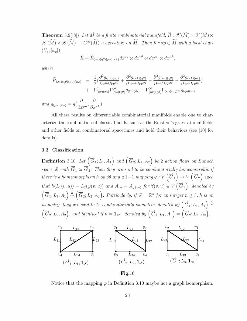
3.3 Classification

Definition 3.10 Let(−→G 1;L1, A1

)and

(−→G 2;L2, A2

)be 2 action flows on Banach

space B with−→G 1 ≃

−→G 2. Then they are said to be combinatorially homeomorphic if

there is a homeomorphism h on B and a 1−1 mapping ϕ : V(−→G 1

)→ V

(−→G 2

)such

that h(L1(v, u)) = L2(ϕ(v, u)) and Avu = Aϕ(vu) for ∀(v, u) ∈ V(−→G 1

), denoted by

(−→G 1;L1, A1

)h∼(−→G 2;L2, A2

). Particularly, if B = Rn for an integer n ≥ 3, h is an

isometry, they are said to be combinatorially isometric, denoted by(−→G 1;L1, A1

)h≃

(−→G 2;L2, A2

), and identical if h = 1Rn, denoted by

(−→G 1;L1, A1

)=(−→G 2;L2, A2

).- ?6 6-? - ?63 k sv1 v2

v3v4

L12

L23

L34

L41 L42

v2 v1v1 v2

v3 v4

L12

L43v3 v4

L21

L13

L34

L42L41 L42 L41L23

(−→G 1;L1, 1B) (

−→G 2;L2, 1B) (

−→G 3;L3, 1B)

Fig.16

Notice that the mapping ϕ in Definition 3.10 maybe not a graph isomorphism.

23

For example, the action flows(−→G 1;L1, 1Rn

)=(−→G 2;L2, 1Rn

)because there is a 1-1

mapping ϕ = (v1v2)(v3)(v4) : V(−→G 1

)→(−→G 2

)holding with L(u, v) = L(ϕ(u, v))

for ∀(u, v) ∈ E(−→G), which is not a graph isomorphism between

−→G 1 and

−→G 2 but

(−→G 1;L1, 1Rn

)6=

(−→G 3;L3, 1Rn

)for

−→G 1 6≃

−→G 3 in Fig.16. Thus if we denote by

Aut(−→G ;L,A

)all such 1-1 mappings ϕ : V

(−→G)→ V

(−→G)

holding with L(u, v) =

L(ϕ(u, v)) and Auv = Aϕ(uv) for ∀(u, v) ∈ E(−→G), then it is clearly a group itself

holding with the following result.

Theorem 3.11 If V(−→G)

= v1, v2, · · · , vp, then Aut(−→G ;L,A

)= Aut

−→G⊗

(Sp)−→G,

particularly, Aut(−→G ;L,A

)≻ Aut

−→G , where (Sp)−→G

is the stabilizer of symmetric

group Sp on ∆ = 1, 2, · · · , p.

For an isometry h on Rn, let(−→G ;L,A

)h

=(−→G ; hLh−1, A

)be an action flow,

i.e., replacing x1, x2, · · · , xn by h(x1), h(x2), · · · , h(xn). The result following is clearly

known by definition.

Theorem 3.12(−→G 1;L1, A1

)h≃(−→G 2;L2, A2

)if and only if

(−→G 1;L1, A1

)h

=(−→G 2;L2, A2

).

Certainly, we can also classify action flows geometrically. For example, two

finitely combinatorial manifolds M1, M2 are said to be homotopically equivalent

if there exist continuous mappings f : Ml → M2 and g : M2 → M1 such that

gf ≃identity: M2 → M2 and fg ≃identity: M1 → M1. Then we know

Theorem 3.13([7]) Let M1 and M2 be finitely combinatorial manifolds with an

equivalence : GL[M1 → GL[M2]. If for ∀M1,M2 ∈ V (GL[M1]), Mi is homo-

topic to (Mi) with homotopic mappings fMi: Mi → (Mi), gMi

: (Mi) → Mi

such that fMi|Mi

⋂Mj

= fMj|Mi

⋂Mj

, gMi|Mi

⋂Mj

= gMj|Mi

⋂Mj

providing (Mi,Mj) ∈

E(GL[M1]) for 1 ≤ i, j ≤ m, then M1 is homotopic to M2.

§4. Stable Action Flows

The importance of stability for a model on natural things P results in determining

the prediction and controlling of its behaviors. The same also happens to those of

24

action flows for the perturbation of things such as those shown in Fig.17 on operating

of the universe.

Fig.17

As we shown in Theorem 3.4, the Cauchy problem on partial differential equa-

tions of first order is uniquely G-solvable. Thus it is significant to consider the

stability of action flows. Let(−→G ;L(t), A

)be an action flow on Banach space B

with initial values(−→G ;L(t0), A

)and let ω :

(−→G ;L,A

)→ R be an index function.

It is said to be ω-stable if there exists a number δ(ε) for any number ε > 0 such that

∥∥∥ω(−→G ;L1(t) − L2(t), A

)∥∥∥ < ε,

or furthermore, asymptotically ω-stable if

limt→∞

∥∥∥ω(−→G ;L1(t) − L2(t), A

)∥∥∥ = 0

if initial values holding with

‖L1(t0)(v, u)− L2(t0)(v, u)‖ < δ(ε)

for ∀(v, u) ∈ E(−→G), for instance the norm-stable or sum-stable by letting

ω(−→G ;L,A

)=

∑

(v,u)∈E

(−→G)

∥∥∥LA+vu(v, u)

∥∥∥ .

Particularly, ;et

ω(−→G ;L, 1B

)=

∑

(v,u)∈E

(−→G)‖L(v, u)‖

or (−→G ;L,A

)= ‖

∑

(v,u)∈E

(−→G)L(v, u)‖, A 6= 1B.

25

The following result on the stability of−→G -flow solution was obtained in [17],

which is a commonly norm-stability on−→G -flows.

Theorem 4.1 Let V be the Hilbert space L2[∆]. Then, the−→G -flow solution X of

equation F (x, X,Xx1, · · · , Xxn, Xx1x2, · · ·) = 0

X|x0 =−→G

L

in−→G

V

is norm-stable if and only if the solution u(x) of equation

F (x, u, ux1, · · · , uxn, ux1x2, · · ·) = 0

u|x0 = ϕ(x)

on (v, u) is stable for ∀(v, u) ∈ E(−→G).

In fact, we only need to consider the stability of(−→G ;O, A

)after letting flows

0 = L(t)(v, u) − L(t)(v, u) on ∀(v, u) ∈ E(−→G)

without loss of generality.

Similarly, if there is a Liapunov ω-function L(ω(t)) : O → R, n ≥ 1 on−→G with

O ⊂ Rn open such that L(ω(t)) ≥ 0 with equality hold only if (x1, x2, · · · , xn) =

(0, 0, · · · , 0) and if t ≥ t0, L(ω(t)) ≤ 0, then it can be likewise Theorem 3.8 of [12]

to know the next result, where L(ω) =dL(ω)

dt.

Theorem 4.2 If there is a Liapunov sum-function L(ω(t)) : O → R on−→G , then(

−→G ;O, A

)is ω-stable, and furthermore, if L(ω(t)) < 0 for

(−→G ;L(t), A

)6= O, then

(−→G ;O, A

)is asymptotically ω-stable.

For example, let(−→G ;L,A

)be the action flow with operators Azi+1zi = −

d

dtfor z = v, u, · · · , w and A+

vivi+1= λ1i, A

+uiui+1

= λ2i, · · ·, A+wiwi+1

= λni for integer

i ≡ (modn), such as those shown in Fig.18.- ?6 - ?6 - ?66v1 v2

v3vn

u1 u2

u3un

w1 w2

w3wn

x1

x1x1

x1x1

x2

x2

x2

x2

x2

xn

xn

xnxn

xn

Fig.18

26

Then its conservation equations are respectively

x1 = λ11x1

x1 = λ12x1

· · · · · · · · ·

x1 = λ1nx1

,

x2 = λ21x2

x2 = λ22x2

· · · · · · · · ·

x2 = λ2nx2

, · · · ,

xn = λn1xn

xn = λn2xn

· · · · · · · · ·

xn = λnnxn

,

where all λij, 1 ≤ i, j ≤ n are real and λij1 6= λij2 if j1 6= j2 for integers 1 ≤ i ≤ n.

Let L = x21 + x2

2 + · · · + x2n. Then L = λi11x

21 + λi22x

22 + · · · + λinnx

2n for integers

1 ≤ i ≤ n, where 1 ≤ ij ≤ n for integers 1 ≤ j ≤ n. Whence, it is a Liapunov

ω-function for action flow(−→G ;L,A

)if λij < 0 for integers 1 ≤ i, j ≤ n.

§5. Applications

As a powerful theory, action flow extends classical mathematics on embedded graph,

which can be used as a model nearly for moving things in the nature, particularly,

applying to physics and mathematical ecology.

5.1 Physics

For diversity of things, two typical examples are respectively the superposition be-

havior of microcosmic particle and the quarks model of Sakata, or Gell-Mann and

Ne’eman by assuming internal structures of hadrons and gluons, which can not be

commonly understanding.

63Yo o 7ψ1 ∈ V1

ψ11 ∈ V11 ψ12 ∈ V12

ψ31 ∈ V31

ψ32 ∈ V32ψ33 ∈ V33 ψ34 ∈ V34

Fig.19

Certainly, H.Everett’s multiverse interpretation in Fig.6 presented the superposition

of particles but with a little machinery, i.e., viewed different worlds in different

quantum mechanics and explained the superposition of a particle to be 2 branch

27

tree such as those shown in Fig.19, where the multiverse is⋃i≥1

Vi with Vkl = V for

integers k ≥ 1, 1 ≤ l ≤ 2k but in different positions.

Similarly, the quark model assumes internal structures K2, K3 respectively on

hadrons and gluons mechanically for hold the behaviors of particles. However, such

an assumption is a little ambiguous in logic, i.e., we can not even conclude which

is the point, the hadron and gluon or its subparticle, the quark. However, the

action flows imply the rightness of H.Everett’s multiverse interpretation, also the

assumption of physicists on the internal structures for hold the behaviors of particles

because there are infinite many such graphs−→G satisfying conditions of Theorem 2.9.

P Pψ1ψ2ψN ψ−11 ψ−1

2 ψ−1N

-Particle Antiparticle

Fig.20

For example, let−→G =

−→B n or

−→D⊥

0,2N,0, i.e., a bouquet or a dipole. Then we can

respectively establish a−→G -flow model for fermions, leptons, quark P with an an-

tiparticle P , and the mediate interaction particles quanta presented in Banach space−→B

V

N or−→D⊥

V

0,2N,0, such as those shown in Figs.20 and 21,

P P

ψN

2

2

1

1

ψN

ψ

ψ

ψ

ψ

−→D⊥

Lψ

0,2N,0

Fig.21

where, the vertex P, P ′ denotes particles, and arcs or loops with state functions

ψ1, ψ2, · · · , ψN are its states with inverse functions ψ−11 , ψ−1

2 , · · · , ψ−1N . Notice that

−→B

Lψ

N and−→D⊥

Lψ

0,2N,0 both are a union of N circuits. We know the following result.

28

Theorem 5.1([18]) For any integer N ≥ 1, there are indeed−→D⊥

Lψ

0,2N,0-flow solution

on Klein-Gordon equation (3.5), and−→B

Lψ

N -flow solution on Dirac equation (3.6).

For a particle P consisted of l elementary particles P1, P1, · · · , Pl underlying a

graph−→G[P], its

−→G -flow is obtained by replace vertices v by

−→B

LψvNv

and arcs e by

−→D⊥

Lψe

0,2Ne,0 in−→G[P], denoted by

−→G

Lψ[−→B v,

−→D e

]. Then we know that

Theorem 5.2([18]) If P is a particle consisted of elementary particles P1, P1, · · · , Pl,

then−→G

Lψ[−→B v,

−→D e

]is a

−→G -flow solution on the Schrodinger equation (1.1) whenever

its size index λG is finite or infinite, where

λG =∑

v∈V

(−→G)Nv +

∑

e∈V

(−→G)Ne.

5.2 Mathematical Ecology

Action flows can applied to be a model of ecological systems. For example, let u and

v denote respectively the density of two species that compete for a common food

supply. Then the equations of growth of the two populations may be characterized

by ([6]) u = M(u, v)u

v = N(u, v)v(5.1)

particularly, the Lotaka-Volterra competition model is given by

u = a1u (1 − u/K1 − α12v/K1)

v = a2v (1 − v/K2 − α21u/K2)(5.2)

in ordinary differentials ([21]), or

ut = d1∆u+ a1u(1 −K1u− α12v/K1)

vt = d2∆v + a2v(1 −K2u− α21v/K2)(5.3)

in partial differentials on a boundary domain Ω ⊂ Rn for an integer n ≥ 1 with initial

conditions∂u

∂ν=

∂v

∂ν= 0 on unit normal out vector ν, u(x, 0) = u0(x), v(x, 0) =

v0(x) ([28]), where u(x, t), v(x, t) are respectively the density of 2 competitive species

at (x, t) ∈ Ω × (0,∞), M,N and positive parameters a1, a2 are the growth rates,

K1, K2 are the carrying capacities, αij denotes the interaction between the two

29

species, i.e., the effect of species i on species j for i, j = 1 or 2, and d1, d2 are the

diffusion rate of species 1 and 2, respectively. This system is nothing else but an

action flow on loop B1 on a boundary domain Ω ⊂ Rn for an integer n ≥ 1

6(u, v) ∂/∂t

AO

Fig.22

with initial conditions∂u

∂ν=

∂v

∂ν= 0 on unit normal out vector ν and u(x, 0) =

u0(x), v(x, 0) = v0(x) for (x, t) ∈ Ω × (0,∞) such as those shown in Fig.22, where

A(u, v) = (uM(u, v), vN(u, v)). For example, M(u, v) = a1 (1 − u/K1 − α12v/K1),

N(u, v) = a2 (1 − v/K2 − α21u/K2) in equations (5.2) orM(u, v) = d1∆u/u+a1(1−

K1u− α12v/K1), N(u, v) = d2∆v/v+ a2(1−K2u− α21v/K2) in equations (5.3) for

∀(x, t) ∈ Ω × (0,∞).

Similarly, assume there are four kind groups in persons at time t, i.e., susceptible

S(t), infected but in the incubation period E(t), infected with infectious I(t) and

recovered R(t) and new recognition Λ with removal rates κ, α, contact rate β and

natural mortality rate µ, such as the action flow shown in Fig.23.-?6 R I I)

v1

v2 v3

v4

O

S

Λ

−µS

d/dt

βSI

E

−µE

d/dt

κE

αI

I

−µI

d/dt

R

−µR +N

d/dt

Fig.23

Then, we are easily to get the SEIR model on infectious by conservative laws re-

30

spectively at vertices v1, v2, v3 and v4 following:

S = Λ − µS − βSI

E = βSI − (µ+ κ)E

I = κE − (µ+ α)I

R = αI − µR

(5.4)

where, N = S+R+E+ I−µ(S+R+E+ I) and all end-operators are 1 if it is not

labeled in Fig.23. Notice that the systems (5.1)-(5.4) of differential equations are

solvable. Whence, the behavior of action flows in Figs.22 and 23 can be characterized

respectively by solution of system (5.1)-(5.4).

Generally, an ecological system is such an action flow(−→G ;L,A

)on an oriented

graph with a loop on its each vertex, where flows on loops and other edges denote

respectively the density of species or interactions of one species action on another. If

the conservation laws of an action flow are not solvable, then holding on the reality

of competitive species by solution of equations will be not suitable again.-6 6(u, v) (u, v)A1 A2

∂/∂t ∂/∂tO1 O2

(U, V )

Fig.24

For example, the action flow shown in Fig.24 is such an ecological system with

conservation lawsut = A1(u, t) + U(u, t)

vt = A1(u, t) + V (u, t),

ut = A2(u, t) − U(u, t)

vt = A2(u, t) − V (u, t)

under initial conditions∂u

∂ν=∂v

∂ν= 0, u(x, 0) = u0(x), v(x, 0) = v0(x) for (x, t) ∈

Ω × (0,∞), where

A1(u, v) = (d1∆u+ a1u(1 −K1u− α12v/K1), d2∆v + a2v(1 −K2u− α21v/K2))

A2(u, v) = (d3∆u+ a3u(1 −K3u− α34v/K3), d4∆v + a4v(1 −K4u− α43v/K4))

for ∀(x, t) ∈ Ω × (0,∞) and U, V are known functions. They are non-solvable in

general but we can characterize its behaviors, for instance, the global stability by

application of Theorem 4.2.

31

In fact, all ecological systems are interaction fields in physics. Let C1,C2, · · · ,Cm

be m interaction fields with respective Hamiltonians H [1], H [2], · · · , H [m], where

H [k] : (q1, · · · , qn, p2, · · · , pn, t) → H [k](q1, · · · , qn, p1, · · · , pn, t)

for integers 1 ≤ k ≤ m, i.e.,

∂H [k]

∂pi

=dqidt

∂H [k]

∂qi= −

dpi

dt, 1 ≤ i ≤ n

1 ≤ k ≤ m.

Such a system is equivalent to the Cauchy problem on the system of partial differ-

ential equations

∂u

∂t= Hk(t, x1, · · · , xn−1, p1, · · · , pn−1)

u|t=t0 = u[k]0 (x1, x2, · · · , xn−1)

1 ≤ k ≤ m. (PDESm)

and is in fact an action flows on m dipoles−→D 0,2,0. For example, a system of inter-

action field is shown in Fig.25 in m = 4 with A = A′ =∂

∂tand A1 = A1 = 1.- - - -u

H1

u

H2

u

H3 H4

uA A′

A1A′1

A

A′1

A′

A1

A

A′1

A′

A1

A

A′1

A′

A1

Fig.25

By choosing Liapunov sum-function L(ω(t))(X) =m∑

i=1

Hi(X) on−→G in Theorem

3.15, the following result was obtained in [15] on the stability of system (PDESm).

Theorem 5.3 Let X[i]0 be an equilibrium point of the ith equation in (PDESm) for

each integer 1 ≤ i ≤ m. Ifm∑

i=1

Hi(X) > 0 andm∑

i=1

∂Hi

∂t≤ 0 for X 6=

m∑i=1

X[i]0 , then the

system (PDESm) is sum-stability, i.e., G[t]Σ∼ G[0]. Furthermore, if

m∑i=1

∂Hi

∂t< 0

for X 6=m∑

i=1

X[i]0 , then G[t]

Σ→ G[0].

§6. Conclusion

The main function of mathematics is provide quantitative analysis tools or ways

for holding on the reality of things by observing from a macro or micro view. In

32

fact, the out or macro observation is basic but the in-observation is cardinal, and an

in-observation characterizes the individual behavior of things but with non-solvable

equations in mathematics. However, the trend of mathematical developing in 20th

century shows that a mathematical system is more concise, its conclusion is more

extended, but farther to the true face of the natural things. Is a mathematical

true inevitable lead to the natural reality of a thing? Certainly not because more

characters of thing P have been abandoned in its mathematical model. Then, is

there a mathematical envelope theory on classical mathematics reflecting the nature

of things? Answer this question motivates the mathematical combinatorics, i.e.,

extending mathematical systems on topological graphs−→G because the reality of

things is nothing else but a multiverse on a topological structure under action, i.e.,

action flows, which is an appropriated way for understanding the nature because

things are in connection, also with contradiction.

References

[1] R.Abraham and J.E.Marsden, Foundation of Mechanics (2nd edition), Addison-

Wesley, Reading, Mass, 1978.

[2] John B.Conway, A Course in Functional Analysis, Springer-Verlag New York,Inc.,

1990.

[3] M.Carmeli, Classical Fields–General Relativity and Gauge Theory, World Sci-

entific, 2001.

[4] Fritz John, Partial Differential Equations, New York, USA: Springer-Verlag,

1982.

[5] H.Everett, Relative state formulation of quantum mechanics, Rev.Mod.Phys.,

29(1957), 454-462.

[6] Morris W.Hirsch, Stephen Smale and Robert L.Devaney, Differential Equations,

Dynamical Systems & An introduction to Chaos (Second Edition), Elsevier (Sin-

gapore) Pte Ltd, 2006.

[7] Linfan Mao, Combinatorial speculation and combinatorial conjecture for math-

ematics, International J.Math. Combin. Vol.1(2007), No.1, 1-19.

[8] Linfan Mao, Geometrical theory on combinatorial manifolds, JP J.Geometry

and Topology, Vol.7, No.1(2007),65-114.

33

[9] Linfan Mao, Combinatorial fields-an introduction, International J. Math.Combin.,

Vol.1(2009), Vol.3, 1-22.

[10] Linfan Mao, Relativity in combinatorial gravitational fields, Progress in Physics,

Vol.3(2010), 39-50.

[11] Linfan Mao, Combinatorial Geometry with Applications to Field Theory, The

Education Publisher Inc., USA, 2011.

[12] Linfan Mao, Global stability of non-solvable ordinary differential equations with

applications, International J.Math. Combin., Vol.1 (2013), 1-37.

[13] Linfan Mao, Non-solvable equation systems with graphs embedded in Rn, Pro-

ceedings of the First International Conference on Smarandache Multispace and

Multistructure, The Education Publisher Inc. July, 2013

[14] Linfan Mao, Geometry on GL-systems of homogenous polynomials, Interna-

tional J.Contemp. Math. Sciences, Vol.9 (2014), No.6, 287-308.

[15] Linfan Mao, Mathematics on non-mathematics - A combinatorial contribution,

International J.Math. Combin., Vol.3(2014), 1-34.

[16] Linfan Mao, Cauchy problem on non-solvable system of first order partial dif-

ferential equations with applications, Methods and Applications of Analysis,

Vol.22, 2(2015), 171-200.

[17] Linfan Mao, Extended Banach−→G -flow spaces on differential equations with

applications, Electronic J.Mathematical Analysis and Applications, Vol.3, No.2

(2015), 59-91.

[18] Linfan Mao, A new understanding of particles by−→G -flow interpretation of dif-

ferential equation, Progress in Physics, Vol.11(2015), 193-201.

[19] Linfan Mao, A review on natural reality with physical equation, Progress in

Physics, Vol.11(2015), 276-282.

[20] Linfan Mao, Mathematics after CC conjecture – combinatorial notions and

achievements, International J.Math. Combin., Vol.2(2015), 1-31.

[21] C.Neuhauser, Mathematical challenges in spatial ecology, Notices in AMS,

Vol.48, 11(2001), 1304-1414.

[22] Quang Ho-Kim and Pham Xuan Yem, Elementary Particles and Their Inter-

actions, Springer-Verlag Berlin Heidelberg, 1998.

[23] F.Smarandache, Paradoxist Geometry, State Archives from Valcea, Rm. Valcea,

Romania, 1969, and in Paradoxist Mathematics, Collected Papers (Vol. II),

34

Kishinev University Press, Kishinev, 5-28, 1997.

[24] F.Smarandache, A new form of matter – unmatter, composed of particles and

anti-particles, Progess in Physics, Vol.1(2005), 9-11.

[25] F.Smarandache and D.Rabounski, Unmatter entities inside nuclei, predicted by

the Brightsen nucleon cluster model, Progress in Physics, Vol.1(2006), 14-18.

[26] J.Stillwell, Classical Topology and Combinatorial Group Theory, Springer-Verlag,

New York Inc., 1980.

[27] Wolfgang Walter, Ordinary Differential Equations, Springer-Verlag New York,Inc.,

1998.

[28] Y.Lou, Some reaction diffusion models in spatial ecology (in Chinese), Sci.Sin.Math.,

Vol.45(2015), 1619-1634.

35

Linfan Mao is a researcher of Chinese Academy of Mathemat-

ics and System Science, the president of Academy of Mathemat-

ical Combinatorics & Applications (AMCA), an honorary mem-

ber of Neutrosophic Science International Association (USA),

an adjunct professor of Beijing University of Civil Engineering

and Architecture, the editor-in-chief of International Journal of

Mathematica Combinatorics, also a deputy general secretary of

the China Tendering & Bidding Association in Beijing. He got his Ph.D in North-

ern Jiaotong University in 2002 and finished his postdoctoral report for Chinese

Academy of Sciences in 2005. His research interest is mainly on mathematical com-

binatorics and Smarandache multi-spaces with applications to sciences, includes

combinatorics, algebra, topology, differential geometry, theoretical physics, parallel

universe, ecology and bidding theory. Now he has published more than 70 papers

and 9 books on mathematics with applications on these fields, such as those of Auto-

morphism Groups of Maps, Surfaces and Smarandache Geometries, Combinatorial

Geometry with Applications to Field Theory and Smarandache Multi-Space Theory,

3 books on mathematics by The Education Publisher Inc. of USA in 2011.