Embed Size (px)
Citation preview

Mathematics for Economics
MA/MSSc in Economics-2019/2020
Prof. W. M. Semasinghe
Department of Economics

MATHEMATICS AND STATISTICS
LERNING OUTCOMES:
By the end of this course unit students will be able to demonstrate skills in mathematical
and statistical methods that are highly useful in analyzing problems related to economic
theory and practice and understand the uses of basic descriptive and inferential statistics in
economic analysis.
COURSE CONTENTS: This course unit consists of two parts:
Part I: Mathematics - Functions and their applications in economics, Calculus and its
applications in economics: Differentiation, Partial differentiation, Integration; Matrices;
Maxima and Minima; Constrained Optimization with economic applications, Linear
programming.
Part II: Statistics - Probability and probability Theory; continuous and discrete variables,
continuous and discrete variables distributions, Joint distributions; Moment generating
functions; Hypothesis testing and confidence intervals.

Y%z; (Functions)
Y%s;hla hkq úp,H w;r iïnkaO;dj úia;r lsrSug fhdod .kakd Wml%uhls'
y hk úp,Hfha w.h x hk ;j;a úp,Hhl w.h u; r|d mj;S kï yúp,Hh x úp,Hfha Y%s;hls'
y = f (x)
x úp,H .kakd w.h wdodk ixLHd (input numbers)
y úp,H .kakd w.h m%;sodk ixLHd (output numbers)
Y%s;hl tla tla wdodk ixLHdj i|yd tla m%;sodk ixLHdjla muKla .kS'
Y%s;hla hkq ztla wdodk ixLHdjlg yrshgu tla m%;sodk ixLHdjla mejfrk f,i w¾: olajk ,o kS;shlsZ'

Y%s;fha jiu( w¾: olajk ,o kS;sh ;Dma; flfrk ish¨u wdodk ixLHd ldKavh Y%s;fha jiu (domain of the function) f,i ye¢kafõ'
mrdih ish¨u m%;sodk ixLHd ldKavh Y%s;fha mrdih (range of the function)
f,i ye¢kafõ'
úfYaIfhka i|yka l<fyd;a yer yeu úgu Y%s;fha jiu ;d;aúl ixLHdj,skaiukaú; fõ'
Y%s;hl wdodk ixLHd ksrEmkh lrk úp,Hh iajdh;a; úp,H f,i (independent variables) ye¢kafõ'
m%;sodk ixLHd ksrEmkh lrk úp,Hh mrdh;a; úp,H f,i (dependent
variables) ye¢kafõ' y = f(x)
mrdh;a; úp,H iajdh;a; úp,H

q = f(p) s = f(yd)
p = f(q) c = f (yd)
TC = f(q) TR = f(q)
y yd z, x úp,Hfha Y%s; kï
F, G, g, h, θ, φ, ψ, Φ, Ψ hkdoz ixfla; o fhdod .kS
Y%s;Sh iïnkaO;d i|yd ksoiqka
y = y(x) yd z = z(x)
y = f(x) iy z = f(x)

fuyz x úp,Hh 1 yer ´kEu ;d;aúl ixLHdjla jk úg y ;d;aúl ixLHdjla fõ'
Y%z;fha jiu 1 yer TAkEu ;d;aúl ixLHdjlz R – {1} or x≠1
x wdodk ixLHdj ´kEu ;d;aúl ixLHdjla jk úg y m%;zodk ixLHdj o ;d;aúl ixLHdjla fõ' túg Y%z;fha jiu ;d;aúl ixLHd ldKavhlz R
1
32
x
xyeg. 2
eg. 1 y = f(x) = 18x – 3x2
eg. 3. )9(
6
xxy
Y%s;fha yrh x ≠ 0 iy x ≠ -9 úh hq;= h'
Y%z;fha jiu 0 yd 1 yer ´kEu ;d;aúl ixLHd ldKavhlz

x wdodk ixLHdj ´kEu ;d;aúl ixLHdjla jk úg y m%;zodk ixLHdj o ;d;aúl ixLHdjla fõ' Y%z;fha mrdih ;d;aúl ixLHd ldKavhlz R
mrdih fidhkak
1). y = 2x
2). y = x2,
Y%s;fha jiu ´kEu ;d;aúl ixLHdjla jk úg mrdih y ≥ 0
3). y = -5x, (-1 ≤ x ≤ 2)
mrdih -10 ≤ y ≤ 5

fndfyda wd¾Ól úoHd;aul úp,H iajNdjfhkau hï iSudjla ;=< msysá Y+kH fkdjk w.h .kS'
wd¾Ól úoHd;aul wdlD;sj, jiu tlS iSudj ;=< msysghs'
kso(
wdh;khl uq`M msßjeh ffoksl ksIamdos;fha (q), C =150 + 7q wdldrfha Y%s;hls'
wdh;kfha ksIamdok ksIamdok Odß;dj osklg tall100ls'
msßjeh Y%s;fha jiu yd mrdih l=ula fõ o@
1000| qqDomain
850150| CCRange

a hkq f(x) Y%s;fha x yz hï kzYaÑ; w.hla kï x = a jk úg Y%z;fha w.h f(a)
f,i olajhz
xy = f(x) =
7x + 1
f(a) = a/(7a + 1)
f(4) = 4/ 29
eg. 1
Given,
f(x) = x2 + 5x – 6 Find, f(3) and f(-4)
7
17924)(
x
xxxf Find, f(5) and f(-2)
4
112)(
x
xxf Find, f(3a) and f(a - 4)

Types of Functions
Constant function: mrdih ksh;hlska$tla w.hlska muKla iukaú; Y%s;
y = 7
f(x) = 10
x ys w.h ljrla jqj o Y%s;fha w.h fkdfjkiaj mj;S
fujeks Y%s;hla oaùudk ;,hl ;sria wCIhg iudka;r ir, f¾Ldjls
cd;sl wdodhï wdlD;shl wdfhdack nys¾ckH úp,Hhls' y
0 I
I = f(y)

nyq mo Y%z; (Polynomial Functions)
General form of a Polynomial Functions of Degree n
f(x) = a0 + a1x + a2x2 + ……..+ an-1x
n-1 + anxn
n Ok ksÅ,hlz. a0 …..an kzh; mo jk w;r an ≠ 0
e.g. f(x) = 8x6 + 3x4 – x3 + 5x2 + 2x + 3 (polynomial of degree 6)
f(x) = x8 + 2x5 + 3x4 + 7x2 + 6x – 5 (polynomial of degree 8)
nyqmo Y%z;fha n kzÅ,fha w.h u; ;ZrKh jk úúO iajrEmfha nyqmo Y%z;
when
n = 0 y = a0 Constant function
n = 1 y = a0 + a1x Linear function (polynomial of degree 1)
n = 2 y = a0 + a1x + a2x2 Quadratic function
n = 3 y = a0 + a1x + a2x2 + a3x
3 Cubic function

mrzfïh Y%z; Rational Functions
)(
)()(
xh
xgxf wdldrfha Y%s; mrsfïh Y%s; fõ' fuys g(x) yd h(x) nyqmo Y%z; jk w;r
h(x) ≠ 0 fõ'
f(x), x ys nyqmo Y%z; foll wkqmd;hla jYfhka oelafõ'
)12(
)53)(
2
x
xxf
ixhqla; Y%z; Composite Function or Function of a Function
y = g(u) yd u = f(x) kuA y = g[f(x)]
eg. (1). If y = u2 + 3 and u = 2x + 1 then,
y = (2x+1)2 + 3
eg. (2). If y = x3 - 3x + 5 and x = ½√t + 3 then,
y = (½√t+3)3 – 3(½√t+3) +5

Functions of Two or More independent variable
z = f(x, y)
z = ax + by
v = f(L, K)
z = a0 + a1x + a2x2 + b1y + b2y
2
y = a1x1 + a2x2 + a3x3 + ….anxn
Non-algebraic Functions
y = bx ,
y = et
y = logbx
y = lnx
wdldrfha >d;Zh Y%z; iy
wdldrfha ,>q.Kl Y%z;

wjl,kh (Differentiation)
Y%s;hl iajdh;a; úp,Hfha b;d l=vd fjkilg m%;spdr jYfhka mrdh;a; úp,Hfha we;sjk fjki fiùu wjYH fõ' ta i|yd wjl,kh Ndú; l< yels h'
fokq ,enQ Y%s;hl wjl,k ix.=Klh (differential coefficient) fyj;a jHq;amkakh (derivative) fiùfï l%shdj,sh wjl,kh (differentiation) kï fõ'
y = f(x) Y%s;fha x úp,Hh b;d l=vd m%udKhska fjkia jk úg y úp,Hfha we;sjk fjki y = f(x) Y%s;fha x úIfhys y wjl,kh lsÍfuka ,efí'
y = f(x) Y%s;fha x úIfhys yys wjl,k ix.=Kh my; mßos w¾: oelaúh yels h'
x
ylimx
x
f(x) - x)f(x limx
dx
dy
00
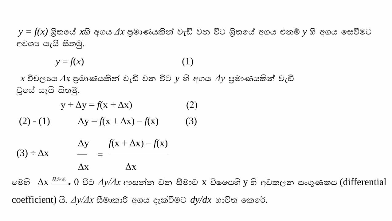
y = f(x) Y%s;fha xys w.h Δx m%udKhlska jeä jk úg Y%s;fha w.h tkï y ys w.h fiùug wjYH hehs is;uq'
y = f(x) (1)
x úp,Hh Δx m%udKhlska jeä jk úg y yz w.h Δy m%udKhlzka jeäjQfha hehz iz;uq'
Δy f(x + Δx) – f(x)
=
Δx Δx
y + Δy = f(x + Δx) (2)
(2) - (1) Δy = f(x + Δx) – f(x) (3)
(3) ÷ Δx
fuyz Δx iSudj 0 úg Δy/Δx wdikak jk iSudj x úIfhyz y yz wjl,k ix.=Klh (differential
coefficient) hz' Δy/Δx iSudldÍ w.h oelaùug dy/dx Ndú; flf¾'

eg. y = 3x2 + 2 ……………….. (1)
Suppose that x increased by Δx, as a result y is increased by Δy, then
y + Δy = 3(x + Δx)2 + 2
= 3(x2+2xΔx+Δx2) + 2
y + Δy = 3x2 + 6xΔx + 3Δx2 + 2 ……. (2)
(2) – (1) Δy = 6xΔx + 3Δx2 …………(3)
(3) ÷ Δx Δy/Δx = 6x + 3Δx
lim Δy/Δx = 6xΔx→ 0

Rules of Differentiation
(1) Constant function rule
y = 9x + 6
(2) Linear function rule
0)()(
xfdx
kd
dx
dy0)(
)10( xf
dx
d
dx
dy
y = f(x) =10
kdx
kxd
dx
dy
)2( 9)69(
dx
xd
dx
dy
y = f(x) = k
y = f(x) = kx + 2
u, v yd y hkq x yz Y%z;hka o k hkq kzh;hla o jk úg

y = f(x) = xn
(3) Power function rule
1)( nn
nxdx
xd
dx
dy

(4). Generalized power function rule
y = kxn
1)( nn
nkxdx
kxd
dx
dyn
n
axndx
axd
dx
dy)1(
)( 1
eg. y = axn+1
eg. y = 1/x
21)(
xdx
xd
dx
dy

(5). Sum-difference rule
)]()([ xgxfy
dx
xgd
dx
xfd
dx
dy )]([)]([

(6). Function of a function rule
y = f(u) iy u = g(x), jk úg y = f[g(x)] Y%s;hl Y%s;hla fõ'
y, u úIfhys wjl,kh l< yels Y%s;hla o u, x úIfhys wjl,kh l< yels Y%s;hla o jk úg y = f[g(x)], x úIfhys wjl,kh l< yels Y%s;hla fõ'
fujeks Y%s;hl dy/dx ,nd .ekSu fowdldrhlg mq`Mjk
1). y, x j,ska m%ldY lr wjl,kh lsÍu
e.g. y = u2+3 iy u = 2x+1, jk úg y = (2x+1)2 + 3 = 4x2+4x+4
48dx
dy x

2). tla tla Y%s;h fjk fjku iajdh;a; úp,Hh úIfhys wjl,kh lr odu kS;sh (chain
rule) fhdod .ekSu
dx
du
du
dy
dx
dy
2 and 2du
dy
dx
duu
48)12(44dx
dy xxu
dx
du
du
dy
by; Y%s;fha wjl,k ix.=Klh

When y = [f(x)]n
We can express this procedure as rule as follows:
ex. y = (ax+b)n
If we defined (ax + b) = u then y = un
1
du
dy nnu a
dx
baxd
)(
dx
dy and
11 )()(dx
dy nn baxanabaxn
dx
du
du
dy
)()]([dx
dy 1 xfxfn n

(7). Product rule
y = [f(x).g(x)]
f(x) = u and g(x) = v
y = uv
dx
xfdxg
dx
xdgdxf
dx
dy )]([)(
)]([)(
dx
duv
dx
dvu
dx
dy

(8). Quotient rule
Defining f f(x) = u g(x) = v
)(
)(
xg
xfy
2)]([
)]([)(
)]([)(
xg
dx
xgdxf
dx
xfdxg
dx
dy
v
uy
2)(
)()(
v
dx
vdu
dx
udv
dx
dy

When y = 1/f(x)
2)(
)(
xf
xf
dx
dy
eg. y = 1/ (x2+1)
22 1
2
x
x
dx
dy

10. Exponential function rule
iajdh;a; jzp,Hh >d;hla jYfhka mzyzgk Y%z;hla ‘>d;’h Y%z;hla’ (Exponential function) f,i y#-qkajhz"
nyqmo Y%z;hl iajdh;a; jzp,Hfha n,h ‘>d;h’ (exponent) f,i y#-qkajk w;r th kzh;hlz'
eg. y = f(x) = bx (b>1)
fuyz y yd x mz<zfj,zka mrdh;a; yd iajdh;a; jzp,H jk w;r b u.ska oelafjkafka >d;fha mdoh (base) hz'
l,kfha oZ .Kz;uh l%zhdldrluAj, myiqj i#oyd e kuA jk wmrzfuAh ixLHdj (e =2.71828…)
>d;fha mdoh f,i fhdod .kZ'
eg. y = ex y = e3x y = Aerx
Wod: y = 2x3 + 4x2 + 5

Ex. (1) y = ex
dy = ex
dx
dy du= eu
dx dx
Ex.( 2) y = eu yd u = f(x) kuA
eg. (3) y = e(3x + 2)
dy= 3e(3x + 2)
dx

11. Log-function rule
úp,Hhla ;j;a úp,Hhl ,>q.Klfha Y%z;hla jYfhka m%ldY flfrk Y%z;hla ,>q Y%z;hla
(Log function or Logarithmic function) f,i ye#ozkafõ'
y = logbx
fmr oZ oela jQ mrzoz l,kfha oZ ,>q.Klfha mdoh jYfhka .kafka e h'
• e mdohg ,>q m%lD;s ,>q (natural logarithm) f,i y#-qkajk w;r th loge fyda ln u.zka ixfla;j;a lrhz'
y = loge 2x fyda y = ln 2x

1. y = ln x
3. If y = ln u and u = f(x)
2. y = k(ln x)
xdx
xd
dx
dy 1)(ln
x
k
xk
dx
xdk
dx
dy
1)(ln
dx
du
udx
dy
1
Ex. y = ln (3x2 + 5))53(
66
)53(
1
22
x
xx
xdx
dy
y = ln xn dy 1 n= nxn-1 =
dx xn x

Y%z;hl jHq;amkakh Y%z;hla jk jzg jHq;amkakhg o jHq;amkakhla we;'
Higher Order Derivatives
y = f(x) yz jHq;amkakh tyz m%:u jHq;amkakh (first derivative) hz' th dy/dx fyda f '(x)
f,i olajhz'
f '(x)yz jHq;amkakh d2y/dx2 fyda f ''(x) f,i olajhz' th f(x) yz fojk jHq;amkakhhz'
y = f(x) kuA
1st derivative:
2nd derivative:
dx
dy
dx
ydxf
)()(
2
2)/()(
dx
yd
dx
dxdydxf
3rd derivative:
nth derivative:
3
322 )/()(
dx
yd
dx
dxyddxf
n
nnnn
dx
yd
dx
dxyddxf
)/()(
11

eg. y = x4 + 3x2 – 2x + 7
1st derivative:
3rd derivative:
2nd derivative:
Find
nd2 21 . xxyi
rd3 2
13 .
x
xyii
264)( 3 xxdx
dyxf
612)( 2
2
2
xdx
ydxf
xdx
ydxf 24)(
3
3

wdxYzl wjl,kh Partial differentiation
fï olajd i,ld n,k ,oafoa fmd-qfõ f(x) jYfhka oela jQ ;kz iajdh;a;
úp,Hhla iyz; Y%z; mz<zn#oj h' tfy;a fndfyda úg iajdh;a; úp,H tllg
jeä ixLHdjla mj;akd wjia:d mz<zn#o i,ld ne,Zug iz-q fõ'
x yd y hk iajdh;a; úp,H fol iyz; Y%z;hla
z = f(x, y) f,i oelaúh yelzh' z mrdh;a; úp,Hhhz'
y hkq x1, x2, …xn kï jQ iajdh;a; úp,H n ixLHdjl Y%z;hla kï
y = f(x1, x2, …., xn) f,i oelaúh yelzh'

fujekz nyq úp,H Y%z;hl" wfkl=;a úp,H fkdfjkiaj ;zìh oZ tla iajdh;a;úp,Hhla b;d l=vd m%udKhlzka fjkia jk úg Y%z;fha w.h fiùug wjYHfõ' fï i#oyd wdxYzl wjl,kh kï Yz,amZh l%uh Ndú; lrhz‘
ta wkqj y = f(x1, x2, …., xn) kï nyq úp,H Y%z;hl wfkl=;a úp,H ia:djrj;zìh oZ tla iajdh;a; úp,Hhl fjkia ùug wkqrEmj y fjkia jk wkqmd;hwdxYzl wjl,fhka (partial derivative) uek olajhz'
z = f(x, y) hk Y%z;fha x úIfhyz z yz wdxYzl wjl,h .ekSfïoS y ksh;hla f,i
i<lk w;r th ∂z/∂x fyda fx u.zka kzrEmkh lrhz'
y úIfhyz z yz wdxYzl wjl,h .ekSfïoS x ksh;hla f,i i<lk w;r th ∂z/∂y fyda fy u.zka kzrEmkh lrhz'

ex. (1) y = f(x1,x2) = 3x12 + x1x2 + 4x2
2
)2)(7(),( 2 xyxyxfzex. (2).

ex. (3). If f(x,y) = (2x – 3y)/(x + y) Find fx and fy

^2& mdrzfNdaclhl=f.a WfmaCId jl%fha wdldrh U = U(x1, x2) = (x1 + 2)2 (x2 + 3)2
fuyz U uq#M Wmfhda.Z;dj o x1 yd x2 NdKav foflyz m%udK o olajhz'i. NdKav foflyz wdka;zl Wmfhda.Z;d Y%z; jHq;amkak lrkak'ii. NdKav foflka tall 3 ne.zka mrzfNdackh lrkafka kuA m<uq NdKavfha
wdka;zl Wmfhda.Z;dj .Kkh lrkak'
wNHdi ^1& my; oelafjk Y%z;j, wdxYzl wjl, (fx yd fy) w.hkak'
i. z = ln (x2 + y2)
ii. z = (x + y) e(x + y)
iii.z = 3x2y + 4xy2 + 6xy
(3) V = ALαKβ hk kzIamdok Y%z;fha L yd K hkq Y%uh yd m%d.aOkh o v hkq kzuejqu o fjA' Y%ufha yd m%d.aOkfha wdka;zl M,odj .Kkh lrkak'

(4) The cost function of a firm is given by C =2x2 +x– 5. Find (i) the average
cost (ii) the marginal cost, when x = 4
(5) The total revenue received from the sale of x units of a product is given by
R(x) =12x+2x2+6.
Find (i) the average revenue
(ii) the marginal revenue
(iii) marginal revenue at x = 50
(iv) the actual revenue from selling 51st item
(6) The demand function of a product for a manufacturer is p (x) = ax + b
He knows that he can sell 1250 units when the price is Rs.5 per unit and
he can sell 1500 units at a price of Rs.4 per unit.
Find the total, average and marginal revenue functions.
Also find the price per unit when the marginal revenue is zero.

Partial Derivatives of Higher Order
Higher partial derivatives are obtained in the same way as higher
derivatives.
For the function z = f(x, y), there are 4 second order partial
derivatives:
x
xzff
x
zxxxx
)/()(2
2
y
yzff
y
zyyyy
)/()(2
2
y
xzff
xy
zyxxy
)/()(
2
x
yzff
yx
zxyyx
)/()(
2
Cross
partial
derivatives

Ex. z = 4x6 – 3x2y2 + 5y4
Ex. z = x2e-y

Find the four second order partial derivatives for each of the
following function:
z = 7x ln(1 + y)
z = (2x + 5y) (7x – 3y)
z = e4x – 7y

(1) Find the four second order partial derivatives for each of the following function:
i. z = (2x + 5y) (7x – 3y)
ii. z = e4x – 7y
(2) f(x) = 7x ln(1 + y) hk Y%z;fha
i. m<uq jk yd fojk wdxYzl wjl, w.hkak
ii. fxy = fyx nj fmkajkak
(3) V = 20L½K½ hk kzIamdok Y%z;fha L yd K hkq mz<zfj,zka Y%uh yd m%d.aOkh fjA' tla tla idOlh yZkjk wdka;zl M, fmkajkafka oehz mrZCId lrkak'

m%Yia:lrKh Optimization
mj;akd úl,am w;=ßka m%Yia:u úl,amh f;aÍu m%Yia:lrKhhs'
m%Yia:lrKh
WmrzulrKh Maximization
,dN
Wmfhda.Z;dj
jr\Ok wkqmd;zlh
wf,jzh etc.
wjulrKh Minimization
kzIamdok mzrzjeh
wjOdku etc.

m%ia:drzlj Y%z;hl Wmrzu yd wju ,CIH kzYaph lzrZu
m%ia:drhla u; hï ,CIHhl izria LKavh ta fomi we;z wfkla ,CIHj,g wod, izria LKavj,g jvd jeä Wilzka hqla; kï th idfmaCI Wmrzuhlz (Reletive maximum)
^wdikaku tajdg idfmaCIj&
m%ia:drhla u; hï ,CIHhl izria LKavh ta fomi we;z wfkla ,CIHj,g wod, izria LKavj,g jvd Wizzka wvq kï th idfmaCI wjuhlz (Reletive minimum)
^wdikaku tajdg idfmaCIj&
Y%z;hl Wmrzu fyda wju fyda ,CIH w;Hka; ,CIH (Relative or local extremum) fõ' fï ,CIHhlg w#ozk iamr\Ylh ;zria wCIhg iudka;rj mzyzgk kzid tyz nEjqu Y+kH fõ' fujekz ,CIHhlg wod,j Y%z;fha m%:u jHq;amkakh Y+kH fõ'
hï ,CIHhlg w#ozk iamr\Ylh jl%h yryd .uka lrhz kï tu ,CIHh k;zjr\;k ,CIHhla (Inflection point) f,i y#-qkajhz' tu ,CIHj, oZ Y%z;fha m%:u jHq;amkakh Y+kH fyda Ok fyda RK fyda úh yelzh' fojk jHq;amkakh w;HjYHfhka u Y+kH fyda wkzYaÑ; fyda fõ'

Y%z;hl m%:u jHq;amkakh Y+kH jk fyda kzYaph l< fkdyelz fyda ,CIH wjê ,CIH (Critical
points) f,i ye#ozkafõ'
fï wkqj ieu wjê ,CIHhlau Wmrzuhla$wjuhla fkdjQj o Wmrzuhla fyda wjuhla
mej;zh yelafla wjê ,CIHhl oA muKlz'
P1
P2
P3
P4
P5
P6
P1, P2 relative minimum
P3 relative maximum
P2, P4, P6 inflection points

Determination of maximum and minimum
First derivative test – Y%z;hl w;Hka; ,CIH kzYaph lzrZug Y%z;fha m%:u jHq;amkakh fhdod .kZ'
wjYH fldkafoaizh (Necessary condition or first order condition)
y = f(x) Y%z;fha x = x0 ,CIHfha oZ Y%z;fha m%:u jHq;amkakh Y+kH hï i.e. f '(x0) = 0 kï x0
w;Hka; ,CIHhlz' ^th Wmrzu fyda wju fyda k;zjr\:k ,CIHhla úh yelzh'&
m%udKj;a fldkafoaizh (Sufficient condition or second order condition)
x0 ,CIHfhka jfï izg x0 ,CIHh yryd ol=Kg .uka lrk úg jHq;amkakfha [(f ' (x0)]
,l=K Ok izg RK olajd fjkia fõ kï x0 ,CIHh idfmaCI Wmrzuhlz'
x0 ,CIHfhka jfï izg x0 ,CIHh yryd ol=Kg .uka lrk úg jHq;amkakfha [(f '(x0)]
,l=K RK izg Ok olajd fjkia fõ kï x0 ,CIHh idfmaCI wjuhlz'
x0 ,CIHfhka fomi oZ u ,l=K iudk fõ kï x0 k;zjr\:k ,CIHhlz (inflection point)

ex. Find maxima or/and minima of y = f(x) = x3 – 12x2 + 36x + 8
tu kzid x1 = 2 x2 = 6 ,CIH wjê ,CIH fõ
f(2) = 40 f(6) = 8 fïjd ia:djr w.h (stationary values) f,i ye#ozkafõ
f (2) = 0 f (6) = 0
83612)( 23 xxxxfy
6 and 2
036243)( 2
xx
xxxf
wjê ,CIH (2, 40) and (6, 8)

Y
0 2 6 X
8
40
x = 2 Wmrzuhla o wjuhla o hkak kz.ukh lzrZug x < 2 w.hla o x > 2 w.hla o f (x) g wdfoaY l< hq;= h'
At x = 1, f (x) = f (1) = 15 > 0
At x = 3, f (x) = f (3) = - 9 < 0
,l=K + izg - olajd fjkia ù we;' x = 2 oZ Y%z;hg we;af;a Wmrzuhlz'
What about X = 6?

Second Derivative Test
Y%z;hl w;Hka; ,CIH kzYaph lzrZug Y%z;fha fojk jHq;amkakh fhdod .kZ
y = f(x) Yz%;fha x = x0 oZ f '(x0) = 0 kï x0 wjê ,CIHhlz'
y = f(x) Yz%;h ozf.a hï ,CIHhla Wmrzu ,CIHh lrd t<öfï oZ dy/dx = + o Wmrzu ,CIHfha oZ dy/dx = 0 o Wmrzu ,CIHfhka miq dy/dx = - o fõ'
ta wkqj Wmrzu ,CIHhla ;=<zka .uka lzrZfï oZ Y%z;fha nEjqu fjkia ùfï wkqmd;h d2y/dx2 l%ufhka wvq fõ' Wmrzu ,CIHfha oZ th RK fõ' tkï,
d2y/dx2< 0 fõ'
ta wkqj y = f(x) Y%z;fha x = x0 oZ f '(x0) = 0 kï x0 wjê ,CIHhlz'
f ''(x0) < 0 kï x0 Wmrzuhlz'

y = f(x) Yz%;h ozf.a hï ,CIHhla wju ,CIHh lrd t<UZfï oZ dy/dx = - o wju ,CIHfha oZ
dy/dx = 0 o wju ,CIHfhka miq dy/dx = + o fõ'
ta wkqj wju ,CIHhla ;=<zka .uka lsÍfï oZ Y%z;fha nEjqu fjkia ùfï wkqmd;h d2y/dx2
l%ufhka jeä fõ' wju ,CIHfha oZ th Ok fõ' tkï, d2y/dx2 > 0 fjA'
ta wkqj y = f(x) Y%z;fha x = x0 oZ f '(x0) = 0 kuA x0 wjê ,CIHhlz'
f ''(x0) > 0 kï x0 Wmrzuhlz'
Wmrzu
dy/dx = f ' (x) = 0
d2y/dx2 = f ''(x) < 0
- -
wju
dy/dx = f ' (x) = 0
d2y/dx2 = f ''(x) > 0
+ +
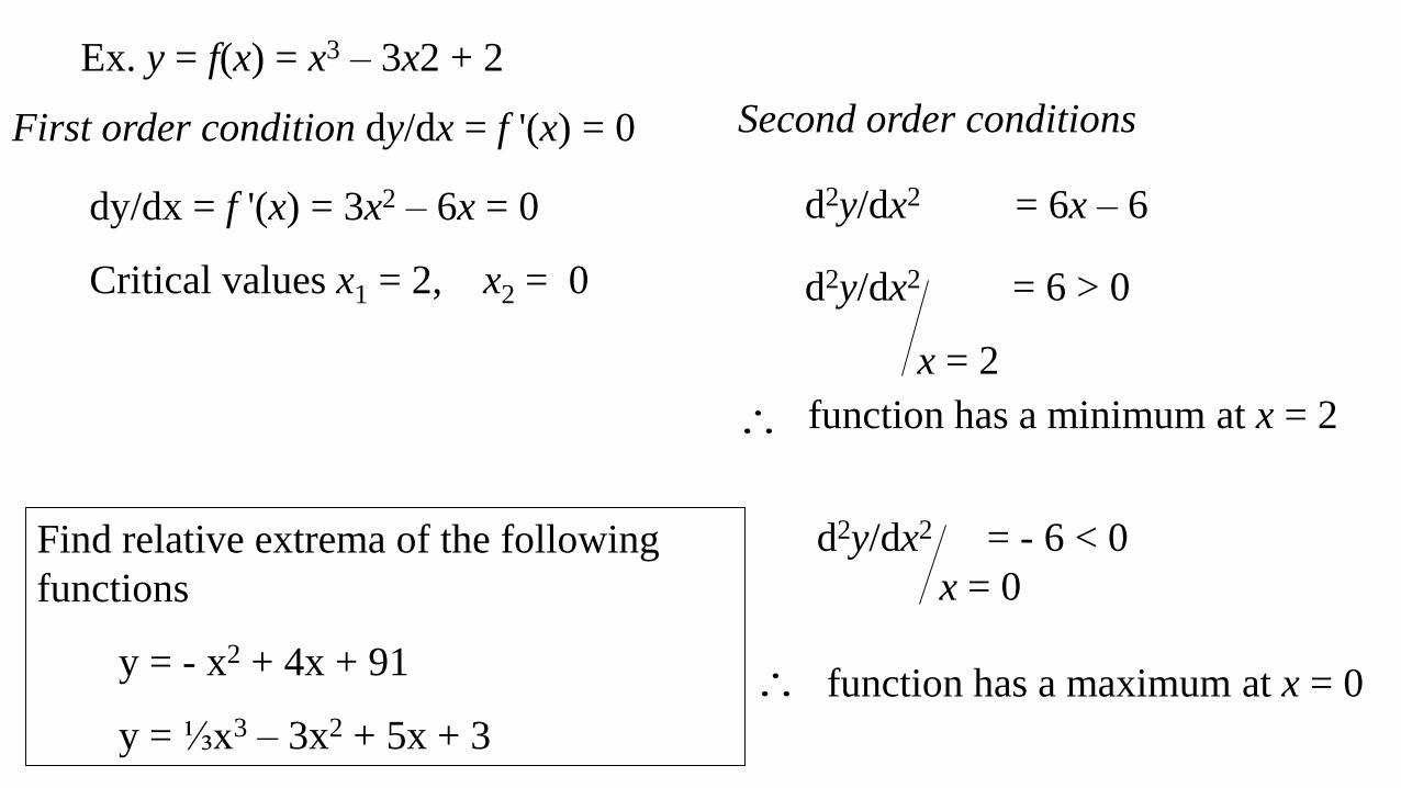
Ex. y = f(x) = x3 – 3x2 + 2
First order condition dy/dx = f '(x) = 0
dy/dx = f '(x) = 3x2 – 6x = 0
Critical values x1 = 2, x2 = 0
Second order conditions
d2y/dx2 = 6x – 6
d2y/dx2 = 6 > 0
x = 2
function has a minimum at x = 2
d2y/dx2 = - 6 < 0
x = 0
function has a maximum at x = 0
Find relative extrema of the following
functions
y = - x2 + 4x + 91
y = ⅓x3 – 3x2 + 5x + 3

If d2y/dx2 = f ''(x) = 0 ?
fujekz ;;ajhl oZ
(1). x yz w.h x0 g l=vd w.hl izg f,dl= w.hla olajd fjkia jk úg f ''(x)yz
,l=K fjkia jk wdldrh kzrZCIKh l< hq;= h' ta wkqj"
i ,l=K + izg – olajd fjkia fõ kï x0 oZ Y%z;hg we;af;a Wmrzuhlz
ii ,l=K – izg + olajd fjkia fõ kï x0 oZ Y%z;hg we;af;a wjuhlz
iii ,l=K fjkia fkdfõ kï x0 k;zjr\;k ,CIHhlz'
First order condition dy/dx = f '(x) = 0
dy/dx = f '(x) = 5x4 – 10x3 = 0
5x3 (x -2) = 0
wjê w.h x = 0, x = 2
172
5)( 45 xxxfyExample

Second order condition
d2y/dx2 = 20x3 – 30x2 = 0
d2y/dx2 = 160 – 120 = 40 > 0
x = 2
x = 2 oZ Y%z;hg we;af;a wjuhlz‘
wju w.h f(2) = 32 – 40 + 17 = 9
d2y/dx2 = 0
x = 0
i. x0 oZ Y%z;hg we;af;a Wmrzuhla o wjuhla o kzYaph lzrZug f '(x) g -1 yd +1 wdfoaY lr
,l=K fjkia jk wdldrh kzrZCIKh l< hq;= h'
dy/dx = 15 x = - 1
dy/dx = - 15
x = 1
jHq;amkakfha ,l=K Ok isg RKg udre jk kzid x0 oZ Y%z;hg we;af;a Wmrzuhlz'

ii. by< >Kfha jHq;amkak .ekZu
- tf,i ,efnk m<uq jk Y+kH fkdjk by< >Kfha jHq;amkakhg x = x0 wdfoaY lrkak'
- ,efnk w.h T;af;a kï x0 k;zjr\;k ,CIHhlz‘
- brÜg w.hla kï x0 w;Hka; ,CIHhlz'
- Ok brÜg w.hla kï wjuhlz'
- RK brÜg w.hla kï Wmrzuhlz'
by; WodyrKh d2y/dx2 = 20x3 – 30x2
d2y/dx2 = 0
x = 0
d3y/dx3 = 60x2 – 60x
d3y/dx3 = 0
x = 0
d4x/dx4 = 120x - 60
d4x/dx4 = - 60 < 0
x = 0
w.h brgAg kzid x = 0 w;Hka; ,CIHhlz' th
RK kzid x =0 oZ Y%z;hg we;af;a Wmrzuhlz'

Extreme Values of a Function of Two Variables
Condition Maximum Minimum
First order or
Sufficient
fx = fy = 0 fx = fy = 0
Second order or
Necessary
fxx, fyy < 0
and
fxx fyy >
fxx, fyy > 0
and
fxx fyy >
z = f(x, y)
2xyf 2
xyf

1. The total cost of producing a given commodity is
TC = ¼ x2 + 30x + 25 and the price of the commodity is
P = 60 - ½ x.
Find the level of output which yield the maximum profit
2. Cost function of a perfectly competitive firm is
TC = 1/3 q3 – 5q2 + 30q + 10
If price p = 6, find the profit maximizing output level.

For second order condition
fxx = 48x – 6 fyy = 2 fxy = 2 fyx = 2
When x = 0
fxx = - 6 fyy = 2
• Since the signs of fxx and fyy are opposite, the product of them yield a
negative value. Obviously it is less than , hence failed the second
order condition.
• Opposite signs of fxx and fyy suggests that the function has a saddle
point at x = 0.
When x = 1/3
fxx = 10 fyy = 2 fxy = 2
The product of fxx and fyy > f 2xy , second order condition satisfies for a
minimum. Point x = 1/3 and y = -1/3 is a minimum and minimum value
of the function is 23/27.
2xyf

eg. Find the extreme value(s) of z = 8x3 + 2xy – 3x2 + y2 + 1
First order condition is fx = 0 and fy = 0
fx = ∂z/∂x = 24x4 + 2y – 6x = 0
fy = ∂z/∂x = 2x + 2y = 0
(1)
(2)
From (2) y = - x
Substituting into (1) 24x2 – 8x = 0
3x2 – x = 0
x(3x – 1) = 0
x1 = ⅓, y1 = - ⅓
x2 = 0 y2 = 0

Economic applications
Profit maximization
Profit (Π) = Total Revenue (R) – Total Cost (C)
Π = R – C
R = f(q) and C = f(q)
Π (q) = R(q) – C(q)
For profit maximization, the difference between R(q) and
C(q) should be maximized.
First order condition
dΠ/dq = Π' = 0

Π' (q) = R'(q) – C'(q)
= 0 iff R'(q) = C'(q)
Thus, at the output level which yield maximum profit,
R'(q) = C'(q)
MR = MC
This is the first order condition for profit maximization.

Second order conditiond2Π/dq2 = Π''(q) < 0
Π''(q) = R''(q) - C''(q)
< 0 iff R''(q) < C''(q)
Thus, to satisfy the second order condition R''(q) < C''(q).
R''(q) = the rate of change of MR
C''(q) – the rate of change of MC
At the output level which MC = MR, and R''(q) < C''(q)
profit is maximized.

The demand and cost functions of a firm is given respectively
as P = 32 – Q and C = 21Q + 24.
i. Find the output level that maximize the total revenue (TR).
ii. Find the output level that maximize the profit (Π).

The profit function of a firm is given as
503983
1 23 qqq
Find the output level that maximize the profit.

2. The total cost of producing a given commodity is
TC = ¼ x2 + 35x + 25 and the price of the commodity is P = 50 - ½ x.
i. Find the level of output which yield the maximum profit
ii. Show that average cost is minimum at this output level.
3. Cost function of a perfectly competitive firm is TC = 1/3 q3 – 5q2 + 30q + 10
If price p = 6, find the profit maximizing output level.
1. Determine maxima and/or minima of the following function:
503983
1 23 qqqy
4. For a new product, a manufacturer spends Rs. 100,000 on the infrastructure
and the variable cost is estimated as Rs.150 per unit of the product. The sale
price per unit was fixed at Rs.200. Find the break-even point.

5. A manufacturing company finds that the daily cost of producing x items of a
product is given by C(x) = 210x+7000.
(i) If each item is sold for Rs. 350, find the minimum number that must be
produced and sold daily to ensure no loss.
(ii) If the selling price is increased by Rs. 35 per piece, what would be the
break-even point?
6. The cost function for x units of a product produced and sold by a company is
C(x)=2500+0.005x2 and the total revenue is given as R = 4x. Find how many
items should be produced to maximize the profit. What is the maximum profit?
7. If the total cost function C of a product is given by 75
72
x
xxC
Prove that the marginal cost falls continuously as the output increases.

8' Total cost function of a firm is given as Find the
output level that minimize total cost (TC).
22145.43
1 23 qqqTC
90505.83
1 23 qqqTC
9. Total cost function and demand functions of a firm respectively are
and 22-0.5q-P = 0'
Find the output level that maximize the total revenue (TR) and the profit (Π).
10. Short production function of a firm is Q = 6L2-0.4L3
Q is the output and L is labor input.
i. Find average product (AP) and marginal product (MP) of labor input.
ii. Find the quantity of labor which maximize output'
iii. Find the level of output which maximize average product of labor.

11. A Company produced a product with Rs 18000 as fixed costs.
The variable cost is estimated to be 30% of the total revenue when it is sold at a
rate of Rs.20 per unit. Find the total revenue, total cost and profit functions.
12. The total revenue received from the sale of x units of a product is given by
R(x) = 12x +2x2+ 6.
Find (i) the average revenue
(ii) the marginal revenue
(iii) marginal revenue at x = 50
(iv) the actual revenue from selling 51st item