Sandia National Laboratories is a multi-program laboratory managed and operated by Sandia Corporation,!wholly owned subsidiary of Lockheed Martin Corporation, for the U.S. Department of Energyʼs!

National Nuclear Security Administration under contract DE-AC04-94AL85000.!

Mathematical Programming and Combinatorial Heuristics

Cynthia Phillips Sandia National Laboratories

caphill@sandia.gov March 18, 2011

Slide 2

Mixed Integer programming (IP)

Min Subject to:

• Can also have inequalities in either direction (slack variables):

•  Integer variables represent decisions (1 = yes, 0 = no) • Surprisingly expressive • Many good commercial and free IP solvers

cTx

aiTx ! bi " ai

T x + si = bi , si # 0!

!

Ax " b! " x " ux = (xI , xC )xI # Z n (integer values)xC # Q $ n (rational values)

Slide 3

Terminology: Mathematical Programming

In this context programming means making decisions. Leading terms say what kind: •  (Pure) Integer programming: all integer decisions • Linear programming • Quadratic programming: quadratic objective function • Nonlinear programming: nonlinear constraints • Stochastic programming: finite probability distribution of scenarios

Came from operations research (practical optimization discipline)

Computer programming (by someone) is required to solve these.

Slide 4

Sensor Placement = p-median

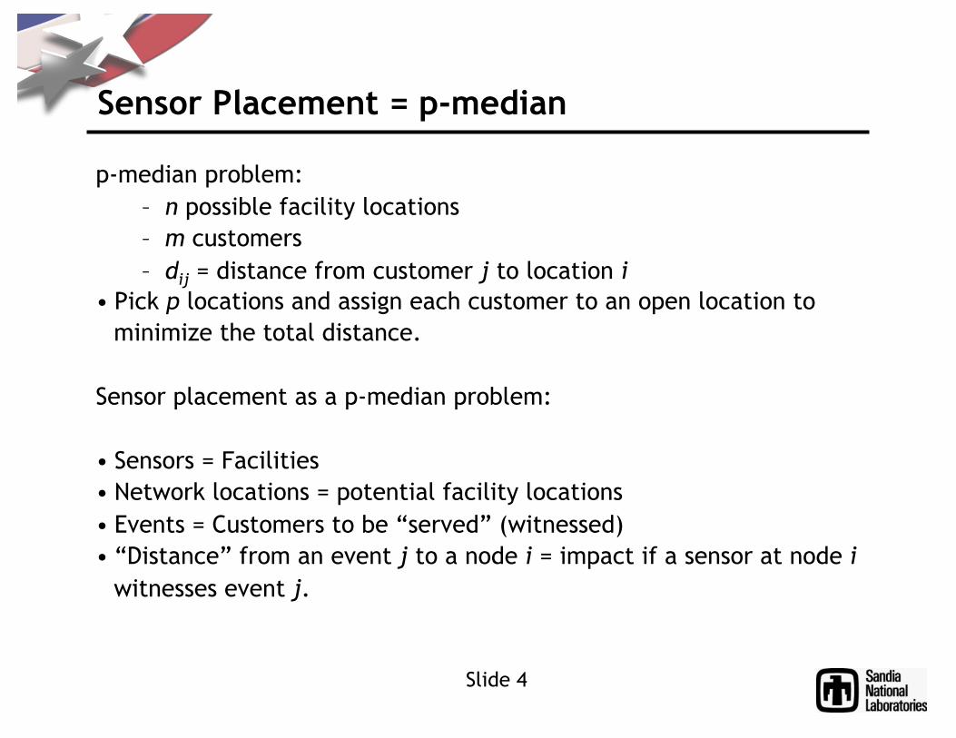
p-median problem: –  n possible facility locations –  m customers –  dij = distance from customer j to location i

• Pick p locations and assign each customer to an open location to minimize the total distance.

Sensor placement as a p-median problem:

• Sensors = Facilities • Network locations = potential facility locations • Events = Customers to be “served” (witnessed) • “Distance” from an event j to a node i = impact if a sensor at node i

witnesses event j.

Slide 5

Sensor Placement Mixed Integer Program

!

minimize " jwij xiji#L j$j#A$

s.t.

xij =1i#L j

$ %j # A (every event witnessed)

xij & yi %j # A,i # L j (need sensor to witness)

yii#L$ & p (sensor count limit)

yi # 0,1{ }0 & xij &1

Slide 6

Branch and Bound

Branch and Bound is an intelligent (enumerative) search procedure for discrete optimization problems.

Requires 3 (problem-specific) procedures: • Compute a lower bound (assuming min) b(X)

• Find a candidate solution

–  Can fail

–  Require that it recognizes feasibility if X has only one point • Split a feasible region (e.g. over parameter/decision space)

!

minx"X f (x)

!

"x # X, b(X) $ f (x)

!

x " X

Slide 7

Linear programming (LP) Relaxation

Min Subject to:

• LP can be solved efficiently in theory and in practice

• Relaxation because we’re removing constraints –  All feasible IP solutions are LP feasible –  Best LP solution is a lower bound on best IP solution

cTx

!

!

Ax " b! " x " ux = (xI , xC )xI # Z n (integer values)xC # Q $ n (rational values)

Slide 8

Solution Strategy: Branch-and-Bound

•  Incumbent is best feasible solution found so far • Need incumbent to prune • Best first expansion (sometimes depth first till incumbent) • LP Relaxation for lower bound • Lowest lower bound in open nodes (frontier) gives gap • “Gradients” to select branching variable.

x j = 1 x j = 0 x k = 0 x k = 1

x i = 0 x i = 1

Root = original problem

fathomed infeasible

terminal

Slide 9

Linear Programming Geometry

The solutions to a single inequality form a half space (in n-dimensional space)

!

aT x " b, x # Qn

!

aT x = b

feasible

Slide 10

Linear Programming Geometry

Intersection of all the linear (in)equalities form a convex polytope • Can be unbounded • Optimal at extreme point (corner or face)

feasible

Objective family

cT x = b1

cT x = b2

Slide 11

IP Geometry

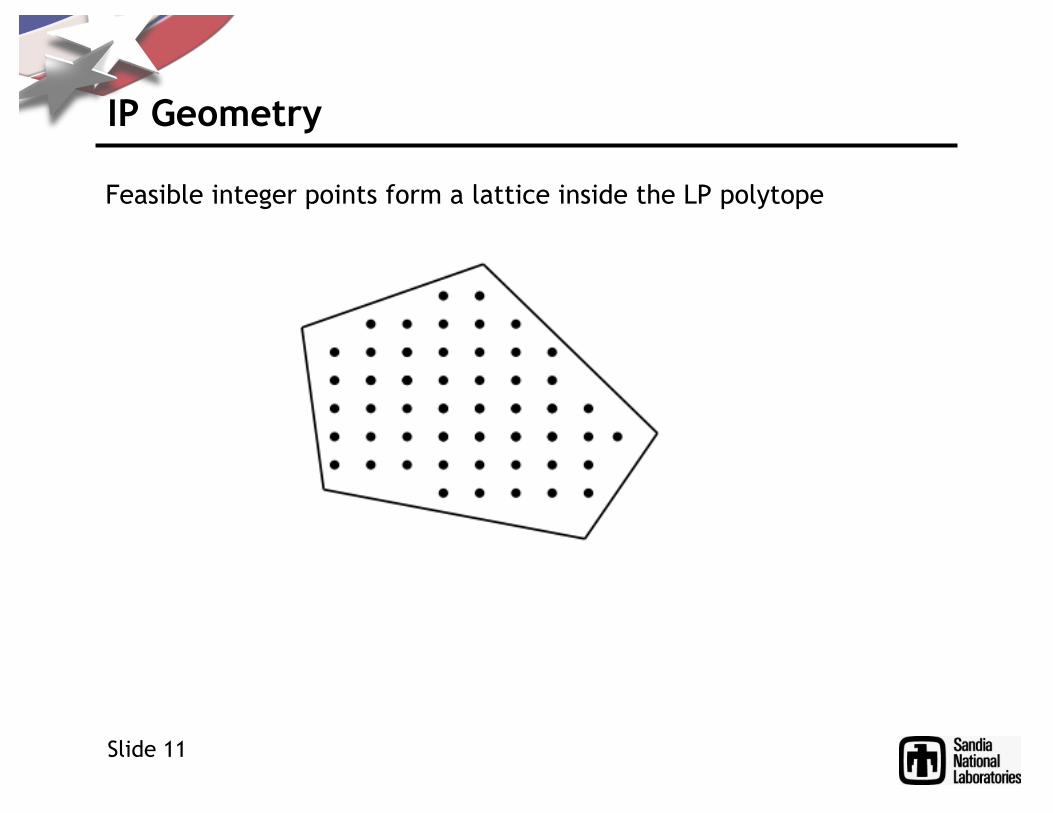
Feasible integer points form a lattice inside the LP polytope

Slide 12

IP Geometry

The convex hull of this lattice forms the integer polytope • Can have an exponential number of faces

Slide 13

IP/LP Geometry

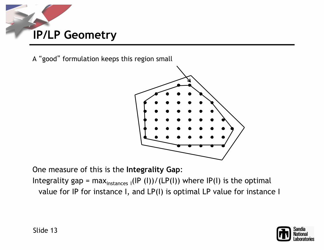
A “good” formulation keeps this region small

One measure of this is the Integrality Gap: Integrality gap = maxinstances I(IP (I))/(LP(I)) where IP(I) is the optimal

value for IP for instance I, and LP(I) is optimal LP value for instance I

Slide 14

Strengthen Linear Program with Cutting Planes

Original LP Feasible region

LP optimal solution

Cutting plane (valid inequality)

Integer optimal • Make LP polytope closer to integer polytope • Apply before branching to control exponential growth • General classes, or problem-specific • Can use families of constraints too large to explicitly list

–  Exponential, pseudopolynomial, polynomial (n4, n5)

Slide 15

Redundant Constraints

• At the optimal point for a linear program, some constraints can be nonbinding (non-tight, redundant)

Slide 16

Separation for Linear Programming

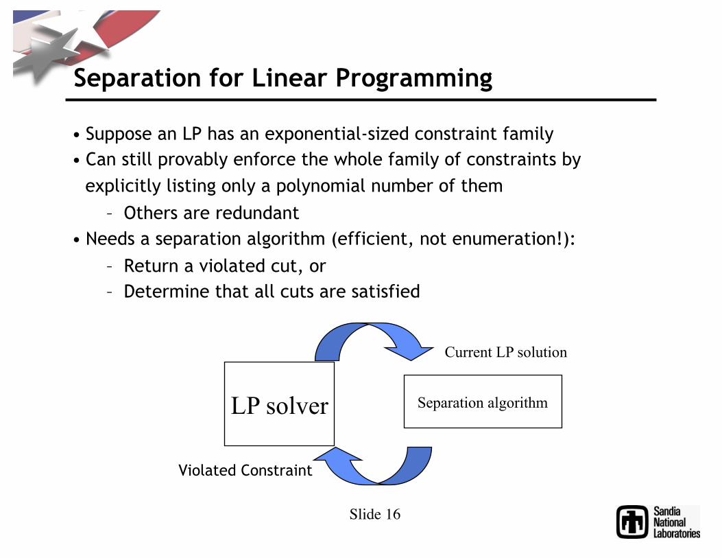
• Suppose an LP has an exponential-sized constraint family • Can still provably enforce the whole family of constraints by

explicitly listing only a polynomial number of them –  Others are redundant

• Needs a separation algorithm (efficient, not enumeration!): –  Return a violated cut, or –  Determine that all cuts are satisfied

LP solver Separation algorithm

Current LP solution

Violated Constraint

Example: Traveling Salesman Problem

Slide 17

min cij! xij

• Subject to: xiji! = 2 "j

xij # 0,1{ }

Disconnected subtours

Should have at least 2 edges between each Partition of nodes

Example: Traveling Salesman Problem

Slide 18

min cij! xij

• Subject to: xiji! = 2 "j

xij # 0,1{ }

Disconnected subtours

Separate with min cut (efficient) using the LP values. Ensure the minimal (fractional) cut is at least 2.

S S

If LP for relaxation edge weights xij*

for this cut < 2, add subtour elimination contraint:

xij(i, j )!Ei!S, j!S

" # 2

Slide 19

Value of a Good Feasible Solution Found Early

•  Simulate seeding with optimal (computation is a proof of optimality) • Good approximations for stopping early

x k = 0 x k = 1

x i = 1

x j = 1 x j = 0

x i = 0

Root Problem = original

fathomed infeasible

Slide 20

Linear Programming (LP) Relaxation-Based Approximation

• Variables can take rational values (relax integrality constraints) • Efficiently solvable: gives lower bound on optimal IP solution • Common technique:

–  Use structural information from LP solution to find feasible IP solution

–  Bound quality using LP bound •  Integrality gap = (best IP solution)/(best LP solution) • This technique cannot prove anything better than integrality gap

Slide 21

Example: Vertex Cover

Find a minimum-size set of vertices such that each edge has at least one endpoint in the set.

2

1 4

7

5 3

6

Slide 22

Example: Vertex Cover

2

1 4

7

5 3

6

vi =1 if vertex i is in the VC0 otherwise ! " #

min vi!s.t. vi + v j " 1 # i, j( )$E vi $ 0,1{ }

Slide 23

2-Approximation algorithm for Vertex Cover

• Solve the LP relaxation for vertex cover:

• Select all vertices i such that vi ≥ 1/2. • This covers all edges: at least one endpoint will have value at least

1/2. • Each such vertex contributed as least 1/2 to the optimal LP

solution, so rounding to 1 at most doubles cost.

min vi!s.t. vi + v j " 1 # i, j( )$E 0 % vi % 1

Problem-Specific Heuristics

• LP-based optimization –  Lot’s of examples including scheduling, network design

• Other non-LP-based problem-specific approximations that come with quality guarantees, especially:

–  Graph algorithms –  String algorithms –  Scheduling

See for example Cresenzi and Kann “A Compendium of NP Optimization problems: http://www.csc.kth.se/~viggo/wwwcompendium/

Slide 24

Slide 25

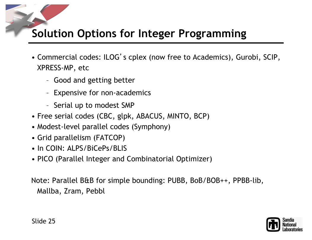
Solution Options for Integer Programming

• Commercial codes: ILOG’s cplex (now free to Academics), Gurobi, SCIP, XPRESS-MP, etc

–  Good and getting better

–  Expensive for non-academics

–  Serial up to modest SMP • Free serial codes (CBC, glpk, ABACUS, MINTO, BCP) • Modest-level parallel codes (Symphony) • Grid parallelism (FATCOP) •  In COIN: ALPS/BiCePs/BLIS • PICO (Parallel Integer and Combinatorial Optimizer) Note: Parallel B&B for simple bounding: PUBB, BoB/BOB++, PPBB-lib,

Mallba, Zram, Pebbl

Algebraic Modeling Languages

• Let’s you think like this: Min Subject to: • Translates the algebra (parameters, variables, constraints, objective)

into matrix, flat variable vector, etc, that solvers require • Nice compromise between algebra and computer language

Slide 26

cTx

!

Ax " b! " x " ux = (xI , xC )xI # Z n (integer values)xC # Q $ n (rational values)

Algebraic Modeling Languages

• Commercial: AMPL, AIMMS, GAMS, LINDO, MAXIMAL, Mosel, OPL, TOMLAB

• Free: FlopC++, APLEpy, CVXOPT, PuLP, POAMS, OpenOpt, NLPy, PYOMO

–  FlopC++ (e.g.) is more tightly coupled • Use a low-level programming language • Directly apply MILP solvers using language extensions

–  AMPL (e.g.) more loosely coupled • Use a high-level programming language • Generate a generic problem representation • Apply an externally defined solver

–  Pyomo gives the full power of python for customization

Slide 27

Slide 28

Multiple Objectives Revisited

Min Subject to:

!

Ax ! b! ! x ! ux = (xI , xC )xI " Zn (integer values)xC "Q

#n (rational values)

c1T x

c2T x

Slide 29

Multiple Objectives Revisited

Min Subject to:

!

Ax ! b

c2T x ! B2

! ! x ! ux = (xI , xC )xI " Zn (integer values)xC "Q

#n (rational values)

c1T x

c2T x

Slide 30

Multiple Objectives Revisited

Min Subject to:

!

Ax ! b! ! x ! ux = (xI , xC )xI " Zn (integer values)xC "Q

#n (rational values)

w1c1T x +w2c2

T x

Pareto Front

• Pareto Front can be non-convex

Slide 31

c1Tx

c2Tx

Pareto Front

• Weighted objectives only find points on the convex hull of the pareto front

Slide 32

c1Tx

c2Tx

w1c1Tx + w2c2

Tx = b1

w1c1Tx + w2c2

Tx = b2

Custom Branch and Bound

Example from last time: Protein-Peptide Docking • Amino acid sequence fixed • Backbone rigid • Pick a rotomer (3d shape) for each sidechain • Design version pick amino acids too • Minimize energy (rotamer-protein, rotamer-rotamer)

Slide 33

A1 A1 A2 A3

R13

R12

R11

R13

R12

R11

R22

R21

R31

Slide 34

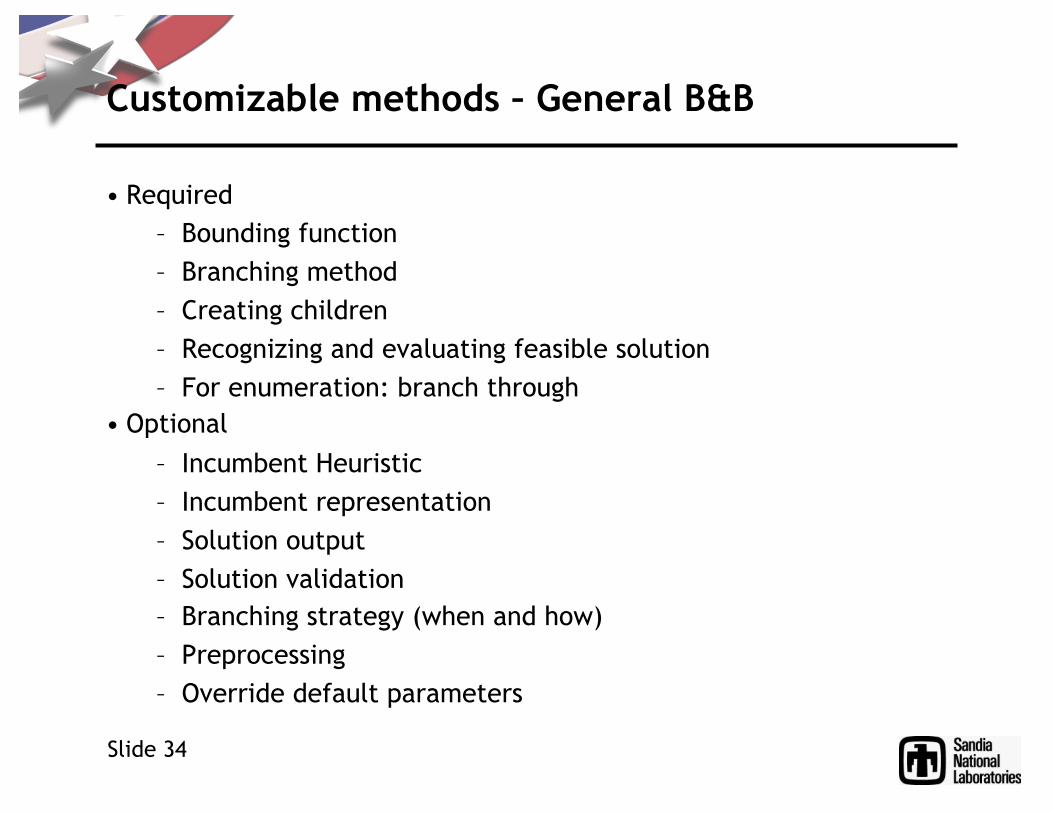
Customizable methods – General B&B

• Required –  Bounding function –  Branching method –  Creating children –  Recognizing and evaluating feasible solution –  For enumeration: branch through

• Optional –  Incumbent Heuristic –  Incumbent representation –  Solution output –  Solution validation –  Branching strategy (when and how) –  Preprocessing –  Override default parameters

Slide 35

Protein-Peptide Docking: Bounding

Apply combinatorial optimization methods developed for side chain prediction (Canutescu et al. ’03)

–  Simple bound:

This bound must respect branching decisions

–  Some rotamers are forced –  Some rotamers are disallowed

• Complication not mentioned last time: some pairs of rotamer choices for different sidechains are not feasible

minr Eiri! + minr,s:(i,r, j,s)"X

i< j! Airjs

Slide 36

Protein-Peptide Docking: Branching

• Pick a location on the chain to branch on –  Initially just one that hasn’t been tried before –  Keep track of bound changes, subsequently pick an undecided

sidechain with best gradient

• To branch, put half of the remaining possibilities in each child –  Usually stored sorted –  Can just split list –  Round robin for better balance

Protein-Peptide Docking: Incumbent Heuristic

• Pick a starting point: –  Deterministically start with rotamer at each site with lowest

rotamer-protein energy • Go greedily in order based on feasibility

–  Random, biased by rotamer-protein energy •  Iterative Improvement

–  Heuristically start with sidechain location with fewest options –  Starting with lowest energy (with protein) romater, try to find

an improving swap • Measured based on total energy, which includes rotamer-

rotamer interactions

Slide 37

Slide 38

All PICO’s parallelism comes (almost) for free

User must • Define serial application • Describe how to pack/unpack data (using a generic packing tool) C++ inheritance gives parallel management Be careful of ramp up!

Wasted processors vs creation of unnecessary work that can lead to slowdown

PICO parallel MIP Serial MIP application

Parallel MIP application

Enumeration (cont’d)

Implementation with PEBBL: –  Leverage MPI-based parallelization in PEBBL –  Parallelized enumeration with distributed cache

Slide 39

Metaheuristics

• Gross strategies for controlling local search –  Steepest Descent –  GRASP –  Evolutionary algorithms –  Simulated Annealing –  Tabu Search –  Ant Colony –  Etc

Slide 40

Neighborhood

• Key concept: making a move to a “neighboring” solution • Examples:

–  Sensor placement problem: move one sensor to a new location –  Protein-peptide docking: replace a rotamer with another –  Spanning tree: add an edge and remove another on the cycle

it creates

•  Neighborhoods can be very large, requiring efficient algorithms just to compute a move.

Slide 41

X

Steepest Descent

• Always move to the neighbor that improves the objective function the most.

–  Reaches local optimum with respect to neighborhood

• Good idea to run this on all solutions found heuristically –  LP-based approximations –  Other algorithms with provable approximation bounds

Slide 42

Slide 43

Sensor Placement Heuristic Solvers • GRASP: Greedy Randomized Adaptive Search Procedures

–  Start with many randomized points, picked by building a solution with a greedy bias

• Example: Add sensors one at a time, biased exponentially based on impact reduction

–  Do steepest descent (or other local search) from each point

•  Move one senor

–  Take best seen

•  Much faster than IP (10x) Curious structure: Almost always optimal

–  Even with just one iteration of start + descent

–  If not optimal, very close •  WHY?

Genetic Algorithms

• Start with a population of feasible solutions (e.g. random) • The most fit (best objectives) survive • Solutions reproduce by

–  Mutation (random local changes) –  Crossover (merging of two current solutions)

• Example: protein-peptide docking –  Mutation: Swap one or more rotamers –  Crossover (can be at any consistent point on backbone)

• Infeasible combinations die

Slide 44

A Birds Eye View of GO Slide 45

GA Special Case of Population Search

•  Idea: •  Maintain a set/population of points in each iteration •  Generate new points with

–  Local steps about points –  Recombination steps using two or more ‘parents’

•  Keep the ‘best’ points seen so far

•  Scatter Search: •  A general population-based meta-heuristic •  Exploits interplay between diversification and intensification

–  Intensification through •  local improvement, •  directed recombination, and •  use of a reference set of best points generated

–  Diversification through methods that introduce systematic variation

A Birds Eye View of GO Slide 46

Population Search

•  Differential Evolution/Controlled Random Search: •  Optimizes on reals •  Only keep new points if they are improving •  Recombination operators:

–  Differential Evolution

–  Controlled Random Search x

For Some indices (below random) Combine with 3 Other random pts

Simulated Annealing

• From current point, pick a random neighbor •  If random neighbor is an improvement, make the move •  If it is not, take the move anyway with some probability

–  Jump out of local min –  Mixture starts out “hot” with a higher probability of jumping –  Over time it “cools” to anneal to a local min

Slide 47

Tabu Search

•  Philosophy: to derive and exploit a collection of principles of intelligent problem solving.

•  Idea: use flexible memory to create and exploit structures for taking advantage of history

•  TS data structures try to incorporate four dimensions of search history: recency, frequency, quality, and influence

–  For example, avoid tracking back over recently searched space

Slide 48

Ant Colony Optimization

• Motivated by ant foraging strategy –  Easiest to understand with path examples –  For example, local agents

• Find good solution at random, leaving pheromone • Other ants follow/reinforce pheromone trail • Pheromone evaporates so shortest paths are favored

Slide 49

(wikipedia)

A Birds Eye View of GO Slide 50

A Categorization

Method Heuristic Randomized Exact Discrete Continuous Constraints

B&B X X X X

DIRECT X X X

Scatter Search X ? X X X

DE/CRS X ? X

EAs X X X X X

Response Surface X X X

Multistart LS X X X X

GRASP X X X ? X

Cluster LS X ? X X

Continuation X X X

Tunneling X X X

Tabu Search X ? X ? X

Simulated Annealing X X X X ?

Ant Colony X X X

(Courtesy: Bill Hart)

Metaheuristics Libraries (Frameworks)

•  jMetal (*), HeuristicLab, EasyLocal, Paradiseo (*), CodeA (Nottingham), MALLBA, Coopr

Where (*) possibly most popular. Matlab and Excel have GAs, etc Woodruff to Voβ: “I’m making a class library” Voβ replies: “That’s nice, but no one will use it. Years later… Voβ to Woodruff: “We’re making a class library” Woodruff : “That’s nice, but no one will use it. [Thanks to Dave Woodruff, UC Davis]

Slide 51

Writing metaheuristics

• People tend to “roll their own” –  Have to write the procedures anyway –  Don’t have to learn a library interface

• That said, for things like GAs, it makes sense to use the knowledge of the meta-process from years of research and experimentation (e.g. in Coopr)

Slide 52

Non-linear programming Solvers

• There are some nonlinear programming solvers –  SNOPT, BARON –  Might only give local optima in general

• Mixed-Integer nonlinear programming –  BONMIN, Couenne, Minotaur –  These generally do branch-and-bound, solving non-linear

subproblems

Slide 53

Slide 54

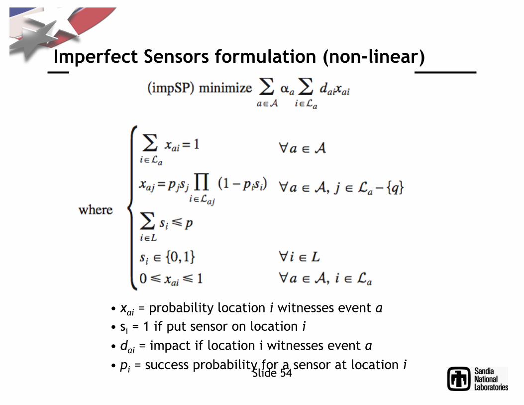
Imperfect Sensors formulation (non-linear)

• xai = probability location i witnesses event a • si = 1 if put sensor on location i • dai = impact if location i witnesses event a • pi = success probability for a sensor at location i

Slide 55

Methods we considered for solving impSP

•  Ignore imperfection • Exact linear integer program based on zones • Nonlinear solver (fractional) • Local search with imperfect-sensor objective • Random Sampling • One-imperfect witness

11,575 nodes 9705 events 40 sensors

For Combinatorial Problems

• Different performance guarantees –  Optimal (or proven gap), provable approximation, none

• Tradeoff between search time and quality •  If your problem

–  is an integer program –  You need a really good solution –  Maybe you are only going to ask once

Then IP solvers and math programming languages are good enough to just code up an IP quickly and try it •  If you

–  have the time –  Have to run lots of times and want something super fast

it is usually worth doing something custom, even if heuristic, and benchmarking vs the optimal if possible.

Slide 56