MATHEMATICAL MODELS OF BRAIN DEFORMATION …isml.ecm.uwa.edu.au/ISML/images/0/0e/Isml-no-01-2006.pdf · MATHEMATICAL MODELS OF BRAIN DEFORMATION BEHAVIOUR FOR COMPUTER ... This Report

Research Report of Intelligent Systems for Medicine Laboratory

Report # ISML/01/2006, February 2006

MATHEMATICAL MODELS OF BRAIN

DEFORMATION BEHAVIOUR FOR

COMPUTER-INTEGRATED NEUROSURGERY

K. Miller, Z. Taylor, A. Wittek Intelligent Systems for Medicine Laboratory School of Mechanical Engineering The University of Western Australia 35 Stirling Highway Crawley WA 6009, AUSTRALIA Phone: + (61) 8 6488 7323 Fax: + (61) 8 6488 1024 Email: [email protected] http://www.mech.uwa.edu.au/~kmiller/ http://www.mech.uwa.edu.au/ISML/

mailto:[email protected]

http://www.mech.uwa.edu.au/~kmiller/

http://www.mech.uwa.edu.au/ISML/

Research Report # ISML/01/2006 K.Miller, Z.Taylor, A.Wittek

Contents 1 Introduction ----------------------------------------------------------------------- 3 2 Engineering modelling process ---------------------------------------------- 3 3 System for computing brain deformations -------------------------------- 6 4 Mechanical properties of brain tissue -------------------------------------- 7 5 Applications ----------------------------------------------------------------------- 10 5.1 Modelling the brain for neurosurgical simulation ------------------- 10

5.1.1 Linear versus finite deformation elasticity ---------------- 10 5.1.2 Example of fully non-linear computation of brain deformation and reaction forces ----------------------------------- 11

5.2 Modelling the brain for image registration --------------------------- 16 5.3 Modelling the brain for prognosis of structural diseases -------- 20 5.4 Computer simulation of the effects of the tumor growth -------- 22

6 Conclusions ---------------------------------------------------------------------- 23 Glossary of technical terms ----------------------------------------------------------- 25 References -------------------------------------------------------------------------------- 27

Abstract This Report discusses mathematical models of brain deformation behaviour for neurosurgical simulation, brain image registration and computer simulation of development of structural brain diseases. These processes can be reasonably described in purely mechanical terms, such as displacements (or displacement field), internal forces (stresses), pressure (or pressure field), flow and velocity of the flow, etc, and therefore they can be analysed using established methods of continuum mechanics. We advocate the use of fully non-linear theory of continuum mechanics. Partial differential equations (PDE’s) of this theory, in most practical cases, cannot be solved analytically, however an approximate numerical solution can be calculated on a computer. We recommend the choice of non-linear (i.e. allowing finite deformation) finite element procedures as an effective and proven numerical method for solving the PDE’s of continuum mechanics. The mechanical response of brain tissue to external loading is characterised by a non-linear stress-strain relationship and a non-linear stress – strain rate relationship. Moreover, the brain is much stiffer in compression than in tension. We show how these experimentally measured properties can be taken into account when choosing a constitutive model of the brain tissue for a particular application. We support our recommendations and conclusions with four examples: computation of the reaction force acting on a surgical tool, computation of the brain shift for image registration, simulation of the development of hydrocephalus, and simulation of the effects of tumour growth.

Key words: brain, biomechanics, computational radiology, surgical simulation, structural disease simulation

2


1 Introduction Mathematical modelling and computer simulation have proved tremendously successful in engineering. Computational mechanics has enabled technological developments in virtually every area of our lives. One of the greatest challenges for mechanists is to extend the success of computational mechanics to fields outside traditional engineering, in particular to biology, biomedical sciences, and medicine (52). By extending the surgeons' ability to plan and carry out surgical interventions more accurately and with less trauma, Computer-Integrated Surgery (CIS) systems could help to improve clinical outcomes and the efficiency of health care delivery. CIS systems could have a similar impact on surgery to that long since realised in Computer-Integrated Manufacturing (CIM). In computational sciences, the most critical step in the solution of the problem is the selection of the physical and mathematical model of the phenomenon to be investigated. Model selection is most often a heuristic process, based on the analyst’s judgment and experience. Often, model selection is a subjective endeavour; different modellers may choose different models to describe the same reality. Nevertheless, the selection of the model is the single most important step in obtaining valid computer simulations of an investigated reality (52).

In this paper we present how various aspects of computer-integrated neurosurgery can benefit from the application of methods of computational mechanics. We discuss physical and mathematical models of the brain deformation behaviour developed in the Intelligent Systems for Medicine Laboratory at The University of Western Australia. We chose to focus on the following application areas:

1. Neurosurgical simulation for operation planning and surgeon training; 2. Neuroimage analysis (computational radiology); 3. Simulation of the development of structural diseases for prognosis and diagnosis.

Following the Introduction (Section 1), in Section 2 we describe a standard procedure of creating computational models of real phenomena: the engineering modelling process. In Section 3, a conceptual framework for the system for computing brain deformations is discussed. Section 4 presents selected experimental data on the mechanical properties of brain tissue. In Section 5 we consider example applications in areas of surgical simulation, computational radiology and computer simulation of structural diseases of the brain. We conclude with some reflections about the state of the field.

We wrote Sections 1 (Introduction), 2 (Engineering modelling process), 3 (System for computing brain deformations), 6 (Conclusions), and all figures and figure captions for readers without mathematical or engineering background. We also included a glossary of technical terms at the end of the paper (technical terms explained in the Glossary, when used for the first time, appear in the manuscript in italic). Sections 4 (Mechanical properties of brain tissue) and 5 (Applications) are more technical.

2. Engineering modelling process The process of mathematical modelling and computer simulation is presented in Figure 1. Major blocks in the diagram are discussed below.

3


Reality

Physical model

Mathematical model

Numerical model

Numerical solution

Numerical result

QUESTIONS?

In Engineering usually systems of equations + B.C. and I.C.:ODE, DAE, PDF

usually discretisation

usually a sketch

Figure 1. Engineering modelling process

What do we want to know about reality - questions? The most critical element of the modelling process is the clear specification of questions. These questions are related to the desired results of the analysis. Physical model After the questions have been explicitly specified, we may notionally discard many features of reality that we deem irrelevant. This process of simplification leads to a physical model that contains only relevant aspects of reality from the perspective of the specified questions.

For instance, consider that our “reality” is the brain undergoing surgery. Our “questions” clearly depend on the application we have in mind. If our application is a virtual reality neurosurgical simulator, the two most important questions are about the deformation field in the brain, so that it can be displayed for the user, and about reaction forces acting on a surgical tool or surgeon’s fingers, so that a realistic tactile (haptic) feedback can be given to the surgeon. We may safely discard e.g. bio-chemical and electrical aspects of the brain as irrelevant to the problem at hand. To answer questions about deformations and forces it is reasonable to treat the brain in purely mechanical terms, e.g. a reasonable physical model of choice is a single-phase continuum. Mathematical model A mathematical model is created through the selection of equations that describe the physical model. It is important to note that the equations of mechanics do not describe reality but only certain classes of physical models. Therefore it is imperative not to skip the physical modelling stage of the modelling process. A mathematical model describing the brain as a single-phase continuum (the selected physical model) that allows accurate computations of brain’s mechanical response (i.e. finite deformations and internal forces) consists of the

4


differential equations of non-linear continuum mechanics and of a constitutive model capturing the main features of mechanical properties of brain tissue.

However, if our application is the registration of pre- and intra-operative images, we are interested only in deformation fields (and not in forces involved) and therefore the selection of the constitutive model for the brain tissue is of secondary importance (see Section 5.2). It is worth noting that in both cases the use of the equations of linear elasticity would be inappropriate because the assumption of infinitesimal deformations is embedded in them, and therefore they cannot be used to answer questions about finite deformations. Numerical model Mathematical models of computational biomechanics are usually complicated sets of partial differential equations (PDEs) supplemented with boundary and initial conditions. In practice such systems of equations are converted to numerical models (usually through some form of discretisation) and solved using computers. Probably the most effective, and certainly the most popular numerical method for solving such sets of differential equations is the Finite Element Method (3, 79). It is very important to note here that the Finite Element Method is not a modelling method. It is merely a numerical method for solving systems of differential equations – the modelling (i.e. selecting appropriate physical and mathematical models) must be done by an analyst. Assessing the validity of numerical results – feedback loops Because every step in the modelling process is based on assumptions and therefore introduces simplifications, it is necessary to assess the validity of computational results versus the numerical, mathematical and physical model, as well as the reality. This is indicated by “feedback” loops in Figure 1. For example a solution procedure may be unstable and produce an incorrect solution to the numerical model. Or if a computational grid (e.g. a finite element mesh) has not been created correctly, calculated results may be a correct solution to the (incorrect) numerical model, but not to the mathematical model. If equations of the mathematical models were not properly chosen, calculated results may be a correct solution to the numerical and mathematical models but not to the physical model. And finally, if the physical model is not adequate, the numerical results may be a correct solution to the numerical, physical and mathematical models, but may have no relevance to reality.

It is most important to select models that are reliable and effective in predicting the quantities of interest. As it is often difficult to assess the reliability of the model through direct experimentation because the system under investigation either does not exist (e.g. a new fighter jet in the design stage) or conducting experiments on it is difficult or impossible (e.g. the human brain, or many other biological systems), one thinks of a very comprehensive model and measures the response of one’s chosen model against the response of the very comprehensive model. Bathe (3) defines effectiveness and reliability of a model as follows: Effectiveness of a model: The most effective model for the analysis is the one which yields the required response with sufficient accuracy and minimum cost. Reliability of a model: The chosen model is reliable if the required response can be predicted within a specified level of accuracy measured against the response of the very comprehensive model. As very comprehensive models of human organs, including the brain, are rare, the assessment of the reliability of models can be a significant challenge.

5


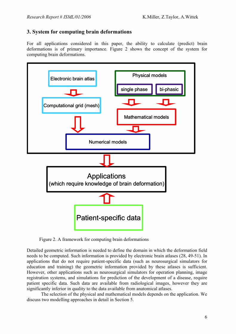
3. System for computing brain deformations

For all applications considered in this paper, the ability to calculate (predict) brain deformations is of primary importance. Figure 2 shows the concept of the system for computing brain deformations.

Electronic brain atlas

Computational grid (mesh)

single phase bi-phasic

Physical models

Numerical models

Applications(which require knowledge of brain deformation)

Patient-specific data

Mathematical models

Electronic brain atlas

Computational grid (mesh)

single phase bi-phasic

Physical models

Numerical models

Applications(which require knowledge of brain deformation)

Patient-specific data

Mathematical models

Figure 2. A framework for computing brain deformations Detailed geometric information is needed to define the domain in which the deformation field needs to be computed. Such information is provided by electronic brain atlases (28, 49-51). In applications that do not require patient-specific data (such as neurosurgical simulators for education and training) the geometric information provided by these atlases is sufficient. However, other applications such as neurosurgical simulators for operation planning, image registration systems, and simulations for prediction of the development of a disease, require patient specific data. Such data are available from radiological images, however they are significantly inferior in quality to the data available from anatomical atlases. The selection of the physical and mathematical models depends on the application. We discuss two modelling approaches in detail in Section 5.

6


A necessary step in the development of the numerical model of the brain is the creation of a computational grid, which in most practical cases is a finite element mesh. The requirements for the mesh type and fidelity depend on the chosen mathematical model and the accuracy of the solution required by the application. Patient-specific data should also include information about mechanical properties of the particular patient’s brain. Average properties, such as those presented in Section 4, may not be sufficient because of the very large variability inherent to biological materials, as clearly demonstrated in the biomechanics literature, see e.g. (7, 38, 42, 56). 4. Mechanical properties of brain tissue Mechanical properties of living tissues form a central subject in biomechanics. In particular, the properties of the muscular−skeletal system, skin, lungs, blood and blood vessels have attracted much attention (see for example (19, 20) and references cited therein). The properties of “very” soft tissues that do not bear mechanical loads (such as brain, liver, kidney, etc.) have not been so thoroughly investigated.

Previous research into the mechanical properties of the brain and brain tissue was motivated by traumatic injury prevention (e.g. (75, 77) and references cited therein) and understanding of structural brain diseases (e.g. hydrocephalus, see (22, 46)). These require investigation into applying a load to brain tissue very quickly and very slowly.

The first papers on the mechanical properties of the brain at moderate loading speeds (relevant to surgical simulation) appeared, to the best of our knowledge, in 1995 (39, 40). Since then, research groups from the University of Sydney (7), University of Pennsylvania (56, 63), Eindhoven University of Technology (10), AIST, Tsukuba, Japan, and The University of Western Australia (41-43) have conducted experiments and presented mathematical models of brain tissue mechanical behaviour. Results obtained by the authors of this contribution and collaborators from AIST, Japan are collected in (38).

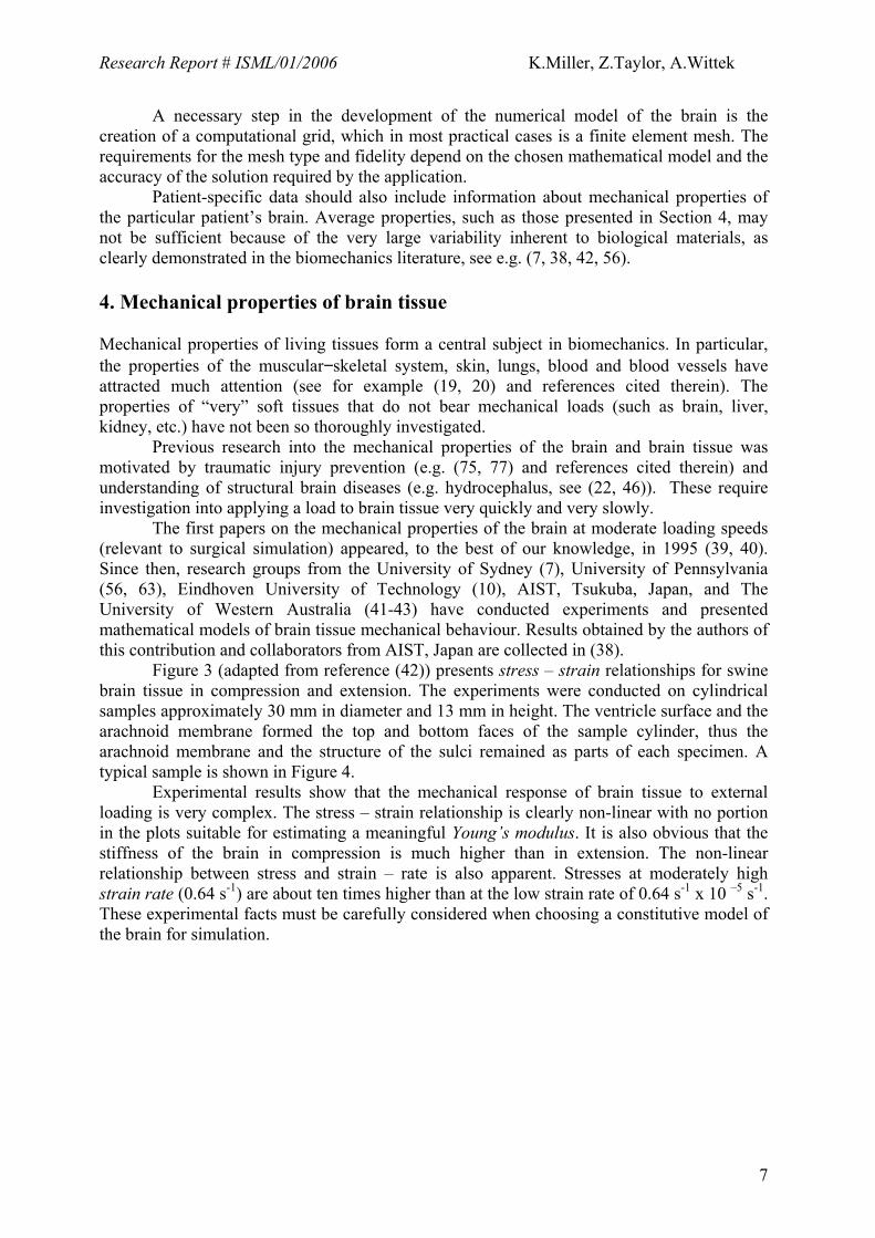
Figure 3 (adapted from reference (42)) presents stress – strain relationships for swine brain tissue in compression and extension. The experiments were conducted on cylindrical samples approximately 30 mm in diameter and 13 mm in height. The ventricle surface and the arachnoid membrane formed the top and bottom faces of the sample cylinder, thus the arachnoid membrane and the structure of the sulci remained as parts of each specimen. A typical sample is shown in Figure 4.

Experimental results show that the mechanical response of brain tissue to external loading is very complex. The stress – strain relationship is clearly non-linear with no portion in the plots suitable for estimating a meaningful Young’s modulus. It is also obvious that the stiffness of the brain in compression is much higher than in extension. The non-linear relationship between stress and strain – rate is also apparent. Stresses at moderately high strain rate (0.64 s-1) are about ten times higher than at the low strain rate of 0.64 s-1 x 10 –5 s-1. These experimental facts must be carefully considered when choosing a constitutive model of the brain for simulation.

7


Figure 3. Experimental (solid line) versus theoretical (dashed line, Equations 1, 2 and Table 1) results for uniaxial compression (41) and extension (42) of brain tissue for various loading velocities. For this simple experimental configuration, Lagrange stress (vertical axis) is the vertical force divided by the undeformed cross-sectional area, and extension (horizontal axis) is the current height divided by the initial height, i.e. extension less than one indicates compression. Negative values of stress indicate compression. a) loading velocity v = 5.0 x 102 mm/min ; corresponding to the strain rate approx. 0.64 s-1. b) loading velocity v = 5.0 mm/min ; corresponding to the strain rate approx. 0.64 s-1 x 10 –2 s-1. c) loading velocity v = 5.0 x 10 –3 mm/min ; corresponding to the strain rate approx. 0.64 s-1 x 10 –5 s-1 (compression only). Note that the stress – strain and stress – strain rate relationships are non-linear, and the stiffness of the brain in compression is much higher than in extension.

8


Figure 4. A typical swine brain tissue specimen used in compression and extension experiments, results of which are given in Figure 3.

To account for such complicated mechanical behaviour we proposed the Ogden-based

hyper-viscoelastic constitutive model of the following form (38, 42):

W =2α 2 [µ(t −τ )

ddτ0

t

∫ (λ1α + λ2

α + λ3α − 3)]dτ (1)

t

µ = µ0[1− gk(1 −k =1

n

∑ e−

τ k )] , (2)

W is the strain energy. λ1, λ2, λ3 (directions 1, 2, 3 correspond to x, y, z) are principal extensions. Their values are 1 for no deformation, greater than 1 for extension and smaller than 1 for compression. α is a material coefficient without physical meaning. We identified the value of α to be –4.7, see Table 1. t and τ denote time. Equation 2 describes viscous response of the tissue. µ0 is the instantaneous shear modulus in the undeformed state. τk are characteristic relaxation times. Stress – strain relationships are obtained by differentiating the energy function W with respect to strains (3, 38). This is analogous to linear elasticity and Hooke’s law. For one-dimensional stretching of the linear elastic material the energy function is:

2

21 εEW = , where E is the Young’s Modulus and ε is the strain. (3)

Stress is computed as the derivative of the energy with respect to strain:

εε

σ EW =∂∂= (4)

Equation 4 is a well-known Hooke’s Law. Because brain’s mechanical response is very complicated Equations 1 and 2 describing the energy function of brain tissue are more complex than Equation 3.

9


The identified from experiment material constants are given in Table 1. One-dimensional response, as predicted by Equations 1 and 2, is shown in Figure 3.

Table 1. List of material constants for the constitutive model of brain tissue,

Equations 1 and 2, n=2 (42). Instantaneous response k=1 k=2

µ0 =842 [Pa]; a=-4.7

characteristic time t1=.5 [s]; g1=0.450;

characteristic time t2=50[s]; g2=0.365;

One advantage of the proposed model is that the constitutive equation presented here

is already available in commercial finite element software (1, 32) and can be used immediately for larger scale computations.

It is very important to examine the simplifying assumptions behind the model

described by Equations 1 and 2, and Table 1: isotropy and incompressibility. 1. Incompressibility.

Very soft tissues are most often assumed to be incompressible (see e.g. (15, 36, 54, 58, 59, 68, 69)). In experiments on brain tissue at moderate strain rates when there is not enough time for significant fluid flow, we have not detected a departure from this assumption.

2. Isotropy (i.e. mechanical properties are assumed to be the same in all directions). Very soft tissues do not bear mechanical loads and do not exhibit directional structure (provided that a large enough sample is considered: for brain we used samples of 30 mm diameter and 13 mm height). Therefore, they may be assumed to be initially isotropic (see e.g. (6, 16, 34, 36, 37, 42, 43, 48, 69)). Prange and Margulies (56) reported anisotropic properties of brain tissue. However, their sample sizes were 1 mm wide. At such a small length scale, the fibrous nature of most tissues will cause detectable difference in directional properties. Experiments discussed here were aimed at identifying “average” properties at the length scale of approx. 1 cm. At such length scales, most very soft tissues can be safely assumed to exhibit no directional variation of mechanical properties. The specimens used in the experiments consisted of the arachnoid membrane, white

matter and grey matter. Subsequently, it could be argued that the experimental results are only valid for such a composite. However, these results are useful in the approximate modelling of the behaviour of brain tissue, which includes spatial averaging of material properties.

5. Applications 5.1 Modelling the brain for neurosurgical simulation The goal of surgical simulation research is to model and simulate deformable materials for applications requiring real-time interaction. Medical applications for this include simulation-based training, skills assessment and operation planning. 5.1.1 Linear versus finite deformation elasticity A neurosurgical simulator must predict the deformation field within the brain, so that it can be displayed to the user, and the internal forces (stresses) so that reaction forces acting on surgical tools can be computed and conveyed to the user through haptic feedback.

10


To allow simulation in near real time, most investigators (with one notable exception (78)), build models based on the simpler equations of linear elasticity. These models are incapable of providing realistic predictions of finite deformations of the tissue, because the infinitesimality of the deformations is assumed. Linearity of the material response is also assumed. Consequently, the principle of superposition holds for linear elastic models, contradicting years of experience accumulated by researchers working on finite deformation elasticity. In the 1970s, when non-linear finite element procedures were under development, many examples of these shortcomings were published, see e.g. (12, 33, 53).

5.1.2 Example of fully non-linear computation of brain deformation and reaction forces As a demonstration of the feasibility of fully non-linear computations of brain deformation and reaction forces acting on a surgical tool we present a summary of our most recent results (74). Construction of the finite element mesh Suitable meshes are required so that computational analysis of anatomical and geometrical information contained within MRI scans can be conducted. One can attempt to construct patient-specific meshes either anew, directly from the MRI, or by utilizing the MRI to modify pre-existing generic meshes (i.e. template meshes) to match the patient-specific data. We chose the second approach, as it is believed that the “template-based” meshing may be developed to allow full automation in the future.

We chose a brain mesh consisting of hexahedron elements (i.e. 8-node “bricks”) previously developed for the Total Human Model for Safety (THUMS) (26) by the Toyota Central R&D Labs., Nagakute, Japan, with the help of Wayne State University, Detroit, Michigan, USA (Figure 5). The hexahedron finite elements are known to be the most effective ones in non-linear finite element procedures using explicit time integration. The THUMS brain mesh was developed using the anatomical and geometrical data obtained from the Visible Human (67) electronic atlas of the human body, and Gray’s Anatomy textbook (5), and it represents the brain of a healthy adult. Although it distinguishes between the grey and white brain matter, it disregards important components of the brain anatomy such as ventricles.

This example demonstrates how finite element models can be used to simulate an actual surgical procedure. To do this, patient specific geometric data must be incorporated. The data were obtained from a set of sixty pre-operative MRIs of a patient undergoing brain tumour surgery at the Department of Surgery, Brigham and Women’s Hospital (Harvard Medical School, Boston, Massachusetts, USA).

In order to distinguish between the ventricles and the brain parenchyma, the images were segmented using the SLICER (http://www.slicer.org/ (21)) program developed by the Surgical Planning Laboratory of Harvard Medical School (Figure 6). After segmentation, the digital models of 3-D surfaces of the brain and ventricles were created using the Visualization Toolkit (VTK) binary format (60), Figure 7.

11

http://www.slicer.org/


Figure 5. Hexahedron mesh of the THUMS brain model. Courtesy of Toyota Central R&D Labs. CSF is the cerebrospinal fluid. The hexahedron finite elements (i.e. 8-node bricks) are known to be the most effective ones for non-linear finite element procedures using explicit time integration. A finer mesh allows more accurate results to be calculated, at the cost of increased computation times.

a) b)

Figure 6. (a) Raw and (b) segmented MRI of the head used to build the patient specific brain mesh (courtesy of Professor Simon Warfield, Computational Radiology Laboratory, Harvard Medical School).

12


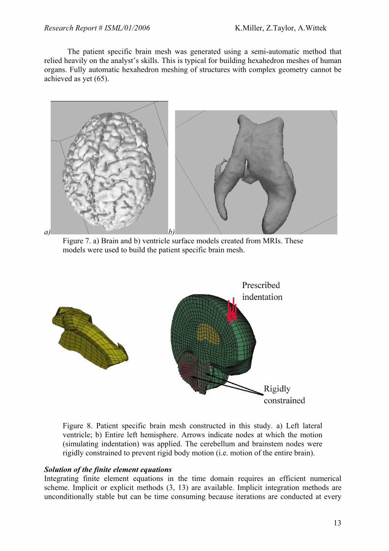
The patient specific brain mesh was generated using a semi-automatic method that relied heavily on the analyst’s skills. This is typical for building hexahedron meshes of human organs. Fully automatic hexahedron meshing of structures with complex geometry cannot be achieved as yet (65).

a) b) Figure 7. a) Brain and b) ventricle surface models created from MRIs. These models were used to build the patient specific brain mesh.

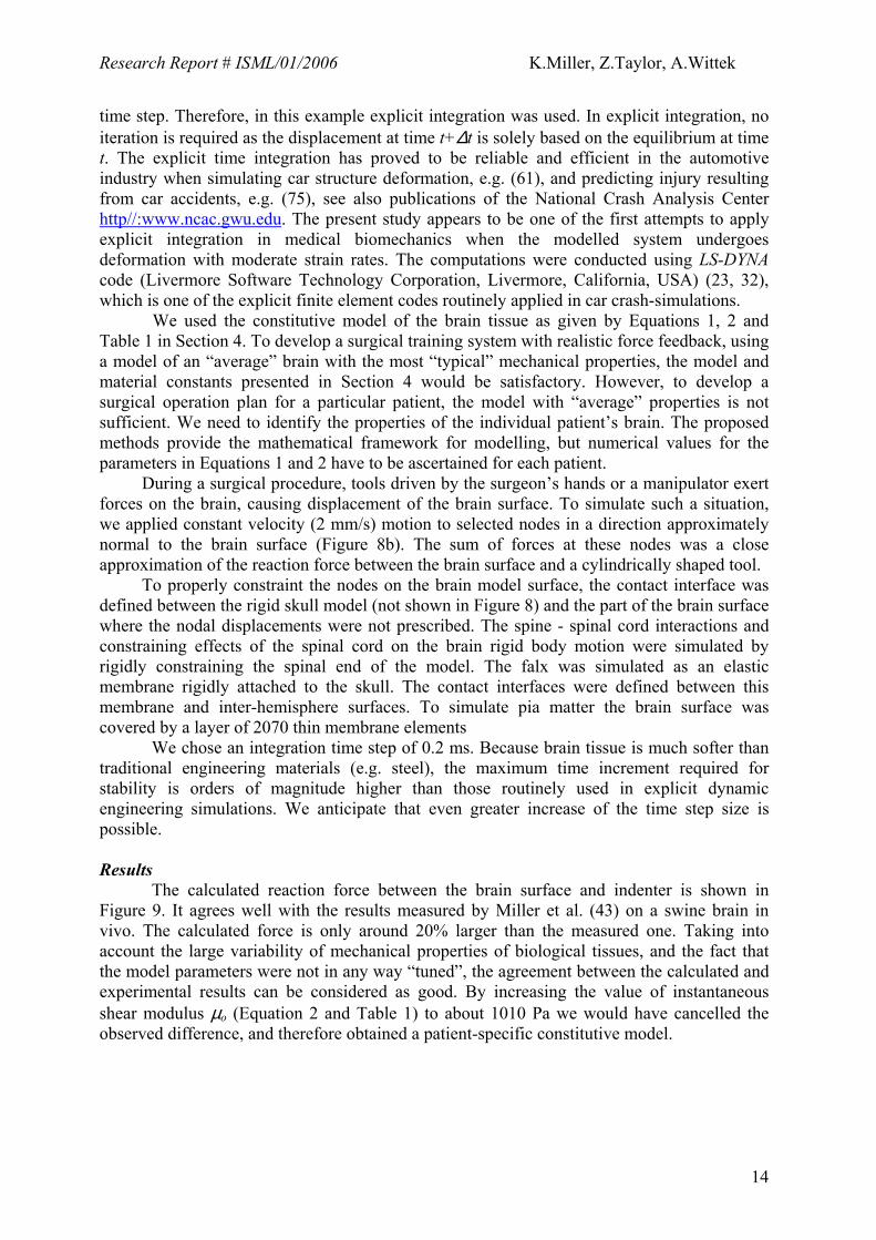
Figure 8. Patient specific brain mesh constructed in this study. a) Left lateral ventricle; b) Entire left hemisphere. Arrows indicate nodes at which the motion (simulating indentation) was applied. The cerebellum and brainstem nodes were rigidly constrained to prevent rigid body motion (i.e. motion of the entire brain).

Solution of the finite element equations Integrating finite element equations in the time domain requires an efficient numerical scheme. Implicit or explicit methods (3, 13) are available. Implicit integration methods are unconditionally stable but can be time consuming because iterations are conducted at every

13


time step. Therefore, in this example explicit integration was used. In explicit integration, no iteration is required as the displacement at time t+∆t is solely based on the equilibrium at time t. The explicit time integration has proved to be reliable and efficient in the automotive industry when simulating car structure deformation, e.g. (61), and predicting injury resulting from car accidents, e.g. (75), see also publications of the National Crash Analysis Center http//:www.ncac.gwu.edu. The present study appears to be one of the first attempts to apply explicit integration in medical biomechanics when the modelled system undergoes deformation with moderate strain rates. The computations were conducted using LS-DYNA code (Livermore Software Technology Corporation, Livermore, California, USA) (23, 32), which is one of the explicit finite element codes routinely applied in car crash-simulations.

We used the constitutive model of the brain tissue as given by Equations 1, 2 and Table 1 in Section 4. To develop a surgical training system with realistic force feedback, using a model of an “average” brain with the most “typical” mechanical properties, the model and material constants presented in Section 4 would be satisfactory. However, to develop a surgical operation plan for a particular patient, the model with “average” properties is not sufficient. We need to identify the properties of the individual patient’s brain. The proposed methods provide the mathematical framework for modelling, but numerical values for the parameters in Equations 1 and 2 have to be ascertained for each patient.

During a surgical procedure, tools driven by the surgeon’s hands or a manipulator exert forces on the brain, causing displacement of the brain surface. To simulate such a situation, we applied constant velocity (2 mm/s) motion to selected nodes in a direction approximately normal to the brain surface (Figure 8b). The sum of forces at these nodes was a close approximation of the reaction force between the brain surface and a cylindrically shaped tool.

To properly constraint the nodes on the brain model surface, the contact interface was defined between the rigid skull model (not shown in Figure 8) and the part of the brain surface where the nodal displacements were not prescribed. The spine - spinal cord interactions and constraining effects of the spinal cord on the brain rigid body motion were simulated by rigidly constraining the spinal end of the model. The falx was simulated as an elastic membrane rigidly attached to the skull. The contact interfaces were defined between this membrane and inter-hemisphere surfaces. To simulate pia matter the brain surface was covered by a layer of 2070 thin membrane elements

We chose an integration time step of 0.2 ms. Because brain tissue is much softer than traditional engineering materials (e.g. steel), the maximum time increment required for stability is orders of magnitude higher than those routinely used in explicit dynamic engineering simulations. We anticipate that even greater increase of the time step size is possible. Results

The calculated reaction force between the brain surface and indenter is shown in Figure 9. It agrees well with the results measured by Miller et al. (43) on a swine brain in vivo. The calculated force is only around 20% larger than the measured one. Taking into account the large variability of mechanical properties of biological tissues, and the fact that the model parameters were not in any way “tuned”, the agreement between the calculated and experimental results can be considered as good. By increasing the value of instantaneous shear modulus µo (Equation 2 and Table 1) to about 1010 Pa we would have cancelled the observed difference, and therefore obtained a patient-specific constitutive model.

14

http://www.ncac.gwu.edu/


Figure 9. Reaction force acting between the brain surface and the cylindrical tool versus the depth of indentation (displacement), computed using the mesh from Figure 8 and explicit time integration. The computed result agrees well with the experiment reported in (43)

The computation time was 21 minutes on a single Pentium IV 2.8 GHz processor when

simulating the indentation of 4.2 s duration. This time is clearly too long for real-time applications, and in particular for interactive simulation. We used a general-purpose engineering finite element package. It is reasonable to expect that the computation time could be significantly reduced by the application of more specialized code with reduced capabilities but improved efficiency, and by increasing the time step used in time integration of continuum mechanics equations. We estimate that using a state-of-the-art personal computer, the calculation time could be reduced to about 50 seconds (29). Improvements in computer hardware and the use of parallel processing would decrease this time even further.

Computational times of tens of seconds are acceptable for most intra-operative applications, but would still be orders of magnitude too high for applications requiring interactive simulation. Nevertheless the use of linear models, motivated by computational efficiency requirements, would not be appropriate.

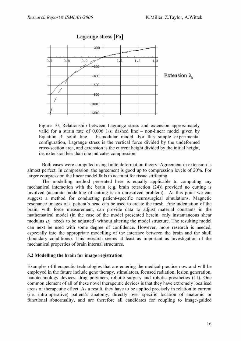
Explicit time integration algorithms avoid iterative solution of equations. A significant portion of computation time is taken by hyper-viscoelastic constitutive model evaluation (38, 42). A possible trade-off between accuracy and efficiency would be to replace the non-linear constitutive model with a bi-modular model approximately valid for a strain rate of 0.006 s-1, which is representative for neurosurgical procedures (it corresponds to the displacement of 6 mm induced with a velocity of 10 mm/s on the organ with a characteristic length of the order of 10 cm). Figure 10 presents the comparison of Lagrange stress computed using Ogden-type hyper-elastic equation:

W =2µα 2 (λ1

α + λ2α + λ3

α − 3) (5)

where µ is a shear modulus (µ=E/3 for almost incompressible materials, for a strain rate of 0.006 1/s, E=~1200 Pa) in the undeformed state and α=−4.7 is a material coefficient (38, 42), and a bi-modular model with Young’s modulus in compression Ecomp=1800 Pa and Young’s modulus in extension Eext=900 Pa.

15


Figure 10. Relationship between Lagrange stress and extension approximately valid for a strain rate of 0.006 1/s; dashed line – non-linear model given by Equation 3; solid line – bi-modular model. For this simple experimental configuration, Lagrange stress is the vertical force divided by the undeformed cross-section area, and extension is the current height divided by the initial height, i.e. extension less than one indicates compression.

Both cases were computed using finite deformation theory. Agreement in extension is

almost perfect. In compression, the agreement is good up to compression levels of 20%. For larger compression the linear model fails to account for tissue stiffening.

The modelling method presented here is equally applicable to computing any mechanical interaction with the brain (e.g. brain retraction (24)) provided no cutting is involved (accurate modelling of cutting is an unresolved problem). At this point we can suggest a method for conducting patient-specific neurosurgical simulations. Magnetic resonance images of a patient’s head can be used to create the mesh. Fine indentation of the brain, with force measurement, can provide data to adjust material constants in the mathematical model (in the case of the model presented herein, only instantaneous shear modulus µ0 needs to be adjusted) without altering the model structure. The resulting model can next be used with some degree of confidence. However, more research is needed, especially into the appropriate modelling of the interface between the brain and the skull (boundary conditions). This research seems at least as important as investigation of the mechanical properties of brain internal structures. 5.2 Modelling the brain for image registration Examples of therapeutic technologies that are entering the medical practice now and will be employed in the future include gene therapy, stimulators, focused radiation, lesion generation, nanotechnology devices, drug polymers, robotic surgery and robotic prosthetics (11). One common element of all of these novel therapeutic devices is that they have extremely localised areas of therapeutic effect. As a result, they have to be applied precisely in relation to current (i.e. intra-operative) patient’s anatomy, directly over specific location of anatomic or functional abnormality, and are therefore all candidates for coupling to image-guided

16


intervention (11). Nakaji and Spetzler (47) list the “accurate localisation of the target” as the first principle in modern neurosurgical approaches.

As only pre-operative anatomy of the patient is known precisely from scanned images (in case of the brain from pre-operative 3D MRIs), it is now recognised that one of the main problems in performing reliable surgery on soft organs is Registration. It encompasses matching images of different modality, such as standard MRI and diffusion tensor magnetic resonance imaging, functional magnetic resonance imaging or intra-operative ultrasound; defining relations between co-ordinate systems (e.g., between a co-ordinate system associated with imaging equipment and those of robotic tools in an operating room), segmentation of reference features and defining disparity or similarity functions between extracted features (30). Registration procedures involving rigid tissues are now well established. If rigidity is assumed, it is sufficient to find several points such that their mappings between two co-ordinate systems are known. Registration of soft tissues is much more difficult because it requires knowledge about local deformations. A particularly exciting application of non-rigid image registration is in intra-operative image-guided procedures, where high resolution pre-operative scans are warped onto intra-operative ones (17, 70). We are in particular interested in registering high-resolution pre-operative MRI with lower quality intra-operative imaging modalities, such as multi-planar MRI and intra-operative ultrasound. To achieve accurate matching of these modalities accurate and fast algorithms to compute tissue deformations are fundamental.

The drawback of current biomechanics model-based non-rigid registration methods is their assumed linearity (see (76) for a notable exception). Geometric non-linearities (i.e. resulting from finite deformations) are not taken into account by linear, finite element based registration methods. Certain phenomena, such as craniotomy-induced brain shift involving finite (large) displacements, cannot be reliably computed at all.

In image registration we are not interested in internal forces (stresses). Therefore, we are free to use the simplest material model available that captures the essential feature of the brain’s mechanical response: its lower stiffness in extension than in compression. The bi-modular model of Section 5.1 (Figure 10) is sufficient. Therefore, the suggested modelling approach would be to use equations of non-linear elasticity valid for finite deformations and a simple bi-modular constitutive model.

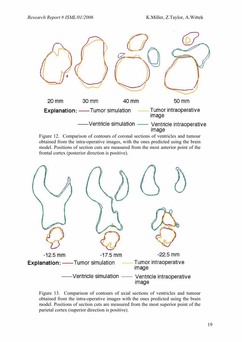
Here we present examples of computational results of brain shift, taken from (73). For this case the craniotomy-induced displacement of the tumour, as observed on intra-operative MR images, was about 7 mm. Patient-specific geometry was used. The pre- and intra-operative positions of the tumour are shown in Figure 11. The results are given in Table 2 and Figures 12 and 13.

The computed craniotomy-induced displacements of the tumour and ventricles centre of gravity (COG) agreed well with the actual ones determined from the radiographic images (Table 2). With the exception of the tumour COG displacement along the inferior-superior axis, the differences between the computed and observed displacements were below 0.65 mm. An important (and not unexpected) feature of the results summarized in Table 2 is that the displacements of the tumour and ventricle COGs differ appreciably. This feature can be explained only by the fact that the brain undergoes both local deformation and global rigid body motion (i.e. the whole brain moves), which justifies the use of non-rigid registration. It is worth noting here that linear elasticity theory is not capable of describing the deformation field that is a superposition of rigid body motion and local displacements.

Detailed comparison of cross sections of the actual tumour and ventricle surfaces acquired intra-operatively with the ones predicted by the present brain model indicates that although some local miss-registration is visible, particularly in the inferior tumour part (Figures 12 and 13), the result is remarkably good.

17


State-of-the-art image analysis methods, such as those based on optical flow (4, 25), mutual information-based similarity (66, 72), entropy-based alignment (71), and block matching (14, 57)), work perfectly well when the differences between images to be co-registered is not too large. It can be expected that the non-linear biomechanics-based model supplemented by appropriately chosen image analysis methods would provide a reliable method for brain image registration in the clinical setting.

a) b)

Figure 11. (a) Pre- and (b) intra-operative MRIs of the head. The tumour segmentation is indicated by white lines in the anterior brain part.

Table 2. Comparison of craniotomy-induced displacements of tumour and ventricles centres of gravity predicted by the present brain model with the actual ones determined from intra-operative MRIs. Coordinate axes are defined as follows: X - lateral axis; Y - vertical axis; Z - sagittal axis.

Determined from intra-

operative MRIs Predicted

∆x= 3.40 mm ∆x= 3.06 mm Ventricles ∆y= 0.25 mm ∆y= 0.29 mm ∆z= 1.73 mm ∆z= 1.65 mm ∆x= 5.36 mm ∆x= 4.74 mm Tumour ∆y=-3.52 mm ∆y=-0.40 mm ∆z= 2.64 mm ∆z= 2.77 mm

18


Figure 12. Comparison of contours of coronal sections of ventricles and tumour obtained from the intra-operative images, with the ones predicted using the brain model. Positions of section cuts are measured from the most anterior point of the frontal cortex (posterior direction is positive).

Figure 13. Comparison of contours of axial sections of ventricles and tumour obtained from the intra-operative images with the ones predicted using the brain model. Positions of section cuts are measured from the most superior point of the parietal cortex (superior direction is positive).

19


5.3. Modelling the brain for prognosis of structural diseases Brain structural diseases, such as hydrocephalus or the growth of tumours can take from hours to years to develop. Interstitial fluid flow has an important mechanical role to play in such long-lasting phenomena. Therefore, a single-phase continuum, chosen for a physical model in the previous two examples, cannot be used here. A bi-phasic continuum, consisting of a porous, deformable solid, and a penetrating fluid is more appropriate.

Since 1980 when the paper by Mow et al. (45) initiated the growth of an impressive body of knowledge related to modelling the mechanical properties of articular cartilage tissues using “bi-phasic theories”, the method has reached a high level of maturity, nevertheless should be used with caution (35). Non-linear formulations and non-linear finite element models have been developed, and solutions to real life physiological problems attempted (see (2, 64) and references cited therein). The biphasic approach has been also used for modelling the brain.

Following the work of Nagashima et al. (46) and Peña et al. (55), the biphasic nature of brain tissue may be modelled using the principles of Biot’s consolidation theory (8), which was further developed and generalized by Bowen (9). The mathematical model of the bi-phasic continuum contains equations of equilibrium, mass conservation, and fluid flow.

During the development of brain structural diseases the strain-rate is close to zero. It is therefore reasonable to adopt the limiting (hyperelastic) case of the constitutive model given by Equations 1 and 2, and Table 1 as a description of the properties of the solid phase (compare Section 5.1.2, eq.3):

)(23212ααα λλλ

αµ

++= ∞W , (6)

where: µ∞ = ~ 155 Pa is the shear modulus in the undeformed state at infinitesimally slow loading. α= -4.7.

Permeability, k = 1.59×10-7m/s, and Poisson’s ratio, ν = 0.35, are obtained from (27), and the initial void ratio for the material is taken as 0.2 (46). The fluid phase is considered to be an incompressible, inviscid fluid with the mechanical properties of water. We present an example simulation of the development of non-communicating hydrocephalus taken from our recent work (62). In a hydrocephalic brain, an obstruction may block the CSF flow and prevent its extrusion from the lateral ventricles. Consequently, ventricular fluid pressure increases and forces expansion of the ventricle walls. Because it is confined by the rigid skull (except in infantile cases) the periventricular brain parenchyma is compressed, and in acute cases, destroyed. Additionally, significant oedema is observed in the periventricular material, particularly in the regions of the frontal and occipital horns, as the increased ventricular pressure forces permeation of the CSF through the surrounding tissue. The first biomechanics-based analysis of this phenomenon was reported in (22).

Our model geometry was obtained from a horizontal cross-section presented in the anatomic atlas (51). The section was taken at 20mm above a reference defined by the anterior and posterior commissures (51). Pore pressure was fixed at zero at the skull boundary to ensure outward radial CSF flow and drainage in the sub-arachnoid space. The outer brain surface was assumed fixed to the skull and so surface nodes are constrained in all directions. Along the midline boundary, nodes are constrained in the horizontal direction (due to the presence of the left hemisphere), but are allowed to displace vertically. Loading of the ventricular wall was in the form of a distributed fluid pressure over the surface, with a magnitude of 3000Pa, in line with previous work (46, 55). Model solutions were obtained

20


using ABAQUS/Standard finite element software (1). Based on published data (46), the total development time for hydrocephalus was taken as 4 days (345600 seconds).

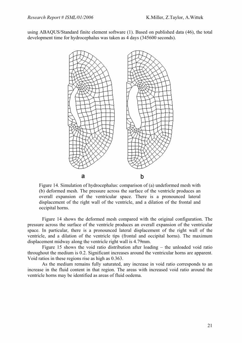
Figure 14. Simulation of hydrocephalus: comparison of (a) undeformed mesh with (b) deformed mesh. The pressure across the surface of the ventricle produces an overall expansion of the ventricular space. There is a pronounced lateral displacement of the right wall of the ventricle, and a dilation of the frontal and occipital horns.

Figure 14 shows the deformed mesh compared with the original configuration. The

pressure across the surface of the ventricle produces an overall expansion of the ventricular space. In particular, there is a pronounced lateral displacement of the right wall of the ventricle, and a dilation of the ventricle tips (frontal and occipital horns). The maximum displacement midway along the ventricle right wall is 4.79mm.

Figure 15 shows the void ratio distribution after loading – the unloaded void ratio throughout the medium is 0.2. Significant increases around the ventricular horns are apparent. Void ratios in these regions rise as high as 0.363.

As the medium remains fully saturated, any increase in void ratio corresponds to an increase in the fluid content in that region. The areas with increased void ratio around the ventricle horns may be identified as areas of fluid oedema.

21


Figure 15. Simulation of hydrocephalus: void ratio distribution. High void ratio indicates oedema. (a) entire model, (b) enlarged areas around the frontal and occipital horns with the largest void ratio

5.4 Computer simulation of the effects of the tumor growth Tumor growth can cause substantial brain deformation and change stress distribution in the tissue as well as patterns of CSF, interstitial fluid and blood flow within the brain. The bi-phasic approach would appear to be an appropriate starting mathematical modeling technique to investigate such phenomena.

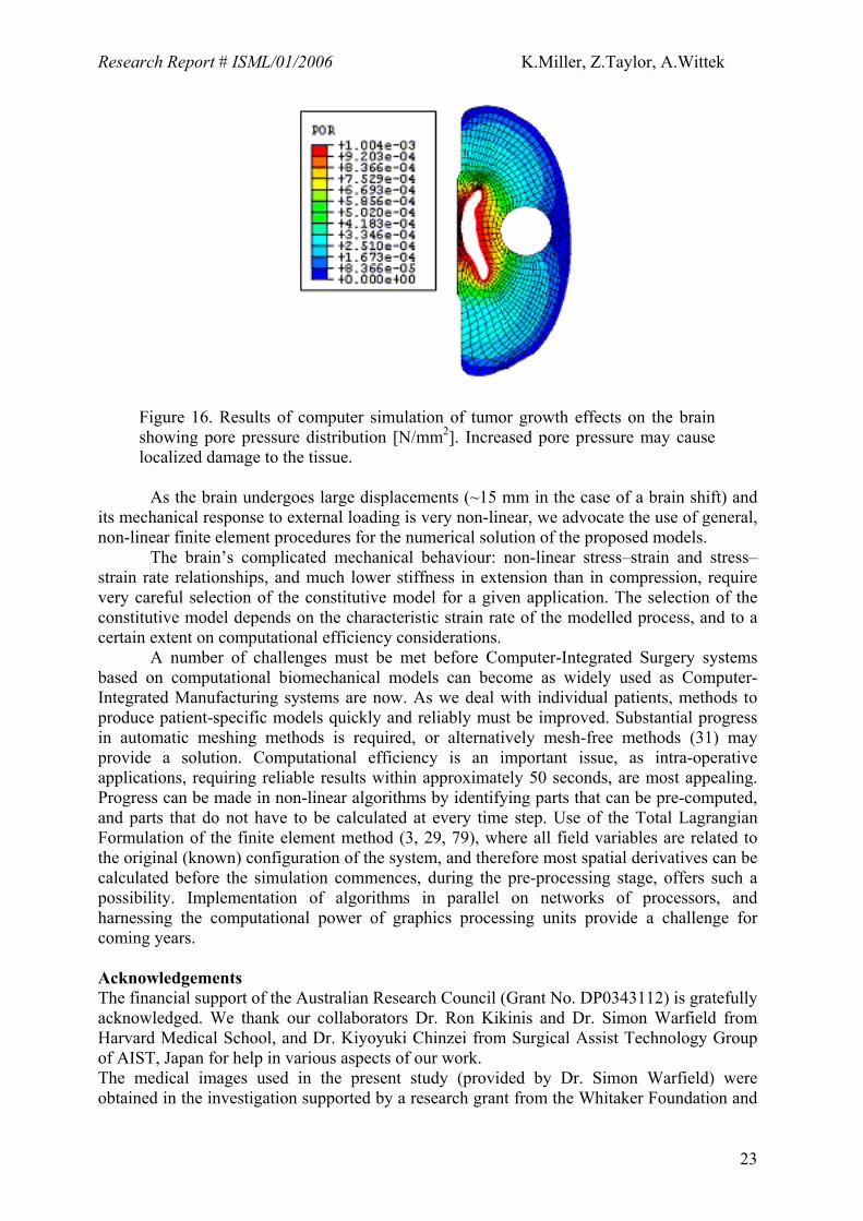
An example of the most recent results of computations conducted in our laboratory is presented here (44). The same geometry as in the simulation of hydrocephalus (Section 5.3) was used. The tumor was modeled as a rigid circle of 3 cm diameter. Figure 16 shows the calculated pore pressure distribution within the brain.

Changes of pore pressure and altered patterns of interstitial fluid flow direction and speed may have a detrimental effect on brain cell metabolism and function. The ability to predict future changes of field variables characterizing mechanical equilibrium of the brain may lead to improved prognosis and diagnosis methods. For instance, when the tumor growth rate is known, it is possible to predict the corresponding intracranial pressure.

6. Conclusions Computational mechanics has become a central enabling discipline that has led to greater understanding and advances in modern science and technology (52). It is now in a position to make a similar impact in medicine. We have discussed modelling approaches to three applications of clinical relevance: i) surgical simulation, ii) neuroimage registration, and iii) simulation of the development of structural diseases. These problems can be reasonably characterized with the use of purely mechanical terms such as displacements, internal forces, pressures, flow velocity, etc. Therefore they can be analysed using the methods of continuum mechanics.

22


Figure 16. Results of computer simulation of tumor growth effects on the brain showing pore pressure distribution [N/mm2]. Increased pore pressure may cause localized damage to the tissue.

As the brain undergoes large displacements (~15 mm in the case of a brain shift) and its mechanical response to external loading is very non-linear, we advocate the use of general, non-linear finite element procedures for the numerical solution of the proposed models. The brain’s complicated mechanical behaviour: non-linear stress–strain and stress–strain rate relationships, and much lower stiffness in extension than in compression, require very careful selection of the constitutive model for a given application. The selection of the constitutive model depends on the characteristic strain rate of the modelled process, and to a certain extent on computational efficiency considerations. A number of challenges must be met before Computer-Integrated Surgery systems based on computational biomechanical models can become as widely used as Computer-Integrated Manufacturing systems are now. As we deal with individual patients, methods to produce patient-specific models quickly and reliably must be improved. Substantial progress in automatic meshing methods is required, or alternatively mesh-free methods (31) may provide a solution. Computational efficiency is an important issue, as intra-operative applications, requiring reliable results within approximately 50 seconds, are most appealing. Progress can be made in non-linear algorithms by identifying parts that can be pre-computed, and parts that do not have to be calculated at every time step. Use of the Total Lagrangian Formulation of the finite element method (3, 29, 79), where all field variables are related to the original (known) configuration of the system, and therefore most spatial derivatives can be calculated before the simulation commences, during the pre-processing stage, offers such a possibility. Implementation of algorithms in parallel on networks of processors, and harnessing the computational power of graphics processing units provide a challenge for coming years. Acknowledgements The financial support of the Australian Research Council (Grant No. DP0343112) is gratefully acknowledged. We thank our collaborators Dr. Ron Kikinis and Dr. Simon Warfield from Harvard Medical School, and Dr. Kiyoyuki Chinzei from Surgical Assist Technology Group of AIST, Japan for help in various aspects of our work. The medical images used in the present study (provided by Dr. Simon Warfield) were obtained in the investigation supported by a research grant from the Whitaker Foundation and

23


by NIH grants R21 MH67054, R01 LM007861, P41 RR13218 and P01 CA67165. We thank Toyota Central R&D Labs. (Nagakute, Aichi, Japan) for providing the THUMS brain model.

24


Glossary of technical terms Anisotropic material – material whose properties depend on a direction in which they are

measured Bi-phasic continuum - a model that assumes the existence of two phases (e.g. a liquid and a

solid) at each point in space (in Section 5.3 deformable solid and penetrating fluid) Computational grid - a way to discretise (i.e. divide up) space so that partial differential

equations can be solved using one of the many available numerical methods Constitutive model – mathematical model describing material’s mechanical response under

loading. Usually a stress – strain, or stress – history of strain relationship Continuum – domain, within which it is assumed that physical quantities (e.g. displacement,

pressure, etc.) change from place to place in continuous way. In single-phase continuum model we assume the existence of only one phase at each point of the domain (in our case a solid). In biphasic continuum model we assume the existence of both solid and fluid at every point of the domain.

Deformation field – deformation at each point within a body Elastic material – material for which stress is proportional to strain, i.e. Hooke’s Law applies Finite deformation – deformation large enough so that it cannot be assumed to be

infinitesimal. Finite deformation elasticity – mathematical theory describing stresses and strains in materials

for arbitrarily large deformations and arbitrarily complicated material behaviour Finite element mesh – a way to discretise (i.e. divide up) space so that partial differential

equations can be solved using the finite element method Finite element method – a numerical method for solving systems of partial differential

equations. The method requires a finite element mesh. Finite element method is currently the most popular numerical method in computational mechanics

Geometric non-linearity – non-linear effects in finite deformation elasticity resulting from the change of shape and position of a body

Haptic feedback - feedback provided by a simulator by exerting forces e.g. on user’s hands Hyper-elastic material - material model, which assumes that stresses depend on strain only,

but in a complicated, non-linear way, i.e. Hooke’s Law does not apply Hyper-viscoelastic material - material model, which assumes that stresses depend on strain

and on the history of strain. This model accounts for different responses at different strain rates

Infinitesimal deformation – deformation so small that the overall position and shape of the body can be assumed constant

Incompressible material – material that does not change volume under loading Inviscid fluid – fluid with negligible viscosity, and therefore no energy dissipation within the

fluid Isotropic material – material whose properties are the same in all directions Linear elasticity – mathematical theory describing stresses and strains in materials under the

assumptions that deformations are infinitesimal and materials are elastic Permeability – parameter in bi-phasic continuum models describing how easy it is for a fluid

phase to pass through the solid phase. Unit [m/s] Poisson’s ratio – ratio of transverse strain to longitudinal strain in uniaxial extension, as

described by linear elasticity theory. For incompressible materials Poisson’s ratio is 0.5 Pressure field – pressure at each point within a body Shear modulus – parameter used in linear elasticity to relate shear stress to shear strain. Unit

[Pa = N/m2]. In simple shear, the shear modulus (µ) is a proportionality constant relating shear stress to the shear angle: shear stress = µ * tan(α), see Figure below (18).

25


ααα

Simple shear

Single-phase continuum – a model that assumes existence of only one phase at each point in

space. In Sections 4, 5.1 and 5.2 this is a deformable solid Strain – local measure of deformation. Dimensionless. In the one-dimensional case Green’s

strain is defined as the change of length divided by the initial length 0LLe ∆= ; and

Almansi’s strain is defined as the change of length divided by the current length

LLLLL ∆+=∆= 0,ε . Only for infinitesimal deformations these strain measures are

equal (18).

L0L0

L

∆LL0L0

L

∆LL0L0

L

∆L

Simple elongation

Strain rate – the speed of strain change. Unit [1/s] Stress – measure of internal forces in the material, in one-dimensional case force divided by

cross-sectional area. Unit [Pa = N/m2]. In one-dimensional extension or compression, for infinitesimal deformations, stress in many simple materials is proportional to strain and can be determined from Hooke’s Law εσ E= (where E is Young’s modulus, σ is tensile stress and ε is longitudinal strain).

Tactile feedback – feedback provided by a simulator through human sense of touch Void ration – ration of the volume of empty space (filled by fluid) to the volume of solid

phase in bi-phasic modelling approach Young’s modulus - parameter used in linear elasticity (i.e. in Hooke’s Law) to relate

longitudinal stress to longitudinal strain. εσ E= (where E is Young’s modulus, σ is tensile stress and ε is longitudinal strain). Unit [Pa = N/m2].

26


References

1. ABAQUS: ABAQUS Theory Manual Version 5.2. Hibbit, Karlsson & Sorensen, Inc.,

1998. 2. Almeida ES, Spilker RL: Mixed and Penalty Finite Element Models for the Nonlinear

Behaviour of Biphasic Soft Tissues in Finite Deformation. Comp. Meth. Biomech. Biomed. Eng. 1:25-46, 1997.

3. Bathe K-J: Finite Element Procedures. Prentice-Hall, 1996. 4. Beauchemin SS, Barron JL: The computation of optical flow. ACM Computing

Surveys 27:433-467, 1995. 5. Berry M, Bannister LH, M. SS: Nervous system, in Williams PL, Bannister LH, Berry

MM, Collins P, Dyson M, Duseek JE, Ferguson MWJ (eds): Gray`s Anatomy. The Anatomical Basis of Medicine and Surgery., Churchill Livingstone, 1990, pp 1283-1302.

6. Bilston L, Liu Z, Phan-Tiem N: Large strain behaviour of brain tissue in shear: Some experimental data and differential constitutive model. Biorheology 38:335-345, 2001.

7. Bilston LE, Zizhen L, Phan-Tien N: Linear viscoelastic properties of bovine brain tissue in shear. Biorheology 34:377-385, 1997.

8. Biot MA: General Theory of Three Dimensional Consolidation. Journal of Applied Physics 12:155-164, 1941.

9. Bowen RM: Theory of Mixtures, in Eringen AC (ed) Continuum Physics. New York, Academic Press, 1976.

10. Brands DWA, Peters GWM, Bovendeerd PHM: Design and numerical implementation of a 3-D non-linear viscoelastic constitutive model for brain tissue during impact. Journal of Biomechanics 37:127-134, 2004.

11. Bucholz R, MacNeil W, McDurmont L: The operating room of the future. Clinical Neurosurgery 51:228-237, 2004.

12. Carey GF: A Unified Approach to Three Finite Element Theories for Geometric Nonlinearity. Journal of Computer Methods in Applied Mechanics and Engineering 4:69-79, 1974.

13. Crisfield MA: Non-linear dynamics, in Non-linear Finite Element Analysis of Solids and Structures. Chichester, John Wiley & Sons, 1998, pp 447-489.

14. Dengler J, Schmidt M: The Dynamic Pyramid - A Model for Motion Analysis with Controlled Continuity. International Journal of Pattern Recognition and Artificial Intelligence 2:275-286, 1988.

15. Estes MS, J.H. M: Response of Brain Tissue of Compressive Loading. ASME Paper No. 70-BHF-13, 1970.

16. Farshad M, Barbezat M, Flüeler P, Schmidlin F, Graber P, Niederer P: Material characterization of the pig kidney in relation with the biomechanical analysis of renal trauma. Journal of Biomechanics 32:417-425, 1999.

17. Ferrant M, Nabavi A, Macq B, Jolesz FA, Kikinis R, Warfield SK: Registration of 3-D intraoperative MR images of the brain using a finite-element biomechanical model. IEEE Transactions on Medical Imaging 20:1384-1397, 2001.

18. Fung YC: A First Course In Continuum Mechanics, in. London, Prentice-Hall, 1969, p 301.

19. Fung YC: Biomechanics. Mechanical Properties of Living Tissues. New York, Springer-Verlag, 1993.

20. Fung YC: Biomechanics : circulation. New York, Springer., 1997.

27


21. Gering D, Nabavi A, Kikinis R, Hata N, Odonnell L, Grimson WEL, Jolesz F, Black P, Wells III W: An Integrated Visualization System for Surgical Planning and Guidance Using Image Fusion and an Open MR. Journal of Magnetic Resonance Imaging 13:967-975, 2001.

22. Hakim S: Biomechanics of Hydrocephalus. Acta Neurol Latinoam 17:169-174, 1971. 23. Hallquist JO: LS-DYNA Theoretical Manual. Livermore Software Technology

Corporation, 1998. 24. Hongo K, Kobayashi S, Yokoh A, Sugita K: Monitoring retraction pressure on the

brain. An experimental and clinical study. Journal of Neurosurgery 66:270-275, 1987.

25. Horn BKP, Schunk BG: Determining optical flow. Artificial Intelligence 17:185--203, 1981.

26. Iwamoto M, Watanabe I, Nakahira Y, Tamura A, Miki K: Development of a finite element model of the Total Human Model for Safety (THUMS) and application to injury reconstruction. Presented at International IRCOBI Conference on the Biomechanics of Impacts, Munich, Germany,, 2002.

27. Kaczmarek M, Subramaniam RP, Neff SR: The hydromechanics of hydrocephalus: Steady-state solutions for cylindrical geometry. Bulletin of Mathematical Biology 59:295-323, 1997.

28. Kikinis R, Shenton ME, Iosifescu DV, McCarley RW, Saiviroonporn P, Hokama HH, Robatino A, Metcalf D, Wible CG, Portas CM, Donnino R, Jolesz FA: A Digital Brain Atlas for Surgical Planning, Model Driven Segmentation and Teaching. IEEE Transactions on Visualization and Computer Graphics 2:232-241, 1996.

29. Lance D: Efficient finite element algorithm for computation of soft tissue deformations, in School of Mechanical Engineering. Perth, The University of Western Australia, 2004.

30. Lavallée S: Registration for Computer Integrated Surgery: Methodology, State of the Art, in Computer-Integrated Surgery. Cambridge, Massachusetts, MIT Press, 1995, pp 77-97.

31. Liu GR: Mesh free methods : moving beyond the finite element method. Boca Raton, Florida, CRC Press, 2003.

32. LS-DYNA: Keyword User's Manual. Version 970. Livermore, California, Livermore Software Technology Corporation, 2003.

33. Martin HC, Carey GF: Introduction to Finite Element Analysis: Theory and Application. New York, McGraw-Hill Book Co., 1973.

34. Mendis KK, Stalnaker RL, Advani SH: A constitutive relationship for large deformation finite element modeling of brain tissue. Journal of Biomechanical Engineering 117:279-285, 1995.

35. Miller K: Modelling Soft Tissue Using Biphasic Theory - A Word of Caution. Comp. Meth. Biomech. Biomed. Eng. 1:261-263, 1998.

36. Miller K: Constitutive Model of Brain Tissue Suitable for Finite Element Analysis of Surgical Procedures. Journal of Biomechanics 32:531-537, 1999.

37. Miller K: Constitutive modelling of abdominal organs. Journal of Biomechanics 33:367-373, 2000.

38. Miller K: Biomechanics of the Brain for Computer Integrated Surgery. Warsaw, Publishing House of Warsaw University of Technology, 2002.

39. Miller K, Chinzei K: Modeling of Soft Tissues. Mechanical Engineering Laboratory News 11:5-7, 1995.

40. Miller K, Chinzei K: Modeling of soft tissues deformation. Journal of Computer Aided Surgery 1:62-63, 1995.

28


41. Miller K, Chinzei K: Constitutive Modeling of Brain Tissue; Experiment and Theory. Journal of Biomechanics 30:1115-1121, 1997.

42. Miller K, Chinzei K: Mechanical properties of brain tissue in tension. Journal of Biomechanics 35:483-490, 2002.

43. Miller K, Chinzei K, Orssengo G, Bednarz P: Mechanical properties of brain tissue in-vivo: experiment and computer simulation. Journal of Biomechanics 33:1369-1376, 2000.

44. Miller K, Taylor Z, Nowinski WL: Towards computing brain deformations for diagnosis, prognosis and nerosurgical simulation. Journal of Mechanics in Medicine and Biology 5:105-121, 2005.

45. Mow VC, Kuei SC, Lai WM, Armstrong CG, ,: Biphasic Creep and Stress Relaxation of Articular Cartilage in Compression: Theory and Experiments. Trans. ASME, J. Biomech. Engng. 102:73-84., 1980.

46. Nagashima T, Tamaki N, Matsumoto S, Horwitz B, Seguchi Y: Biomechanics of Hydrocephalus: A New Theoretical Model. Neurosurgery 21:898-903, 1987.

47. Nakaji P, Speltzer RF: Innovations in Surgical Approach: The Marriage of Technique, Technology, and Judgement. Clinical Neurosurgery 51:177-185, 2004.

48. Nasseri S, Bilston LE, Phan-Thien N: Viscoelastic properties of pig kidney in shear, experimental results and modelling. Rheol Acta 41:180-192, 2002.

49. Nowinski WL: From research to clinical practice: a Cerefy brain atlas story. International Congress Series 1256:75-81, 2003.

50. Nowinski WL, Benabid AL: New directions in atlas-assisted stereotactic functional neurosurgery, in IM G (ed) Advanced Techniques in Image-Guided Brain and Spine Surgery. New York, Thieme, 2002, pp 162-174.

51. Nowinski WL, Thirunavuukarasuu, A. and Benabid, A.L.: The Cerefy Clinical Brain Atlas, in. New York, Thieme, 2003.

52. Oden JT, Belytschko T, Babuska I, Hughes TJR: Research directions in computational mechanics. Comput. Methods Appl. Mech. Engrg. 192:913-922, 2003.

53. Oden JT, Carey GF: Finite Elements: Special Problems in Solid Mechanics. Prentice-Hall, 1983.

54. Pamidi MR, Advani SH: Nonlinear Constitutive Relations for Human Brain Tissue. Trans. ASME, J. Biomech. Eng. 100:44-48, 1978.

55. Peña A, Bolton MD, Whitehouse H, Pickard JD: Effects of Brain Ventricular Shape on Periventricular Biomechanics: A Finite-element Analysis. Neurosurgery 45:107-118, 1999.

56. Prange MT, Margulies SS: Regional, directional, and age-dependent properties of the brain undergoing large deformation. ASME Journal of Biomechanical Engineering 124:244-252, 2002.

57. Rosenfeld A, Kak AC: Digital Picture Processing. New York, Academic Press, 1976. 58. Ruan JS, Khalil T, King AI: Dynamic Response of the Human Head to Impact by

Three-Dimensional Finite Element Analysis. Journal of Biomechanical Engineering 116:44-50, 1994.

59. Sahay KB, Mehrotra R, Sachdeva U, Banerji AK: Elastomechanical Characterization of Brain Tissues. J. Biomech 25:319-326, 1992.

60. Schroeder W, Martin K, Lorensem B: Visualization Toolkit: An Object-Oriented Approach to 3D Graphics. Kitware, 2002.

61. Tabiei A, Wu J: Roadmap for crashworthiness finite element simulation of roadside structures. Finite Elements in Analysis and Design 34:145-157, 2000.

62. Taylor Z, Miller K: Reassessment of brain elasticity for analysis of biomechanisms of hydrocephalus. Journal of Biomechanics 37:1263-1269, 2004.

29


63. Thibault KL, Margulies SS: Age-dependent material properties of the porcine cerebrum: effect on pediatric inertial head injury criteria. Journal of Biomechanics 31:1119-1126, 1998.

64. Van Mow C, Ateshian GA, Spilker RL: Biomechanics of diarthrodial joints: A review of twenty years of progress. Journal of Biomechanical Engineering:460-473, 1993.

65. Viceconti M, Taddei F: Automatic generation of finite element meshes from computed tomography data. Critical Reviews in Biomedical Engineering 31:27-72, 2003.

66. Viola P: Alignment by Maximization of Mutual Information, in Artificial Intelligence Laboratory, Massachusetts Institute of Technology, 1995.

67. VisibleHuman: Visible Human CD User's Guide. Version 1.0. Boulder, Colorado, Research Systems, Inc., 1995.

68. Voo L, Kumaresan S, Pintar FA, Yoganandan N, Sances J, A.: Finite-element models of the human head. Med. Biol. Eng. Comp. 34:375-381, 1996.

69. Walsh EK, Schettini A: Calculation of brain elastic parameters in vivo. Am. J. Physiol. 247:R637-R700, 1984.

70. Warfield SK, Haker, S. J., Talos, F., Kemper, C. A., Weisenfeld, N., Mewes, A. U. J., Goldberg-Zimring, D., Zou, K. H., Westin, C. F., Wells III, W. M., Tempany, C. M. C., Golby, A., Black, P. M., Jolesz, F. A., and Kikinis, R. 2005.: Capturing Intraoperative Deformations: Research Experience At Brigham and Women's Hospital. Med Image Anal. 9:145-162, 2005.

71. Warfield SK, Rexilius J, Huppi PS, Inder TE, Miller EG, Wells III WM, Zientara GP, Jolesz FA, Kikinis R: A binary entropy measure to assess nonrigid registration algorithms. Presented at 4th International Conference on Medical Image Computing and Computer Assisted Intervention MICCAI, Utrecht, The Netherlands, 2001.

72. Wells III WM, Viola P, Atsumi H, Nakajima S, Kikinis R: Multi-modal volume registration by maximization of mutual information. Medical Image Analysis 1:35-51, 1996.

73. Wittek A, Miller K, Kikinis R, Warfield S: Computation of the brain shift using a non-linear biomechanical model. Presented at 8th International Conference on Medical Image Computing and Computer Assisted Intervention, Palm Springs, California, USA, 2005.

74. Wittek A, Miller K, Laporte J, Warfield S, Kikinis R: Computing reaction forces on surgical tools for robotic neurosurgery and surgical simulation. Presented at Australasian Conference on Robotics and Automation ACRA, Canberra, Australia, 2004.

75. Wittek A, Omori K: Parametric study of effects of brain-skull boundary conditions and brain material properties on responses of simplified finite element brain model under angular acceleration in sagittal plane. JSME International Journal 46:1388-1398, 2003.

76. Xu MH, Nowinski WL: Talairach-Tournoux brain atlas registration using a metalforming principle-based finite element method. Med. Image. Anal. 5:271-279, 2001.

77. Yang KH, King AI: A limited review of finite element models developed for brain injury biomechanics research. Int. J. Vehicle Design 32:116-129, 2003.

78. Zhuang Y: Real-time Simulation of Physically Realistic Global Deformations, in Department of Computer Science, University of California at Berkley, 2000.

79. Zienkiewicz OC, Taylor RL: The Finite Element Method. London, McGRAW-HILL BOOK COMPANY, 2000.

30

Documents

MATHEMATICAL MODELS OF BRAIN DEFORMATION …isml.ecm.uwa.edu.au/ISML/images/0/0e/Isml-no-01-2006.pdf · MATHEMATICAL MODELS OF BRAIN DEFORMATION BEHAVIOUR FOR COMPUTER ... This Report