Mathematical Modeling of Action

Potential with Transmission Equations

and Hodgkin-Huxley Model

BENG 221 Problem Solving Report

Introduction

Action potential, a process during which the electrical membrane potential rapidly rises and falls

with a distinctive pattern, is almost a universal process in all organisms. Action potential exists

in neurons, muscle cells, and other types of endocrine cells. In neurons, propagation of action

potential enables the communication between neurons, leading to cognitive functions. In other

types of cells, action potential triggers cascades of intracellular processes. For instance, in

muscle cells, the propagation of action potential triggers the release of calcium and further

results in muscle contraction. Action potential is generated by voltage-gated ion channels that

respond to membrane potentials. When the incoming membrane potential is above a certain

threshold, these ion channels open. The electrochemical gradient then drives sodium and

potassium ions across membrane. Rushing in of the sodium ions is responsible for the

depolarization phase (increase in membrane potential), while outward movement of potassium

ions, which lags behind the movement of sodium ions, results in repolarization and

hyperpolarization phases. The sodium/potassium ion transporters then actively transport these

ions against their gradients to restore the original electrochemical gradients.

Propagation of action potential is such an essential process in all organisms as they are

responsible for cellular processes in multiple organs. The impairment of conduction of action

potential can lead to diseases such as multiple sclerosis or even sudden death. Here we try to use

transmission equations and Hodgkin-Huxley model to mathematically model the propagation of

action potentials as a function of time and distance. As the model depends on a wide array of

parameters, such as the input voltage, membrane capacitance, resistance, etc., with such a model

established, one can simply modify the parameters, such as these affected by a certain disease,

and examine the effects on propagation of action potential. Also, knowing the spatial and

temporal distribution of action potential of a specific can let us reversely model the parameters

and shed light on the physiological origins of certain diseases.

Set-up

An unmyelinated axon with radius a would be modeled. Current is allowed to leak back and

forth across a cylindrical membrane, every point in

the membrane, to the interstitial fluid through

capacitive and ion-transport mechanisms. Modeling

of membrane as a capacitor is reasonable because it

is thin so that the accumulation of charged particles

on one side will pull the oppositely charged particles

to the other side of the membrane. Interstitial fluid is

treated as a shunt, so it does not have resistance. The

differential equations that will be derived are also Figure 1 Excitatory postsynaptic potential and an action potential.

adapted to muscle fibers as muscle fibers are not myelinated. In our model, a voltage v is

implemented at x=0 as an initial -15 mV sawtooth impulse returning to V=0 after 3 ms (more

detailed initial and boundary conditions would be

described in the next section). A sawtooth impulse

is chosen to mimic the shape of an excitatory

postsynaptic potential (EPSP), depicted in figure 1.

In addition, as current passes through the axon, it

generates self-inductance. In summary, the axon

model can be described as the circuit diagram,

which is also the circuit for telegrapher’s equations,

in figure 2.

The differential equations that are derived from the circuit are described as following:

(1)

(2)

In which v is potential difference across membrane, i is membrane current per unit length, I is

membrane current density, ia is axon current per unit length, r is resistance per unit length of

axon material, R is specific resistance of axon, L is axon specific self-inductance, and Ca is axon

self-capacitance per unit area per unit length.

Solution

Figure 3 is the circuit diagram of Hodgkin-Huxley model. The lipid bilayer is represented as a

capacitance ( ). Voltage-gated and leak ion channels are represented by nonlinear (gn) and

linear (gL) conductances, respectively. The electrochemical gradients driving the flow of ions are

represented by batteries (E), and ion pumps and exchangers are represented by current sources

(Ip).

Figure 3 Circuit diagram for Hodgkin-Huxley model

(Reference: http://en.wikipedia.org/wiki/File:Hodgkin-Huxley.jpg)

Figure 2 Circuit diagram for axon model and telegrapher’s equations.

The time derivative of the potential across the membrane is proportional to the sum of the

currents in the circuit. This is represented as follows,

The Hodgkin-Huxley expression for I can be separated into four parallel components, the

capacitive current ( ), ion currents of potassium and sodium ( and ), and a smaller current

( ) made up of chloride and other ions.

The parameters used in the Hodgkin-Huxley equation are as follows, the specific resistances

corresponding to the component ion currents can be denoted by , , and .

From here on the

will be written as .

, , and are quantities of empirical convenience. They can also be thought of as the

probabilities of given ion in a specific location.

(3)

Where

Also, let the Vk, VNa, and Vt denote the equilibrium potential of the corresponding ions and CM

the membrane capacitance per unit area.

The full Hodgkin-Huxley excitation equation is

(4)

Now we apply

to equation (1),

,

Or

.

While using the left term of equation (2), we can get

Since

and

,

The transmission equation can be written as

(5)

Replacing the current by the value we got in equation (4), the following equation for membrane

voltage can be obtained, which combines both the processes of transmission down the axoplasm

and excitation across the membrane.

The can be replaced by without significant loss since the (

) is pretty small compared

to .

Let

,

and thus

The final partial differential equation is as follow,

Numerical Simulation

The analytical equation derived above is not one that can be easily solved. To simplify, the

equations above can be rewritten as a system of first order equations and simulated using a

finite difference method. This is accomplished by defining variables ψ and φ where ψ = and

φ = . Thus the final differential equation we obtained can be rewritten as,

Using a finite difference approach, the above equation and the hodgkin huxley parameters can

be written as,

By iterating the variables i and j, the full space and time dependent profile of voltage can be

obtained.

Figure 4: results of the finite difference method for voltage profiles over time. An action potential formed by a -15 volt

impulse is shown propagating along the axon.

The first graph shows the action potential over time across different x points which is distance

away from the input wave point. This shows how the action potential is initiated by the square

wave of -15mV and propagates along the axon (x axis) with the same peak. This makes sense

0 1 2 3 4 5 6 7 8 9 10

-120

-100

-80

-60

-40

-20

0

20

Time in milliseconds

Voltage in m

illiv

olts

Voltage profiles through time at various axon distances

because action potential is all or nothing event unlike graded potentials. The undershoot caused

by high transient potassium permeability is also apparent in the graph.

Figure 5: System response to a -5 millivolt impulse wave. The impulse is not above threshold and thus no action potential

occurs.

The second graph shows how the action potential is not achieved when an input wave of much

lower amplitude is introduced. This is important because it verifies the property of action

potential that high enough difference in membrane potential has to be introduced to trigger an

action potential. The input signal just dies out over time.

Conclusion

Our project involved using Hodgkin Huxley’s current law to derive a wave equation and

simulating the membrane potential in x and t domain using Eulers finite difference method. From

the analytical solution, the behavior of an action potential was understood as a wave equation.

0 1 2 3 4 5 6 7 8 9 10

-6

-5

-4

-3

-2

-1

0

1

2

Time in milliseconds

Voltage in m

illiv

olts

Voltage response to -5 millivolt impulse

From the numerical simulation with high enough input wave to induce an action potential, the

well-known property of an action potential was verified: An action potential is all or nothing

event that is only triggered above the certain threshold. Understanding the propagation of action

potentials is very important because it is responsible for not only communication between the

cells but also many cellular processes in multiple organs. The solutions match the current

knowledge of action potential propagation in time and space domain. And with modifications,

they could be used to model the propagation of action potential when there is a change in certain

parameter or in intensity of an input wave.

Future Work

Our model could be improved by assuming myelinated axon in which the majority of the axon is

myelinated which, in circuit, means high membrane resistance and low capacitance. This would

result in faster propagation of action potential across the axon. Using the myelination, multiple

sclerosis could be modeled and its behavior could be compared to normal myelinated axon as

well. Instead of a large change like myelination, simple modifications could be introduced to the

model when, for example, certain ion channels are damaged or ion permeability across a

membrane are altered, resulting in parameter changes in the model. The numerical

approximation method could be improved as well. In this study, Eulers finite element difference

method was used but other numerical approximation could be used such as Gram–Schmidt

process.

References

H. M. Lieberstein , On the Hodgkin-Huxley partial differential equation, Mathematical

Biosciences, 1967; 1:45-69

Stephen Waxman, “Ion channels and Neuronal Dysfunction in Multiple Sclerosis”, Arch

Neurol. 2002; 59:1377-1380

Christof Koch, “Methods in Neuronal Modeling: From synapses to networks”, 1988; ISBN 0-

262-61071-X

MATLAB SIMULATION CODE

project.m

clc; close all; clear all;

dt=0.0001; dx=1; s=dt/dx; t=0:dt:10; x=0:dx:10;

alpha_n0=0.01*(0+10)/(-1+exp((0+10)/10)); beta_n0=0.125*exp(0/80); alpha_m0=0.1*(0+25)/(-1+exp((0+25)/10)); beta_m0=4*exp(0/18); alpha_h0=0.07*exp(0/20); beta_h0=(1+exp((0+30)/10))^-1;

n=zeros(length(x),length(t)); m=zeros(length(x),length(t)); h=zeros(length(x),length(t)); v=zeros(length(x),length(t)); psi=zeros(length(x),length(t)); phi=zeros(length(x),length(t));

n(:,1)=alpha_n0/(alpha_n0+beta_n0); m(:,1)=alpha_m0/(alpha_m0+beta_m0); h(:,1)=alpha_h0/(alpha_h0+beta_h0);

%-15mV impulse for i=1:1:30000 v(1,i)=-15; end

%below threshold %for i=1:1:30000 % v(1,i)=-5; %end

for i=1:1:length(x)-1 phi(i,1)=1.5; v(i+1,1)=v(i,1)+dx*phi(i,1); end

for j=1:1:length(t)-1 %indicator for completion (in percent) j/(10/dt)*100 for i=1:1:length(x)-1 n(i,j+1)=n(i,j) + dt*N(n(i,j),v(i,j)); m(i,j+1)=m(i,j) + dt*M(m(i,j),v(i,j)); h(i,j+1)=h(i,j) + dt*H(h(i,j),v(i,j)); v(i,j+1)=v(i,j) + dt*psi(i,j);

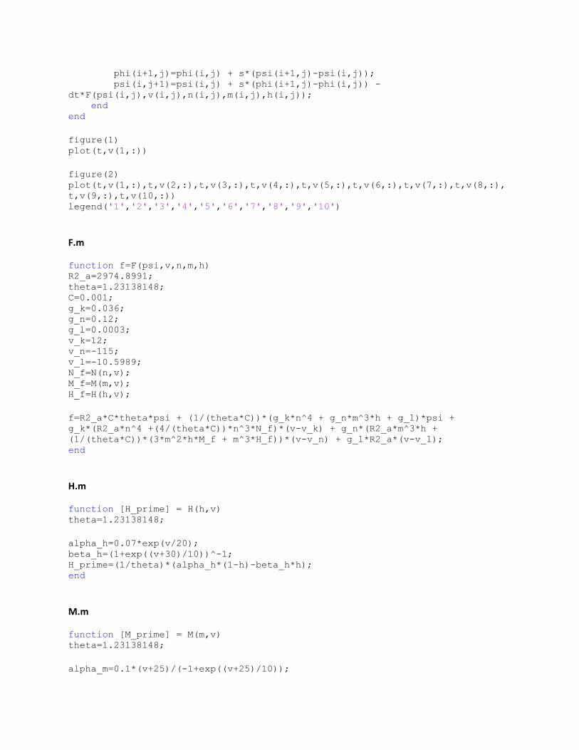
phi(i+1,j)=phi(i,j) + s*(psi(i+1,j)-psi(i,j)); psi(i,j+1)=psi(i,j) + s*(phi(i+1,j)-phi(i,j)) -

dt*F(psi(i,j),v(i,j),n(i,j),m(i,j),h(i,j)); end end

figure(1) plot(t,v(1,:))

figure(2) plot(t,v(1,:),t,v(2,:),t,v(3,:),t,v(4,:),t,v(5,:),t,v(6,:),t,v(7,:),t,v(8,:),

t,v(9,:),t,v(10,:)) legend('1','2','3','4','5','6','7','8','9','10')

F.m

function f=F(psi,v,n,m,h) R2_a=2974.8991; theta=1.23138148; C=0.001; g_k=0.036; g_n=0.12; g_l=0.0003; v_k=12; v_n=-115; v_l=-10.5989; N_f=N(n,v); M_f=M(m,v); H_f=H(h,v);

f=R2_a*C*theta*psi + (1/(theta*C))*(g_k*n^4 + g_n*m^3*h + g_l)*psi +

g_k*(R2_a*n^4 +(4/(theta*C))*n^3*N_f)*(v-v_k) + g_n*(R2_a*m^3*h +

(1/(theta*C))*(3*m^2*h*M_f + m^3*H_f))*(v-v_n) + g_l*R2_a*(v-v_l); end

H.m

function [H_prime] = H(h,v) theta=1.23138148;

alpha_h=0.07*exp(v/20); beta_h=(1+exp((v+30)/10))^-1; H_prime=(1/theta)*(alpha_h*(1-h)-beta_h*h); end

M.m

function [M_prime] = M(m,v) theta=1.23138148;

alpha_m=0.1*(v+25)/(-1+exp((v+25)/10));

beta_m=4*exp(v/18); M_prime=(1/theta)*(alpha_m*(1-m)-beta_m*m); end

N.m

function [N_prime] = N(n,v) theta=1.23138148;

alpha_n=0.01*(v+10)/(-1+exp((v+10)/10)); beta_n=0.125*exp(v/80); N_prime=(1/theta)*(alpha_n*(1-n)-beta_n*n); end