Mathematical Modeling of Continuously Variable ... · Mathematical Modeling of Continuously Variable Transmission (CVT) System Sarah Crosby* Department of Engineering Mathematics

Mathematical Modeling of Continuously Variable

Transmission (CVT) System

Sarah Crosby*

Department of Engineering Mathematics Faculty of Engineering, Alexandria University

Alexandria, Egypt

Galal Elkobrosy

Department of Engineering Mathematics

Faculty of Engineering, Alexandria University

Alexandria, Egypt

Hassan Elgamal Department of Mechanical Engineering

Faculty of Engineering, Alexandria University

Alexandria, Egypt

Abstract—A continuously variable transmission (CVT)

provides an infinite number of gear ratios between two finite

limits. This allows the engine to run at its most efficient RPM

independent of the car speed, making CVT the most efficient

transmission system. The CVT is also fuel efficient, because it

reduces the engine speed at high vehicle speed and allows the

engine to run at its optimal point.

Aiming at determining the behavior of the CVT transmission, a

complete mathematical model have been constructed for the

whole vehicle equipped with CVT, simulating the whole vehicle

dynamics. The model takes into consideration each component

of the vehicle, including: the engine dry friction disc clutch, belt

type CVT, car differential, wheels and body. In this paper, the

slip between the belt and the pulleys and the CVT traction curve

were considered. The kinematical, geometrical and momentum

equations governing the performance of the whole system were

formulated and solved. The governing differential equations

were numerically solved In order to predict the behavior of the

different mechanical parts of the system. The results of the

simulation shows that the system becomes steady after a short

period of time. The analysis of the system’s dynamical response

demonstrates that the simulation model established represents

the system efficiently.

Keywords— Automatic Transmission; Continuously variable

transmission; Mathematical Modeling; Transmission; ; V-belt

CVT

I. INTRODUCTION

Over the last decades, a growing attention has been focused on

the environmental question. Governments are continuously

forced to set standards and to adopt actions in order to reduce

the polluting emissions and the green-house gasses. In order to

fulfil these requirements, car manufacturers have been

obligated to dramatically reduce vehicles' gas emissions. The

continuously variable transmission (CVT) represents one of

the most promising solution, which is able to provide an

infinite number of gear ratios between two finite limits. The

CVT optimizes the engine working conditions, gets the

highest efficiency, and therefore, improves fuel saving and

reduces greenhouse gases emissions

With the lack of oil and the call for reducing the

environmental pollutants, the number of cars equipped with

CVT has significantly increased. Up to now, more than one

billon cars have been equipped with continuously variable

transmission all over the world. Especially the metal belt type

continuously variable transmission is applied widely. CVT

has wide change range of speed ratio and it can adjust the ratio

continuously and automatically according to the situation of

running to maintain the engine to work in economy mode or

power mode all the time. For this reason, CVT equipped cars

are more economical than cars equipped with planetary gear

automatic transmissions. The key advantages of a CVT that

interest vehicle manufacturers and customers can be

summarized as: higher engine efficiency, higher fuel

economy, smooth acceleration without shift shocks and

Infinite gear ratios with a small number of parts.

A continuously variable transmission (CVT) is an automatic

transmission that can change seamlessly through an infinite

number of effective gear ratios between maximum and

minimum values by changing the diameters of input shaft and

output shaft directly, instead of going through several gears to

perform gear ratio change. This contrasts with other

mechanical transmissions that offer a fixed number of gear

ratios. The most common type of CVT used is the pulley

based CVT. The variable-diameter pulleys are main

component of the pulley-based CVT. Each pulley is made of

two 20-degree cones facing each other. A belt rides in the

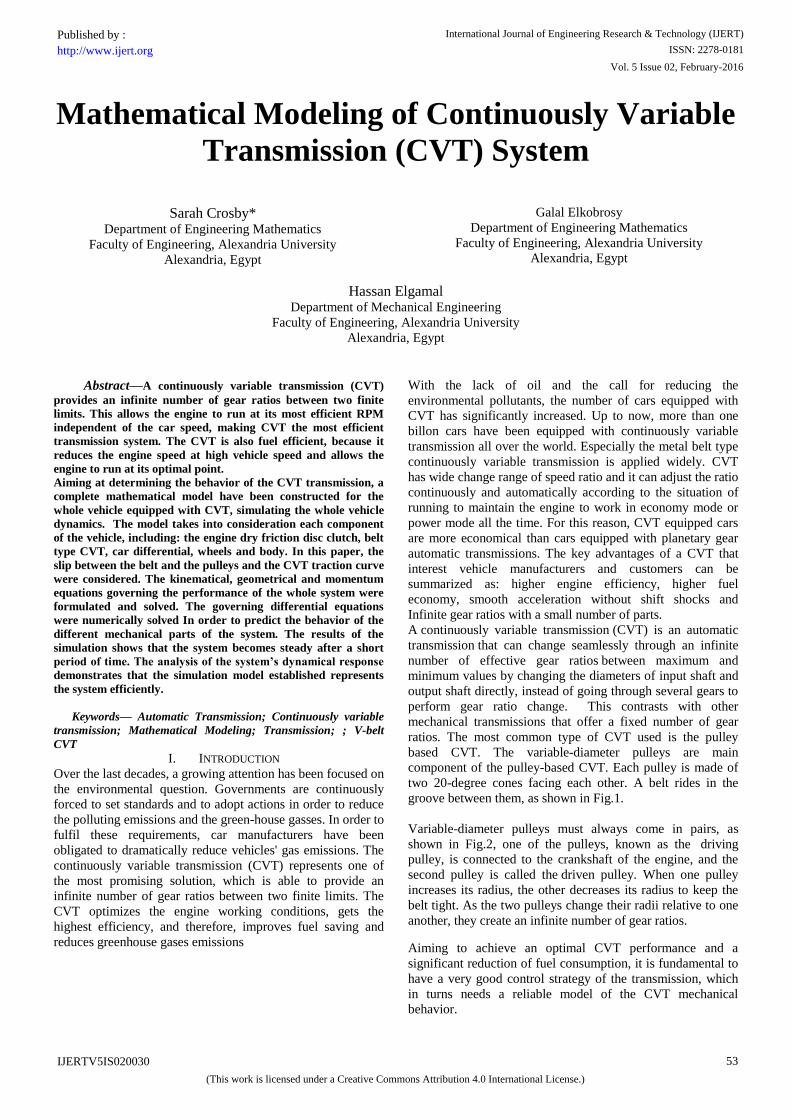
groove between them, as shown in Fig.1.

Variable-diameter pulleys must always come in pairs, as

shown in Fig.2, one of the pulleys, known as the driving

pulley, is connected to the crankshaft of the engine, and the

second pulley is called the driven pulley. When one pulley

increases its radius, the other decreases its radius to keep the

belt tight. As the two pulleys change their radii relative to one

another, they create an infinite number of gear ratios.

Aiming to achieve an optimal CVT performance and a

significant reduction of fuel consumption, it is fundamental to

have a very good control strategy of the transmission, which

in turns needs a reliable model of the CVT mechanical

behavior.

International Journal of Engineering Research & Technology (IJERT)

ISSN: 2278-0181http://www.ijert.org

IJERTV5IS020030

(This work is licensed under a Creative Commons Attribution 4.0 International License.)

Published by :

Vol. 5 Issue 02, February-2016

53

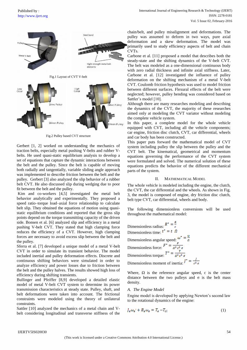
Fig.1 Layout of CVT V-belt

Fig.2 Pulley based CVT structure

Gerbert [1, 2] worked on understanding the mechanics of

traction belts, especially metal pushing V-belts and rubber V-

belts. He used quasi-static equilibrium analysis to develop a

set of equations that capture the dynamic interactions between

the belt and the pulley. Since the belt is capable of moving

both radially and tangentially, variable sliding angle approach

was implemented to describe friction between the belt and the

pulley. Gerbert [3] also analyzed the slip behavior of a rubber

belt CVT. He also discussed slip during wedging due to poor

fit between the belt and the pulley.

Kim and co-workers [4,5] investigated the metal belt

behavior analytically and experimentally. They proposed a

speed ratio–torque load–axial force relationship to calculate

belt slip. They obtained the equations of motion using quasi-

static equilibrium conditions and reported that the gross slip

points depend on the torque transmitting capacity of the driven

side. Bonsen et al. [6] analyzed slip and efficiency in a metal

pushing V-belt CVT. They stated that high clamping force

reduces the efficiency of a CVT. However, high clamping

forces are necessary to avoid excess slip between the belt and

the pulley.

Sferra et al. [7] developed a unique model of a metal V-belt

CVT in order to simulate its transient behavior. The model

included inertial and pulley deformation effects. Discrete and

continuous shifting behaviors were simulated in order to

analyze efficiency and power losses due to friction between

the belt and the pulley halves. The results showed high loss of

efficiency during shifting transients.

Bullinger and Pfeiffer [8,9] developed a detailed elastic

model of metal V-belt CVT system to determine its power

transmission characteristics at steady state. Pulley, shaft, and

belt deformations were taken into account. The frictional

constraints were modeled using the theory of unilateral

constraints.

Sattler [10] analyzed the mechanics of a metal chain and V-

belt considering longitudinal and transverse stiffness of the

chain/belt, and pulley misalignment and deformations. The

pulley was assumed to deform in two ways, pure axial

deformation and a skew deformation. The model was

primarily used to study efficiency aspects of belt and chain

CVTs.

Carbone et al. [11] proposed a model that describes both the

steady-state and the shifting dynamics of the V-belt CVT.

The belt was modeled as a one-dimensional continuous body

with zero radial thickness and infinite axial stiffness. Later,

Carbone et al. [12] investigated the influence of pulley

deformation on the shifting mechanism of a metal V-belt

CVT. Coulomb friction hypothesis was used to model friction

between different surfaces. Flexural effects of the belt were

neglected; however, pulley bending was considered based on

Sattler’s model [10].

Although there are many researches modeling and describing

the dynamics of the CVT, the majority of these researches

aimed only at modeling the CVT variator without modeling

the complete vehicle system.

In this paper, a complete model for the whole vehicle

equipped with CVT, including all the vehicle components;

car engine, friction disc clutch, CVT, car differential, wheels

and car body has been constructed.

This paper puts forward the mathematical model of CVT

system including pulley the slip between the pulley and the

CVT belt. The kinematical, geometrical and momentum

equations governing the performance of the CVT system

were formulated and solved. The numerical solution of these

equations predicts the behavior of the different mechanical

parts of the system.

II. MATHEMATICAL MODEL

The whole vehicle is modeled including the engine, the clutch,

the CVT, the car differential and the wheels. As shown in Fig.

3, the model is composed of engine, dry friction disc clutch,

belt type CVT, car differential, wheels and body.

The following dimensionless conversions will be used

throughout the mathematical model:

Dimensionless radius:

Dimensionless time:

Dimensionless angular speed:

Dimensionless force:

Dimensionless torque:

Dimensionless moment of inertia:

Where, Ω is the reference angular speed, c is the center

distance between the two pulleys and σ is the belt mass

density.

A. The Engine Model

Engine model is developed by applying Newton’s second law

to the rotational dynamics of the engine:

(1)



IJERTV5IS020030


Published by :


54

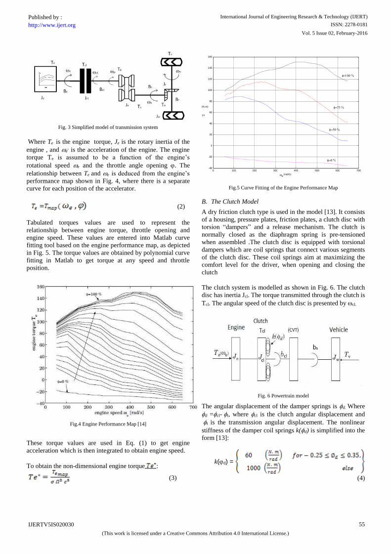
Fig. 3 Simplified model of transmission system

Where Te is the engine torque, Je is the rotary inertia of the

engine , and e. is the acceleration of the engine. The engine

torque Te is assumed to be a function of the engine’s

rotational speed e and the throttle angle opening . The

relationship between Te and e is deduced from the engine’s

performance map shown in Fig. 4, where there is a separate

curve for each position of the accelerator.

(2)

Tabulated torques values are used to represent the

relationship between engine torque, throttle opening and

engine speed. These values are entered into Matlab curve

fitting tool based on the engine performance map, as depicted

in Fig. 5. The torque values are obtained by polynomial curve

fitting in Matlab to get torque at any speed and throttle

position.

Fig.4 Engine Performance Map [14]

These torque values are used in Eq. (1) to get engine

acceleration which is then integrated to obtain engine speed.

To obtain the non-dimensional engine torque :

(3)

Fig.5 Curve Fitting of the Engine Performance Map

B. The Clutch Model

A dry friction clutch type is used in the model [13]. It consists

of a housing, pressure plates, friction plates, a clutch disc with

torsion “dampers” and a release mechanism. The clutch is

normally closed as the diaphragm spring is pre-tensioned

when assembled .The clutch disc is equipped with torsional

dampers which are coil springs that connect various segments

of the clutch disc. These coil springs aim at maximizing the

comfort level for the driver, when opening and closing the

clutch

The clutch system is modelled as shown in Fig. 6. The clutch

disc has inertia Jcl. The torque transmitted through the clutch is

Tcl. The angular speed of the clutch disc is presented by cl.

Fig. 6 Powertrain model

The angular displacement of the damper springs is d. Where

d =cl-t, where cl is the clutch angular displacement and

t is the transmission angular displacement. The nonlinear

stiffness of the damper coil springs k(d) is simplified into the

form [13]:

k(d) =

(4)

0 100 200 300 400 500 600 700 -40

-20

0

20

40

60

80

100

120

140

160

e (rad/s)

T e

(N.m)



IJERTV5IS020030


Published by :


55

The differential equations governing the clutch dynamics can

be expressed as:

(5)

(6)

The torque through the clutch while slipping is given by:

(7) In which is the friction coefficient of the clutch surface

material, is the active radius of the clutch plates and the

normal actuation force on the clutch plate is given by .

The dimensionless clutch torque can be obtained by:

(8) Where:

(9)

C. CVT and drive shafts:

1) CVT Model Assumptions

The model that will be presented is derived by making the

following assumptions and simplifications:

a) The metal belt is considered as a one-dimensional

continuous body, with locally rigid motion. This

means there is no longitudinal and transversal

deformation, i.e. the belt is considered to be an

inextensible strip with zero radial thickness and

infinite axial stiffness.

b) The bending stiffness of the belt is neglected.

c) The Coulomb friction coefficient μ, acting between

the segments and the pulleys, has a constant

value.

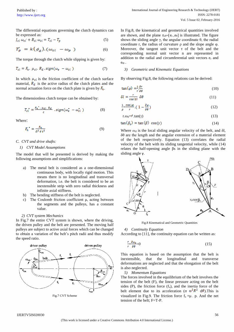
2) CVT system Mechanics

In Fig.7 the entire CVT system is shown, where the driving,

the driven pulley and the belt are presented. The moving half

pulleys are subject to active axial forces which can be changed

to obtain a variation of the belt’s pitch radii and thus modify

the speed ratio.

Fig.7 CVT Scheme

In Fig.8, the kinematical and geometrical quantities involved

are shown, and the plane rereis illustrated. The figure

shows the sliding angle γ, the angular coordinate θ, the radial

coordinate r, the radius of curvature ρ and the slope angle φ.

Moreover, the tangent unit vector τ of the belt and the

corresponding normal unit vector n are represented in

addition to the radial and circumferential unit vectors er and

eΘ .

3) Geometric and Kinematic Equations

By observing Fig.8, the following relations can be derived:

. (10)

(11)

= . (12)

r.d= .tan() (13)

(14)

Where ωd is the local sliding angular velocity of the belt, and δl,

δθ are the length and the angular extension of a material element

of the belt respectively. Equation (13) correlates the radial

velocity of the belt with its sliding tangential velocity, while (14)

relates the half-opening angle βs in the sliding plane with the

sliding angle γ.

Fig.8 Kinematical and Geometric Quantities

4) Continuity Equation

According to [11], the continuity equation can be written as:

+ =0 (15)

This equation is based on the assumption that the belt is

inextensible, that the longitudinal and transverse

deformations are neglected and that the elongation of the belt

is also neglected.

5) Momentum Equations

The forces involved in the equilibrium of the belt involves the

tension of the belt (F), the linear pressure acting on the belt

sides (P), the friction force (fa), and the inertia force of the

belt element due to its acceleration (σ d ).This is

visualized in Fig.9. The friction force fa =p. And the net

tension of the belt; F=T-P.



IJERTV5IS020030


Published by :


56

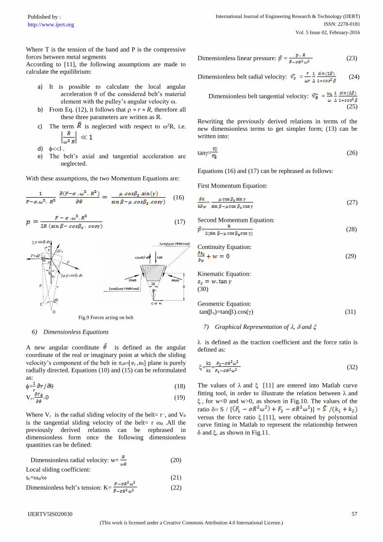
Where T is the tension of the band and P is the compressive

forces between metal segments

According to [11], the following assumptions are made to

calculate the equilibrium:

a) It is possible to calculate the local angular

acceleration θ of the considered belt’s material

element with the pulley’s angular velocity ω.

b) From Eq. (12), it follows that ≈ r ≈ R, therefore all

these three parameters are written as R.

c) The term is neglected with respect to ω2R, i.e.

d) .

e) The belt’s axial and tangential acceleration are

neglected.

With these assumptions, the two Momentum Equations are:

(16)

(17)

Fig.9 Forces acting on belt

6) Dimensionless Equations

A new angular coordinate is defined as the angular

coordinate of the real or imaginary point at which the sliding

velocity’s component of the belt in rere plane is purely

radially directed. Equations (10) and (15) can be reformulated

as:

= (18)

Vr+ =0 (19)

Where Vr is the radial sliding velocity of the belt= r ., and V

is the tangential sliding velocity of the belt= r d .All the

previously derived relations can be rephrased in

dimensionless form once the following dimensionless

quantities can be defined:

Dimensionless radial velocity: w= (20)

Local sliding coefficient:

sc=d/(21

Dimensionless belt’s tension: K= (22)

Dimensionless linear pressure: = (23)

Dimensionless belt radial velocity: = (24)

Dimensionless belt tangential velocity: =

(25)

Rewriting the previously derived relations in terms of the

new dimensionless terms to get simpler form; (13) can be

written into:

tan= (26)

Equations (16) and (17) can be rephrased as follows:

First Momentum Equation:

= (27)

Second Momentum Equation:

= (28)

Continuity Equation:

(29)

Kinematic Equation:

(30)

Geometric Equation:

tan(s)=tan().cos() (31)

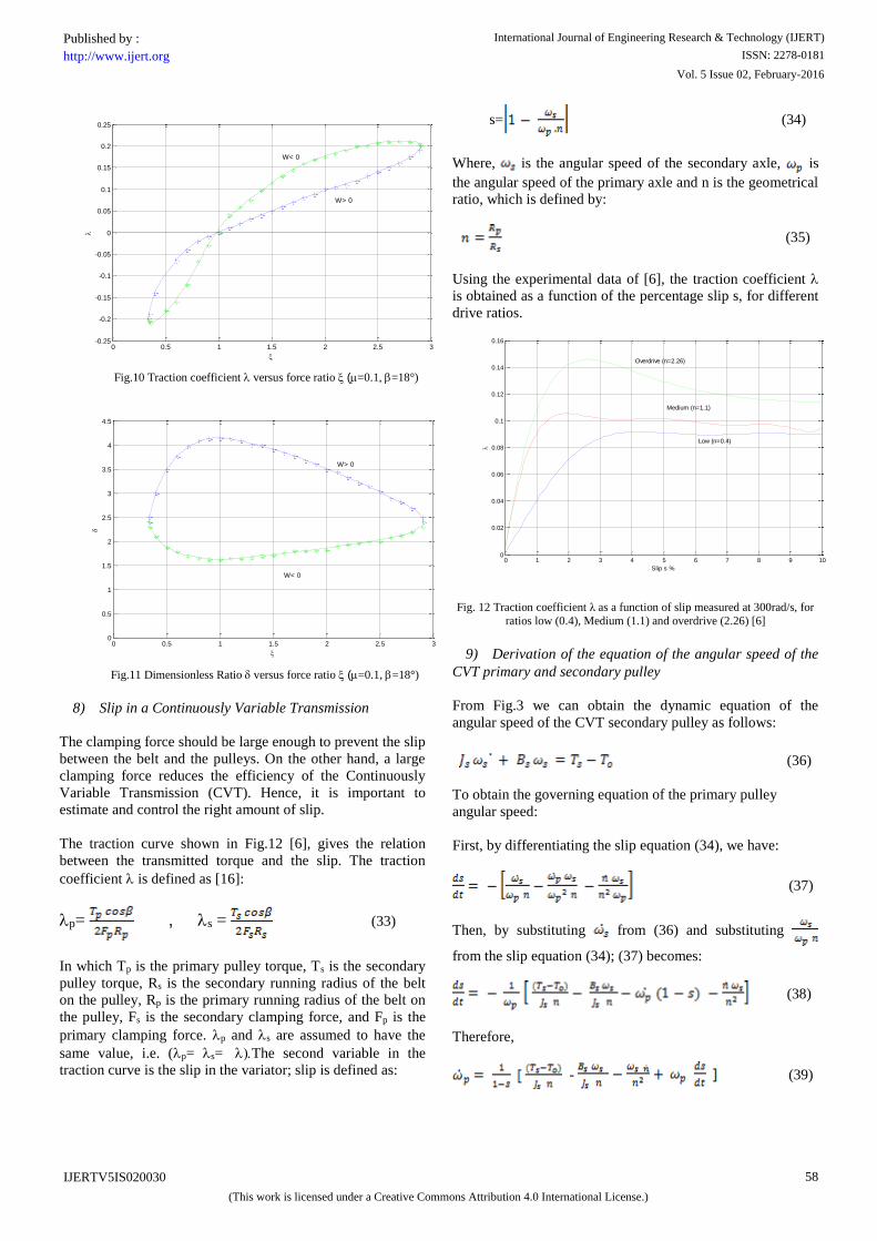
7) Graphical Representation of and

is defined as the traction coefficient and the force ratio is

defined as:

= = (32)

The values of and [11] are entered into Matlab curve

fitting tool, in order to illustrate the relation between and

for w<0 and w>0, as shown in Fig.10. The values of the

ratio S / [ )] =

versus the force ratio [11], were obtained by polynomial

curve fitting in Matlab to represent the relationship between

and as shown in Fig.11.



IJERTV5IS020030


Published by :


57

0 0.5 1 1.5 2 2.5 3-0.25

-0.2

-0.15

-0.1

-0.05

0

0.05

0.1

0.15

0.2

0.25

W< 0

W> 0

Fig.10 Traction coefficient versus force ratio (=0.1, =18°)

0 0.5 1 1.5 2 2.5 30

0.5

1

1.5

2

2.5

3

3.5

4

4.5

W< 0

W> 0

Fig.11 Dimensionless Ratio versus force ratio (=0.1, =18°)

8) Slip in a Continuously Variable Transmission

The clamping force should be large enough to prevent the slip

between the belt and the pulleys. On the other hand, a large

clamping force reduces the efficiency of the Continuously

Variable Transmission (CVT). Hence, it is important to

estimate and control the right amount of slip.

The traction curve shown in Fig.12 [6], gives the relation

between the transmitted torque and the slip. The traction

coefficient is defined as [16]:

p= , s = (33)

In which Tp is the primary pulley torque, Ts is the secondary

pulley torque, Rs is the secondary running radius of the belt

on the pulley, Rp is the primary running radius of the belt on

the pulley, Fs is the secondary clamping force, and Fp is the

primary clamping force. p and s are assumed to have the

same value, i.e. (p= s= The second variable in the

traction curve is the slip in the variator; slip is defined as:

s= (34)

Where, is the angular speed of the secondary axle, is

the angular speed of the primary axle and n is the geometrical

ratio, which is defined by:

(35)

Using the experimental data of [6], the traction coefficient

is obtained as a function of the percentage slip s, for different

drive ratios.

0 1 2 3 4 5 6 7 8 9 100

0.02

0.04

0.06

0.08

0.1

0.12

0.14

0.16

Slip s %

Low (n=0.4)

Medium (n=1.1)

Overdrive (n=2.26)

Fig. 12 Traction coefficient λ as a function of slip measured at 300rad/s, for

ratios low (0.4), Medium (1.1) and overdrive (2.26) [6]

9) Derivation of the equation of the angular speed of the

CVT primary and secondary pulley

From Fig.3 we can obtain the dynamic equation of the

angular speed of the CVT secondary pulley as follows:

(36)

To obtain the governing equation of the primary pulley

angular speed:

First, by differentiating the slip equation (34), we have:

(37)

Then, by substituting from (36) and substituting

from the slip equation (34); (37) becomes:

(38)

Therefore,

- (39)



IJERTV5IS020030


Published by :


58

And in dimensionless form:

- (

(40)

In order to obtain :

By differentiation the traction coefficient equation (33) w.r.t

time we get:

(41)

From the clutch model equation, (6) and from (41), we have:

(42)

But, . Let

Therefore,

(43)

From the traction coefficient equation (33):

(44)

Substituting from (44) into (42) we get,

(45)

Substituting from (45) into (34) we get,

= (46)

In dimensionless form:

(47)

10) Calculation of dimensionless primary and secondary

radius

The values of the radii of the primary and secondary pulleys

are functions of the ratio between the belt length and the

center distance of the two pulleys. The length of the belt can

be calculated from the following relation:

L = + sin-1 +

(48)

Dividing the previous equation by the center distance, we

have:

(49)

The belt length in dimensionless form is given by:

(50)

Assuming the value of and getting the roots of the non-

linear equation of y using Matlab, the values of and

can be calculated.

11) Evaluation of the values of and

The non-dimensional ratiois obtained by using the

versus slip relation, in Fig.12, knowing the value of speed

ratio ‘n’ and the allowed value of slip percentage. And is

obtained from the relation between and in Fig.10,

according to the sign of dimensionless radial velocity .

Where:

(51)

The ratio is obtained from the relation between and in

Fig.11, according to the sign of the dimensionless radial

velocity .

12) Evaluation of the primary and secondary torques

Since,

Hence,

(52)

Since,

Hence,

(53)

From (33) we have,

(54)

Substituting from (54) into (52):

(55) Substituting From (53) into (55)



IJERTV5IS020030


Published by :


59

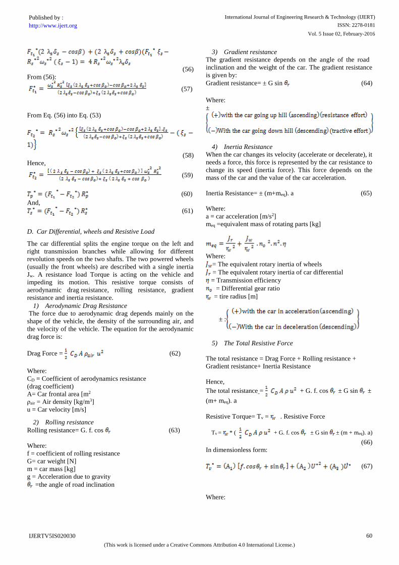
(56)

From (56):

(57)

From Eq. (56) into Eq. (53)

(58)

Hence,

(59)

(60)

And, (61)

D. Car Differential, wheels and Resistive Load

The car differential splits the engine torque on the left and

right transmission branches while allowing for different

revolution speeds on the two shafts. The two powered wheels

(usually the front wheels) are described with a single inertia

Jw. A resistance load Torque is acting on the vehicle and

impeding its motion. This resistive torque consists of

aerodynamic drag resistance, rolling resistance, gradient

resistance and inertia resistance.

1) Aerodynamic Drag Resistance

The force due to aerodynamic drag depends mainly on the

shape of the vehicle, the density of the surrounding air, and

the velocity of the vehicle. The equation for the aerodynamic

drag force is:

Drag Force = (62)

Where:

CD = Coefficient of aerodynamics resistance

(drag coefficient)

A= Car frontal area [m2

ρair = Air density [kg/m3]

u = Car velocity [m/s]

2) Rolling resistance

Rolling resistance= G. f. cos (63)

Where:

f = coefficient of rolling resistance

G= car weight [N]

m = car mass [kg]

g = Acceleration due to gravity

=the angle of road inclination

3) Gradient resistance

The gradient resistance depends on the angle of the road

inclination and the weight of the car. The gradient resistance

is given by:

Gradient resistance= ± G sin (64)

Where:

±

4) Inertia Resistance

When the car changes its velocity (accelerate or decelerate), it

needs a force, this force is represented by the car resistance to

change its speed (inertia force). This force depends on the

mass of the car and the value of the car acceleration.

Inertia Resistance= ± (m+meq). a (65)

Where:

a = car acceleration [m/s2]

meq =equivalent mass of rotating parts [kg]

Where:

= The equivalent rotary inertia of wheels

= The equivalent rotary inertia of car differential

= Transmission efficiency

= Differential gear ratio

= tire radius [m]

± :

5) The Total Resistive Force

The total resistance = Drag Force + Rolling resistance +

Gradient resistance+ Inertia Resistance

Hence,

The total resistance = + G. f. cos ± G sin ±

(m+ meq). a

Resistive Torque= Tv = . Resistive Force

Tv = * ( + G. f. cos ± G sin ± (m + meq). a)

(66)

In dimensionless form:

(67)

Where:



IJERTV5IS020030


Published by :


60

A1= , A2= , A3= +

From Fig.3 we can obtain the dynamic equation of the

vehicle angular speed as follows:

(68)

E. Evaluation of the load torque on CVT

can be obtained from the following relation :

III. NUMERICAL SOLUTION, RESULTS AND DISCUSSION

From (1), (5), (36), (40) and (68), the governing ordinary

differential equations of the vehicle mathematical model can

be written as follows:

-

(

In which, Je, is the rotary inertia of engine; Jcl, is the rotary

inertia of clutch; Js is the rotary inertia of the secondary

pulley of CVT; Jr is the rotary inertia of the car differential;

and Jw is the rotary inertia of the wheels. And Be, Bcl, Bs and

Br represent the equivalent damping coefficient of each axis

respectively

A. The initial Conditions

At the beginning of the motion when t*=0, the initial

conditions are:

B. Numerical Solution

The ordinary differential equations were numerically solved

using ode23 MATLAB solver. The ode23 solver uses second

and third order Runge-Kutta-Fehlberg integration with

variable step size. The angular speeds of each component of

the model were integrated with time. The results are plotted

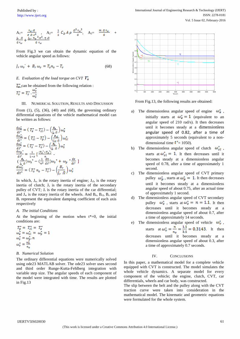
in Fig.13

0 500 1000 1500 2000 2500 3000 3500 4000 4500 50000.2

0.3

0.4

0.5

0.6

0.7

0.8

0.9

1

1.1

1.2

ecl

p

s

v

Time (t*)

Dim

ensio

nle

ss A

ngula

r S

peeds

From Fig.13, the following results are obtained:

a) The dimensionless angular speed of engine ,

initially starts at (equivalent to an

angular speed of 210 rad/s). It then decreases

until it becomes steady at a dimensionless angular speed of 0.82, after a time of approximately 5 seconds (equivalent to a non-

dimensional time = 1050).

b) The dimensionless angular speed of clutch ,

starts at . It then decreases until it

becomes steady at a dimensionless angular

speed of 0.78, after a time of approximately 1

second.

c) The dimensionless angular speed of CVT primary

pulley , starts at . It then decreases

until it becomes steady at a dimensionless

angular speed of about 0.75, after an actual time

of approximately 1 second.

d) The dimensionless angular speed of CVT secondary

pulley , starts at . It then

decreases until it becomes steady at a

dimensionless angular speed of about 0.7, after

a time of approximately 14 seconds.

e) The dimensionless angular speed of vehicle ,

starts at . It then

decreases until it becomes steady at a

dimensionless angular speed of about 0.3, after

a time of approximately 0.7 seconds.

IV. CONCLUSIONS

In this paper, a mathematical model for a complete vehicle

equipped with CVT is constructed. The model simulates the

whole vehicle dynamics. A separate model for every

component of the vehicle; the engine, clutch, CVT, car

differentials, wheels and car body, was constructed.

The slip between the belt and the pulley along with the CVT

traction curve were taken into consideration in the

mathematical model. The kinematic and geometric equations

were formulated for the whole system.



IJERTV5IS020030


Published by :


61

The differential equations for the angular velocities for every

component in the system were formulated. These equations

were numerically solved in order to predict the behavior of

the system. Plotting the angular speeds with time, the

numerically simulated results show that the system becomes

steady after a short period of time. The graphical

representation of the system’s dynamical response

demonstrates that the simulation model established represent

the system efficiently.

REFERENCES

[1] G. Gerbert, Force and slip behavior in V-belt drives, Acta Polytechnica Scandinavica, Mechanical Engineering Series, No. 67, Lund Technical University, Lund, Sweden, 1972.

[2] G. Gerbert, Metal V-belt mechanics, in: ASME Design Automation Conference, Advances in Design Automation, ASME Paper No. 84-DET-227, Boston, MA, 1984, 9p.

[3] G. Gerbert, Belt slip – a unified approach, ASME Journal of Mechanical Design 118 (3) (1996) 432–438.

[4] H. Kim, J. Lee, Analysis of belt behavior and slip characteristics for a metal V-belt CVT, Mechanism and Machine Theory 29 (6) (1994) 865–876.

[5] H. Lee, H. Kim, Analysis of primary and secondary thrust for a metal CVT, Part 1: new formula for speed ratio–torque–thrust relationship considering band tension and block compression, in: Transmission and Driveline Symposium, SAE Paper No. 2000-01-0841, SAE special publication (SP-1522), 2000, pp. 117–125.

[6] B. Bonsen, T.W.G.L. Klaassen, K.G.O. van de Meerakker, M. Steinbuch, P.A. Veenhui36zen, Analysis of slip in a continuously variable transmission, in: Proceedings of IMECE’03, 2003 ASME International Mechanical Engineering Congress, Paper No.

IMECE2003-41360, Washington, DC, USA, vol. 72, No. 2, November 15–21, 2003, pp. 995–1000.

[7] D. Sferra, E. Pennestri, P.P. Valentini, F. Baldascini, Dynamic simulation of a metal-belt CVT under transient conditions, in: Proceedings of the ASME 2002 Design Engineering Technical Conference, Paper No. DETC02/MECH-34228, Montreal, Canada, vol. 5A, September 29–October 2, 2002, pp. 261– 268.

[8] M. Bullinger, F. Pfeiffer, Elastic modelling of bodies and contacts in continuous variable transmissions, Multibody System Dynamics 13 (2) (2005) 175–194.

[9] M. Bullinger, F. Pfeiffer, An elastic model of a metal V-belt CVT, Proceedings in Applied Mathematics and Mechanics (PAMM) 2 (2003) 112 113.

[10] H. Sattler, Efficiency of metal chain and V-belt CVT, in: Proceedings of the International Congress on Continuously Variable Power Transmission CVT’99, Eindhoven, The Netherlands, September 16–17, 1999, pp. 99–104.

[11] G. Carbone, L. Mangialardi, G. Mantriota, The influence of pulley deformations on the shifting mechanism of metal belt CVT, ASME Journal of Mechanical Design 127 (1) (2005) 103–113.

[12] G. Carbone, L. Mangialardi, B. Bonsen, C. Tursi, P.A. Veenhuizen, CVT dynamics: theory and experiments, Mechanism and Machine Theory 42 (4) (2007) 409–428.

[13] A.F.A. Serrarens, M. Dassen, and M. Steinbuch. Simulation and control of an automotive dry clutch. In Proceedings of the American Control Conference, pages 4078–4083, Boston, USA, 2004.

[14] A. F. A. Serrarens. Coordinated Control of The Zero Inertia Powertrain. PhD thesis, Technische Universiteit Eindhoven, 2001.

[15] G. Gerbert, F. Sorge, Full sliding adhesive-like contact of V-belts, ASME Journal of Mechanical Design 124 (4) (2002) 706–712.

[16] B. Bonsen, R.J. Pulles, S.W.H. Simons, M. Steinbuch, P.A. Veenhuizen, Implementation of a slip controlled CVT in a production vehicle, in: Proceedings of the 2005 IEEE Conference on Control Applications, Toronto, Canada, August 28–31, 2005, pp. 1212–1217.



IJERTV5IS020030


Published by :


62

Documents

Mathematical Modeling of Continuously Variable ... · Mathematical Modeling of Continuously Variable Transmission (CVT) System Sarah Crosby* Department of Engineering Mathematics