Embed Size (px)
Citation preview

MATH 2XX3 - Advanced Calculus II
Prof. S. Alama 1
♦Class notes recorded, adapted, and illustrated
by Sang Woo Park♦
Revised March 5, 2019
1 c©2017, 2018 by S. Alama and S.W. Park. All Rights Reserved. Not to be distributed without authors’permission.

Contents
Preface iii
Bibliography iv
1 Space, vectors, and sets 11.1 Vector norms . . . . . . . . . . . . . . . . . . . . . . . . . . . . . . . . . . . 11.2 Subsets of Rn . . . . . . . . . . . . . . . . . . . . . . . . . . . . . . . . . . . 51.3 Practice problems . . . . . . . . . . . . . . . . . . . . . . . . . . . . . . . . . 8
2 Functions of several variables 92.1 Limits and continuity . . . . . . . . . . . . . . . . . . . . . . . . . . . . . . . 92.2 Differentiability . . . . . . . . . . . . . . . . . . . . . . . . . . . . . . . . . . 132.3 Chain rule . . . . . . . . . . . . . . . . . . . . . . . . . . . . . . . . . . . . . 192.4 Practice problems . . . . . . . . . . . . . . . . . . . . . . . . . . . . . . . . . 22
3 Paths, directional derivative, and gradient 233.1 Paths and curves . . . . . . . . . . . . . . . . . . . . . . . . . . . . . . . . . 233.2 Directional derivatives and gradient . . . . . . . . . . . . . . . . . . . . . . . 303.3 Gradients and level sets . . . . . . . . . . . . . . . . . . . . . . . . . . . . . 323.4 Lagrange multipliers . . . . . . . . . . . . . . . . . . . . . . . . . . . . . . . 333.5 Practice Problems . . . . . . . . . . . . . . . . . . . . . . . . . . . . . . . . . 38
4 The geometry of space curves 394.1 The Frenet frame and curvature . . . . . . . . . . . . . . . . . . . . . . . . . 394.2 Dynamics . . . . . . . . . . . . . . . . . . . . . . . . . . . . . . . . . . . . . 444.3 Practice problems . . . . . . . . . . . . . . . . . . . . . . . . . . . . . . . . . 46
5 Implicit functions 475.1 The Implicit Function Theorem I . . . . . . . . . . . . . . . . . . . . . . . . 475.2 The Implicit Function Theorem II . . . . . . . . . . . . . . . . . . . . . . . . 515.3 Inverse Function Theorem . . . . . . . . . . . . . . . . . . . . . . . . . . . . 535.4 Practice problems . . . . . . . . . . . . . . . . . . . . . . . . . . . . . . . . . 56
6 Taylor’s Theorem and critical points 596.1 Taylor’s Theorem in one dimension . . . . . . . . . . . . . . . . . . . . . . . 596.2 Taylor’s Theorem in higher dimensions . . . . . . . . . . . . . . . . . . . . . 606.3 Local minima/maxima . . . . . . . . . . . . . . . . . . . . . . . . . . . . . . 636.4 Practice problems . . . . . . . . . . . . . . . . . . . . . . . . . . . . . . . . . 71
i

7 Calculus of Variations 737.1 One-dimensional problems . . . . . . . . . . . . . . . . . . . . . . . . . . . . 737.2 Problems in higher dimensions . . . . . . . . . . . . . . . . . . . . . . . . . . 807.3 Practice problems . . . . . . . . . . . . . . . . . . . . . . . . . . . . . . . . . 82
8 Fourier Series 858.1 Fourier’s Crazy, Brilliant Idea . . . . . . . . . . . . . . . . . . . . . . . . . . 858.2 Orthogonality . . . . . . . . . . . . . . . . . . . . . . . . . . . . . . . . . . . 868.3 Fourier Series . . . . . . . . . . . . . . . . . . . . . . . . . . . . . . . . . . . 888.4 Pointwise and Uniform Convergence . . . . . . . . . . . . . . . . . . . . . . . 928.5 Orthogonal families . . . . . . . . . . . . . . . . . . . . . . . . . . . . . . . . 102
8.5.1 The Gram-Schmidt process . . . . . . . . . . . . . . . . . . . . . . . 1028.5.2 Eigenvalue problems . . . . . . . . . . . . . . . . . . . . . . . . . . . 103
8.6 Convergence in Norm . . . . . . . . . . . . . . . . . . . . . . . . . . . . . . . 1068.7 Application: The vibrating string . . . . . . . . . . . . . . . . . . . . . . . . 1098.8 Practice problems . . . . . . . . . . . . . . . . . . . . . . . . . . . . . . . . . 111

Preface
These notes are intended as a kind of organic textbook for a class in advanced calculus, forstudents who have already studied three terms of calculus (from a standard textbook suchas Stewart [Stew],) and one or two terms of linear algebra.
Typically, these two subjects (calculus and linear algebra) have been introduced as sep-arate areas of study, and aside from some small intersection the true intertwined natureof multivariable and vector calculus with linear algebra has been hidden. For example, inStewart the derivative of multivariable functions is only discussed in special cases, intro-ducing only the partial derivatives and certain physically important combinations (curl anddivergence,) but avoiding the discussion of the derivative as a linear transformation (ie, amatrix.) As a consequence, the notion of differentiability is not properly presented. Inaddition, the chain rule is presented as an ad hoc collection of separate formulas dealingwith specific cases of composite functions, together with some visual tricks to make themeasier to calculate. There are many other instances where mysterious looking calculationtechniques are introduced in order to avoid a more powerful and general formulation viamatrices and linear maps. This is because standard calculus books cannot assume thatstudents have linear algebra as a prerequisite or corequisite course.
A second issue which we address here is the level and mathematical content of themultivariable calculus introduced in the first three terms. In a mixed audience with notonly mathematics students but also physicists, engineers, biologists, economists, etc, theemphasis in the calculus class is on formulas, calculation, and problem solving directedto the applications of calculus, and less stress is put on the actual mathematics. This canlead to a shock when students encounter higher level mathematics, such as real and complexanalysis or topology, where calculational proficiency becomes secondary to an understandingof when and why mathematical facts are true. In this course we will pay careful attentionto precise definitions, and the need to verify that they are satisfied in specific examples.Facts will be presented as Theorems, and students will need to understand the hypthesesand the conclusions, how they apply (or not) to specific cases, and what their consequencesare. Some computation will be needed to do examples, but we will make a step up inmathematical rigor and the emphasis will be on understanding the definitions and theorems.
The topics presented here begin with the foundations of multivariable calculus: a discus-sion of the structure of Euclidean space Rn, followed by limits and continuity, the derivative,and important properties of the derivative. This covers Chapters 1–3. The succeeding chap-ters are more or less independent of each other and may be covered in any order (and somemay be deemed optional.) Chapter 4 concerns the differential geometry of curves in R3,with the Frenet frame and curvature. The Implicit and Inverse Function Theorems are thesubject of Chapter 5. Chapter 6 introduces the second-order Taylor’s Theorem in order tounderstand the role of the second derivative matrix in classifying critical points. Chapter 7
iii

CHAPTER 0. PREFACE iv
is an introduction to the Calculus of Variations, which puts together many aspects of theprevious material in the study of extremal problems in spaces of functions. And finally, inChapter 8 we introduce Fourier Series and orthogonal decompositions, a field which is tooimportant to mathematics and its applications to be relegated to more specialized classesin partial differential equations. (An inexpensive paperback Dover book by Tolstov [Tol] isalso used for this segment of the course.)
Why write these notes when there are so many calculus textbooks on the market? It’strue that there are some excellent books dealing with advanced calculus in a way which in-troduces correct mathematical definitions and statements of theorems, without introducingthe difficulties of rigorously proving all of the (fairly complex) theorems of vector calculus;the book by Marsden & Tromba [MT] is one. However, these books are intended as areplacement for Stewart, and spend many pages on developing the calculation techniqueswhich students have already learned in the 3-term calculus sequence. And the linear alge-bra background presumend by [MT] is actually much less than what students learn in the2-semester linear algebra sequence 1B03–2R03. More advanced books, such as Marsden &Hoffman [MH], are really analysis books and the level is too high for a second-year course.And so we have a need for an intermediate level text.
Fortunately, a student, Sang Woo Park, made a LaTeX transcription of his class notesfor Math 2XX3 in the Winter 2017 term, which he generously offered to his fellow studentson his personal web page as the document evolved. Sang Woo then added some graphics toillustrate various concepts, and this text was born!
Finally, I will be keeping a corrected copy and a list of corrections on the course webpage. If you find an error, or some place where the text is unclear, (and it doesn’t alreadyappear on the list of corrections,) please send me email at [email protected] so I canmake the correction.
Prof. S. Alama, McMaster University, October 2017. Revised March 5, 2019

Bibliography
[AR] H. Anton and C. Rorres. Elementary Linear Algebra: Applications Version, 11thEdition:. Wiley Global Education, 2013.
[MH] J. Marsden and M. Hoffman. Elementary Classical Analysis. W. H. Freeman, 1993.
[MT] J. E. Marsden and A. Tromba. Vector calculus. Macmillan, 2003.
[Stew] J. Stewart. Calculus: Early Transcendentals. Cengage Learning, 2015.
[Tol] G. Tolstov. Fourier Series. Dover Books on Mathematics. Dover Publications, 2012.
v

BIBLIOGRAPHY vi

Chapter 1
Space, vectors, and sets
Over the last three terms you’ve studied (at least) two flavors of mathematics: calculus
and linear algebra. They have been taught separately, and probably feel very different to
you. Linear Algebra is about vectors and matrices, and how you use them to solve linear
algebraic equations. Calculus is about functions, continuity, and rates of change. The main
goal of this course is to bring these two subjects together. Indeed, to understand calculus
in more than one dimension it is essential to use concepts from linear algebra. And the
constructions from linear algebra (which may have seemed strange and arbitrary to you
when you learned them) are then motivated by their use in understanding calculus in the
plane and in space.
We begin by a brief discussion of space,
Rn = {(x1, x2, . . . , xn) : x1, x2, . . . , xn ∈ R},
where it all happens.
1.1 Vector norms
To connect linear algebra to calculus we need to talk about lengths and distance. This is
done via a norm.
Definition 1.1. Euclidean norm of ~x = (x1, x2, . . . , xn) is given as
‖~x‖ =√~x · ~x =
√√√√ n∑j=1
x2j
Using the norm we can then define the distance between any two points ~p and ~q in Rn,
dist(~p, ~q) = ‖~p− ~q‖.
Notice that this also suggests that the “norm” of a “’vector” x ∈ R1 = R (and R is a vector
space!) should be defined by
‖x‖ =√x2 = |x|,
1
CHAPTER 1. SPACE, VECTORS, AND SETS 2
so in one dimension the distance is defined via the absolute value,
dist(p, q) = |p− q|, ∀p, q ∈ R.
In dimension n ≥ 2 the Euclidean norm is intimately related to the dot product of
vectors,
~x · ~y =n∑i=1
xi yi,
which gives us the useful concept of orthogonality: ~x ⊥ ~y when ~x · ~y = 0. More generally,
the dot product enables us to calculate angles between vectors:
~x · ~y = ‖~x‖ ‖~y‖ cos θ,
where θ is the angle between ~x and ~y, drawn in the plane determined by the two vectors.
Since | cos θ| ≤ 1 for any angle, we also have the famous
Theorem 1.2 (Cauchy-Schwartz Inequality).
|~x · ~y| ≤ ‖~x‖ ‖~y‖
The Euclidean norm has certain properties, which are intuitively clear if we think about
it as measuring the length of a vector:
Theorem 1.3 (Properties of a norm).
1. ‖~x‖ ≥ 0 and ‖~x‖ = 0 iff ~x = ~0 = (0, 0, . . . , 0).
2. For all scalars a ∈ R, ‖a~x‖ = |a| · ‖~x‖.
3. (Triangle inequality) ‖~x+ ~y‖ ≤ ‖~x‖+ ‖~y‖.
Proof. (i) If ~x = ~0, then by the formula ‖~0‖ =√
0 = 0. On the other hand, if ‖~x‖ = 0, then
0 = ‖~x‖2 =n∑i=1
x2i .
This is a sum of squares, so each term in the sum is non-negative, and thus each must equal
zero. This proves (i).
For (ii), this is just factoring (and being careful that√a2 = |a|!!)
‖a~x‖ =
√√√√a2n∑i=1
x2i = |a|
√√√√ n∑i=1
x2i = |a|‖~x‖.

CHAPTER 1. SPACE, VECTORS, AND SETS 3
For (iii), we look at the square of the norm, which is easier than that norm itself:
‖~x+ ~y‖2 = (~x+ ~y) · (~x+ ~y) = ~x · ~x+ ~y · ~y + 2~x · ~y = ‖~x‖2 + ‖~y‖2 + 2~x · ~y≤ ‖~x‖2 + ‖~y‖2 + 2‖~x‖ ‖~y‖= (‖~x‖+ ‖~y‖)2.
Since each term is non-negative, we can take the square root of each side to obtain the
triangle inequality (iii).
Remark. It is easy to verify that in R1 = R, ‖x‖ = |x| satisfies all the above properites of
the norm. The first two conditions are immediate. To verify the triangle inequality, we use
the fact that |x|2 = x2, so
|x+ y|2 = (x+ y)2 = x2 + y2 + 2xy ≤ x2 + y2 + 2|x| |y| = |x|2 + |y|2 + 2|x| |y| = (|x|+ |y|)2.
As above, each term is non-negative, so we take the square root to obtain the triangle
inequality for the absolute value,
|x+ y| ≤ |x|+ |y| (1.1)
We separate out the properties in this way to point out that there may be many other
ways of measuring the length of a vector in Rn (which give different numerical values) which
would be equally valid as norms.
Example 1.4 (A non-Euclidean norm - The Taxi Cab Norm). Consider the vector ~p =
(p1, p2) ∈ R2. The euclidean norm gives the length of the diagonal line joining ~0 to ~p. On
the other hand,
‖~p‖1 = |p1|+ |p2|gives us the length traveled in a rectangular grid system, like the number of blocks traveled
in a car in a city of streets meeting at right angles. We can define a taxi cab norm in any
dimension: for ~p = (p1, p2, . . . , pn) ∈ Rn, ‖~p‖1 =∑n
j=1 |pj|.As with the Euclidean norm, we may define the distance between two points ~p, ~q ∈ Rn
as the taxi cab norm length of the vector joining them, dist1(~p, ~q) = ‖~p− ~q‖1. In the plane,
this is the number of city blocks (east-west plus north-south) you need to drive to get from
one point to the other. Unless the two points lie on the same street (and can be joined by a
segment parallel to one of the axes), the distance will be larger than the Euclidean distance,
which is the distance “as the bird flies” from one point to the other along the (diagonal)
straight line path.
The Taxi Cab norm is a valid norm because it satisfies all properties of a norm above.
(You will show this as an exercise!) So it also gives us a valid alternative way to measure
distance in Rn, dist(~p, ~q) = ‖~p − ~q‖. This way of measuring distance gives Rn a different
geometry, as we will see below. (However, this norm is not compatible with the dot product,
as you will also see from the exercise below.)

CHAPTER 1. SPACE, VECTORS, AND SETS 4
Definition 1.5. The Neighborhood of radius r > 0 about a point ~p is the set
Dr(~p) ={~x ∈ Rn
∣∣‖~x− ~p‖ < r}
We may also call this the disk of radius r > 0 in R2, or the ball of radius r > 0 in R3.
Remark. Different books use different notations for a neighborhood, and so depending on
which of the calculus books you read, the neighborhood around ~a of radius r may be written
using any of the following notations:
Dr(~a) = Br(~a) = B(~a, r)
Definition 1.6. The sphere of radius r > 0 about ~p is defined as
Sr(~p) ={~x ∈ Rn
∣∣‖~x− ~p‖ = r}
The shape of the neighborhood and sphere depends strongly on which norm you choose.
First, let’s start with the familiar Euclidean norm. Then, the sphere is given by
‖~x− ~p‖ = r
⇐⇒
√√√√ n∑j=1
(xj − pj)2 = r,
which is equivalent ton∑j=1
(xj − pj)2 = r2.
When n = 3, we have
(x1 − p1)2 + (x2 − p2)2 + (x3 − p3)2 = r2,
the usual sphere in R3 with center ~p = (p1, p2, p3)
When n = 2, we have
(x1 − p1)2 + (x2 − p2)2 = r2,
the usual circle in Rn with center ~p = (p1, p2).
If we replace Euclidean norm by the Taxi Cab norm (for simplicity, take ~p = ~0), we have
Staxir (~0) =
{~x ∈ Rn
∣∣‖~x−~0‖1 = r}
In other words, we have
~x ∈ Staxir (~0) ⇐⇒
n∑j=1
|xj| = r
CHAPTER 1. SPACE, VECTORS, AND SETS 5
1
2
−1
−2
1 2−1−2
x
y
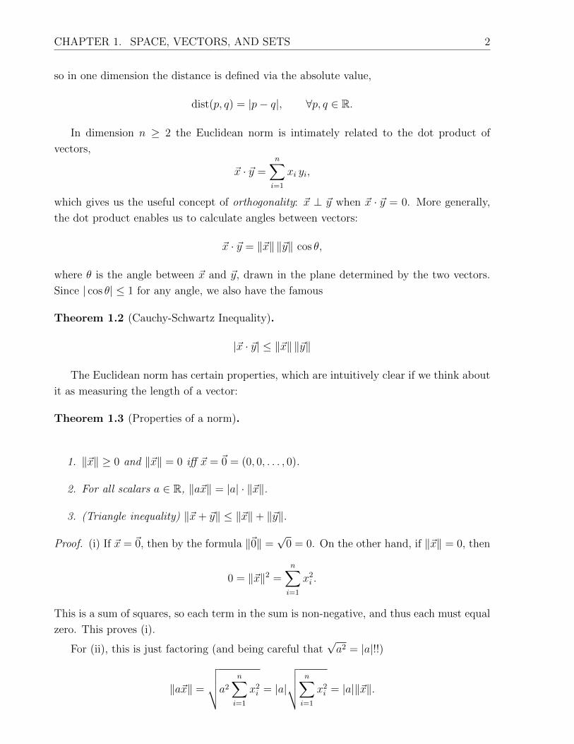
Figure 1.1. Neighborhood around (0, 0) of radius 1 using the Taxi Cab norm.
In R2, we have ~x = (x1, x2). Then, r = |x1| + |x2|, which is a diamond. (See figure 1.1)1.
Notice that in the first quadrant, x1, x2 ≥ 0, we have x1 + x2 = r, which is the line segment
with slope −1 connecting (r, 0) to (0, r). In the second quadrant, |x1| = −x1 and so the
equation of the taxi cab circle is −x1 +x2 = r, the segment with slope +1 joining (−r, 0) to
(0, r). The two other segments (in the third and fourth quadrants) forming the taxi-sphere
may be derived in a similar manner.
1.2 Subsets of Rn
Let’s introduce some properties of subsets in Rn. A ⊂ Rn means A is a collection of points
~x, drawn from Rn.
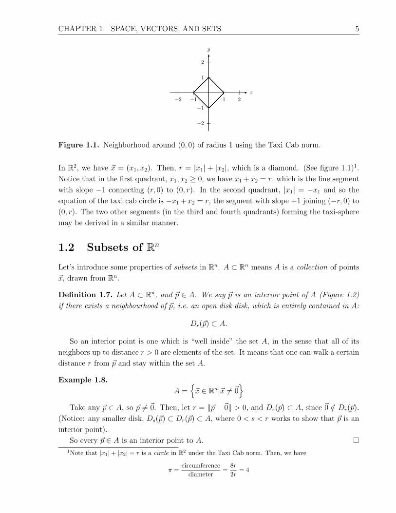
Definition 1.7. Let A ⊂ Rn, and ~p ∈ A. We say ~p is an interior point of A (Figure 1.2)
if there exists a neighbourhood of ~p, i.e. an open disk disk, which is entirely contained in A:
Dr(~p) ⊂ A.
So an interior point is one which is “well inside” the set A, in the sense that all of its
neighbors up to distance r > 0 are elements of the set. It means that one can walk a certain
distance r from ~p and stay within the set A.
Example 1.8.
A ={~x ∈ Rn|~x 6= ~0
}Take any ~p ∈ A, so ~p 6= ~0. Then, let r = ‖~p− ~0‖ > 0, and Dr(~p) ⊂ A, since ~0 /∈ Dr(~p).
(Notice: any smaller disk, Ds(~p) ⊂ Dr(~p) ⊂ A, where 0 < s < r works to show that ~p is an
interior point).
So every ~p ∈ A is an interior point to A.
1Note that |x1|+ |x2| = r is a circle in R2 under the Taxi Cab norm. Then, we have
π =circumference
diameter=
8r
2r= 4

CHAPTER 1. SPACE, VECTORS, AND SETS 6
x
y
r
r
Figure 1.2. The point on the left is an interior point; the point on the right is aboundary point.
Definition 1.9. If every ~p ∈ A is an interior point, we call A an open set.
Example 1.10. A ={~x ∈ Rn|~x 6= ~0
}is an open set.
Proposition 1.11. A = DR(~0) is an open set.
Proof. If ~p = ~0, Dr(~0) ⊆ A = DR(~0) provided r ≤ R. So ~p = ~0 is interior to A. Consider
any other ~p ∈ A. It’s evident that Dr(~p) ⊂ A = DR(~0) provided that 0 ≤ r ≤ R − ‖~p‖.Therefore, A = DR(~0) is an open set.
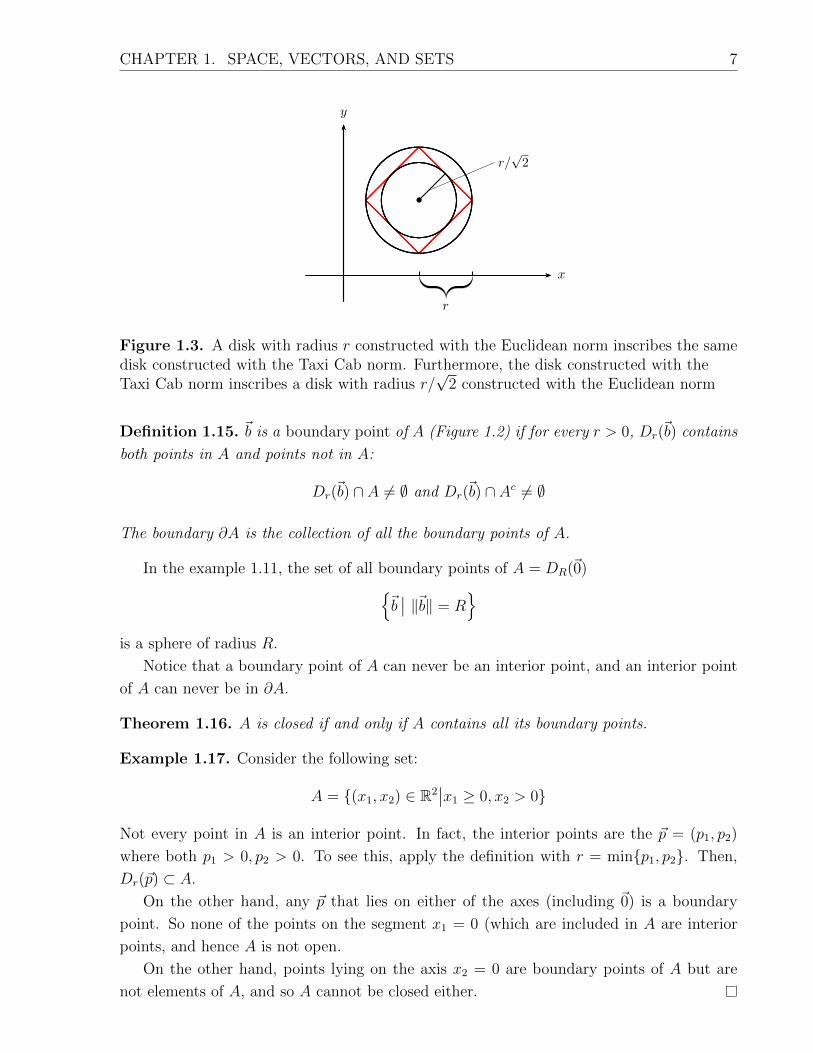
Example 1.12 (Figure 1.3). Suppose we use a Taxi Cab disks instead of a Euclidean disk.
It does not change which points are interior to A since the diamond is inscribed in a circle.
In other words,
Dtaxir (~p) ⊂ DEuclid
r (~p)
Definition 1.13. The complement of set A is
Ac = {~x|~x /∈ A}
That is, Ac consists of all points which are not elements of A. Any point in Rn must
belong either to A or to Ac, but never to both.
Using complements, we define a complementary notion to openness:
Definition 1.14. A set A is closed if Ac is open.
Notice that this does NOT mean that a set A is closed if it is not open. Sets are not
doors: they don’t have to be either open or closed. The open and closed sets are special,
and not every set falls into one of the two categories. Here is a better way of understanding
when a set is closed. First, we define the boundary of a set A:
CHAPTER 1. SPACE, VECTORS, AND SETS 7
x
y
r/√
2
r
Figure 1.3. A disk with radius r constructed with the Euclidean norm inscribes the samedisk constructed with the Taxi Cab norm. Furthermore, the disk constructed with theTaxi Cab norm inscribes a disk with radius r/
√2 constructed with the Euclidean norm
Definition 1.15. ~b is a boundary point of A (Figure 1.2) if for every r > 0, Dr(~b) contains
both points in A and points not in A:
Dr(~b) ∩ A 6= ∅ and Dr(~b) ∩ Ac 6= ∅
The boundary ∂A is the collection of all the boundary points of A.
In the example 1.11, the set of all boundary points of A = DR(~0){~b∣∣ ‖~b‖ = R
}is a sphere of radius R.
Notice that a boundary point of A can never be an interior point, and an interior point
of A can never be in ∂A.
Theorem 1.16. A is closed if and only if A contains all its boundary points.
Example 1.17. Consider the following set:
A = {(x1, x2) ∈ R2∣∣x1 ≥ 0, x2 > 0}
Not every point in A is an interior point. In fact, the interior points are the ~p = (p1, p2)
where both p1 > 0, p2 > 0. To see this, apply the definition with r = min{p1, p2}. Then,
Dr(~p) ⊂ A.
On the other hand, any ~p that lies on either of the axes (including ~0) is a boundary
point. So none of the points on the segment x1 = 0 (which are included in A are interior
points, and hence A is not open.
On the other hand, points lying on the axis x2 = 0 are boundary points of A but are
not elements of A, and so A cannot be closed either.

CHAPTER 1. SPACE, VECTORS, AND SETS 8
1.3 Practice problems
1. Verify that the taxicab norm on R2, ‖~x‖ = |x1| + |x2| satisfies the conditions which
make it a valid norm, that is:
1. ‖~x‖ = 0 if and only if ~x = ~0;
2. ‖a~x‖ = |a| ‖~x‖ for all a ∈ R and ~x ∈ R2;
3. ‖~x+ ~y‖ ≤ ‖~x‖+ ‖~y‖ for all ~x, ~y ∈ R2.
2. (a) Verify that the following identities hold for the Euclidean norm on Rn, defined by:
‖~x‖ =√~x · ~x =
√√√√ n∑j=1
x2j
(i) [Paralellogram Law] ‖~x+ ~y‖2 + ‖~x− ~y‖2 = 2‖~x‖2 + 2‖~y‖2;
(ii) [Polarization Identity] ~x · ~y =1
4
(‖~x+ ~y‖2 − ‖~x− ~y‖2
).
(b) Show that the Parallelogram Law becomes false if we replace the Euclidean norm
on R2 by the Taxicab norm (as defined in problem 1.)
3. Let U = {(x1, x2) ∈ R2 : |x2| ≤ x1, and x1 > 0}. Find all interior points of U and all
boundary points of U . Is U an open set? Is U a closed set?
4. Show each set is open, by showing every point ~a ∈ U is an interior point. [So you need
to explicitly find a radius r > 0 so that Dr(~a) ⊂ U .]
(a) U = {(x1, x2) ∈ R2 : x21 + x22 > 0};
(b) U = {(x1, x2) ∈ R2 : 1 < x21 + x22 < 4}.

Chapter 2
Functions of several variables
2.1 Limits and continuity
In this section, we will be considering vector valued functions such that
F : A ⊆ Rn → Rk.
Using the matrix notation we can write:
F (x1, x2, . . . , xn) =
F1(x1, x2, . . . , xn)F2(x1, x2, . . . , xn)
...Fk(x1, x2, . . . , xn)
.Example 2.1. Given a (k × n) matrix M , we can define the following function:
F (~x) = M~x.
This looks like a pretty special example, but it turns out to be an important one. And it
gives a direct connection between calculus and matrices which we will exploit.
The first order of business is to define what we mean by the limit of a function, and then
we can define the notion of continuity. What does lim~x→~a F (~x) = ~L mean? First, we start
by noting that it is not sufficient to treat each variable, x1, x2, . . . xn, separately.
Example 2.2. Consider the following function:
F (x, y) =xy
x2 + 4y2,
where (x, y) 6= (0, 0).
We can try to find its limit at (0, 0) by treating each variable separately.
limx→0
(limy→0
F (x, y)
)= lim
x→0
(0
x2
)= lim
x→0= 0
9

CHAPTER 2. FUNCTIONS OF SEVERAL VARIABLES 10
Similarly, we have
limy→0
(limx→0
F (x, y))
= 0
However, if we take (x, y) → (0, 0) along a straight line path with y = mx, where m is
constant, we have
F (x,mx) =mx2
x2 + 4m2x2=
m
1 + 4m2
In this case, we have
lim(x,y)→(0,0)along y=mx
F (x, y) =m
1 + 4m2
Therefore, F (x, y) does not approach any particular value as (x, y)→ (0, 0).
We can never show that the limit lim~x→~a F (~x) exists using these kinds of arguments,
but we can show that it does not exist by showing that the limit does not exist along
certain directions, or that it gives different values when approaching ~x→ ~a along different
directions. Thus, we can say that lim~x→~axy
x2+y2does not exist.
Example 2.3. Consider the following function:
F (x, y) =y2
x4 + y2.
If we approach (0, 0) along y = mx, the values of F (x, y) = F (x,mx) → 1. However, if
we approach along a parabola, y = mx2, we obtain a limiting value of m2/(1 + m2). We
get different limits along different parabolas, and so the limit as (x, y) → (0, 0) does not
exist.
From these examples we conclude that if there is to be a limit
lim~x→~a
F (~x) = ~b,
we must have a criterion which doesn’t depend on the path or the direction in which ~x
approaches ~a, but only on proximity. In other words, we want ‖F (~x)−~b‖ to go to zero as
the distance ‖~x− ~a‖ goes to zero, regardless of the path taken in getting there.
Definition 2.4. We say lim~x→~a
F (~x) = ~b if for any given ε > 0, there exists δ > 0 such that
whenever 0 < ‖~x− ~a‖ < δ, we have ‖F (x)−~b‖ < ε. Therefore,
lim~x→~a
F (x) = ~b ⇐⇒ lim~x→~a‖F (~x)−~b‖ = 0
Remark. We can state the definition equivalently in a geometrical form: for any given ε > 0,
there exists a radius δ > 0 such that
F (~x) ∈ Dε(~b),
whenever ~x ∈ Dδ(~a) and ~x 6= ~a.

CHAPTER 2. FUNCTIONS OF SEVERAL VARIABLES 11
Before we look at an example, here’s a useful observations. Take ~v = (v1, v2, . . . , vn) ∈Rn. Then, we have
‖~v‖ =
√√√√ n∑j=1
v2j ≥√v2i = |vi|
for each individual coordinate i = 1, 2, . . . , n. So when applying the definition of the limit,
we may use the following inequalities: for any ~x,~a ∈ Rn,
|xi − ai| ≤ ‖~x− ~a‖, (2.1)
for each i = 1, . . . , n.
Example 2.5. Show
lim(x,y)→(0,0)
2x2y
x2 + y2= 0
Solution: We must set up the definition of the limit. Note that F : R \ {~0} → R, which
is real-valued, so we drop the vector symbols in the range (but not in the domain, which is
R2!) Matching the notation of the definition, we have b = 0, ~a = (0, 0). Call
R = ‖~x− ~a‖ = ‖~x‖ =√x2 + y2,
the distance from ~x to ~a. By the above observation (2.1),
|x| ≤ R, |y| ≤ R.
Since F (~x) ∈ R, the norm ‖F (~x) − ~b‖ = |F (~x) − 0| is just the absolute value. We now
want to estimate the difference |F (~x)− 0| and show that it is bounded by a quantity which
depends only on R, and tends to zero as R→ 0. To do this, we find an upper bound for the
numerator, and a lower bound for the denominator, as a fraction becomes larger when its
numerator is increases, and its denominator is decreased. In this case, the denominator is
exactly R2, and so:
|F (~x)− b| =∣∣∣∣ 2x2y
x2 + y2− 0
∣∣∣∣=
2|x|2|y|x2 + y2
≤ 2 ·R2 ·RR2
= 2R
= 2‖~x− ~a‖
By letting ‖~x−~a‖ = ‖~x‖ < ε/2, we get |F (~x)− 0| < ε. Therefore, the definition is satisfied
by choosing δ > 0 to be any value with 0 < δ ≤ ε/2
CHAPTER 2. FUNCTIONS OF SEVERAL VARIABLES 12
Example 2.6. Consider the following function, F : R3 \ {~0} → R:
F (x, y, z) =3z2 + 2x2 + 4y2 + 6z2
x2 + 2y2 + 3z2, (x, y, z) 6= (0, 0, 0)
Prove that
lim(x,y,z)→(0,0,0)
F (x, y, z) = 2.
Solution: In analogy with the previous example, letR = ‖(x, y, z)−(0, 0, 0)‖ =√x2 + y2 + z2.
We use the “common denominator” to write the desired quantity as a fraction, and estimate
as before:‖F (x, y, z)−~b‖ = |F (x, y, z)− 2|
=
∣∣∣∣3z3 + 2x2 + 4y2 + 6z2
x2 + 2y2 + 3z2− 2
∣∣∣∣=
3|z|3x2 + 2y2 + 3z2
≤ 3R3
x2 + y2 + z2
=3R3
R2
= 3R
Then,
‖F (x, y, z)−~b‖ < 3R < ε
provided that
R = ‖~x−~0‖ < δ =ε
3
Example 2.7. Consider the following function, F : R2 \ {~0} → R:
F (x, y) =(sin3 x)(y + 2)2
[x2 + (y + 2)2]2, (x, y) 6= (0,−2)
Prove that
lim(x,y)→(0,−2)
F (x, y) = 0.
In this example ~a = (0,−2), so the important distance is
R = ‖~x− ~a‖ = ‖(x, y)− (0,−2)‖ =√x2 + (y + 2)2,
that is we want to show that for any ε > 0 we can find δ > 0 so that if 0 < R =
‖(x, y)− (0,−2)‖ < δ, then |F (x, y)− 0| < ε. Notice that
|x| =√x2 ≤
√x2 + (y + 2)2 and |y + 2| =
√(y + 2)2 ≤
√x2 + (y + 2)2,

CHAPTER 2. FUNCTIONS OF SEVERAL VARIABLES 13
and also | sinx| ≤ |x| ≤ R. The denominator is exactly [x2+(y+2)2]2 = ‖~x−(0,−2)‖4 = R4,
and so we may estimate the desired quantity,
|F (x, y)− 0| =∣∣∣∣(sin3 x)(y + 2)2
[x2 + (y + 2)2]2
∣∣∣∣ =| sinx|3|y + 2|2[x2 + (y + 2)2]2
≤ R3R2
R4= R.
Taking δ = ε, if 0 < ‖~x− (0,−2)‖ = R < δ = ε, then |F (x, y)− 0| < ε, as needed.
We are now ready to define continuity. A continuous function is one whose limits coincide
with the value the function at the limit vector:
Definition 2.8. Consider a function F : Rn → Rk with domain A ⊆ Rn. For ~a ∈ A, we
say F is continuous at ~a in the domain of F iff
F (a) = lim~x→~a
F (~x)
Example 2.9. Going back to example 2.6, if we redefine F as follows,
F (x, y, z) =
3z2 + 2x2 + 4y2 + 6z2
x2 + 2y2 + 3z2(x, y, z) 6= (0, 0, 0)
2 (x, y, z) = (0, 0, 0)
then F is continuous at (0, 0, 0) (and at all ~x ∈ R).
If F is continuous at every ~a ∈ A, (∀~x ∈ A), we say F is continuous on the set A.
Continuity is always preserved by the usual algebraic operations: sum. product, quotient,
and composition of continuous functions is continuous.
2.2 Differentiability
You’re used to thinking of the derivative as another function, “derived” from the original
one, which gives numerical values of the rate of change (slope of the tangent line) of the
function. But having a derivative is a property of the function, a measure of how smoothly
the values of the function vary, and so we talk about “differentiability”, the ability of the
function to be differentiated at all.
Let’s recall how the derivative was defined for functions of one variable, because it’s the
basic idea which we’ll return to:
Definition 2.10. For a function f : R→ R, its derivative is defined as
f ′(x) = limh→0
f(x+ h)− f(x)
h.
If it exists, we say f is differentiable at x.
Differentiability is a stronger property than continuity:

CHAPTER 2. FUNCTIONS OF SEVERAL VARIABLES 14
Theorem 2.11. If f : R→ R is differentiable at x, then f(x) is also continuous at x.
Differentiable functions, f(x), are well approximated by their tangent lines (also known
as linearization). We wish to extend this idea to F : Rn → Rm.
First, we can try dealing with independent variables, x1, x2, . . . , xn, one at a time by
using partial derivatives. We start by introducing the standard basis in Rn:
~e1 = (1, 0, 0, . . . , 0)
~e2 = (0, 1, 0, . . . , 0)
...
~en = (0, 0, 0, . . . , 1)
In particular, we have the usual ~e1 =~i, ~e2 = ~j,~e3 = ~k in R3.
For any ~x ∈ Rn, and h ∈ R, (~x + h~ej) moves from ~x parallel to the xj axis by distance
h. In other words,
~x+ h~ej = (x1, x2, . . . , xj + h, xj+1, . . . , xn).
Definition 2.12. A partial derivative of f(x) with respect to xj is defined as
∂f
∂xj(~x) = lim
h→0
f(~x+ h~ej)− f(~x)
h,
for all j = 1, 2, . . . , n (provided the limit exists.)
A partial derivative of function is calculated by treating of ~xj as the only variable, and
all others treated as constants. For a vector valued function F : Rn → Rm,
F (~x) =
F1(~x)F2(~x)
...Fm(~x)
,we treat each component Fi(~x) : Rn → R separately as a real valued function. Each has
n partial derivatives, and so F : Rn → Rm has (m × n) partial derivatives, which form an
(m× n) matrix, the Jacobian matrix or total derivative matrix,
DF (~x) =
(∂Fi∂xj
)i=1,2,...,mj=1,2,...,n
.
Be careful: each row (with fixed i and j = 1, . . . , n) corresponds to the partial derivatives
of one component Fi(~x). Each column (with fixed j and i = 1, . . . ,m) corresponds to
differentiating the vector F (~x) with respect to one independent variable, xj. That is, we
count the components of F top to bottom, and the independent variables’ derivatives left
to right.

CHAPTER 2. FUNCTIONS OF SEVERAL VARIABLES 15
Example 2.13. Consider a function F : R2 → R3:
F (~x) =
x21x1x2x42
.Jacobian of the function is given by
DF (~x) =
∂F1
∂x1
∂F1
∂x2∂F2
∂x1
∂F2
∂x2∂F3
∂x1
∂F3
∂x2
=
2x1 0x2 x10 4x32
The question now is whether the derivative matrix DF (~x) gives us the same information
and properties as the ordinary derivative did in single-value calculus. The following example
shows that we must be more careful with functions of several variables:
Example 2.14. Consider the following function:
f(x, y) =
{xy
(x2+y2)2, (x, y) 6= (0, 0)
0, (x, y) = (0, 0)
Do partial derivatives exist at (0, 0)?
By definition,∂f
∂x(0, 0) = lim
h→0
f(0 + h, 0)− f(0, 0)
h
= limh→0
h·0(h2+02)2
− 0
h
= limh→0
0
h= 0
Similarly, ∂f∂y
(0, 0) = 0 by symmetry of x, y. Therefore,
Df(0, 0) =[0 0
]Although partial derivatives exist, f is not cotinuous at (0, 0). (For example, f(x,mx) →±∞ as x→ 0± for m 6= 0).
By the previous example, we see that the mere existence of the partial derivatives is not
a very strong property for a function of several variables; despite the existence of the partial
derivatives, the function isn’t even continuous at ~x = ~0. So it’s doubtful that the partial
derivatives are giving us very significant information as to the smoothness of the function
in this example. A “differentiable” function should at least be continuous.

CHAPTER 2. FUNCTIONS OF SEVERAL VARIABLES 16
To get a reasonable information from Df(~x), we need to ask for more than just its
existence. To understand what is needed, let’s go back to f : R → R. We rewrite the
derivative at x = a, making the substitution h = x− a in the definition, so that
f ′(a) = limx→a
f(x)− f(a)
x− a .
Equivalently, we have:
0 = limx→a
(f(x)− f(z)
x− a − f ′(x)
)
= limx→a
(f(x)− [
La(x)︷ ︸︸ ︷f(a) + f ′(x)(x− a)]
x− a
)= 0,
where La(x) = f(a) + f ′(x)(x− a) is the linearization of f at a, the equation of the tangent
plane to y = f(x) at x = a. Thus, the difference between the value of f(x) and its tangent
plane La(x) is very small compared to the distance (x − a) of x to a. In other words, f
is differentiable at x if its linear approximation gives an estimate of the value f(x + h) to
within an error which is small compared to ∆x = x− a.
This is the attribute of the one-dimensional derivative which we want to extend to higher
dimensions. Let’s make the analogy. For F : Rn → Rm, F (~x) has (m× n) partial derivates
(see definition 2.12). Then, the linearization of F at ~a is
L~a(~x) = F (~a)︸︷︷︸m×1
+DF (~a)︸ ︷︷ ︸m×n
(~x− ~a︸ ︷︷ ︸n×1
).
So, L : Rn → Rm, just like F . The derivative matrix DF (~a) is a linear transformation of
Rn → Rm.
Notice that when n = 2 and m = 1, For F : R2 → R, we have
DF (~a) =[∂F∂x1
(~a) ∂F∂x2
(~a)],
a (1× 2) row vector and
~x− ~a =
[x1 − a1x2 − a2
],
so we have
L~a(~x) = F (~a) +∂F
∂x1(x1 − a1) +
∂F
∂x2(x2 − a2),
a familiar equation of the tangent plane to z = F (x1, x2).
We’re now ready to introduce the idea of differentiability:
Definition 2.15 (Differentiability). We say F : Rn → Rm is differentiable if
lim~x→~a
‖F (~x)− F (~a)−DF (~a)(~x− ~a)‖‖~x− ~a‖ = 0.

CHAPTER 2. FUNCTIONS OF SEVERAL VARIABLES 17
Equivalently,
lim~h→~0
‖F (~x+ ~h)− F (~x)−DF (~x)~h‖‖~h‖
= 0
In summary, F is differentiable if ‖F (~x) − L~a(~x)‖ is small compared to ‖~x − ~a‖, or if
F (~x) is approximated by L~a(~x) with an error which is much smaller than ‖~x− ~a‖.There is a very useful notation to express this idea that one quantity is very small
compare to another, the “little-o” notation. We write o (h), “little-oh of h”, for a quantity
which is small compred to h., in the sense
g(h) = o(h) ⇐⇒ limh→0
g(h)
h= 0.
Using this notation, differentiability can be written as
‖F (~x)− [F (~a) +DF (~a)(~x− ~a)]‖ = o(‖~x− ~a‖). (2.2)
Example 2.16. Is the following function differentiable at ~a = ~0?
F (x1, x2) =
x22 sinx1√x21+x
22
, ~x 6= ~0
0, ~x = ~0
Solution: First, we have
∂F
∂x1(~0) = lim
h→0
F (~0 + h~e1)− F (~0)
h
= limh→0
0− 0
h= 0
Similarly, we have∂F
∂x2(~0) = 0
So we have
DF (~0) =[∂F∂x1
∂F∂x2
]=[0 0
]For differentiability, we have to look at:∣∣∣∣∣ x22 sinx1√
x21 + x22− 0−
[0 0
]·[x1x2
]∣∣∣∣∣=x22| sinx1|√x21 + x22
Then,|F (~x)− L~0(~x)|‖~x−~0‖
=x22| sinx1|(√x21 + x22
)2 =x22| sinx1|x21 + x22
≤ R2 ·RR2
= R = ‖~x−~0‖

CHAPTER 2. FUNCTIONS OF SEVERAL VARIABLES 18
By the squeeze theorem, we have
lim~x→~0
|F (~x)− L~0(~x)|‖~x−~0‖
= 0
Therefore, F is differentiable at ~x = ~0
Example 2.17. Verify that F is differentiable at ~a = ~0.
F (~x) =
[1 + x1 + x22
2x2 − x21
]First, note that
F (~a) = F (~0) =
[10
]We also need to compute the Jacobian at ~0:
DF (~0) =
[1 00 2
]Then, we get the following linearization of the function:
L~0(~x) = F (~0) +DF (~x)(~x−~0)
=
[10
]+
[1 00 2
] [x1x2
]=
[1 + x1
2x2
]Then, to verify the definition of differentiabiility we estimate the quotient,
‖F (~x)− L~0(~x)‖‖~x−~0‖
=
∥∥∥∥[ x22−x21]∥∥∥∥
‖~x‖ =
√x42 + x41√x21 + x22
≤√R4 +R4
R=√
2R =√
2‖~x−~0‖,
where we have used x41 ≤ R4 and x2 ≤ R4, with R =√x21 + x22.
As ~x → ~0, ‖~x − ~0‖ = R → 0, by the squeeze theorem, the desired limit goes to 0.
Therefore, F is differentiable at ~0.
Verifying differentiability can involve quite a bit of work, but fortunately there is a
powerful theorem which makes differentiability much easier to show.
Theorem 2.18. Suppose F : Rn → Rm, and ~a ∈ Rn. If there exists a disk Dr(~a) in which
all the partial derivatives ∂(Fi(~x))/∂xj exist and are continuous, then F is differentiable at
~x = ~a.
So it’s enough to calculate the partial derivatives and verify that each one is a continuous
function, and then we can conclude that the function is differentiable, without going through
the definition! It’s convenient to give this property a name:

CHAPTER 2. FUNCTIONS OF SEVERAL VARIABLES 19
f is C1
f is differentiable partial derivatives exist
f is continuous
Figure 2.1. Relationship between differentiability and continuity
Definition 2.19. Suppose F : Rn → Rm, and ~a ∈ Rn. If there exists a disk Dr(~a) in
which all the partial derivatives ∂(Fi(~x))/∂xj exist and are continuous, then we say that
F is continuously differentiable, or C1, at ~x = ~a. If F is continuously differentiable at all
points ~x ∈ A, we say that F is continuously differentiable on A, or F ∈ C1(A).
So far as our example, we calculate the partial for ~x 6= ~0:
∂F
∂x1= x22
(cosx1
(x21 + x22
)− 12 +
(−1
2
(x21 + x22
)− 32 2x1
)sinx1
)=
x22(x21 + x22)
3/2
[cosx1
(x21 + x22
)− x1 sinx1
].
This is a quotient of sums, products, and compositions of continuous functions as long as
the denominator is not zero (that is, when (x1, x2) 6= (0, 0),) and therefore it is continuous. I
invite you to calculate ∂F∂x2
, which has a similar form and is also continuous for all (x1, x2) 6=(0, 0). By definition, F is C1 at all ~x 6= ~0, so by Theorem 2.18 we conclude that F is
differentiable at all points in its domain.
We summarize the ideas in this chapter in Figure 2.1. A function which is continously
differentiable is automatically differentiable (by Theorem 2.18.) A function which is dif-
ferentiable must be continuous. However, none of these definitions are equivalent. There
are continuous functions which are not differentiable. There are also functions with partial
derivatives existing but the function is discontinuous. And there are differentiable functions
which are not C1.
2.3 Chain rule
As in single-variable calculus, the composition of differentiable functions is differentiable,
and we have a convenient formula for calculating the derivative.
Let’s be a little careful about domains. Suppose A ⊆ Rn and B ⊆ Rm are open sets,
F : A ⊆ Rn → Rm with F (A) ⊆ B, that is
F (~x) ∈ B for all ~x ∈ A,

CHAPTER 2. FUNCTIONS OF SEVERAL VARIABLES 20
and G : B ⊂ Rm → Rp. Then, we define the composition H : A ⊂ Rn → Rp via
H(~x) = G ◦ F (~x) = G (F (~x)) .
As in single-variable calculus, the composition of continuous functions is continuous:
Theorem 2.20. Let F : A ⊆ Rn → Rm be continuous at ~a ∈ A, and G : B ⊆ Rm → Rp
be continuous at ~b = F (~a) ∈ B. Then the function H = G ◦ F is continuous at ~a.
This is not hard to show, using the δ − ε definition of the derivative, but we leave it for
a later course. Here we are more concerned with differentiation of vector-valued functions.
Example 2.21. This may seem like a overly simple example, but it is an important one.
Consider the case where F and G are linear maps,{F (~x) = M~x M an (m× n) matrix
G(~y) = N~y N an (p×m) matrix
Then,
H(~x) = G (F (~x)) = NM~x
is also a linear function, which is represented by the product NM . (Recall that the order
of multiplication matters a lot!)
In fact this example leads right into the general form of the chain rule for compositions
in higher dimensions. Recall that however nonlinear the functions F and G are, their
derivatives are matrices!
Theorem 2.22. Assume F : Rn → Rm is differentiable at ~x = ~a and G : Rm → Rp is
differentiable at ~b = F (~a). Then, H = G ◦ F is differentiable at ~x = ~a and
DH(~a) = DG(~b)︸ ︷︷ ︸DG(F (~a))
DF (~a)
The product above is matrix multiplication, so be careful of the order of multiplication.
Unless the matrices are both square (which will only happen when the dimensions n = m =
p,) you may not be able to multiply them in the wrong order, but be very careful anyway.
Note that all of the various forms of chain rule done in first year calculus (and explained
by complicated tree diagrams) can be derived directly from this general formula. So the tree
diagrams used in Stewart are just imitating the natural structure of matrix multiplication!
Finally, we point out that the Chain Rule is more than just a formula: it also contains
the information that the composition H = G ◦ F is differentiable at ~a, provided F is
differentiable at ~a and G is differentiable at ~b = F (~a).

CHAPTER 2. FUNCTIONS OF SEVERAL VARIABLES 21
Example 2.23. Consider the following functions, F : R3 → R2 and G : R2 → R2:
F (~x) =
[x21 + x2x3x21 + x23
], G(~y) =
[−y32y1 + y2
]Let H = G ◦ F (~x). Find DH(~a) where ~a = (1,−1, 0).
First, when ~a = (1,−1, 0), ~b = F (~a) = (1, 1). Now,
DF (~x) =
[2x1 x3 x22x1 0 2x3
], DF (1,−1, 0) =
[2 0 −12 0 0
]Similarly, we have
DG(~y) =
[0 −3y21 1
], DG(1, 1) =
[0 −31 1
]As each entry of DF (~x), DG(~y) (the partial derivatives of F,G) is a continuous function
for every ~x, ~y, both F,G are C1 and hence are differentiable, by Theorem 2.18 they are
differentiable. By Chain Rule, we get
DH(1,−1, 0) = DG(1, 1)DF (1,−1, 0)
=
[0 −31 1
] [2 0 −12 0 0
]=
[−6 0 04 0 −1
]
A complete proof of the Chain Rule is a bit complicated, but we can give an idea of why
it works by using the definition of the derivative, written in the form (2.2). Call ~u = F (~x),
for ~x in a neighborhood of ~a. Since G is differentiable at ~b = F (~a), we have
H(~x) = G(F (~x) = G(~u)
= G(~b) +DG(~b) [~u−~b] + E1, (2.3)
with an error E1 = o(‖~u−~b‖). Now, since F is differentiable at ~a, we have
~u−~b = F (~x)− F (~a) = DF (~a) [~x− ~a] + E2, (2.4)
with an error E2 = o(‖~x − ~a‖). This is where we have to be a little tricky: from (2.4) we
do two things. The first is that E1 = o(‖~u−~b‖) = o(‖~x− ~a‖) is also small compared with
‖~x− ~a‖, and the second is that we can substitute into (2.3) to obtain:
H(~x) = G(~b) +DG(~b) [DF (~a) (~x− ~a) + E2] + E1
= H(~a) +DG(~b)DF (~a) (~x− ~a) + o(‖~x− ~a‖),
that is,
H(~x)−H(~a)−DG(~b)DF (~a) (~x− ~a) = o(‖~x− ~a‖).By the definition of the derivative, H is differentiable at ~a, with Jacobian (total derivative)
given by the matrix product, DH(~a) = DG(~b)DF (~a).

CHAPTER 2. FUNCTIONS OF SEVERAL VARIABLES 22
2.4 Practice problems
1. Prove each of the following using the definition of the limit. (To show the limit does
not exist, it is enough to consider the limit along different paths.)
(a) lim~x→~0
x61x61 + 3x22
does not exist.
(b) lim~x→~0
x31x22
[x21 + x22]2
= 0.
(c) lim~x→(1,2)
(x1 − 1)2(x2 − 2)2
[(x1 − 1)2 + (x2 − 2)2]32
= 0
2. Let F (x, y) =xy2
(x2 + y2)2for (x, y) 6= (0, 0) and f(0, 0) = 0.
(a) Show that∂f
∂x(0, 0),
∂f
∂y(0, 0) both exist.
(b) Show that f is not continuous at (0, 0).
3. Let M be a k × n matrix, and define F (~x) = M~x (ie, via matrix multiplication, with ~x
as a column vector.) Use the definition of differentiability to show that F is differentiable
at all ~x ∈ Rn, and DF (~x) = M .
4. Let F : R2 → R3 be defined by
F (~x) =
x1 cosx2x1x
22
e−x2x1
Find DF (~x). Calculate the linearization L~a(~x) around ~a = (1, 0).
5. Let F : R2 → R2, G : R2 → R2, defined by
F (r, θ) =
[r cos θr sin θ
], G(x, y) =
[2xy
y2 − x2]
and let H = G ◦ F . Explain why F , G, and H are all differentiable, and use the chain rule
to calculate DH(√
2, π4).
6. Justify the approximation
ln(1 + 2x1 + 4x2) = 2x1 + 4x2 + o(‖~x‖)
for ~x close to ~0.

Chapter 3
Paths, directional derivative, andgradient
In this section we use the chain rule to explore two very common (and complementary)
situations,
• parametrized paths, ~c : R→ Rn, for which the domain is one-dimensional;
• real-valued f : Rn → R, which are functions of n ≥ 2 variables but are scalar-valued.
In fact, we will use paths as a tool to derive some qualitative facts about functions of several
variables.
3.1 Paths and curves
We start with paths, which parametrize curves in Rn. First, recall that an interval is a
connected set in the real line, which includes the open intervals (a, b), (−∞, b), (a,∞),
or (−∞,∞) = R; the closed intervals [a, b], [a,∞), (−∞, b] (which include endpoints); or
intervals like (a, b] which are neither open nor closed.
Definition 3.1. Let I ⊆ R be an interval. A path ~c : I ⊆ R → Rn is a vector-valued
function of a scalar independent variable, usually, t:
~c(t) =
c1(t)c2(t)
...cn(t)
The path ~c(t) can be thought of as a vector (or a point, representing the tip of the
vector) moving in time t. The moving point traces out a curve in Rn as t increases, and
thus we use paths to attach functions (the moving coordinates) to a geometrical object, a
curve in space. Note that this is not the only way to describe a curve:
23

CHAPTER 3. PATHS, DIRECTIONAL DERIVATIVE, AND GRADIENT 24
Example 3.2. A unit circle in R2 described as a path is
~c(t) = (cos t, sin t),
where t ∈ [0, 2π). But we could also describe the unit circle non-parametrically as
x2 + y2 = 1
We will talk about such non-parametric curves and surfaces in a later chapter.
Note that the same curve can be described by different paths. Going back to unit circle,
we can also write~b(t) =
(sin(t2), cos(t2)
), t ∈ [0,
√2π).
Using different paths can change (1) time dynamics and (2) direction of the curve. This
curve has a non-constant speed and reversed orientation, that is, the path ~c(t) traces the
circle counter-clockwise while ~b(t) draws it clockwise.
If ~c is differentiable, D~c(t) is an (n×1) matrix. Since each component ~cj(t) is a real-valued
function of only one variable, the partial-derivative is the usual (or ordinary) derivative:
∂cj∂t
=dcjdt
= c′j(t) = limh→0
cj(t+ h)− cj(t)h
So D~c(t) = ~c ′(t) is written as a column vector:
D~c(t) =
c′1(t)c′2(t)
...c′3(t)
= lim
h→0
~c(t+ h)− ~c(t)h
which is a vector which is tangent to the curve traced out at ~x = ~x(t). Physically, ~c ′(t) is
the velocity vector for motion along the path (Figure 3.1).
Example 3.3 (Lines). Given two points, ~p1, ~p2 ∈ Rn, there is a unique line connecting
them. One path which represents this line is
~c(t) = ~p1 + t~v,
where ~v = ~p2 − ~p1. Velocity is then given by ~c ′(t) = ~v, a constant.
A path, ~c(t), is continuous (or differentiable, or C1,) provided that each of the compo-
nents cj(t), j = 1, 2, . . . , n is continuous (or differentiable, or C1.) Note that {~c(t) : t ∈ [a, b]}traces out a curve in Rn, with initial endpoint, ~a, and final endpoint, ~b. The path ~c(t) pa-
rameterizes the curve drawn out.
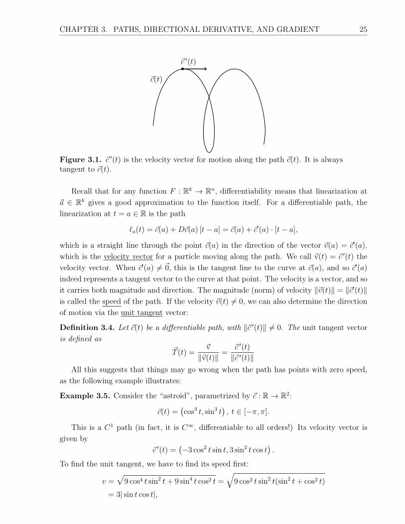
CHAPTER 3. PATHS, DIRECTIONAL DERIVATIVE, AND GRADIENT 25
~c ′(t)
~c(t)
Figure 3.1. ~c ′(t) is the velocity vector for motion along the path ~c(t). It is alwaystangent to ~c(t).
Recall that for any function F : Rk → Rn, differentiability means that linearization at
~a ∈ Rk gives a good approximation to the function itself. For a differentiable path, the
linearization at t = a ∈ R is the path
`a(t) = ~c(a) +D~c(a) [t− a] = ~c(a) + ~c′(a) · [t− a],
which is a straight line through the point ~c(a) in the direction of the vector ~v(a) = ~c′(a),
which is the velocity vector for a particle moving along the path. We call ~v(t) = ~c ′(t) the
velocity vector. When ~c′(a) 6= ~0, this is the tangent line to the curve at ~c(a), and so ~c′(a)
indeed represents a tangent vector to the curve at that point. The velocity is a vector, and so
it carries both magnitude and direction. The magnitude (norm) of velocity ‖~v(t)‖ = ‖~c′(t)‖is called the speed of the path. If the velocity ~v(t) 6= 0, we can also determine the direction
of motion via the unit tangent vector:
Definition 3.4. Let ~c(t) be a differentiable path, with ‖~c ′(t)‖ 6= 0. The unit tangent vector
is defined as
~T (t) =~v
‖~v(t)‖ =~c ′(t)
‖~c ′(t)‖All this suggests that things may go wrong when the path has points with zero speed,
as the following example illustrates:
Example 3.5. Consider the “astroid”, parametrized by ~c : R→ R2:
~c(t) =(cos3 t, sin3 t
), t ∈ [−π, π].
This is a C1 path (in fact, it is C∞, differentiable to all orders!) Its velocity vector is
given by
~c ′(t) =(−3 cos2 t sin t, 3 sin2 t cos t
).
To find the unit tangent, we have to find its speed first:
v =√
9 cos4 t sin2 t+ 9 sin4 t cos2 t =√
9 cos2 t sin2 t(sin2 t+ cos2 t)
= 3| sin t cos t|,

CHAPTER 3. PATHS, DIRECTIONAL DERIVATIVE, AND GRADIENT 26
c(t) = (cos3 t, sin3 t)
T (t)
Figure 3.2. For ~c(t) = (cos3 t, sin3 t), unit tangent suddenly changes its direction at thecusp.
remembering that√x2 = |x|, because we always choose the positive square root. Then, the
unit tangent is given by
~T (t) =~v(t)
‖~v(t)‖ =
(−| cos t| sin t
| sin t| , | sin t|cos t
| cos t|
)Note that its tangent is undefined when sin t = 0 or cos t = 0, i.e. at multiples of π
2.
Worse, sin t| sin t| ,
cos t| cos t| flip discontinuously as t crosses a multiple of π/2 from −1 to +1, or vice
versa. Although the path is C1, the curve is not smooth! When ~v(t) = ~c ′(t) = 0, it allows
the curve to have cusps (Figure 3.2).
Note that it is possible to have a nice tangent direction even when ~c ′(t) = 0:
Example 3.6. For constant vectors ~p, ~w 6= ~0 in Rn, define the two paths
~c(t) = ~p+ ~wt2, t ∈ R,~b(t) = ~p+ ~wt3, t ∈ R.
Each is continuously differentiable for all t ∈ R. First, ~c′(t) = 2t~w, with speed ‖~c′(t)‖ =
2|t| ‖~w‖. The unit tangent vector,
~T (t) =2t~w
2|t| ‖~w‖ =
{+ ~w‖~w‖ , if t > 0,
− ~w‖~w‖ , if t < 0,
and is undefined at t = 0. Notice that ~c(t) traces out a half-line, starting at t = 0 at the
point ~c(0) = ~p, and moving along the ray in the direction of positive multiples of ~w, for
t < 0. When t < 0 it moves along the same line, but in the opposite direction, towards ~p as
t→ 0−. The path is not smooth, since velocity is zero at t = 0, and the unit tangent jumps
at that time.
The path ~b(t) is also not smooth, since ~b′(0) = ~0. But the difficulty here is artificial:~b′(t) = 3t2 ~w, with speed ‖~b′(t)‖ = 3t2‖~w‖. Although the speed is also zero at t = 0, we can
still define a unit tangent vector, ~T (t) = ~w‖~w‖ when t 6= 0 has a removable discontinuity. It’s
simply a bad choice to parametrize the line; the curve (straight line) is smooth even though
the path ~b(t) is not!

CHAPTER 3. PATHS, DIRECTIONAL DERIVATIVE, AND GRADIENT 27
Although it’s possible to have a continuously varying tangent vector even when the
speed of the path can vanish, we wish to avoid such tricky cases. So we will only call a
curve “smooth” if the speed is never zero, and so the unit tangent ~T (t) may be defined, and
will be continuous:
Definition 3.7. We say a path ~c(t), t ∈ I, is smooth (or regular) if ~c is a C1 path with
‖~c ′(t)‖ 6= 0 for any t ∈ I. We call a geometrical curve smooth if can be parametrized by a
C1 path ~c(t) which is smooth (ie, C1 with nonvanishing speed.)
For a smooth curve the unit tanget vector ~T (t) is continuous, and so we eliminate the
bad behavior of the astroid example above.
Specializing to curves in space ~c(t) ∈ R3, we will want to use vector operations to study
the velocity and tangent vectors associated to the paths. The following product rules will
be useful:
Theorem 3.8.
1. If f : R→ R, ~c : R→ Rn, both differentiable,
d
dt
(f(t)~c(t)
)= f(t)~c ′(t) + f ′(t)~c(t)
2. If ~c, ~d : R→ Rn are differentiable,
d
dt
(~c(t) · ~d(t)
)= ~c ′(t) · ~d(t) + ~c(t) · ~d ′(t)
3. If ~c, ~d : R→ R3 are differentiable,
d
dt
(~c(t)× ~d(t)
)= ~c(t)× ~d ′(t) + ~c ′(t)~d(t),
where ~c× ~d =∑3
i,j,k=1 cidj~ekεijk1.
To prove these, we write them in components,
~c(t) = (c1(t), c2(t), . . . , cn(t)) =n∑i=j
cj ~ej,
1 εijk =
0 if i = j or j = k or k = i
1 if (i, j, k) is positively ordered
−1 if (i, j, k) is negatively ordered

CHAPTER 3. PATHS, DIRECTIONAL DERIVATIVE, AND GRADIENT 28
using the standard basis {~e1, . . . , ~en} of Rn, and do the ordinary derivative. For example,
d
dt
(f(t)~c(t)
)=
d
dt
( n∑j=1
f(t)~cj(t)~ej
)=
n∑j=1
d
dt
(f(t)~cj(t)
)~ej
=n∑j=1
(f ′(t)~cj(t) + f(t)~cj
′(t))~ej
= f ′(t)~c(t) + f(t)~c ′(t).
The verification of the other two formulae are left as an exercise.
Example 3.9. Suppose ~c is a twice differentiable path and its acceleration vector ~a(t) =
~c′′(t) satisfies the equation
~a(t) = k~c(t)
for some constant k 6= 0. Show that ~c(t) describes a motion in a fixed plane.
Define a vector,
~n(t) = ~c(t)× ~v(t) = ~c(t)× ~c ′(t).
Notice ~n(t) ⊥ ~c(t) and ~n(t) ⊥ ~v(t), i.e. ~n(t) is normal to the plane containing the vectors
~c,~v (drawn with common endpoint.) Our goal is to show that ~n is a constant, independent
of t, in which case the path ~c(t) always lies in the same plane which is normal to ~n. To do
this, we differentiate the equation defining ~n,
d~n
dt=
d
dt(~c(t)× ~c ′(t)) = ~c(t)× ~c ′′(t)︸ ︷︷ ︸
~a(t)
+~c ′(t)× ~c ′(t)︸ ︷︷ ︸~0
= ~c(t)× k~c(t)= ~0
Therefore, ~n is constant in time.
As ~n is a constant vector, it defines a fixed plane,
P = {~w | ~w · ~n = 0}
passing through the origin, which contains the moving vector ~c(t) for all t. We have just
shown that the path moves in the plane P .
Definition 3.10 (Arc length). The arc length (or distance traveled along the parameterized
curve) for a ≤ t ≤ b is given by ∫ b
a
‖~c ′(t)‖︸ ︷︷ ︸speed
dt

CHAPTER 3. PATHS, DIRECTIONAL DERIVATIVE, AND GRADIENT 29
We are also interested in keeping track of how much distance we travel along a path,
starting at a fixed time t = a. Think of the trip odometer in a car, which you set to zero at
the start of a road trip and keeps track of how far you’ve driven since you started out.
Definition 3.11 (Arc length function). The arc length function associated to the path ~c(t),
with starting time t = a is
s(t) =
∫ t
a
‖~c ′(u)‖du
We use the dummy variable u in the integral since the independent variable t is one of
the limits of integration. So the arclength function s(t) is an antiderivative of the speed
‖~c ′(t)‖,ds
dt= ‖~c ′(t)‖,
but with the constant of integration chosen to make s(0) = 0. If this seems mysterious, you
should review the First Fundamental Theorem of Calculus from Stewart.
Example 3.12. Consider the following path:
~c(t) = (3 cos t, 3 sin t, 4t), t ∈ [0, 4π].
Its velocity vector is given by
~v(t) = (−3 sin t, 3 cos t, 4).
It follows that its speed ‖~c ′(t)‖ =√
32 + 42 = 5. Then, we can compute the arc length
function:
s(t) =
∫ t
0
v(t)dt =
∫ t
0
5du = 5t
In particular, the total arc length over t ∈ [0, 4π] is s(4π) = 20π.
Definition 3.13. When the path ~c(t) traces out the curve with speed ‖~v(t)‖ = 1 for all t,
we say that the curve is arc length parameterized.
We note that a C1 arclength parametrized path is smooth. If a curve is arc length
parameterized, its arc length function becomes
s(t) = t
In this case it is conventional to use the letter s instead of t as the parameter in the path.
Theorem 3.14. Let ~c(t), t ∈ I, be a smooth path. Then, there is an arclength reparametriza-
tion for the curve, ~γ(s), with ‖~γ′(s)‖ = 1 for all s.
Example 3.15. In example 3.12, the helix is not arc length parameterized but we can re-
parameterize it so that it is. To do so, we need to solve for t = ϕ(s) to invert the function,
s(t).
Going back the example, we had s(t) = 5t. It follows that t = 15s. Then,
~c(s) = ~c(ϕ(s)) = ~c(s
5
)=
(3 cos
(s5
), 3 sin
(s5
),4s
5
)is an arc length parameterization of the original helix, i.e. ‖~c ′(s)‖ = 1, ∀s.

CHAPTER 3. PATHS, DIRECTIONAL DERIVATIVE, AND GRADIENT 30
3.2 Directional derivatives and gradient
Now let’s use curves to explore functions defined on Rn. We restrict our attention here to
real (scalar) valued functions, that is f : Rn → R. Think of f(~x) as describing a quantity
such as temperature or air pressure in a room, and an insect or drone moving around the
room along the path ~c(t), measuring the value of f as it moves. In other words, it measures
the composition, h(t) = f(~c(t)).
If f : Rn → R is differentiable, Df(~x) is a (1× n) matrix:
Df(~x) =[∂f∂x1
∂f∂x2
· · · ∂f∂xn
]We use paths ~c(t) to explore f(x) by looking at
h(t) = f ◦ ~c(t) = f (~c(t)) .
where h : R→ R, By chain rule,
Dh(t) = h′(t) = Df(~c(t))︸ ︷︷ ︸1×n
D~c(t)︸ ︷︷ ︸n×1
= Df (~c(t))~c ′(t)
=[∂f∂x1
∂f∂x2
· · · ∂f∂xn
]c′1c′2...c′n
We can think of this as a dot product of ~c ′(t) with a vector DfT = ∇f , the gradient vector:
h′(t) = ∇f(~c(t)) · ~c ′(t)
Suppose f : Rn → R is differentiable at ~a ∈ Rn, and we have a path ~c : Rn → R with
~c(0) = ~a. Let ~v = ~c ′(0). Then, h′(0) measures rate of change of f along the path, ~c, as we
cross through ~a:
h′(0) = ∇f(~c(0)) · ~c ′(0)
= ∇f(~c(0)) · ~vNote that we get the same value for h′(0) for any path ~c(t) going through ~a with velocity
~c ′(0) = ~v: other than insisting that the path pass through the point ~a with velocity vector
~v, this quantity is path-independent. In other words, h′(0) says something about f at ~a,
and not the past or future trajectory of the path ~c(t). In particular, we get the same value
for the derivative h′(0) if we take the simplest possible path which passes through ~a with
velocity ~v at t = 0, a straight line,
~c(t) = ~a+ t~v, t ∈ R.

CHAPTER 3. PATHS, DIRECTIONAL DERIVATIVE, AND GRADIENT 31
When we use the straight line to calculate h′(0), it means that we can write h(t) = f(~c(t)) =
f(~a+ t~v), and so
h′(0) = limt→0
h(t)− h(0)
t− 0= lim
t→0
f(~a+ t~v)− f(~a)
t.
This is an important quantity to calculate for any function f , and so we give it a name:
Definition 3.16 (Directional derivative). The directional derivative of f at ~a in direction
~v is given by
D~vf(~a) = limt→0
f(~a+ t~v)− f(~a)
t.
If the function f is differentiable at ~a, then we may apply the chain rule as above and
obtain:
Theorem 3.17. Let f : Rn → R be differentiable at ~x = ~a, and ~v ∈ Rn a nonzero constant
vector. Then,
D~vf(~a) =d
dtf(~a+ t~v)
∣∣t=0
= ∇f(~a) · ~v.
Now, we can make some observations. Since the shape of the path ~c(t) doesn’t matter,
only that it passes through ~a with velocity ~v, we might as well choose a straight line path
when calculating directional derivatives, ~c(t) = ~a + t~v, with ~c(0) = ~a and ~c′(0) = ~v. Using
the Chain Rule as above, the directional derivative can be rewritten as
D~vf(~a) = Df(~a)~v = ∇f(~a) · ~v.
From this formula we recognize that the partial derivatives are just special cases of direc-
tional derivatives, obtained by choosing ~v = ~ej. That is,
∂f
∂xj(~a) = D~ejf(~a).
There is one little problem with our definition of directional derivatives: D~vf(~a) depends
not only on the “direction” of the vector ~v, but also its magnitude. To see this, notice that
although ~v and 2~v are parallel (and thus have the same direction,) D2~vf(~a) = ∇f(~a) ·(2~v) =
2D~vf(~a). To get the information on how fast f is changing at ~a, we need to restrict to unit
vectors ‖~v‖ = 1. So we often use the term “directional derivative” only when ~v is a unit
vector.
Directional derivatives also give a geometrical interpretation of the gradient vector,
∇f(~a), when ∇f(~a) 6= ~0. Applying the Cauchy-Schwartz inequality (Theorem 1.2), we
have:
|D~vf(~a)| = |∇f(~a) · ~v| ≤ ‖∇f(~a)‖‖~v‖ = ‖∇f(~a)‖,and equality holds if and only if ~v is parallel to ∇f(~a). Therefore, we can conclude that
the length of the gradient vector, ‖∇f(~a)‖, gives the largest of D~vf(~a) among all choices of
unit directions ~v,
‖∇f(~a)‖ = max {D~uf(~a) : ~u ∈ Rn with ‖~u‖ = 1} .

CHAPTER 3. PATHS, DIRECTIONAL DERIVATIVE, AND GRADIENT 32
In other words, the direction ~v in which f(~x) increases most rapidly is the direction of
∇f(~a), i.e.
~v =∇f(~a)
‖∇f(~a)‖ ,
provided that ∇f(~a) 6= ~0.
Similarly, −∇f(~a) points in the direction of the least (most negative) D~vf(~a), i.e.
~v = − ∇f(~a)
‖∇f(~a)‖ ,
gives the direction in which f decreases fastest at ~a.
3.3 Gradients and level sets
We recall that if G : Rn → R, the level set of G at level k ∈ R (a constant) is
S = {~x ∈ Rn : G(~x) = k}.
For example, in R2, the function f(x, y) = x2 + y2 has level sets x2 + y2 = k which define
circles of radius√k when k > 0. When k = 0 the level set consists only of the origin, and
for k < 0 the level set is empty, S = ∅. This suggests that generically (that is, for all but
a few values of k,) when it is non-empty the level set of a C1 function of 2 variables is a
curve, but that it can be lower dimensional (a point.) (Later on, with the Implicit Function
Theorem we will understand why this is so.)
What does the gradient ∇G tell us in this situation? The graph of G(~x) lies in the
higher dimensional space Rn+1, and so when n ≥ 3 we can’t really visualize the graph.
However, we know from the last section that G increases most rapidly if we move ~x along
the direction of ∇G(~x). Moving ~x along the level set S doesn’t change the value of G at
all, so this suggests that the directional derivatives “along” the level set are zero.
A more precise description uses the concept of the tangent plane to the surface. As we
did in the last section, we use paths ~c(t) to explore the surface (or curve, in 2D) defined by
the level set. To do this, we only consider smooth paths ~c(t) which remain on the surface
S for all time t ∈ R. Since “remaining on the surface” means that the coordinates of
~c(t) = (x1(t), . . . , xn(t)) must solve the equation G(~x) = k at all times, we have
G(~c(t)) = k, ∀t ∈ R.
Taking such a path, assume it passes through the point ~a ∈ S at time t = 0, with velocity
vector ~v = ~c ′(0). Then, ~v must be a tangent vector to the surface S at the point ~a ∈ S. In
fact, this is how we define a tangent plane (or tangent line, in 2D) to the surface S, as the
collection of all possible velocity vectors corresponding to paths lying along the surface S.
Using implicit differentiation and the chain rule, since G(~c(t)) = k is constant,
0 =d
dt(k) =
d
dtG(~c(t)) = ∇G(~c(t)) · ~c′(t). (3.1)

CHAPTER 3. PATHS, DIRECTIONAL DERIVATIVE, AND GRADIENT 33
Evaluating at t = 0, we get
∇G(~a) · ~v = 0,
so the vector ∇G(~a) is orthogonal to the tangent vector ~v. Since this is true for any path
~c(t) with any velocity vector ~v, it follows that ∇G(~a) is either the zero vector or it is a
normal vector to the plane containing all tangent vectors.
Theorem 3.18. Assume G : Rn → R is a C1 function, ~a ∈ Rn, k = G(~a), and S = {~x ∈Rn : G(~x) = k} is the level set.
If ∇G(~a) 6= ~0, then ∇G(~a) is a normal vector to the tangent plane of S at ~a.
Example 3.19. Suppose g : R → R is C1 with g′(r) 6= 0 for all r > 0, and G : R3 → Ris defined by G(x, y, z) = g(x2 + y2 + z2). If the orgin does not lie on the level set S =
{(x, y, z) : G(x, y, z) = k}, then its normal vector is parallel to the vector ~x = (x, y, z).
To see this, use the chain rule to calculate the gradient of G: define r = f(x, y, z) =
x2 + y2 + z2, and then
DG(x, y, z) = Dg(r)Df(x, y, z) = [g′(r)][2x 2y 2z
]= 2g′(r)
[x y z
]Writing this as a gradient vector, ∇G = 2g′(r)~x, which is parallel to ~x as long as g′(r) 6= 0,
which is true since the origin (r = 0) does not lie on the level set.
3.4 Lagrange multipliers
As an application of these ideas we present the method of Joseph-Louis Lagrange (1736-
1813) for finding constrained maxima and minima. Here’s the setup: we want to minimize
or maximize a function F : Rn → R, but only over those vectors which satisfy a constraint
condition, given as the level set of G : Rn → R. That is, we want to
maximize (or minimize) F (~x) for all ~x with G(~x) = k, (3.2)
where k is a fixed constant. Such optimization problems arise naturally in fields such as
economics, where fixed resources or capacities restrict our choice when optimizing.
The way that Lagrange solves this problem is to introduce a new unknown scalar λ, the
“Lagrange multiplier”, into the problem:
Theorem 3.20 (Lagrange multipliers). Assume F,G : Rn → R are C1 functions. If the
constrained optimization problem (3.2) is attained at ~x = ~a, and ∇G(~a) 6= ~0, then there is
a constant λ ∈ R with
∇F (~a) = λ∇G(~a).
Proof of Theorem 3.20. Assume F has a maximum at ~a ∈ S, that is, with G(~a) = k.
Consider any path ~c(t) which lies on the surface S and passes through ~a, so G(~c(t)) = k is
constant for all t, with ~c(0) = ~a and ~c′(0) = ~v is a tangent vector to S at ~a. The function

CHAPTER 3. PATHS, DIRECTIONAL DERIVATIVE, AND GRADIENT 34
h(t) = F (~c(t)) has its maximum at t = 0 (when ~c(0) = ~a,) and so by first year calculus
h′(0) = 0. As in the derivation of (3.1), by implicit differentiation and the chain rule we
have
0 = h′(0) = ∇F (~c(0)) · ~c′(0) = ∇F (~a) · ~v,
for any tangent vector ~v to S at ~a. In other words, ∇F (~a) is orthogonal to all of the vectors
in the tangent plane to S, so it must point parallel to the normal vector of S. But by
Theorem 3.18 that is given by ∇G(~a), and so there is a constant λ of proportionality for
which ∇F (~a) = λ∇G(~a).
So the gradients of F andG are parallel at a solution of the constrained extremal problem.
Geometrically, since ∇F (~a) is a normal vector to the level set of F , and similarly ∇G(~a) is
a normal vector to the constraint set S (which is a level set of G), a maximum or minimum
value of F on S where a level set of F is tangent to the constraint set S. See Figure 3.3
below.
In practice, this means solving a system
∇F (~x) = λ∇G(~x), G(~x) = k, (3.3)
with (n + 1) equations in the (n + 1) unknowns, ~x = (x1, . . . , xn) and λ, for the (n + 1)
unknowns ~x = (x1, . . . , xn) and λ. This may be a linear system, but in most cases it will be
nonlinear. So typically, Gaussian elimination is not applicable and we must be clever and
crafty to combine the equations and hope to be able to find the solutions.
Notice what the Theorem does not say: it does not say that there must exist points
where the maximum or minimum of F on the surface S = {~x | G(~x) = k}. Nor does it
exclude the possibility that the maximum and/or minimum occurs at points where F or G
fails to be C1 or even at points where ∇G(~a) = ~0. So our best hope is to find the solutions
to the Lagrange Multiplier equation (3.3), check if there are any points on S with ∇G = ~0,
and reason out whether they are minima or maxima (or neither!) We are aided by the
following fact (which you encountered in first year calculus):
Theorem 3.21. Let F : Rn → R be a continuous function, and S ⊂ Rn be a set which is
both closed and bounded. Then F (~x) attains both its maximum and minimum values on the
set S.
The case f : R→ R is continuous on the closed and bounded interval [a, b] is in Stewart,
p. 278 in Chapter 4 (the “Extreme Value Theorem”.) If the constraint set is unbounded
we may not have a maximum or minimum value at all.
Example 3.22. Find the closest and furthest point from the origin to the surface 4x2 +
2xy + 4y2 + z2 = 1.
First we need to set this up as a problem with level set constraint. The function to be
optimized is the distance to the origin, which is ‖~x‖. However, it is equivalent (and much
CHAPTER 3. PATHS, DIRECTIONAL DERIVATIVE, AND GRADIENT 35
easier) to instead minimize/maximize the square of the distance, F (~x) = ‖~x‖2 = x2+y2+z2,
since the square is a monotone increasing function of positive numbers. The constraint is
G(x, y, z) = 1, with G(x, y, z) = 4x2 + 2xy + 4y2 + z2. These are C1 functions, so by
Theorem 3.2 at an extrema we must satisfy the equations (3.3), which in this example
gives:
2x = λ(8x+ 2y), 2y = λ(2x+ 8y), 2z = 2λz, 4x2 + 2xy + 4y2 + z2 = 1,
to be solved for (x, y, z) and λ. Note that these equations are nonlinear, but with a bit of
care we will use linear algebra anyway. But be very careful not to let solutions go unnoticed!
The easiest equation is the third one, 2z = 2λz or (1 − λ)z = 0. So there are two
possibilities (both of which must be dealt with!) z = 0 or λ = 1. First, assume z = 0 . We
rewrite the first two equations as a system,4x+ y =
1
λx
x+ 4y =1
λy
or, equivalently,
(
4− 1
λ
)x+ y = 0
x+
(4− 1
λ
)y = 0.
If this looks familiar it’s because it’s an eigenvalue problem (except the eigenvalue is called
1/λ.) To find a nonzero solution we need the determinant of the matrix of coefficients to
vanish (as in the eigenvalue problem!), that is
0 = det
[(4− 1
λ
)1
1(4− 1
λ
)] =
(4− 1
λ
)2
− 1 =
(5− 1
λ
)(3− 1
λ
).
So we can solve for λ = 15, 13; that is, there are two different possibilites for λ when z = 0.
When λ = 15, substituting into the first equation of the system gives y = x. Then, plugging
into the constraint equation,
1 = 4x2 + 2xy + 4y2 + z2 = 4x2 + 2x2 + 4x2 + 0 = 10x2,
and so x = ±√
110
. This gives our pair of solutions to the equations,
(x, y, z) =
(√1
10,
√1
10, 0
), (x, y, z) =
(−√
1
10,−√
1
10, 0
).
(Be careful: since y = x we don’t get all the permutations of the signs!) For the other
Lagrange multiplier λ = 13, we again use the first equation to get y = −x, and then the
constraint gives us
1 = 4x2 + 2xy + 4y2 + z2 = 4x2 − 2x2 + 4x2 + 0 = 6x2,
and so x = ±√
16. This gives our pair of solutions to the equations,
(x, y, z) =
(√1
6,−√
1
6, 0
), (x, y, z) =
(−√
1
6,
√1
6, 0
).

CHAPTER 3. PATHS, DIRECTIONAL DERIVATIVE, AND GRADIENT 36
This exhausts all the possibilites for the case z = 0.
The other case was λ = 1, in which case the equations for (x, y) become
3x+ y = 0 x+ 3y = 0,
which has only the trivial solution (x, y) = (0, 0) (check the determinant of the coefficient
matrix!) Plugging into the constraint,
1 = 4x2 + 2xy + 4y2 + z2 = 0 + 0 + 0 + z2 = 1,
so z = ±1, and we get
(x, y, z) = (0, 0, 1), (x, y, z) = (0, 0,−1).
Thus, we have 6 points which satisfy the Lagrange multiplier equations. The maximum and
minimum must be attained among these, so test them in F (x, y, z):
F
(±(√
1
10,
√1
10, 0
))=
1
5, F
(±(√
1
6,−√
1
6, 0
))=
1
3, F (0, 0,±1) = 1.
The minimum value is 15, attained at the points (x, y, z) = ±
(√110,√
110, 0)
, and the
maximum value is 1, attained at the points (x, y, z) = (0, 0,±1).
Example 3.23. Find the point on S = {(x, y) ∈ R2 | x2y = 2} which is closest to (0, 0).
As in the above example, the function which we wish to optimize is F (x, y) = ‖(x, y)−(0, 0)‖2 = x2 + y2, as the square of the distance is minimized (or maximized) whenever the
distance is. The constraint G(x, y) = x2y has level sets which may be expressed as graphs
in the plane, y = k/x2, x 6= 0, when k 6= 0. The level sets are not closed curves, and are
unbounded sets, and hence we are not guaranteed to have either maximum or minimum
values of F (x, y) for given functions F . In particular, for this choice F (x, y) = x2 + y2,
there can be no maximum value, since (x, 2x−2) ∈ S for each x 6= 0, and F (x, 2x−2) =
x2 + 4x−4 −→ +∞ diverges as x→ 0.
Let’s see if we can find a minimum value, which seems to exist given the graph in
Figure 3.3 below. We seek solutions to the Lagrange Multiplier equations, (3.3),
∇F (x, y) = (2x, 2y) = λ∇G(x, y) = λ(2xy, x2
).
That is,
2x = 2λyx, 2y = λx2, x2y = 2.
The first equation gives us x(1 − λy) = 0, so either x = 0 or 1 − λy = 0. Since x = 0
is impossible (we can’t satisfy the constraint!) we must have y = 1/λ. From the second
equation, 2λ
= λx2, or x2 = 2/λ2. Now we plug this into the constraint,
2 = x2y =
(2
λ2
)(1
λ
)=
2
λ3,

CHAPTER 3. PATHS, DIRECTIONAL DERIVATIVE, AND GRADIENT 37
and so λ = 1 is the only solution. Returning to the other variables, we have
x2 =2
λ2= 2 =⇒ x = ±
√2, y =
1
λ= 1,
and so we get two constrained critical points, (x, y, λ) =(±√
2, 1, 1). The points (x, y) =
(±√
2, 1) ∈ S are closest to (0, 0), with distance√F (x, y) =
√3.
-4 -3 -2 -1 0 1 2 3 4
-1
1
2
3
Figure 3.3. The constraint set S = {(x, y) | x2y = 2} is shown in bold. The level sets ofF (x, y) = x2 + y2 are the purple circles. The constrained extremum (a minimum in thisexample) is attained when the level set of F is tangent to the constraint set S.
What does the Lagrange Multiplier λ tell us? One might expect that it has something to
do with whether the critical point obtained is a maximum or minimum, but this is not the
case. Since the extremum is obtained when ∇F (~a) = λ∇G(~a), when λ > 0 the two vectors
F (~a), G(~a) point in the same direction, and when λ < 0 they point along the same line but
in opposite directions. This suggests that it tells us what happens as we move orthogonally
to the level set, that the value of F (~x) will increase or decrease as we move off of the level
set, to higher or lower values of G. In fact, if we think of the solution to the constrained
optimization problem as a function of both ~x and the constraint value k, we can understand
the role of λ. Call
M(k) = max {F (~x) | ∀~x with G(~x) = k} ,
which is maximized by ~x(k) with Lagrange Multiplier λ(k). Then,dM
dk(k) = λ(k). This is
particularly important in economics, in defining the “shadow price”, the additional amount
earned by increasing one’s budget (the constraint value k) by one dollar.
CHAPTER 3. PATHS, DIRECTIONAL DERIVATIVE, AND GRADIENT 38
3.5 Practice Problems
1. Consider the path ~c : R→ R2 defined by ~c(t) = (cos t , sin2 t).
(a) What curve is traced out by ~c(t) for t ∈ R?
[Careful! | sin t|, | cos t| ≤ 1 for all t.]
(b) Verify that the path is smooth (or regular) for 0 < t < π, but not for any larger
interval. What goes wrong at t = 0, π?
(c) Find a smooth reparametrization ~r(u), u ∈ [−1, 1], which traces out the entire
curve.
2. Assume ~c(t) is a smooth parametrized curve.
(a) If ~c(t) lies on the surface of the sphere of radius R > 0 for all t ∈ R, show that the
velocity ~c′(t) is always orthogonal to the position ~c(t).
[Hint: the sphere of radius R > 0 can be described as all vectors with ‖~x‖2 = R2. Plug
in ~c(t) and do implicit differentiation in t.]
(b) Conversely, show that if the position and velocity are always orthogonal, ~c(t)·~c′(t) =
0 for all t ∈ R, then the path ~c(t) always remains on a sphere.
3. Let f(x, y) = cos(xy) and ~a = (12, π).
(a) Find ∇f(~a).
(b) Find a unit vector which is normal to the level set {(x, y) : f(x, y) = 0} at the
point ~a.
(c) For the unit vector ~u =(35,−4
5
), find the directional derivative D~uf(~a).
(d) What is the largest possible value for D~vf(~a) among all unit vectors ~v? What is
the least possible value?
(e) Consider the path ~c(t) = (12, π) + t
(35,−4
5
), and the composition g(t) = f ◦ ~c(t).
Find g′(0).
4. Let f(x, y) = 3√xy. Show that both ∂f
∂x= 0 = ∂f
∂y, (and therefore ∇f(0, 0) = ~0,) but the
directional derivatives D~vf(0, 0) do not exist for any ~v which is not parallel to i = (1, 0) or
j = (0, 1). Why can’t we apply Theorem 3.17?
5. Let F : R3 → R be a C1 function, and S the level set defined by F (~x) = 4. Assume that
the origin lies inside the level surface S, and there is a point ~a ∈ S at which the distance to
the origin is maximized. Show that the normal vector to the surface S at ~a is parallel to ~a.
[Hint: the distance is maximized means that ‖~x‖ ≤ ‖~a‖ holds for all ~x ∈ S, which also
means that G(~x) := ‖~x‖2 has a maximum at ~a.]

Chapter 4
The geometry of space curves
In this chapter we look more in detail at curves in R3, and the relationship between the
dynamics (how they are traced out in time) and the geometry (their shape.) This is an
introduction to the field of differential geometry, and is based on finding a moving basis of
vectors which is carried by the space curve along the trajectory.
4.1 The Frenet frame and curvature
A path, or moving vector,
~c(t) =
x(t)y(t)z(t)
= (x, y, z)(t),
traces out a curve, for t ∈ [a, b], in space. We recall that its velocity vector and speed are
given by ~v(t) = ~c ′(t) and dsdt
= ‖~c ′(t)‖, respectively. Recall also that we have a smooth
parameterization if ~c ∈ C1 and ‖~c ′(t)‖ 6= 0 for any t ∈ [a, b].
In the previous chapter we introduced the arc length function,
s(t) =
∫ t
a
‖~c ′(u)‖du,
the total distance along the curve up to time t. We also introduced the idea of arc length
parameterization, in which s(t) = t. Then, since dsdt
= ‖~c ′(t)‖, arc length parameterization
is a path that travels along the curve with unit speed, ds/dt = 1, throughout. In fact,
any path with ‖~c ′(t)‖ 6= 0 can be parameterized by arc length by inverting s = s(t) such
that t = ϕ(s). Note that we can always do this for a smooth path (ds/dt > 0 so s(t) is
monotonically increasing). In practice, however, you may not be able to find an explicit
formula for the arc length parameterization!
Example 4.1. Consider the following path:
~c(t) = (x(t), y(t)) =
(t,
1
2t2)
:
39

CHAPTER 4. THE GEOMETRY OF SPACE CURVES 40
Since y = x2/2, it’s a parabola. Then, we observe that
~c ′(t) = (1, t), ‖~c ′(t)‖ =√
1 + t2 ≥ 1 > 0.
So the path is smooth. Then, we have
s(t) =
∫ t
0
‖~c ′(u)‖du =
∫ t
0
√1 + u2du =
1
2
(ln∣∣∣√1 + t2 + t
∣∣∣+ t√
1 + t2).
Clearly, there’s no way we can explicitly solve for t as a function of s. The way out of this
trouble is to treat all ~c as if they were parameterized by arc length and use Chain rule with
ds/dt = ‖~c ′(t)‖ to compensate.
Recall that unit tangent vector to ~c(t) is
~T (t) =~c ′(t)
‖~c ′(t)‖ .
We wish to understand how the shape of the curve changes over its length: how curved is
it?
Definition 4.2. The curvature of a curve is defined as rate of change of the unit tangent
vector with respect to arc length:
κ =
∥∥∥∥∥d~Tds∥∥∥∥∥ .
By chain rule,
d~T
dt=d~T
ds· dsdt
So, in the original time parameter, t,
κ(t) =
∥∥∥∥∥ 1dsdt
d~T
dt
∥∥∥∥∥ =‖~T ′(t)‖‖~c ′(t)‖
While the curvature is naturally defined in terms of the arclength function s (because it is a
geometrical quantity, and shouldn’t depend on the speed at which the curve is traced out,)
this formula is more practical for finding κ in specific examples.
We’ve understood the magnitude of derivative of the unit tangent ‖~T ′(s)‖ as a measure
of curvature; what does its direction tell us? Since ‖~T (s)‖ = 1 is a unit vector for all s, by
implicit differentiation,
0 =d
ds(1) =
d
ds
(‖~T (s)‖2
)=
d
ds
(~T (s) · ~T (s)
)= 2~T (s) · ~T ′(s),
using the product rule for dot products, Theorem 3.8. Therefore, we have ~T ′(s) ⊥ ~T (s) at
all points on the curve.

CHAPTER 4. THE GEOMETRY OF SPACE CURVES 41
Definition 4.3. The principal normal vector to a smoothly parametrized curve ~c(s) is
~N(s) =~T ′(s)
‖~T ′(s)‖.
Looking at the equation satisfied by the derivative of the unit tangent,
~T ′(s) = ‖~T ′(s)‖ ~N = κ ~N,
so the tangent turns in the direction of ~N . Note that ~N is only defined when ‖~T ′(s)‖ 6= 0,
that is, when the curvature is nonzero! When the curvature is zero there is no preferred
direction apart from the unit tangent; this is easy to understand for a straight line path. If
~c(s) is a straight line, the curvature κ(s) = 0 for all s, and there is no second direction in
which the tangent turns.
As we don’t always want to express our paths with arclength parametrization, we should
have a formula for ~N(t) in terms of an arbitrary parameter t. As usual, this is easily done,
using the chain rule. Since ~T ′(t) = ~T ′(s)dsdt
, the term dsdt
cancels out in the fraction, and we
have the easy formula,
~N(t) =~T ′(t)
‖~T ′(t)‖,
again provided ~T ′(t) 6= ~0.
Example 4.4. Consider a circle of radius R > 0 in xy-plane:
~c(t) = (R sin t, R cos t, 0).
Now, we can easily find its velocity vector and speed:
~c ′(t) = (R cos t,−R sin t, 0)
‖~c ′(t)‖ = R
Notice that this travels with constant speed (clockwise) but is not arc length parameterized
(unless the radius R = 1.)
Its unit tangent is
~T (t) =~c ′(t)
‖~c ′(t)‖ =~c ′(t)
R= (cos t,− sin t, 0)
Then,~N(t) = ~T ′(t) = (− sin t,− cos t, 0)
Again, notice that ~N(t) is perpendicular to ~T (t), but lies in the same plane as the curve
itself.
Finally, we have
κ(t) =‖~T ′(t)‖‖~c ′(t)‖ =
1
R.
Therefore, circles with larger radii have smaller curvature.

CHAPTER 4. THE GEOMETRY OF SPACE CURVES 42
Example 4.5. Consider the following helix:
~c(t) = (3 cos t, 3 sin t, 4t).
Following the same approach as shown in the previous example, we get
~c ′(t) = (−3 sin t, 3 cos t, 4)
‖~c ′(t)‖ = 5
~T (t) =
(−3
5sin t,
3
5cos t,
4
5
)~T ′(t) =
(−3
5cos t,−3
5sin t, 0
)Then,
κ(t) =‖~T ′(t)‖‖~c ′(t)‖ =
3/5
5=
3
25
This curve also has a constant curvature, like the circle, although it is not planar.
As long as the curvature κ(s) 6= 0, ~T , ~N determines a plane in R3, the osculating plane.
The normal vector to the osculating plane is given by
~B = ~T × ~N,
the Binormal vector to the curve. We observe that ~B ⊥ ~T , ~B ⊥ ~N , and
‖ ~B‖ = ‖~T‖‖ ~N‖| sin θ| = 1 · 1 · sin (π/2) = 1
Therefore, {~T (s), ~N(s), ~B(s)} is a moving orthonormal basis for R3 at each point along the
curve. This plane is also referred to as moving frame or Frenet frame.
Remark. • If curvature κ(s) = 0 for all s, then the curve is a straight line. This is easy
to see, since then ~T ′(s) = 0 for all s, which may be integrated to get ~T (s) = ~u, a
constant, for all s. But ~c′(s) = ~T (s) = ~u is integrated to ~c(s) = s~u+~a, where ~u,~a are
constants, which is the parametric equation of a line.
• When κ = 0, ~N and ~B cannot be defined.
• If ~B(s) is a constant vector, then ~c(t) lies in a fixed plane, with normal vector ~B.
Now, suppose ~B(s) isn’t constant. First, its norm is constant, since ‖ ~B(s)‖ = 1 for
all s. By now we know that by differentiating implicitly we should get some geometrical
information about ~B(s) and its derivative:
1 = ‖ ~B(s)‖2 = ~B(s) · ~B(s)
holds for all s. So we can apply implicit differentiation:
0 =d
dS(1) =
d
dS
(~B · ~B
)= 2 ~B ′ · ~B.

CHAPTER 4. THE GEOMETRY OF SPACE CURVES 43
Then, it follows that ~B ′ ⊥ ~B, for every s.
Next, since ~B(s) ⊥ ~T (s) for all s, we have ~B · ~T = 0 for all s. Then,
d
ds
(~B · ~T
)= ~B ′(s) · ~T (s) + ~B(s) · ~T ′(s) = 0.
Since ~T ′ = κ ~N and ~B · ~N = 0, it follows that
~B ′(s) · ~T (s) = 0 ⇐⇒ ~B ′(s) ⊥ ~T (s)
Since{~T , ~N, ~B
}form a orthonormal basis for R3, we must have ~B ′(s) parallel to ~N .
Therefore,
~B ′(s) = −τ(s) ~N(s)
for a function τ(s) called the torsion. Since τ = ‖d ~B/ds‖, it measures how fast the normal~B to the osculating plane is twisting.
Definition 4.6 (Torsion).
τ =
∥∥∥∥∥d ~Bds∥∥∥∥∥ =‖ ~B ′(t)‖‖~c ′(t)‖
Putting all the information together we get Frenet formulas :
Theorem 4.7 (Frenet formulas). Let ~c(t) be a smoothly parametrized curve. Then the
Frenet frame {~T , ~N, ~B} satisfy the system of equations,
d~T
ds= κ ~N
d~B
ds= −τ ~N
d ~N
ds= −κ~T + τ ~B
Example 4.8. Consider the following helix:
~c(t) = (3 cos t, 3 sin t, 4t)
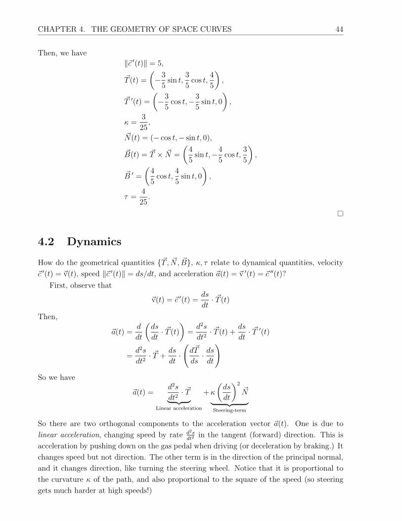
CHAPTER 4. THE GEOMETRY OF SPACE CURVES 44
Then, we have
‖~c ′(t)‖ = 5,
~T (t) =
(−3
5sin t,
3
5cos t,
4
5
),
~T ′(t) =
(−3
5cos t,−3
5sin t, 0
),
κ =3
25,
~N(t) = (− cos t,− sin t, 0),
~B(t) = ~T × ~N =
(4
5sin t,−4
5cos t,
3
5
),
~B ′ =
(4
5cos t,
4
5sin t, 0
),
τ =4
25.
4.2 Dynamics
How do the geometrical quantities {~T , ~N, ~B}, κ, τ relate to dynamical quantities, velocity
~c ′(t) = ~v(t), speed ‖~c ′(t)‖ = ds/dt, and acceleration ~a(t) = ~v ′(t) = ~c ′′(t)?
First, observe that
~v(t) = ~c ′(t) =ds
dt· ~T (t)
Then,
~a(t) =d
dt
(ds
dt· ~T (t)
)=d2s
dt2· ~T (t) +
ds
dt· ~T ′(t)
=d2s
dt2· ~T +
ds
dt·(d~T
ds· dsdt
)So we have
~a(t) =d2s
dt2· ~T︸ ︷︷ ︸
Linear acceleration
+κ
(ds
dt
)2
~N︸ ︷︷ ︸Steering-term
So there are two orthogonal components to the acceleration vector ~a(t). One is due to
linear acceleration, changing speed by rate d2sdt2
in the tangent (forward) direction. This is
acceleration by pushing down on the gas pedal when driving (or deceleration by braking.) It
changes speed but not direction. The other term is in the direction of the principal normal,
and it changes direction, like turning the steering wheel. Notice that it is proportional to
the curvature κ of the path, and also proportional to the square of the speed (so steering
gets much harder at high speeds!)
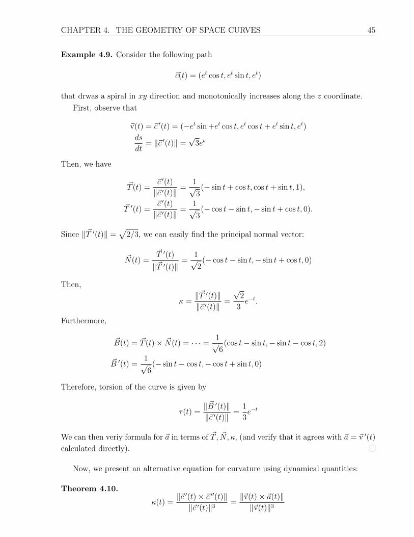
CHAPTER 4. THE GEOMETRY OF SPACE CURVES 45
Example 4.9. Consider the following path
~c(t) = (et cos t, et sin t, et)
that drwas a spiral in xy direction and monotonically increases along the z coordinate.
First, observe that
~v(t) = ~c ′(t) = (−et sin +et cos t, et cos t+ et sin t, et)
ds
dt= ‖~c ′(t)‖ =
√3et
Then, we have
~T (t) =~c ′(t)
‖~c ′(t)‖ =1√3
(− sin t+ cos t, cos t+ sin t, 1),
~T ′(t) =~c ′(t)
‖~c ′(t)‖ =1√3
(− cos t− sin t,− sin t+ cos t, 0).
Since ‖~T ′(t)‖ =√
2/3, we can easily find the principal normal vector:
~N(t) =~T ′(t)
‖~T ′(t)‖=
1√2
(− cos t− sin t,− sin t+ cos t, 0)
Then,
κ =‖~T ′(t)‖‖~c ′(t)‖ =
√2
3e−t.
Furthermore,
~B(t) = ~T (t)× ~N(t) = · · · = 1√6
(cos t− sin t,− sin t− cos t, 2)
~B ′(t) =1√6
(− sin t− cos t,− cos t+ sin t, 0)
Therefore, torsion of the curve is given by
τ(t) =‖ ~B ′(t)‖‖~c ′(t)‖ =
1
3e−t
We can then veriy formula for ~a in terms of ~T , ~N, κ, (and verify that it agrees with ~a = ~v ′(t)
calculated directly).
Now, we present an alternative equation for curvature using dynamical quantities:
Theorem 4.10.
κ(t) =‖~c ′(t)× ~c ′′(t)‖‖~c ′(t)‖3 =
‖~v(t)× ~a(t)‖‖~v(t)‖3

CHAPTER 4. THE GEOMETRY OF SPACE CURVES 46
Proof. To verify it, we use the decomposition of ~a:
~v × ~a = ~v ×(d2s
dt2· ~T + κ
(ds
dt
)2
~N
)
=d2s
dt2
(~v × ~T
)+ κ
(ds
dt
)2 (~v × ~N
)= κ
(ds
dt
)3 (~T × ~N
)= κ
(ds
dt
)3
~B
Then, κ(ds/dt)3‖ ~B‖ = ‖~v × ~a‖. Since ~B is a unit vector, we get the desired identity by
taking the norm on each side of the equation.
4.3 Practice problems
Practice problems will be given from Stewart [Stew].

Chapter 5
Implicit functions
5.1 The Implicit Function Theorem I
Often, we have an implicit relationship between variables,
F (x1, x2, . . . , xn) = 0,
rather than an explicit function relation, such as
xn = f(x1, x2, . . . , xn−1).
Example 5.1. Look at a familiar example in R2 (See Figure 5.1), the unit circle,
x2 + y2 = 1.
This fails vertical line test (y 6= f(x)) as well as horizontal line test (x 6= g(y)); globally,
this relation does not define a function. Locally, we can write this as a function, i.e. by
restricting attention to small pieces of the curve.
First, define
F (x, y) = x2 + y2 − 1
If y0 > 0, x20 + y20 = 1, i.e. F (x0, y0) = 0, and we look at a window (or neighborhood) around
(x0, y0), which lies entirely in the upper half plane, we can solve for y = f(x),
y =√
1− x2︸ ︷︷ ︸f(x)
We could calculate y′ = f ′(x) from the explicit formula but we can also get it via implicit
differentiation:d
dx(F (x, f(x))) =
∂F
∂x· dxdx
+∂F
∂y· f ′(x)
= 2x+ 2yf ′(x),
so f ′(x) = −x/y.
47

CHAPTER 5. IMPLICIT FUNCTIONS 48
x
y
A
B
F (x, y) = x2 + y2 − 1
Figure 5.1. Near the neighborhood around point A, vertical line test fails as single xvalue corresponds to two y values. On the other hand, neighborhood around point B canbe solved as y =
√1− x2.
For a general F (x, y) = 0, we can solve for f ′(x) if
∂F
∂y(x0, y0) 6= 0,
where y is the variable we want to solve for. This gives the limitation on which we can solve
for y = f(x) locally. For the circle example, we had
∂F
∂y= 2y.
When y = 0, the vertical line test fails in every neighborhood of (x0, y0) = (±1, 0), which is
exactly when the partial derivative with respect to y vanishes.
In general, suppose we have a C1 function,
F : Rn+1 → R,
and consider all functions of F (~x, y) = 0. In order to write y = g(~x) – i.e. we can solve for
y as a differentiable function of ~x – we do the same implicit differentiation, with the chain
rule,∂
∂xi(F (x1, x2. . . . .xn, f(~x))) =
∂F
∂xi+∂F
∂y
∂f
∂xi
for each i = 1, 2, . . . , n. We can then solve for each
∂f
∂xi=− ∂F
∂xi∂F
∂y
,
provided ∂F/∂y 6= 0. This is a sufficient condition to solve for y = f(~x).

CHAPTER 5. IMPLICIT FUNCTIONS 49
Theorem 5.2 (Implicit Function Theorem I). Assume F : Rn+1 → R is C1 in a neighbor-
hood of (~x0, y0) with F (~x0, y0) = 0. If ∂F∂y
(~x0, y0) 6= 0, then there exists neighborhood U of ~x0
and V of y0 and a C1 function
f : U ⊂ Rn → V ⊂ R,
for which F (~x, f(~x)) = 0 for all ~x ∈ U . In addition,
Df(~x) =− 1
∂F
∂y(~x, y)
D~xF (~x, y),
where
D~xF (~x, y) =[∂F∂x1
∂F∂x2
· · · ∂F∂xn
].
Example 5.3. Consider the following function:
xy + y2z + z3 = 1.
For which part on this surface can we write z = f(x, y), i.e.
F : R3 → R, F (x, y, z) = xy + y2z + z3 − 1
is C1?
We want to solve for z, so we look at
∂F
∂z= y2 + 3z2
We observe that ∂F/∂z = 0 iff y = 0 and z = 0. However, y = 0 and z = 0 is not defined
on this surface. At all points on this surface, ∂F/∂z 6= 0. So at every (x0, y0, z0) with
F (x0, y0, z0) = 0, we can solve for z = f(x, y) locally near (x0, y0).
We can then use the implicit differentiation formula in the theorem to calculate Df(x, y):
D(x,y)F =[y (x+ 2yz)
],
so we get
Df(x, y) =−D(x,y)F
∂F/∂z=
[− y
y2 + 3z2−x+ 2yz
y23z2
]or
∇f(x, y) =
(− y
y2 + 3z2,− x+ 2yz
y2 + 3z2
).
Example 5.4. Consider the following equation:
x4 + xz2 + z4 = 1.
Show that we can solve for z = g(x) near (x1, z1) = (−1, 1) but not near (x2, z2) = (1, 0).

CHAPTER 5. IMPLICIT FUNCTIONS 50
Proof. First, let
F (x, z) = x4 + xz2 + z4 − 1.
Clearly, F : R2 → R is C1 for all (x, z) ∈ R2. Observe that
∂F
∂z= 2xz + 4z3,
and so ∂F (−1, 1)/∂z 6= 0.
By the Implicit Function Theorem, we can solve for z = g(x) locally near (x1, z1) =
(−1, 1). In addition, we can get an explicit formula for its derivative:
Dg(x) = g′(x) = −∂F (x, z)/∂x
∂F/∂z= − 4x3 + z2
2xz + 4z3
Finally, since ∂F (1, 0)/∂z = 0, the Implicit Function Theorem does not apply near
(1, 0). This does not mean that you cannot solve for z as a function of (x, z) locally
near (1, 0) (see Example 5.5 below.) Nevertheless, in this example it is the case that we
can’t solve for z = g(x) locally near (1, 0). Notice that F is even symmetric in z, that is
F (x,−z) = F (x, z) for all (x, z). So for every point (x, z) which solves F (x, z) = 0, it’s also
true that F (x,−z) = 0. This means that for every x there are two values ±z lying on the
curve described by F (x, z) = 0. (So we can not solve x = g(z) globally, as the vertical line
rule fails unless z = 0.) When z 6= 0 this is all right, since the points (x, z) and (x,−z)
are far apart, so we can solve locally, but in any neighborhood of (x, z) = (1, 0) there are
always two points (x,±z) and the curve is not a function locally near (1, 0).
Example 5.5. As mentioned above, it’s possible that the hypotheses of the Implicit Func-
tion Theorem are not satisfied, but it is still possible to solve for z = g(x) with C1 func-
tion g anyway. This may seem silly, but it’s a legitimate example: take F : R2 → Ras F (x, z) = (z − x2)2. Then F is C1, and F (x, z) = 0 is equivalent to (z − x2) = 0,
which is equivalent to z = x2, and the curve is globally described by the C1 graph of
g(x) = x2. The Implicit Function Theorem does not apply at any (x, z) on the curve, since∂F∂z
= 2(z − x2) = 0 at every point.
Example 5.6. Intermediate situations are also possible when the hypotheses of the Implicit
Function Theorem fail to hold. Consider the following equation:
x− z3 = 0
Clearly, F (x, z) = x− z3 is C1 for all (x, z) ∈ R2. Note that
∂F
∂z= −3z2.
Clearly, ∂F/∂z = 0 at (x, z) = (0, 0). However, we can write z = x1/3 globally. So an
explicit representation of z as a function of x exists, z = g(x) = x1/3. On the other hand,
g(x) isn’t differentiable at (x0, z0) = (0, 0), so the vanishing of the partial derivative ∂F∂z
is
making itself felt in a more subtle way.

CHAPTER 5. IMPLICIT FUNCTIONS 51
5.2 The Implicit Function Theorem II
We also have a version of the Implicit Function Theorem which applies to under-determined
systems of (nonlinear) equations.
Example 5.7. Suppose we have a system of equations with more unknowns:{u2 − v2 − x3 = 0
2uv − y5 = 0
Can we solve for (u, v) as functions of (x, y)?
First, consider a C1 function, F : R4 → R2, that is defined as follows:{F1(x, y, u, v) = u2 − v2 − x2 = 0
F2(x, y, u, v) = 2uv − y5 = 0
Following what we did before, we can assume (u, v) = g(x, y) and see when we can
calculate Dg. Note that
0 =∂
∂xF1(x, y, u(x, y), v(x, y)) =
∂F1
∂x+∂F1
∂u
∂u
∂x+∂F1
∂v
∂v
∂x
0 =∂
∂xF2(x, y, u(x, y), v(x, y)) =
∂F2
∂x+∂F2
∂u
∂u
∂x+∂F2
∂v
∂v
∂x
Then, we can solve for ∂u/∂x and ∂v/∂x. Rearranging,∂F1
∂u
∂F1
∂v∂F2
∂u
∂F2
∂v
∂u∂x∂v
∂x
=
−∂F1
∂x
−∂F2
∂x
This can be solved if D(u,v)F is invertible, i.e. det
[D(u,v)F
]6= 0.
Similarly, we can also solve for ∂u/∂y and ∂v/∂y. As a result, we get a different linear
system to solve but with the same matrix[D(u,v)F
]. The second version of the Implicit
Function Theorem says that this is the correct condition to solve for g(x) in this setting.
Let’s see how this works in general. The notation is a bit complicated, but the basic
idea is the same as in the example. Given the following system of functions,
F1(x1, . . . , xn, u1, . . . um) = 0
F2(x1, . . . , xn, u1, . . . um) = 0
...
Fm(x1, . . . , xn, u1, . . . um) = 0
we want to solve for ~u = (u1, . . . , um) ∈ Rm as a function, ~u = g(~x), of ~x = (x1, . . . , xn) ∈ Rn.
Via implicit differentiation, for the case of n = m = 2, we arrived at an appropriate condition
where this is possible.

CHAPTER 5. IMPLICIT FUNCTIONS 52
Theorem 5.8 (Implicit Function Theorem II - General Form). Let
F : Rn+m → Rm
be a C1 function in a neighborhood of (~x0, ~u0) ∈ Rn+m, with F (~x0, ~u0) = ~0. If, in addition,
D~uF (~x0, ~u0) is invertible, then there exists neighborhoods V of ~x0 and U of ~u0, for which
solutions of F (~x, ~u) = ~0 lie on a C1 graph, ~u = g(~x),
g : V ⊂ Rn → U ∈ Rm
Example 5.9. Consider the following set of equations:{2xu2 + yv4 = 3
xy(u2 − v2) = 0
Can we solve for (u, v) = g(x, y) near (x0, y0, y0, v0) = (1, 1,−1,−1)?
Let
F =
[F1
F2
], ~x = (x, y), ~u = (u, v),
where F is defined asF1(~x, ~u) = 2xu2 + yv4 − 3 = 0
F2(~x, ~u) = xy(u2 − v2) = 0)
}(5.1)
Then, we get the following Jacobian
D~uF =∂(F1, F2)
∂(u, v)
=
∂F1
∂u
∂F1
∂v∂F2
∂u
∂F2
∂v
=
[4xu 4yv3
2uxy −2vxy
]Substituting the given values, we have
D~uF (1, 1,−1,−1) =
[−4 −4−2 2
]Since detD~uF = −16 6= 0, the Implicit Function Theorem does apply, and we can solve for
~u = (u, v) = g(~x) = g(x, y) near (x0, y0, u0, v0) = (1, 1,−1,−1).
In general, we can’t get an explicit formula for g, but we can get a formula for Dg(x, y),
i.e. its partial derivatives, using implicit differentiation. For the above example, we may cal-
culate ∂u∂x, ∂v∂x
by implicitly differentiating the equations (5.1) with respect to x, remembering
that u, v are functions of (x, y):
0 =∂F1
∂x=
∂
∂x
[2xu2 + yv4 − 3
]= 2u2 + 4xuux + 4yv3 vx
0 =∂F1
∂x=
∂
∂x
[xy(u2 − v2)
]= y(u2 − v2) + xy(2uux − 2v vx).
CHAPTER 5. IMPLICIT FUNCTIONS 53
At (x, y, u, v) = (1, 1,−1,−1) we obtain the system of equations,
−4ux − 4vx = −2
−2ux + 2vx = 0.
Notice that the coefficient matrix is exactly D~uF (1, 1,−1,−1). This is not an accident!
Using Cramer’s Rule1 the system may be easily solved using determinants, and we have
ux(1, 1) = vx(1, 1) = 14. To find uy(1, 1), vy(1, 1), do the same thing but take the implicit
derivative with respect to y.
5.3 Inverse Function Theorem
In general, suppose we have a C1 function, f : Rn → Rn, where ~x = f(~u). Is it possible to
solve for ~u = g(~x)?
In single-variable calculus, a function f : R→ R is one-to-one on an interval [a, b] if and
only if f is strictly monotone on [a, b]. For these functions, f has an inverse g = f−1,
g(f(x)) = x, ∀x ∈ [a, b]
If f is differentiable on [a, b], and f ′(x) > 0 on [a, b] (or f ′(x) < 0 on [a, b]), then the
inverse g(x) is also differentiable, and
g′(f(x)) =1
f ′(x), ∀x ∈ [a, b]
If, for example, f ′(x) > 0 for all x ∈ R, then it’s globally invertible, i.e. g(f(x)) = x for all
x ∈ R. How do we apply this for f : Rn → Rn with n ≥ 2? There’s no such thing as a
monotone function of several variables!
Let’s look at a simple example for guidance.
Example 5.10. Consider the following set of equations:{x = u2 − v2y = 2uv
1 Cramer’s Rule. Given a system of linear equations that is represented by 2× 2 matrices,{ax+ by = s
cx+ dy = t,
solution of the system is given by
x =
det
(s bt d
)det
(a bc d
) , y =
det
(a sc t
)det
(a bc d
)

CHAPTER 5. IMPLICIT FUNCTIONS 54
Note that this example fits the form of the Implicit Function Theorem, but it’s a special
case. We want to invert this relation, i.e. given, ~x = f(~u), we want to solve for ~u = g(~x).
To get a nice theorem for this special case, we can use the framework of the Implicit
Function Theorem: {F1(~x, ~u) = f1(~u)− x = 0
F2(~x, ~u) = f2(~u)− y = 0
Since
D~uF (~x, ~u) = Df(~u),
we can do this locally near a point (~x0, ~u0) provided that
det (Df(~u)) 6= 0
This is a very satisfying result, because it’s a direct extension of the linear algebra case.
If we had a linear change of variables, ~x = M~u with a constant matrix M , we can solve
~u = M−1~x provided detM 6= 0. So while it makes no sense to calculate the determinant of
a nonlinear function, it turns out that the nonlinear function is invertible (at least locally)
when its derivative matrix is invertible!
Theorem 5.11 (Inverse Function Theorem). Suppose f : Rn → Rn which is C1 in a
neighborhood of ~u0, with f(~u0) = ~x0. If det (Df(~u0)) 6= 0, then there exist neighborhoods Uof ~u0 and V of ~x0 and a C1 function g : V → U , with
~x = f(~u)with ~u∈U
⇐⇒ ~u = g(~x)with ~x∈V
,
i.e. near ~x0 and ~u0, g is the inverse of f .
Moreover,
Dg(~x) = [Df(~u)]−1 . (5.2)
The formula for the derivative matrix of the inverse function follows directly from the
Chain Rule: since ~x = f(~u) = f(g(~x)), ignore the middle equality and differentiate with
respect to ~x. Since the function h(~x) = ~x = I~x, with I the identity matrix, Dh(~x) = I. So
I = Dh(~x) = D(f ◦ g(~x)) = Df(~u)Dg(~x).
Since we are assuming in the theorem that det(Df(~u)) 6= 0, the matrix is invertible, and
the above formula (5.2) is verified.
Example 5.12. Apply the Inverse Function Theorem to the function that was defined in
the previous example: {x = u2 − v2y = 2uv

CHAPTER 5. IMPLICIT FUNCTIONS 55
Observe that
det (Df(u, v)) = det
[2u −2v2v 2u
]= 4u2 + 4v2 6= 0
as long as (u0, v0) 6= (0, 0). So we can invert the variables and solve for (u, v) = g(x, y),
locally near any (u0, v0) 6= (0, 0).
Notice thatf1(−u,−v) = x = f1(u, v)
f2(−u,−v) = y = f2(u, v)
So in any neighborhood of (0, 0) there are 2 values of (u, v) corresponding to each (x, y).
Therefore, f is not invertible near (u, v) = (0, 0).
Example 5.13. Consider the following equations:{x = ey cos v
y = eu sin v
For which (u, v, x, y) can we solve for u, v as functions of x, y?
Let
f(u, v) =
[eu cos veu sin v
].
Then, we have
Df(u, v) =
[eu cos v −eu sin veu sin v eu cos v
]Then, we can compute det(Df(u, v)), (or det
(∂(x,y)∂(u,v)
)):
det(Df(u, v)) = e2u.
Clearly, det(Df(u, v)) > 0 for all u, v. By the Inverse Function Theorem, we can invert and
solve for (u, v) = g(x, y), near any (u0, v0).
We can invert locally near any point; can we find a global inverse, i.e. a g for which
(u, v) = g(x, y) for every (u, v) ∈ R2? If so, then f would have to be a one-to-one function.
However,
f(u, v + 2πk) = f(u, v)
for all k ∈ Z. Therefore, f can’t be globally inverted.
Example 5.14. Consider the following equations:{x = f1(u, v) = u3 − 3uv2
y = f2(u, v) = −v3 + 3u2v
Since they’re polynomials, f : R2 → R2 is C1. Then, we have
∂(x, y)
∂(u, v)=
[3u2 − 3v2 −6uv
6uv −3v2 + 3u2
]det
(∂(x, y)
∂(u, v)
)= (3u2 − 3v2)2 + (6uv)2

CHAPTER 5. IMPLICIT FUNCTIONS 56
Clearly, det (∂(x, y)/∂(u, v)) = 0 iff u = v = 0. So, Inverse Function Theorem holds for all
(u0, v0) 6= (0, 0), and we can solve for (x, y) = g(u, v) around any (u0, v0) 6= (0, 0).
5.4 Practice problems
1. [MT, p. 210] Show that the equation x+y−z+cos(xyz) = 1 can be solved for z = g(x, y)
near the origin. Find ∂g∂x
and ∂g∂y
at (0,0).
2. [MT, p. 210] Show that xy + z + 3xz5 = 4 is solvable for z as a function of (x, y) near
(1, 0, 1). Compute ∂z/∂x and ∂z/∂y at (1, 0).
3. [MT, p. 210]
(a). Check directly where we can solve the equation
F (x, y) = y2 + y + 3x+ 1 = 0
for y in terms of x.
(b). Check that your answer in part (a) agrees with the answer you expect from the
implicit function theorem. Compute dy/dx.
4. [MT, p. 210] Repeat problem 3 with
F (x, y) = xy2 − 2y + x2 + 2 = 0.
5. [MT, p. 210] Let F (x, y) = 0 define a curve in the xy plane through the point (x0, y0),
where F is C1. Assume that (∂F/∂y)(x0, y0) 6= 0. Show that this curve can be locally
represented by the graph of a function y = g(x). Show that (i) the line orthogonal to
∇F (x0, y0) agrees with (ii) the tangent line to the graph of y = g(x).
6. [MT, p. 210] Show that x3z2 − z3yx = 0 is solvable for z as a function of (x, y) near
(1, 1, 1), but not near the origin. Compute ∂z/∂x and ∂z/∂y at (1, 1).
7. [MT, p. 210] Investigate whether or not the system
u(x, y, z) = x+ xyz
v(x, y, z) = y + xy
w(x, y, z) = z + 2x+ 3z2
can be solved for x, y, z in terms of u, v, w near (x, y, z) = (0, 0, 0).
8. [MT, p. 210] Let (x0, y0, z0) be a point of the locus defined by x2 + xy − a = 0,
z2 + x2 − y2 − b = 0, where a and b are continuous.

CHAPTER 5. IMPLICIT FUNCTIONS 57
(a) Under what conditions may the part of the locus near (x0, y0, z0) be represented in
the form x = f(z), y = g(z)?
(b) Compute f ′(z) and g′(z).
9. [MT, p. 211] Let F (x, y) = x3−y2 and let C denote the level curve given by F (x, y) = 0.
(a) Without using the implicit function theorem, show that we can describe C as the
graph of x as a function of y near any point.
(b) Show that Fx(0, 0) = 0. Does this contradict the implicit function theorem?
10. [MT, p. 211] Consider the system of equations
x5v2 + 2y3u = 3
3yu− xuv3 = 2.
Show that near the point (x, y, u, v) = (1, 1, 1, 1), this system defines u and v implicitly
as functions of x and y. For such local functions u and v, define the local function f by
f(x, y) = (u(x, y), v(x, y)). Find Df(1, 1).
11. [MT, p. 211] Consider the equations
x2 − y2 − u3 + v2 + 4 = 0
2xy + y2 − 2u2 + 3v4 + 8 = 0.
(a) Show that these equations determine functions u(x, y) and v(x, y) near the point
(x, y, u, v) = (2,−1, 2, 1).
(b) Compute ∂u∂x
at (x, y) = (2,−1).

CHAPTER 5. IMPLICIT FUNCTIONS 58

Chapter 6
Taylor’s Theorem and critical points
6.1 Taylor’s Theorem in one dimension
Consider a one-dimensional function:
g : R→ R,
which is Ck+1, i.e. it is (k + 1) times continuously differentiable; i.e., each derivative,
djg
dxj(t), j = 1, 2, . . . , k + 1, (of order up to and including the (k + 1)st),
exists and is a continuous function (in some interval). Then, we can approximate g(x)
locally near t = a by a polynomial of degree k, Taylor’s polynomial, Pk(t):
Pk(t) = g(a) + g′(a)(t− a) +1
2!g′′(a)(t− a)2 + · · ·+ 1
k!
dkg
dtk(a)(t− a)k
The Taylor coefficients are chosen to match g(t) up to the kth derivative at t = a,
djPkdtj
(a) =djg
dtj(a), j = 0, 1, 2, . . . , k.
To review this material, look back to section 11.11 in Stewart [Stew]. There, the emphasis
was on the Taylor Series, and questions of its convergence, but here we are interested in trun-
cating the series for the purpose of approximation. And in any question of approximation
the error made (the remainder term) is of the highest importance.
For example, P1(t) = g(a) + g′(a)(t − a) is the tangent line. Since we know that g is
differentiable,
limt→a
|g(t)− P1(t)||t− a| = 0 or g(t) = P1(t) + o(|t− a|)
Theorem 6.1 (Taylor’s Theorem, 1D version). Assume g : R → R is Ck+1 in a neighbor-
hood of t = a. Then, for each t, there exists c between a and t for which
g(t) = Pk(t) +Rk(a, t),
with remainder Rk(a, t) = dk+1gdtk+1 (c)(t− a)k+1.
59

CHAPTER 6. TAYLOR’S THEOREM AND CRITICAL POINTS 60
Since we assumed that dk+1gdtk+1 is continuous, the remainder term is very small when t→ a,
limt→a
Rk(a, t)
|t− a|k = 0,
i.e. Rk(a, t) = o(|t− a|k
). So Rk(a, t) is small compared with each of the terms appearing
in Pk(t).
Remark. Locally, g(t) is well approximated by its Taylor polynomial, but only near x = a.
Example 6.2. For g(t) = cos t at a = 0, we look at the 3rd order Taylor polynomial:
g(0) = cos 0 = 1, g′(0) = − sin 0 = 0, g′′(0) = − cos(0) = −1, g′′′(0) = sin 0 = 0.
Therefore, Taylor’s Theorem implies that for t near 0, and
g(t) = cos t = 1− 0t− 1
2t2 + 0t3︸ ︷︷ ︸
P3(t)
+R3(0, t) = 1− 1
2t2 + o(t3).
This tells us that cos t is approximately quadratic near a = 0, with an error which is very
small compared to t3 (it is of the order of t4.) This is local information, as the graph of
cos t doesn’t look in the least like an inverted parabola when t is large, since the cosine
oscillates periodically between ±1 while the parabola diverges to −∞ for t → ±∞. (See
Figure 6.1.)
y = cosx
y = 1− 12x2
Figure 6.1. Third degree Taylor expansion of cos x tells us that the curve is locallyquadratic near x = 0.
6.2 Taylor’s Theorem in higher dimensions
To obtain a version of Taylor’s Theorem in several variables we apply the one-dimensional
version in a careful way, by restricting our attention to each line, ~x = ~a + t~u, through ~a in
direction ~u.

CHAPTER 6. TAYLOR’S THEOREM AND CRITICAL POINTS 61
Assume f ∈ C3 near ~a ∈ Rn. Let’s sample f(~x) along a line running through x0. Take
a unit vector ~u, ‖~u‖ = 1, and the line,
~l(t) = ~a+ t~u,
that goes through ~a at t = 0 in the direction of ~u. Then, we let
g(t) = f(~l(t)) = f(~a+ t~u),
so g : R → R. By the chain rule, if f is C3 near ~a, then g is C3 near t = 0, and so we
may apply Taylor’s Theorem to g to approximate its values near t = 0. In doing so, we will
generate a Taylor expansion for f(~x) with x = ~a+ t~u.
We calculate the terms in the Taylor polynomial for g, which has the form,
g(t) = g(0) + g′(0)(t− 0) +1
2g′′(0)(t− 0)2 +R2, with R2 = o(t2).
We begin with:g(0) = f(~a),
g′(t) = Df(~a+ t~u) ·~l ′(t) = Df(~a+ t~u)~u.
So g′(0) = Df(~a)~u = ∇f(~a) · ~u. Using the definition ~x = ~l(t) = ~a+ t~u, we have t~u = ~x−~a,
and so the first derivative term may be rewritten as
g′(0)(t− 0) = Df(~a)[~x− ~a].
Finding the second derivative is a little tricky. We write the first derivative out in its
coordinates,
g′(t) =n∑i=1
∂f
∂xi(~a+ t~u)ui.
Then we use the Chain Rule in the form you learned last year to calculate
g′′(t) =n∑i=1
d
dt
(∂f
∂xi(~a+ t~u)
)ui =
n∑i=1
n∑j=1
∂2f
∂xi∂xj(~a+ t~u)ujui
Therefore,
g′′(0) =n∑i=1
n∑j=1
∂2f
∂xi∂xj(~a)uj ui,
which is a quadratic form with matrix
H(~x) =
[∂2f
∂xi∂xj(~a)
]i,j=1,...,n
,
the Hessian matrix of f at ~a. We will also write H(~x) = D2f(~x), as it is the matrix of all
second partial derivatives of f . For f a C2 function, fxixj = fxjxi , so H(~a) is a symmetric
matrix. Again using t~u = ~x− ~a, we may then write
g′′(0)(t− 0)2 = t~u ·H(~a)t~u = [~x− ~x0] ·H(~a)[~x− ~a].
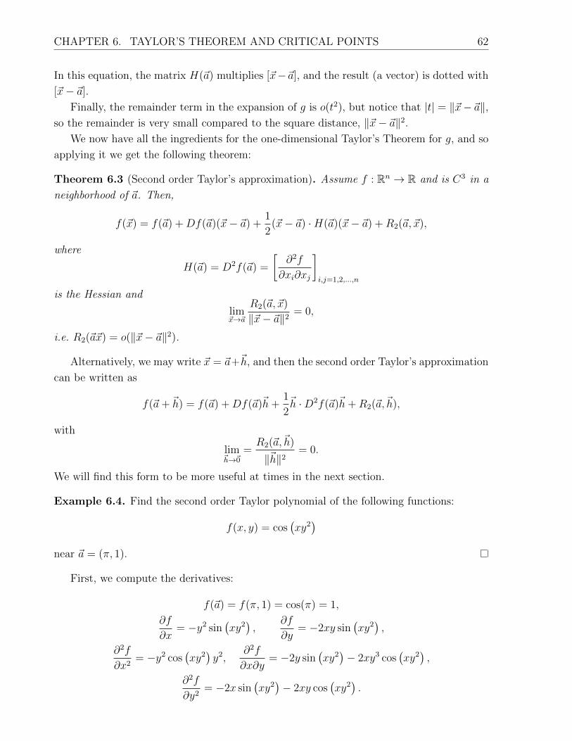
CHAPTER 6. TAYLOR’S THEOREM AND CRITICAL POINTS 62
In this equation, the matrix H(~a) multiplies [~x−~a], and the result (a vector) is dotted with
[~x− ~a].
Finally, the remainder term in the expansion of g is o(t2), but notice that |t| = ‖~x−~a‖,so the remainder is very small compared to the square distance, ‖~x− ~a‖2.
We now have all the ingredients for the one-dimensional Taylor’s Theorem for g, and so
applying it we get the following theorem:
Theorem 6.3 (Second order Taylor’s approximation). Assume f : Rn → R and is C3 in a
neighborhood of ~a. Then,
f(~x) = f(~a) +Df(~a)(~x− ~a) +1
2(~x− ~a) ·H(~a)(~x− ~a) +R2(~a, ~x),
where
H(~a) = D2f(~a) =
[∂2f
∂xi∂xj
]i,j=1,2,...,n
is the Hessian and
lim~x→~a
R2(~a, ~x)
‖~x− ~a‖2 = 0,
i.e. R2(~a~x) = o(‖~x− ~a‖2).
Alternatively, we may write ~x = ~a+~h, and then the second order Taylor’s approximation
can be written as
f(~a+ ~h) = f(~a) +Df(~a)~h+1
2~h ·D2f(~a)~h+R2(~a,~h),
with
lim~h→~0
=R2(~a,~h)
‖~h‖2= 0.
We will find this form to be more useful at times in the next section.
Example 6.4. Find the second order Taylor polynomial of the following functions:
f(x, y) = cos(xy2)
near ~a = (π, 1).
First, we compute the derivatives:
f(~a) = f(π, 1) = cos(π) = 1,
∂f
∂x= −y2 sin
(xy2),
∂f
∂y= −2xy sin
(xy2),
∂2f
∂x2= −y2 cos
(xy2)y2,
∂2f
∂x∂y= −2y sin
(xy2)− 2xy3 cos
(xy2),
∂2f
∂y2= −2x sin
(xy2)− 2xy cos
(xy2).

CHAPTER 6. TAYLOR’S THEOREM AND CRITICAL POINTS 63
Then, at ~a = (π, 1), we find that
Df(~a) =[0 0
]D2f(~a) =
[1 2π
2π 4π2
]So, we have
f(~a+ ~h) = −1 +1
2~h ·[
1 2π2π 4π2
]~h+R2
f(π + h1, 1 + h2) = −1 +1
2
[h1h2
]·[h1 + 2πh2
2πh1 + 4π2h2
]= −1 +
1
2
(h21 + 4πh1h2 + 4π2h22
)+ o(‖~h2‖)
In terms of a point ~x (near ~a), we can write ~x = ~a+ ~h, so ~h = ~x− ~a, and then
cos(xy2)
= −1 +1
2
((x− a1)2 + 4π(x− a1)(y − a2) + 4π2(y − a2)2
)+R2,
and R2 = o(‖~x − ~a‖2. The advantage of the f(~a + ~h) form is that it is easier to guess the
behaviour of f(~x) near ~x = ~a. This is what we will do in the next section, to classify critical
points as maxima and minima!
6.3 Local minima/maxima
This is exactly the same definition as in Stewart [Stew], only generalized to Rn. (So if you
were paying attention to the definitions last year, this is old news!)
Definition 6.5. We say ~a is a local minimum for f if there exists an open disk Dr(~a) for
which
f(~a) ≤ f(~x)
for all ~x ∈ Dr(~a). ~a is a strict local minimum if
f(~a) < f(~x)
for all ~x 6= ~a, ~x ∈ Dr(~a).
Definition 6.6. We say ~a is a local maximum for f if ∃r > 0 with f(~a) ≥ f(~x), ∀~x ∈ Dr(~a).
~a is a strict local max if f(~a) > f(~x), ∀~x ∈ Dr(~a) \ {~a}.
Example 6.7. As you have seen from your previous multivariable course, f(x, y) = x2 + y2
has a local minimum (in fact, the global minimum) at (x, y) = (0, 0), and g(x, y) = −x2−y2has a local maximum (in fact, the global maximum) at (x, y) = (0, 0). Verifying this directly
is not hard, since a sum of squares is always non-negative, and so
f(0, 0) = 0 ≤ x2 + y2 = f(x, y), for all (x, y) ∈ R2.
We leave the verification for g(x, y) as an exercise.
CHAPTER 6. TAYLOR’S THEOREM AND CRITICAL POINTS 64
Note that if f is differentiable, we have a necessary condition for local maxima and
minima: they can only occur at a critical point of f :
Theorem 6.8. If f has a local maxima or minima at ~a and is differentiable at ~a, then
Df(~a) = ~0.
Proof. Again, we start by restricting to line through ~a:
g(t) = f(~a+ t~u),
where ~u is a unit vector. If f has a local minima at ~a, then
g(0) = f(~a) ≤ f(~a+ t~u) = g(t),
for all t with |t| < r. So g(t) has a local minima at t = 0. By a calculus theorem, g′(0) = 0.
But,
0 = g′(0) = Df(~a)~u,
for all ~u. Then, by taking ~u = ~e1, ~e2 . . . , ~en, we get
∂f
∂xj(~a) = 0,
for each j = 1, 2, 3, . . . , n. Therfore, Df(~a) = 0.
Definition 6.9. An ~a for which Df(~a) = 0 is called a critical point.
Example 6.10. In Example 6.4 , ~a = (π, 1) was a critical point.
Recall that not all critical points must be local maxima or minima, even in one dimension.
But in higher dimensions the possible variety of critical point behavior is much larger.
Now, we want to combine Taylor’s Theorem and linear algebra to classify critical points
as local minima, maxima, or other. Taylor’s theorem states that for ~x = ~a + ~h, if ‖~h‖ is
small,
f(~x) = f(~a+ ~h) = f(~a) +Df(~a)~h︸ ︷︷ ︸0
+1
2~h ·D2f(~a)~h︸ ︷︷ ︸quadratic form
+R2(~a,~h)︸ ︷︷ ︸o(‖~h‖2)
(6.1)
So we expect the behaviour of f(~x) near ~a to be determined by the quadratic term.
Recall that the Hessian matrix, M = D2f(~a), is a symmetric matrix. This allows us to
apply the following theorem:
Theorem 6.11 (The Spectral Theorem). Assume M is a symmetric (n×n) matrix. Then,
• All eigenvalues of M are real, λi ∈ R ∀i = 1, 2, . . . , n.
• There is an orthonormal basis {~u1, ~u2, . . . , ~un} of Rn composed ot eigenvalues of M ,
M~ui = λi~ui, ‖~ui‖ = 1, ~ui · ~uj = 0 for i 6= j

CHAPTER 6. TAYLOR’S THEOREM AND CRITICAL POINTS 65
• In the basis of eigenvalues, M is a diagonal matrix. In other words, if we let U be the
matrix whose columns are the ~ui; then
MU = UΛ,
where Λ = diag(λ1, λ2, . . . , λn).
Remark. Note that since the eigenvalues are real, they can be ordered, smallest to largest:
λ1 ≤ λ2 ≤ · · · ≤ λn.
However, they may not be necessarily distinct. (For example, the identity matrix I has each
λj = 1.)
Written in the orthonormal basis of eigenvalues, the quadratic form, ~h · M~h, has an
easy expression. First, since the ~ui form a basis, any vector may be expressed as a linear
combination,
~h =n∑i=1
ci~ui,
with coefficients ci ∈ R, i = 1, 2, . . . , n. Notice that
~h · uj =n∑i=1
ci~ui · ~uj = cj, (6.2)
since ~ui · ~uj = 0 if i 6= j and ~ui · ~uj = 1 if i = j. In particular, we can evaluate the norm of~h in terms of the coefficients ci,
‖~h‖2 = ~h · ~h = ~h ·(
n∑j=1
cj~uj
)
=n∑j=1
cj ~h · ~ui
=n∑j=1
c2j , (6.3)
using (6.2).
To evaluate the quadratic form we make a similar calculation, using the orthogonality
of the normalized eigenvectors:
~h ·M~h = ~h ·n∑i=1
ciM~ui
= ~h ·n∑i=1
λici~ui
=n∑i=1
λici(~h · ~ui︸ ︷︷ ︸ci
)
=n∑i=1
λic2i (6.4)

CHAPTER 6. TAYLOR’S THEOREM AND CRITICAL POINTS 66
Note the similarity of the two forms (6.3) and (6.4). The fundamental difference is that
the sum in (6.4) is weighted by the eigenvalues λi. Using these calculations, we prove the
following fact about quadratic forms and eigenvalues:
Theorem 6.12. Suppose M is a symmetric matrix with eigenvalues
λ1 ≤ λ2 ≤ · · · ≤ λn.
Then, for any vector ~h ∈ Rn,
λ1‖~h‖2 ≤ ~h ·M~h ≤ λn‖~h‖2
Proof. First, we apply (6.4) and use the fact that λn ≥ λi for any i, and so:
~h ·M~h =n∑i=1
λic2i
≤n∑i=1
λnc2i
= λn
n∑i=1
c2i = λn‖~h‖2,
by (6.3), which proves the right hand inequality. For the left hand side, we use the fact that
λ1 ≤ λi for all i, so
~h ·M~h =n∑i=1
λic2i ≥
n∑i=1
λ1c2i = λ1‖~h‖2.
This proves both sides of the inequality.
Definition 6.13. We say the quadratic form q(~h) = ~h ·M~h is positive definite if q(~h) > 0
for all ~h 6= ~0. Similarly, q(~h) is negative definite if q(~h) < 0 for all ~h 6= ~0. If q(~h) ≥ 0
∀~h ∈ Rn we call the quadratic form positive semi-definite, and negative semi-definite if
q(~h) ≤ 0 ∀~h ∈ Rn.
The quadratic form is indefinite if it takes on both positive and negative values.
From Theorem 6.12 we may conclude that:
• q(~h) is positive definite if and only if all the eigenvalues of M are strictly positive;
that is when 0 < λ1 ≤ λ2 ≤ · · · ≤ λn.
• q(~h) is positive semi definite if and only if all the eigenvalues of M are nonnegative;
that is when 0 ≤ λ1 ≤ λ2 ≤ · · · ≤ λn.
• q(~h) is negative definite if and only if all the eigenvalues of M are strictly negative;
that is when λ1 ≤ λ2 ≤ · · · ≤ λn < 0.

CHAPTER 6. TAYLOR’S THEOREM AND CRITICAL POINTS 67
• q(~h) is negative semi definite if and only if all the eigenvalues of M are nonpositive;
that is when λ1 ≤ λ2 ≤ · · · ≤ λn ≤ 0.
• q(~h) is indefinite if and only if M has both positive and negative eigenvalues.
Now we apply this idea to the Hessian via Taylor’s Theorem to get the following theorem:
Theorem 6.14 (Second derivative test). Suppose f is C3 in a neighborhood of a critical
point ~a. Let λ1 ≤ λ2 ≤ · · · ≤ λn be the eigenvalues of D2f(~a). Then,
(1) If all eigenvalues are positive, then ~a is a strict local minimum of f .
(2) If all eigenvalues are negative, then ~a is a strict local maximum of f .
(3) If D2f(~a) has at least one positive and at least one negative eigenvalue, then ~a is a
saddle point.
We note that if there are zero eigenvalues we might still have a local max or a local min;
in that case, the behavior of f(~x) near the critical point will be determined by higher order
terms in the Taylor expansion. A matrix M with zero eigenvalues is called degenerate, as
is a critical point ~a with Hessian D2f(~a) having one or more zero eigenvalue.
Proof. We prove (1); parts (2) and (3) will be for you to do as Exercises! So assume
~a is a critical point for f , and the Hessian D2f(~a) has all strictly positive eigenvalues,
0 < λ1 ≤ λ2 ≤ · · · ≤ λn.
The idea is to show that the quadratic term is much more important than the error term
when we’re close to ~a. Since R2(~a,~h) = o(‖~h‖2), there exists r > 0 for which
|R2(~a,~h)|‖~h‖2
<1
4λ1, whenever ‖~h‖ < r.
In other words, |R2(~a,~h)| < 14λ1‖~h‖2 when ‖~h‖ < r. (In fact, what we’ll need here is
R2(~a,~h) > −14λ1‖~h‖2, so the remainder term isn’t very negative.)
For any ~x ∈ Dr(~a) \ {~a}, let ~h = ~x− ~a, so ‖~h‖ < r, and by (6.1) and Proposition 6.12,
f(~x) = f(~a+ ~h) = f(~a) + 0 +1
2~h ·D2f(~a)~h+R2(~a,~h)
≥ f(~a) +1
2λ1‖~h‖2 −
1
4λ1‖~h‖2
> f(~a),
which shows that ~a is a strict local minimum.
[To prove (b), do the same thing but choose your r > 0 based on the remainder being
smaller (in absolute value) than 14|λn|‖~h‖2. To do (c), look at points near ~a along an
eigenvector ui direction, ~h = t~ui, and apply the same idea as in (a) or (b), depending on
whether λi is positive or negative.]

CHAPTER 6. TAYLOR’S THEOREM AND CRITICAL POINTS 68
Are conditions (a) and (b) necessary conditions to have a local minimum or a local
maximum? Not quite (see example 2 below!) but almost:
Theorem 6.15. Suppose f : Rn → R is a C3 function.
(i) If ~a is a local minimum of f , then every eigenvalue of D2f(~a) satisfies λi ≥ 0, i =
1, . . . , n;
(ii) If ~a is a local maximum of f , then every eigenvalue of D2f(~a) satisfies λi ≤ 0, i =
1, . . . , n.
So at a local minimum we have no negative eigenvalues, and at a local maximum there
are no positive eigenvalues of the Hessian.
Proof. We only show (i); (ii) is similar (but upside down!) Suppose ~a is a local minimizer
of f , but (for a contradiction) assume λ1 < 0. Let ~u be the eigenvector, D2f(~a)~u = λ1~u,
with ‖~u‖ = 1. Then Df(~a) = and the quadratic form ~u · D2f(~a)~u = λ1 < 0, so applying
Taylor’s Theorem,
f(~a+ t~u) = f(~a) + 0 +1
2t~u ·D2f(~a)(t~u) + o(‖t~u‖2)
= f(~a) +t2λ1
2+ o(t2)
< f(~a),
for all sufficiently small |t| (ie, for |t| < r where r is chosen so that |R2|t2
< 14|λ1|.) So ~a
cannot be a local minimum, which contradicts our initial assumption. In conclusion, λ1 ≥ 0
so all the eigenvalues are nonnegative.
Example 6.16. Consider
f(x, y, z) = x3 − 3xy + y3 + cos z
Find all critical points and classify them using the Hessian.
First, we calculate the gradient,∂f∂x
= 3x2 − 3y∂f∂y
= −3x+ 3y2
∂f∂z
= − sin z
Critical points are defined as ∇f(~a) = ~0 so we get the following critical points
(x, y, z) = (0, 0, nπ) and (1, 1, nπ),
where n ∈ Z.

CHAPTER 6. TAYLOR’S THEOREM AND CRITICAL POINTS 69
Then, we want to compute the Hessian at each point.
D2f(~x) =
6x −3 0−3 6y 00 0 − cos z
Notice that at (0, 0, nπ), the Hessian depends on whether n is even or odd:
D2f(0, 0, 2kπ) =
0 −3 0−3 0 00 0 −1
D2f(0, 0, (2k + 1)π) =
0 −3 0−3 0 00 0 1
When n is even, we find the eigenvalues of the Hessian are
λ = −3,−1, 3
so we get a saddle at (0, 0, 2kπ), k ∈ Z. Similarly, when n is odd, we find that its eigenvalues
are
λ = −3, 1, 3
which is also a saddle. Thus, we get a saddle at (0, 0, nπ) for all n ∈ Z.
At (1, 1, nπ), we get
D2f(1, 1, nπ) =
6 −3 0−3 6 00 0 (−1)n+1
By observation, we find that ~e3 =
001
is an eigenvector with λ = (−1)n+1. Then, the two
remaining eigenvalues are eigenvalues of the 2× 2 submatrix,
[6 −3−3 6
]. Since its trace is
12 and determinant is 27, its characteristic equation is given by
λ2 − 12λ+ 27 = 0.
So we find that two other eigenvalues are λ = 3, 9. Therefore, (1, 1, (2k + 1)π) is a local
minima, and (1, 1, 2kπ) are saddles.
Remark. When D2f(~a) has zero as an eigenvalue, things can get complicated. For example,
if λi ≥ 0 for all i, you could still have a local minima. In this case, the behaviour would be
determined by higher order terms in Taylor Series. We call this Degenerate critical point.
Example 6.17. Consider
f(x, y) = x2 + y4

CHAPTER 6. TAYLOR’S THEOREM AND CRITICAL POINTS 70
We find that
∇f(x, y) =
[2x4y3
]so we get only one critical point, (x, y) = (0, 0). Ntice that
D2f(x, y) =
[2 00 12y2
]so D2f(0, 0) =
[2 00 0
]So we get λ = 2, 0. We call this a degenerate case, as the quadratic form is not positive
definite and the Theorem doesn’t apply.
Still, f(0, 0) < f(x, y) for all (x, y) 6= (0, 0) so its a minimum even if the Hessian test
doesn’t tell us so.
Example 6.18. Consider
g(x, y) = x2 − y4
This has the same second order Taylor expansion as the previous example but has a different
ramainder, R2 = −y4. This is a degenerate saddle.
Notice that both g and f from the previous example have exactly the same Taylor
expansion to second order,
g(~0 + ~h), f(~0 + ~h) = 0 +~0 · ~h+1
2~h ·[2 00 0
]+R2(~h)
= h21 +R2(h1, h2).
The only difference is in the remainder term, R2 = ±h42, and so for a degenerate case (ie, an
eigenvalue λ = 0) the quadratic form does not control the remainder term, and the character
of the critical point (min, max, saddle) could be determined by the remainder and not the
Hessian!
Notice that for the converse, eigenvalues don’t have to be strictly larger or smaller than
0. In other words, if ~a is a local minima, then ~a is a critical point and all the eigenvalues of
D2f(~a) must be greater than equal to 0 (not necessarily strictly greater than 0).
Where does the 2nd derivative test in Stewart come from?
For f : R2 → R, we’re looking at the eigenvalues of a 2 × 2 matrix M = D2f(x0, y0).
Call
a = fxx(x0, y0), b = fxy(x0, y0) = fyx(x0, y0), c = fyy(x0, y0),
so the eigenvalue equation is
0 = det
[a− λ bb c− λ
]= λ2 − (a+ c)λ+ (ac− b2) = λ2 − Tλ+D,
where T = a+ c is the trace and D = ab− c2 the determinant of M . If the two eigenvalues
are λ1, λ2, then those are the roots of this polynomial, so it factors as
λ2 − Tλ+D = (λ− λ1) (λ− λ2).

CHAPTER 6. TAYLOR’S THEOREM AND CRITICAL POINTS 71
Multiplying out the product and matching powers of λ,
D = λ1 λ2, T = λ1 + λ2.
So D > 0 if and only if both eigenvalues have the same sign (and neither is zero.) Note
also that if D > 0, the product ac > b2 ≥ 0 also, so a and c have the same sign. Since
T = a + c = λ1 + λ2, each of T, a, c, λ1, λ2 must have the same sign. In conclusion, if
D > 0 and a = fxx(x0, y0) > 0, then both eigenvalues λ1, λ2 > 0, and we get a local
minimum. If D > 0 and a = fxx(x0, y0) < 0, then both eigenvalues λ1, λ2 < 0, and we get
a local maximum. If D < 0, then the product of the eigenvalues is negative, and they have
opposite signs, and (x0, y0) is a saddle point. (The case D = 0 is the degenerate case, (d).)
6.4 Practice problems
1. Assume f : Rn → R is C3, ~a is a critical point of f , and the Hessian is strictly negative
definite, ~h ·D2f(~a)~h < 0 for all ~h ∈ Rn. Prove that ~a is a strict local maximum of f , that
is: there exists r > 0 so that f(~x) < f(~a) for all ~x ∈ Dr(~a) \ {~a}.
2. For each function, find all critical points and use the Hessian to determine whether they
are local maxima, minima, or saddle points.
(a) f(x, y, z) = x− 2 sinx− 3yz
(b) g(x, y, z) = cosh x+ 4yz − 2y2 − z4
(c) u(x, y, z) = (x− z)4 − x2 + y2 + 6xz − z2
3. Let M be a positive definite, symmetric (n× n) matrix. Show that
λn = max
{‖M ~x‖‖~x‖
∣∣∣∣ ~x 6= ~0
}is the largest eigenvalue of the matrix M .
[Hint: do it in two steps. First, show ‖M ~x‖‖~x‖ ≤ λn for all ~x 6= ~0, then find a particular ~x
for which equality holds.]
4. [MT, p. 166] Determine the second-order Taylor formula for the given function about
the given point (x0, y0).
(a) f(x, y) = ex+y, where x0 = 0, y0 = 0.
(b) f(x, y) = sin(xy) + cos(x), where x0 = 0, y0 = 0.
5. [MT, p. 166] Calculate the second-order Taylor approximation to f(x, y) = cosx sin y
at the point (π, π/2).

CHAPTER 6. TAYLOR’S THEOREM AND CRITICAL POINTS 72

Chapter 7
Calculus of Variations
7.1 One-dimensional problems
The calculus of variations studies extremal (minimization or maximization) problems where
the quantity to be optimized is a function, and not just a number or a vector in finite
dimensional space. A typical set-up is to consider all possible C1 functions u : [a, b] ⊂ R→R, connecting given fixed endpoints P1 = (a, c) and P2 = (b, c), that is
u(a) = c, u(b) = d. (7.1)
Denote by A the collection of all such u ∈ C1([a, b]) satisfying the endpoint condition (or
boundary condition) given above in (7.1). We then try to find u ∈ A which minimizes (or
maximizes, or is a critical point of) an integral expression,
I(u) =
∫ b
a
F (u′(x), u(x), x) dx, (7.2)
where F : R3 → R is a given C2 function. [It will be convenient write F (p, u, x), with the
letter p holding the place of the derivative u′.] We call such I : A → R a functional ; it is a
real-valued function whose domain is a set of functions!
Whether we can actually find an extremum for I and what properties it has depends
strongly on the form of the function F . Let’s start with some common examples:
Example 7.1. Set [a, b] ⊂ R and choose values c, d ∈ R. Consider all C2 functions, u(x),
joining P1 = (a, c) and P2 = (b, d), i.e. u(a) = c and u(b) = d. Among all C2 curves, u(x),
connecting P1 to P2, find the one with shortest arclength.
Let ~c(t) = (t, u(t)). Then, we have
‖~c ′(t)‖ =√
1 + u′(t)2.
This allows us to compute the arc length:
I(u) =
∫ b
a
√1 + u′(x)2dx.
73

CHAPTER 7. CALCULUS OF VARIATIONS 74
Now, call A = {u : [a, b] → R|u ∈ C2, u(a) = c, u(b) = d}. Then, I : A → R is a function
of functions, or functional. We want to minimize I(u) over all u ∈ A.
Example 7.2. For the same class A of functions, take u ∈ A and rotate around the x axis,
creating a surface of revolution. We would then like to choose u(x) for which the surface of
revolution has the least area.
This surface can be parametrized using cylindrical coordinates around the x-axis, r =√y2 + z2 and θ measured in the (y, z) plane, by r = u(x), x ∈ [a, b]. The surface area is
then given by
I(u) =
∫ b
a
2π u(x)√
1 + (u′(x))2 dx,
corresponding to F (p, u, x) = 2πu√
1 + p2. The surface of revolution determined by a u
which minimizes I(u) is called aminimal surface
Example 7.3. Same setup, we fix two endpoints P1, P2 and look at all graphs y = u(x)
connecting them, but now we imagine that the graph describes a track with a marble
rolling down it, and we want to choose the graph y = u(x) so that the marble spends the
least time to roll downhill from one point to the other. To make things a little easier, we
take P1 = (0, 0), orient the y-axis downward, and let P2 = (b, d) with b, d > 0 (so it’s below
the x− axis and to the right of P1.) Doing a little mechanics (see the chapter in Simmons’
book), the total time taken in rolling down hill is:
I(u) =
∫ b
0
√1 + (u′(x))2√
2gu(x)dx, u ∈ A, (7.3)
where g is the (constant) acceleration due to gravity. So this fits the standard pattern, with
F (p, u, x) =
√1+p2√2gu
. [You may notice that the denominator vanishes when u(x) = 0, but we
won’t let it worry us, although it should.]
This is one of the oldest variational problems, the “Brachistochrone” problem, posed by
Johann Bernoulli in 1696 in a journal as a challenge to other mathematicians to solve (partly
to show off the fact that he knew the solution, and to embarrass his brother, Jacob.) In the
end, it was solved by at least 4 others, Jacob Bernoulli, Newton, L’Hopital, and Leibnitz.
The First Variation. We use the analogy to finding critical points of a function f :
Rn → R. At a local extremum ~a of f , we know that the one-dimensional restrictions
g(t) = f(~a+ t~v) must have critical points g′(0) = 0 at t = 0. The Chain Rule then asserts,
0 = g′(t) = Df(~a)~v, for all ~v ∈ Rn.
That is, all directional derivatives of f at ~a vanish, for all directons ~v. In particular, the
partial derivatives of f , which are the directional derivatives with ~v = ~ej, the standard basis
vectors, are all zero, so the matrix Df(~a) is the zero matrix, and f has a critical point at ~a.

CHAPTER 7. CALCULUS OF VARIATIONS 75
Unfortunately, there is no clear meaning of “partial derivative” for I(u) in (7.2), but
we can use the idea of one-dimensional reduction as above to make sense of the derivative
DI(u) via directional derivatives. To do this, we introduce the idea of a variation of u ∈ A.
As above, we want to look at I(u+ tv) and compare it’s value to that of I(u). To do that,
we need u(x) + tv(x) to be C1([a, b]) and have the same fixed endpoints (7.1) as u(x). This
is accomplished by choosing variations v which are C1 and vanish on the endpoints. We
write v ∈ A0, with
A0 ={v ∈ C1([a, b]) | v(a) = 0 = v(b)
}. (7.4)
So then we will always have u+ tv ∈ A for all t. See Figure 7.1
y = u(x)
y = v(x)
y = u(x) + tv(x)
a b
P1 = (a, c)
P2 = (b, d)
Figure 7.1. An admissible curve, y = u(x), u ∈ A connecting P1 to P2. For v ∈ A0
(vanishing at both x = a, b,) we create the variations u+ tv.
Now we proceed as in the vector case, and look at g(t) = I(u+ tv) for any v ∈ A0; if u
is an extremal of I, then g′(0) = 0 for all variations v ∈ A0, that is
0 =d
dtI(u+ tv)
∣∣∣∣t=0
. (7.5)
Let’s see how this works in Example 7.1, the shortest arclength problem. Since I(u) =

CHAPTER 7. CALCULUS OF VARIATIONS 76
∫ b
a
√1 + (u′(x))2, we calculate:
0 =d
dtI(u+ tv)
∣∣∣∣t=0
=d
dt
∫ b
a
√1 + (u′(x) + tv′(x))2 dx
∣∣∣∣t=0
=
∫ b
a
d
dt
[√1 + (u′(x) + tv′(x))2
]dx
∣∣∣∣t=0
=
∫ b
a
(u′(x) + tv′(x)) v′(x)√1 + (u′(x) + tv′(x))2
dx
∣∣∣∣t=0
=
∫ b
a
u′(x) v′(x)√1 + (u′(x))2
dx,
for every v ∈ A0. Compare with the vector case: this is supposed to be the analogue of the
equation 0 = Df(~a)~v. But in the above integral, we have v′(x) rather than just v(x). We
fix this by integrating by parts: for every v ∈ A0,
0 =
∫ b
a
u′(x)√1 + (u′(x))2
v′(x) dx
=u′(x)√
1 + (u′(x))2v′(x)
∣∣∣∣ba
−∫ b
a
d
dx
[u′(x)√
1 + (u′(x))2
]v(x) dx
= −∫ b
a
d
dx
[u′(x)√
1 + (u′(x))2
]v(x) dx,
since v ∈ A0 implies that at the endpoints, v(a) = 0 = v(b). Now, an integral can be
zero without the integrand being the zero function, but here we are saying that the integral
vanishes for every v ∈ A0, and this can only happen when the integrand is flat zero for all
x ∈ [a, b]:
Lemma 7.4 (The Fundamental Lemma of the Calculus of Variations). Assume h is con-
tinuous on [a, b], and for every v ∈ A0 we have
∫ b
a
h(x) v(x) dx = 0. Then h(x) = 0 for all
x ∈ [a, b].
Accepting the FLCoV for the moment, let’s continue with the Example. We may then
conclude that the integrand is always zero, and obtain a 2nd order ODE, the Euler–Lagrange
equation for the functional I,
d
dx
[u′(x)√
1 + (u′(x))2
]= 0.
This may be solved by integration: first, u′(x)√1+(u′(x))2
= C for some constant of integration
C. After some algebra, u′(x) = C1 = ±√
C1−C2 , another constant. So y = u(x) = C1x+C2,
a linear function. (The values of C1, C2 may be chosen to match the endpoints (7.1).) So
we’ve reconfirmed that the shortest distance in the plane between two points is a straight
line segment!

CHAPTER 7. CALCULUS OF VARIATIONS 77
Proof of FLCoV. Suppose (for a contradiction) that there is a point x0 with h(x0) 6= 0. By
considering −h(x) instead if necessary, we can assume h(x0) > 0. Since h is continuous,
there is an open interval around x0, (α, β) on which h(x) > 0. Now choose v to be a C1
function with v(x) > 0 in (α, β) and v(x) = 0 outside that interval. An example of such a
function is:
v(x) =
{(x− α)2(β − x)2, if x ∈ (α, β),
0, otherwise.
Such a function is depicted in Figure 7.2. This v ∈ A0, and h(x)v(x) > 0 in (α, β) and
vanishes outside. Therefore, there is positive area under the graph, and so
0 =
∫ b
a
h(x) v(x) dx =
∫ β
α
h(x) v(x) dx > 0,
which is a contradiction. What went wrong? We assumed h was not always zero; this proves
that h(x) = 0 for all x ∈ (a, b).
Figure 7.2. One of the functions v as described in the proof of Lemma 7.4, which ispositive in (−1, 1) and zero outside of that interval. It attaches to zero smoothly; thederivatives v′(±1) = 0, and so v ∈ C1.
Before doing the other two examples, let’s develop a general formula for the first variation

CHAPTER 7. CALCULUS OF VARIATIONS 78
and Euler-Lagrange equations for I of the form (7.2). We proceed as above:
0 =d
dtI(u+ tv)
∣∣∣∣t=0
=d
dt
∫ b
a
F (u′(x) + tv′(x), u(x) + tv(x), x) dx
∣∣∣∣t=0
=
∫ b
a
d
dt[F (u′(x) + tv′(x), u(x) + tv(x), x)] dx
∣∣∣∣t=0
=
∫ b
a
[∂F
∂p(u′ + tv′, u+ tv, x) v′(x) +
∂F
∂u(u′ + tv′, u+ tv, x) v(x)
]dx
∣∣∣∣t=0
=
∫ b
a
[∂F
∂p(u′(x), u(x), x) v′(x) +
∂F
∂u(u′(x), u(x), x) v(x)
]dx
=∂F
∂p(u′(x), u(x), x) v(x)
∣∣∣∣ba
−∫ b
a
d
dx
(∂F
∂p(u′, u, x)
)v(x) dx+
∫ b
a
+∂F
∂u(u′, u, x) v(x) dx
=
∫ b
a
[− d
dx
(∂F
∂p(u′(x), u(x), x)
)+∂F
∂u(u′(x), u(x), x)
]v(x) dx,
for all v ∈ A0. Note that we integrated the first term by parts, and used v(a) = 0 = v(b)
to eliminate the term coming from the endpoints, as in the first example. Applying the
FLCoV, we conclude that the integrand must always be zero, and obtain the Euler–Lagrange
equation,d
dx
(∂F
∂p(u′(x), u(x), x)
)− ∂F
∂u(u′(x), u(x), x) = 0, (7.6)
which is a 2nd order ODE, and usually a nonlinear one!! This equation may be very difficult
to solve, as we’ll see in Example 3. In Example 1, F depended only on p = u′(x), and in
that case it was easy to solve by direct integration. (In fact, if F = F (p) is independent of
u, x, the solutions are always straight lines– check it yourself as an exercise!)
There is an interesting special case, which is when F = F (p, u) and does not depend
explicitly on x. In that case, we can integrate the EL equation using a trick: by a careful
application of the Chain Rule,
d
dx
(u′(x)
∂F
∂p(u′, u)− F (u′, u)
)= u′
d
dx
(∂F
∂p
)+ u′′
∂F
∂p−(∂F
∂pu′′ +
∂F
∂uu′)
=
[d
dx
(∂F
∂p
)− ∂F
∂u
]u′(x)
= 0,
for any solution of the EL equation. In conclusion, for F = F (p, u), the Euler–Lagrange
equation is equivalent to
u′(x)∂F
∂p(u′, u)− F (u′, u) = C1, (7.7)
with C1 a constant, which is only a first order ODE!

CHAPTER 7. CALCULUS OF VARIATIONS 79
Now let’s apply this same procedure in the minimal surface of revolution, Example 7.2,
for which F (p, u) = 2πu√
1 + p2. Then the EL equation is,
d
dx
(2πu(x)u′(x)√
1 + (u′(x))2
)− 2π
√1 + (u′(x))2 = 0,
a 2nd order nonlinear ODE, which is pretty ugly. Instead we recognize that F (p, u) has no
explicit x-dependence, and use the reduced form (7.7), to get:
C = 2πu(x)[u′(x)]2√1 + (u′(x))2
− 2πu(x)√
1 + (u′(x))2 = − 2πu(x)√1 + (u′(x))2
.
Call C1 = C/(2π). So −u/C1 =√
1 + (u′(x))2, and squaring both sides and solving for u′
gives u′(x) = ±√
u2
C21− 1, which is a separable ODE. By resisting the temptation to do trig
substitution with a secant function and instead doing hyperbolic substitution with cosh, we
get:
x+ C2 =
∫dx =
∫du√u2
C21− 1
[substitute u = C1 cosh θ, du = C1 sinh θdθ,]
=
∫C1 sinh θ dθ
sinh θ
=
∫C1 dθ = C1θ = C1 cosh−1
(u
C1
).
So the general solution to the EL equations is
u(x) = C1 cosh
(x+ C2
C1
).
To find the constants C1, C2 we should plug in the endpoints (7.1), but in general this
is not very pretty. The main interest here is in the shape and not the specific values of
the constants. We have shown that the surface of revolution with the least area for given
boundary conditions, a “minimal surface”, is called the catenoid; it is generated by one of
this family of cosh graphs, and is drawn in Figure 7.3.
Finally, we return to the Brachistochrone, the original problem posed by Bernoulli to
determine the marble track which leads to the shortest time of descent. (This was discussed
in Example 7.3. ) This example is also of the special form, F (p, u) =
√1+p2√2gu
, independent
of x, so the same reduction of order will be useful. Doing the partial derivatives as in (7.7),
we get a constant C for which
C = u′∂F
∂p(u′, u)− F (u′, u) =
(u′)2√1 + (u′)2
√2gu−√
1 + (u′)2√2gu
=1√
1 + (u′)2√
2gu.
Simplifying somewhat, we get
u(x)[1 + (u′(x))2
]= k, with k =
1
2gC2.

CHAPTER 7. CALCULUS OF VARIATIONS 80
Figure 7.3. A surface of revolution, the catenoid.
Although we could write this as a separable first order ODE, it has no closed-form (explicit)
solution! However, by a method which will remain mysterious, we can exhibit a solution in
the form of a parametrized curve, x = k2(t − sin t), y = k
2(1 − cos t), for parameter t ∈ R.
This is a famous curve, the cycloid, obtained by following a point on the rim of a wheel!
7.2 Problems in higher dimensions
We can also consider variational problems in higher dimensions, looking for an unknown
function u : D ⊂ Rn → R which minimizes a multiple integral over the domain D,
I(u) =
∫D
F (∇u, u, ~x) dx1 . . . dxn,
among C1 functions u with given values on the boundary ∂D, u(~x) = g(~x) for all ~x ∈ ∂D,
where g is a given function. A common choice is to take g(~x) = 0, and that’s what we’ll
assume in this section: u ∈ A0, that is, u is C1 inside D and on its boundary ∂D, with
u(~x) = 0 for all ~x ∈ ∂D. (7.8)
(This boundary condition is often called Dirichlet’s condition.)
Rather than develop formulas for a general form of F (~p, u, ~x), let’s look at a specific
example. Imagine a very thin membrane, represented by the planar domain D ⊂ R2,
which is attached to the boundary ∂D (like a drum skin attached to its rim, although
the rim ∂D need not be circular.) If we weigh the membrane down with a load, exerting
a pressure f(x, y) on the surface of the membrane, it will stretch and take a new form
z = u(x, y), (x, y) ∈ D. Since the membrane is attached to the rim, we have u(x, y) = 0

CHAPTER 7. CALCULUS OF VARIATIONS 81
for all (x, y) ∈ ∂D, so such a u ∈ A0. From linear elasticity theory, the shape of the loaded
membrane minimizes the elastic energy,
I(u) =
∫∫D
[1
2|∇u(x, y)|2 + f(x, y)u(x, y)
]dx dy,
among all u ∈ A0.
As we have done before, we look at variations of u by v ∈ A0: expanding the square,
I(u+ tv) =
∫∫D
[1
2|∇u+ t∇v|2 + f(x, y)(u+ tv)
]dx dy
=
∫∫D
[1
2|∇u|2 + f(x, y)u+ t (∇u · ∇v + f(x, y)v) +
t2
2|∇v|2
]dx dy
= I(u) + t
∫∫D
(∇u · ∇v + f(x, y)v) dx dy +t2
2
∫∫D
|∇v|2 dx dy. (7.9)
We notice in passing that this is a Taylor expansion– we’ll come back to that later!
First, let’s do the usual thing for the first variation:
0 =d
dtI(u+ tv)
∣∣∣∣t=0
=
∫∫D
(∇u · ∇v + f(x, y)v) dx dy, (7.10)
for all v ∈ A0. As before, we must integrate by parts to express the integral in terms of
v(x, y) and not ∇v. For that, we need to go back to vector calculus, and use the Divergence
Theorem!
Theorem 7.5 (Multiple Integration by Parts). Let D ⊂ Rn (n = 2, 3) be an open set with
smooth boundary ∂D and unit normal vector ~n. Suppose v : D ∈ Rn → R, (n = 2, 3,) is a
C1 function, and ~A : Rn → Rn (n = 2, 3) is a C1 vector field. Then, for D ⊂ R2,∫∫D
~A · ∇v dx dy =
∫∂D
v ~A · ~n ds−∫∫
D
v∇ · ~Adx dy,
and for D ⊂ R3,∫∫∫D
~A · ∇v dx dy dz =
∫∫∂D
v ~A · ~n dS −∫∫∫
D
v∇ · ~Adx dy dz.
Recall that ∇ · ~A = div ( ~A) = trace(D ~A) is the divergence, the trace of the derivative
matrix (I bet you never thought of it like that before!) In 2D, the boundary integral is a
line integral around the curve ∂D; in 3D it is a surface integral on the surface ∂D.
Proof. We do it in 2D; 3D is basically the same, plus one more integral sign all around.
Integration by parts is the product rule plus the Fundamental Theorem of Calculus; in
higher dimension, that means the Divergence Theorem (Green’s in 2D, Gauss’ in 3D.) By
a vector identity (valid in any dimension,)
∇ · (v ~A) = ∇v · ~A+ v∇ · ~A.
CHAPTER 7. CALCULUS OF VARIATIONS 82
We integrate both sides (double in 2D, triple in 3D), and apply the Divergence Theorem (a
variant of Green’s theorem in 2D, Gauss’ Theorem in 3D),∫∫D
[∇v · ~A+ v∇ · ~A
]dx dy =
∫∫D
∇ · (v ~A) dx dy =
∫∂D
v ~A · ~n ds,
which is the same thing as what we want.
Let’s get back to what we were doing, trying to get the Euler–Lagrange equation for our
elastic energy functional. Applying the Integration by Parts Theorem with ~A = ∇u to the
first term in (7.10), we have:
0 =
∫∫D
∇u · ∇v dx dy +
∫∫D
f(x, y)v dx dy
=
∫∂D
v∇u · ~n ds−∫∫
D
div(∇u) v dx dy +
∫∫D
f(x, y)v dx dy
=
∫∫D
(−∆u+ f(x, y)) v dx dy,
for all v ∈ A0. In the above, we have used the fact that v = 0 on ∂D to eliminate the line
integral, and written the Laplacian ∆u = div(∇u) (also written as ∇2u by physicists.) We
apply our old friend the Fundamental Lemma of the Calculus of Variations (which is true
in any dimension, for pretty much the same reasons as in 1D,) to conclude that the term
multiplying v must always be zero. Thus, we get the Euler–Lagrange equation, which is a
linear 2nd order partial differential equation (PDE),
∆u(x, y, z) = f(x, y, z),
which in this case is Poisson’s equation, which appears in many different physical contexts.
As a last remark, note that the equation (7.9) really is the second order Taylor polynomial
for the functional I(u); if u solves the EL equation (Poisson’s equation above,) then (as in
the case of vector functions at a critical point,) we have
I(u+ tv) = I(u) +t2
2
∫∫D
|∇v|2 dx dy > I(u)
for all t 6= 0, as long as v 6≡ 0. Thus, the solution to Poisson’s equation represents the
global minimizer of I(u) among all u ∈ A0.
7.3 Practice problems
1. Let I(u) =∫ 1
0F (u′(x), u(x), x) dx. Find the first variation and Euler-Lagrange equations
for each choice of F below. Then solve the equations to find a general solution for extremals
of I(u).
[Note: your solutions should have two constants of integration.]

CHAPTER 7. CALCULUS OF VARIATIONS 83
(a) F (p, u, x) =
√1+p2
u
(b) F (p, u, x) =√p2 + u2
(c) F (p, u, x) = 12u2 − 1
2p2
2. Let I(u) =∫ 4
0[(u′)2 − xu′] dx, for u ∈ C1 satisfying u(0) = 0 and u(4) = 3. Find
the first variation and the Euler-Lagrange equation, and then solve it to find the (unique)
solution (which gives the minimizer of I(u) over the admissible set.)
3. Consider the surface of the right circular cylinder, x2 + y2 = a2, in R3. Using
cylindrical coordinates, this surface may be parametrized by the polar angle θ and z,
Φ(θ, z) = (a cos θ, a sin θ, z).
A geodesic on a surface is a curve of shortest length joining two points. Take two points
on the cylinder, identified by local coordinates (θ1, z1) and (θ2, z2) with θ1 < θ2, and consider
the collection of all paths of the form
~r(θ) = (a cos θ, a sin θ, z(θ)), θ ∈ [θ1, θ2],
with z(θ) a C1 function, z(θ1) = z1 and z(θ2) = z2.
(a) Show that the arclength of the curve ~r(θ) equals: I(z) =∫ θ2θ1
√a2 + [z′(θ)]2 dθ.
(b) Find the first variation and Euler-Lagrange equations for I(z).
(c) Solve the differential equation, and show that the extremals (“geodesics”) are helices,
ie, the z-coordinate is a linear function of the polar angle θ.
4. Let D ⊂ R2 be a bounded open set with smooth boundary curve ∂D. Define the
admissible class A0 of C1 functions u : D ⊂ R2 → R, which vanish on the boundary,
u(x, y) = 0 for all (x, y) ∈ ∂D. Find the first variation and Euler-Lagrange equation for the
functional
I(u) =
∫∫D
[1
2|∇u|2 − 1
3u3]dx dy.
(Do not try to solve the resulting PDE! Just the form of the equation will do.)
5. Let D ⊂ R3 be a bounded open set with smooth boundary surface ∂D. Define the
admissible class A0 of C1 functions u : D ⊂ R3 → R, which vanish on the boundary,
u(x, y, z) = 0 for all (x, y, z) ∈ ∂D. Let ~E : R3 → R3 be a C1 vector field, and consider the
functional
I(u) =
∫∫∫D
1
2|∇u− ~E(x, y, z)|2 dx dy dz.
(a) Expand out I(u+ tv) for u, v ∈ A0, in powers of t.
(b) Use part (a) to find the Euler-Lagrange equation. (Do not try to solve it!)
(c) Explain why any solution u of the Euler–Lagrange equation must be a strict mini-
mizer of I(u) among functions in A0.

CHAPTER 7. CALCULUS OF VARIATIONS 84
6. Let D ⊂ R2 as in problem 1, but now think of points in R2 representing space and time,
(x, t) ∈ R2, and u(x, t) : D ⊂ R2 → R a C1 function. For a constant c > 0, consider the
functional
I(u) =1
2
∫∫D
[(ut(x, t))
2 − c2(ux(x, t))2]dx dt.
Calculate the first variation, but to avoid confusion write it as ddsI(u + sv)|s=0 for v ∈ A0
(as before, v(x, t) = 0 on ∂D), and find the Euler–Lagrange equation (A.K.A. the Wave
Equation.)
[You can still apply the Integration by Parts, by writing ∇v = (vx, vt), treating t as if it
were y.]

Chapter 8
Fourier Series
8.1 Fourier’s Crazy, Brilliant Idea
In 1807, Jean-Baptiste Joseph Fourier (1768–1830) published his research on solutions of
the heat equation, the partial differential equation describing heat flow in a solid object.
An important part of his work involved linear combinations of special solutions of the form
e−kt sin(ωx).
At this point, Fourier makes what looks like a ridiculous claim: that any continuous function
may be represented as a series of terms of this form, that is
∞∑n=1
sin(ωnx),
for an appropriate choice of frequencies ωn. On the face of it, this is absurd. The sine func-
tions oscillate periodically, with period 2π/ωn, so how could they represent any continuous
function?
In the end Fourier was essentially right, almost any function (even discontinuous ones)
can be represented (on bounded intervals) in terms of convergence series of sines (or cosines,)
which we now call Fourier Series,
α0 +∞∑n=1
[αn cos(nω0x) + βn sin(nω0x)] .
However, it is not entirely clear in what sense we should interpret the series; being an in-
finite series there is an important (and difficult) question of convergence. The question of
which functions can be obtained as convergent Fourier Series, and in what sense the conver-
gence takes place, have been keeping mathematicians busy since Fourier’s time. The study
of Fourier Series and its applications has also stimulated a huge amount of mathematical
research in analysis, which has contributed to solving many, many other important prob-
lems in mathematics and in applications (which include data transmission, audio and video
compression, medical scanning, and image processing!)
85

CHAPTER 8. FOURIER SERIES 86
Let’s begin by reviewing the properties of the sine (and cosine) functions. Consider a
function of the form
f1(x) = A sin(ωx+ ϕ). (8.1)
The constant ω is the angular frequency, and ϕ is called the phase. f1 is a periodic function
with period T = 2π/ω, in other words,
f1(x+ T ) = f1(x) for all x ∈ R.
Similarly, if k ∈ N, then fk(x) = A sin(kωx + ϕ) is also T -periodic. This may be verified
easily, since
fk(x+ T ) = A sin(kω(x+ T ) + ϕ) = A sin(kωx+ ϕ+ 2πk) = A sin(kωx+ ϕ) = fk(x).
Since any linear combination of these fk(x) is T -periodic, we can’t hope to represent non-
periodic function by Fourier series, at least not on the whole real line R. So the solution is
to restrict our attention to functions defined on an interval of length T .
Next, by the angle addition identity from trigonometry, we have the identity,
A sin(ωx+ ϕ) = α cos(ωx) + β sin(ωx),
where A =√α2 + β2 and α = A sinϕ, β = A cosϕ. So we see that using both sines and
cosines with the same angular frequency ω produces the exact same family of wave forms
as (8.1) with phase angle. And so we will make our series in both sines and cosines, rather
than using the phase angle. It will also be convenient to define our functions on a symmetric
interval of length T = 2L, and take x ∈ [−L,L]. The symmetry will help us understand the
different roles of the sine and cosine terms, and simplify the expressions of the series. We
follow Fourier and consider integer multiple of the fundamental frequency, ω = π/L, i.e.
αk cos
(kπx
L
)+ βk sin
(kπx
L
),
where k = 1, 2, 3, . . . as our basic building blocks. Using these building blocks, we want to
answer two questions: (1) given a function f(x) on [−L,L], can we choose the coefficients
αk, βk such that f is represented by the following form,
α0 +∞∑k=1
(αk cos
(kπx
L
)+ βk sin
(kπx
L
)),
and (2) does the series converge to f(x) and in what sense does it converge?
8.2 Orthogonality
Fourier Series are so useful because they are related to a natural sense of orthogonality in
a vector space whose “points” are functions. Again, we restrict our attention to T -periodic

CHAPTER 8. FOURIER SERIES 87
functions, but for convenience we choose a symmetric interval of length T , [−L,L] with
T = 2L. Then, the collection of all continuous, 2L-periodic functions f : R → R form a
vector space which we call CL. We introduce an inner product (or scalar product) on CL:
Definition 8.1 (Inner product). Let f, g be continuous functions on [−L,L]. Their L2
inner product (or scalar product) is 〈f, g〉 =∫ L−L f(x)g(x)dx
We can easily verity the symmetry and linearity of the inner product. Now, we also
define an associated norm:
Definition 8.2 (Norm). Let f, g be continuous functions on [−L,L]. Their L2 norm is
‖f‖ =√〈f, f〉 =
√∫ L
−L(f(x))2 dx.
The term “L2” inner product and norm comes from the square (and square root) ap-
pearing in the form of the norm ‖f‖. One may define a whole family of norms on functions
f ∈ CL, [∫ L
−L|f(x)|p dx
] 1p
,
for any p ≥ 1, the so-called Lp norms. We won’t deal with these here, but you will run into
them later on in your analysis courses!
Using the L2 definition of norm, we can define distance between f and g as ‖f(x)−g(x)‖,which is equal to square root of area under the graph of (f(x)− g(x))2.
This definition of norm should have the property that ‖f‖ = 0 iff f(x) = 0. This is true
by an argument which is similar to the proof of the FLCoV (and which we omit here.)
Example 8.3. With this definition of inner product, we find that{1, cos
(kπx
L
), sin
(kπx
L
)|k = 1, 2, 3, . . .
}form an orthogonal family of functions. In other words,⟨
cos
(kπx
L
), cos
(mπxL
)⟩= 0, for m 6= k;⟨
sin
(kπx
L
), sin
(mπxL
)⟩= 0, for m 6= k;⟨
sin
(kπx
L
), cos
(mπxL
)⟩= 0, for m = 0, 1, . . . , and k = 1, 2, . . .
(Note that 1 = cos(0 · πx) is included in the formulas for the cosine!)

CHAPTER 8. FOURIER SERIES 88
Figure 8.1. y = sin(kx), where k = 1, 2, 3, 4. As k increases, period decreases.
To derive these we use the angle addition formulas (this was done in section 7.2 of
Stewart!) to calculate the integrals explicity. For example,∫ L
−Lcos
(kπx
L
)cos(mπx
L
)dx (8.2)
=
∫ L
−L
1
2
[cos
((k −m)πx
L
)+ cos
((k +m)πx
L
)]dx
=1
2
[L
(k −m)πsin
((k −m)πx
L
)+
L
(k +m)πsin
((k +m)πx
L
)]L−L
= 0,
if k 6= m. (Notice that the first term would divide by zero if k = m!) The others are
done in a similar way. We also notice that the family is orthogonal, but generally is is not
orthonormal, in the sense that the norms are not equal to one. For each k = 1, 2, . . . ,∥∥∥∥cos
(kπx
L
)∥∥∥∥2 =
∫ L
−Lcos2
(kπx
L
)dx =
∫ L
−L
[1
2+
1
2cos
(2kπx
L
)]dx = L, (8.3)
so∥∥cos
(kπxL
)∥∥ =√L. A similar calculation shows
∥∥sin(kπxL
)∥∥ =√L also, but ‖1‖ =√
2L.
8.3 Fourier Series
The idea is to take a function f(x) defined on an interval of length T = 2L, typically
(−L,L), and associate to it a series of trigonometric function of period T = 2L:
f(x) ∼ S(x) =a02
+∞∑k=1
(ak cos
(kπx
L
)+ bk sin
(kπx
L
))
(We do not write this as an equality, since we have no idea if the infinite series converges!)
Further, we want to derive the coefficients ak and bk from f(x) and test whether the series
converges or not.

CHAPTER 8. FOURIER SERIES 89
To find the coefficients, we use orthogonality. We use the L2 inner product on CL, the
set of continuous periodic functions defined on [−L,L]:
〈f, g〉 =
∫ L
−Lf(x)g(x).
Then, f ⊥ g when 〈f, g〉 = 0 and we found in Example 8.3 that{1
2, cos
(kπx
L
), sin
(kπx
L
)∣∣∣∣ k = 1, 2, 3, . . .
}is an orthogonal family on CT . By calculating the inner product when k = m as in (8.2),
(8.3), we find that
⟨cos
(kπx
L
), cos
(mπxL
)⟩=
√L m = k = 1, 2, 3, . . .√2L m = k = 0,
0 m 6= k.⟨sin
(kπx
L
), sin
(mπxL
)⟩=
{√L m = k = 1, 2, 3, . . .
0 m 6= k.
Recall for vectors u, v ∈ Rn, the projection of v onto u is
v · u‖u‖2u.
By analogy, we define the Fourier Sine and Cosine series coefficients as the orthogonal
projections on to the basis functions,
a0 =〈f, 1
2〉∥∥1
2
∥∥2 =1
L
∫ L
−Lf(x)dx
ak =〈f, cos
(kπxL
)〉
‖ cos(kπxL
)‖2 =
1
L
∫ L
−Lf(x) cos
(kπx
L
)dx
bk =〈f, sin
(kπxL
)〉
‖ sin(kπxL
)‖2 =
1
L
∫ L
−Lf(x) sin
(kπx
L
)dx
(8.4)
(Note that the formula for a0 is the same as that for ak with k = 0; this is why we choose
the constant function 12
in our orthogonal family, and not 1, for instance.) So for each
finite n ∈ N we obtain a trigonometric polynomial which represents the projection of f(x),
x ∈ [−L,L] onto the first n sine and cosine terms,
Sn(x) =a02
+n∑k=1
(ak cos
(kπx
L
)+ bk sin
(kπx
L
)).
This is a partial sum of the complete Fourier Series for f(x), in other words, a truncation
to n terms of the infinite series
S(x) ∼ a02
+∞∑k=1
(ak cos
(kπx
L
)+ bk sin
(kπx
L
)).

CHAPTER 8. FOURIER SERIES 90
Figure 8.2. Dashed curves represent the first three partial sums of Fourier series forf(x) = x2 for x ∈ (−π, π). As the number of terms increase, the sum converges to x2 inthe interval. Solid curve represents f(x) = x2
If the series converges, then for large n, the partial sum Sn(x) should be a good approxi-
mation to f(x) on (−L,L).
Example 8.4. Consider f(x) = cos2 x = 12
+ 12
cos(2x) with L = π on [−π, π]. Then,
{a0 = 1, a1 = 0, a2 = 1/2, ak≥3 = 0
bk = 0,∀k
It turns out that any function of the form cosm x, sinm x or cosm x sink x is a trig polynomial
and it can be written as a linear combination using trigonometric identities. And so this
function is exactly equal to its Fourier Series! Since the series is actually a finite sum, there
is no convergence question to deal with.
Example 8.5. Consider f(x) = x2 for x ∈ (−π, π). Now, x2 is not a periodic function,
but the Fourier Series in (−π, π) will be periodic outside that interval, so what the series
generates is not equal to x2 outside of that interval, but the periodic extension of the piece
of x2 inside (−π, π): see Figure 8.2.
To calculate the coefficients, we think for a minute before jumping into the integrals.
Since f(x) = x2 is an even function, f(−x) = f(x), and sin(kx) is an odd function,
sin(−kx) = − sin(kx), the product f(x) sin(kx) is odd. Since we are integrating over a
symmetric interval x ∈ [−L,L], the bk = 0 for all k = 1, 2, 3, . . . On the other hand,
f(x) cos(kx) is even, and so we have to actually do an integral! We integrate by parts,
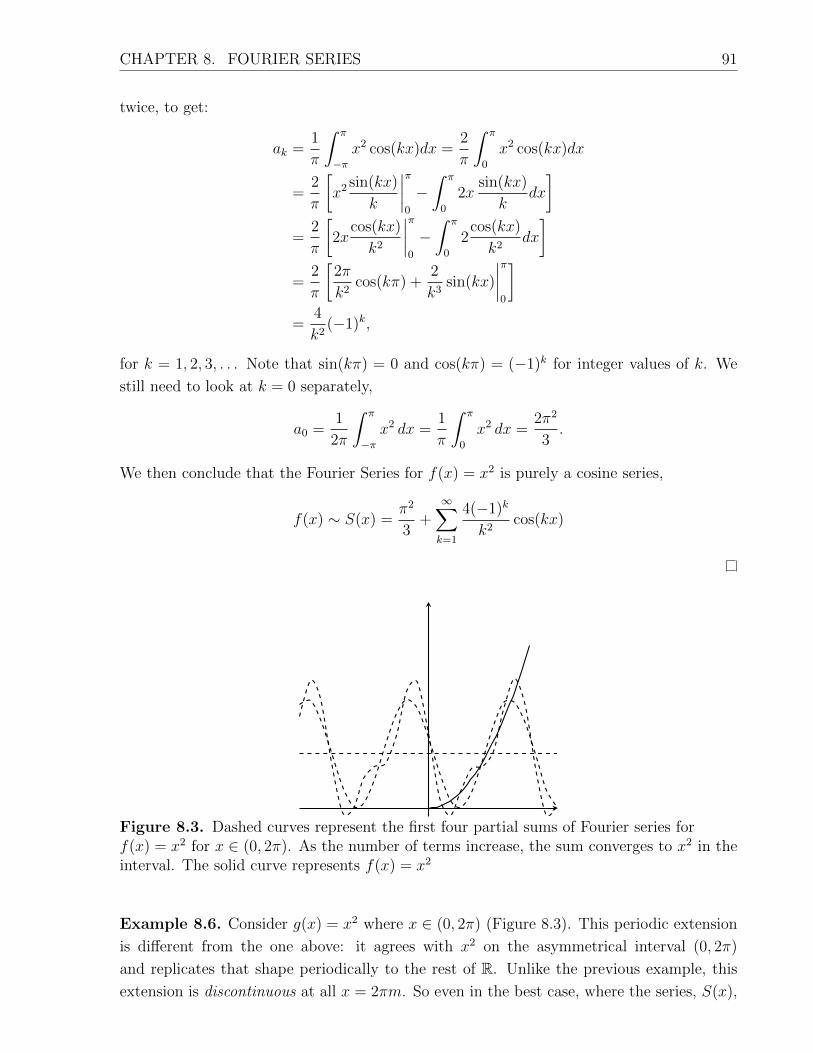
CHAPTER 8. FOURIER SERIES 91
twice, to get:
ak =1
π
∫ π
−πx2 cos(kx)dx =
2
π
∫ π
0
x2 cos(kx)dx
=2
π
[x2
sin(kx)
k
∣∣∣∣π0
−∫ π
0
2xsin(kx)
kdx
]=
2
π
[2x
cos(kx)
k2
∣∣∣∣π0
−∫ π
0
2cos(kx)
k2dx
]=
2
π
[2π
k2cos(kπ) +
2
k3sin(kx)
∣∣∣∣π0
]=
4
k2(−1)k,
for k = 1, 2, 3, . . . Note that sin(kπ) = 0 and cos(kπ) = (−1)k for integer values of k. We
still need to look at k = 0 separately,
a0 =1
2π
∫ π
−πx2 dx =
1
π
∫ π
0
x2 dx =2π2
3.
We then conclude that the Fourier Series for f(x) = x2 is purely a cosine series,
f(x) ∼ S(x) =π2
3+∞∑k=1
4(−1)k
k2cos(kx)
Figure 8.3. Dashed curves represent the first four partial sums of Fourier series forf(x) = x2 for x ∈ (0, 2π). As the number of terms increase, the sum converges to x2 in theinterval. The solid curve represents f(x) = x2
Example 8.6. Consider g(x) = x2 where x ∈ (0, 2π) (Figure 8.3). This periodic extension
is different from the one above: it agrees with x2 on the asymmetrical interval (0, 2π)
and replicates that shape periodically to the rest of R. Unlike the previous example, this
extension is discontinuous at all x = 2πm. So even in the best case, where the series, S(x),

CHAPTER 8. FOURIER SERIES 92
converges everywhere, it’s discontinuous function at x = 2πm, for all m ∈ Z. Still, does it
converge there, and if so, to which values?
We calculate the Fourier coefficients, but now over the non-symmetric interval (0, 2π).
Since the interval is not symmetric, we cannot assume either family of coefficients vanishes,
and indeed we have
a0 =1
2π
∫ 2π
0
x2dx = 8π2/3,
ak =1
π
∫ 2π
0
x2 cos(kx)dx = 4/k2,
bk =1
π
∫ 2π
0
x2 sin(kx)dx = −4π/k,
k = 1, 2, 3, . . . We don’t get the same Fourier Series, but then again this is not the same
function! The Fourier Series for x2 depends on the domain, since it only samples x2 over an
interval, and then replicates its values periodically to fill out all of x ∈ R.
Example 8.7. Consider f(x) = x where x ∈ (−π, π) and L = π (Figure 8.4). Then, we get
ak =1
π
∫ π
−πx cos(kx)dx = 0
bk =1
π
∫ π
−πx sin(kx)dx
=2
π
∫ π
0
x sin(kx)dx
=2
k(−1)k+1
So as f(x) = x on (−π, π) is odd, we have a sine series:
f(x) ∼ S(x) =∞∑k=1
2(−1)k+1
ksin(kx)
S(x) has discontinuities, f(−π) = −π 6= π = f(π). So what happens at the discontinu-
ities, x = (2m− 1)π?
S(nπ) =∞∑k=1
2(−1)k+1
ksin(knπ) =
∞∑k=1
0 = 0
It will be a general fact that at a jump discontinuity, the Fourier series, S(x), takes the
midpoint value. It does not choose the value of f(x) from either the right or the left at a
jump discontinuity.
8.4 Pointwise and Uniform Convergence
Let’s talk with convergence; not only is it interesting and important, but it goes to the heart
of what we get when we use Fourier Series to approximate a function. First, let’s review
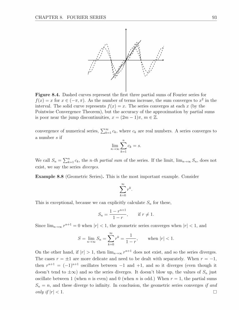
CHAPTER 8. FOURIER SERIES 93
Figure 8.4. Dashed curves represent the first three partial sums of Fourier series forf(x) = x for x ∈ (−π, π). As the number of terms increase, the sum converges to x2 in theinterval. The solid curve represents f(x) = x. The series converges at each x (by thePointwise Convergence Theorem), but the accuracy of the approximation by partial sumsis poor near the jump discontinuities, x = (2m− 1)π, m ∈ Z.
convergence of numerical series,∑∞
k=1 ck, where ck are real numbers. A series converges to
a number s if
limn→∞
n∑k=1
ck = s.
We call Sn =∑n
k=1 ck, the n-th partial sum of the series. If the limit, limn→∞ Sn, does not
exist, we say the series diverges.
Example 8.8 (Geometric Series). This is the most important example. Consider
∞∑k=0
rk.
This is exceptional, because we can explicitly calculate Sn for these,
Sn =1− rn+1
1− r , if r 6= 1.
Since limn→∞ rn+1 = 0 when |r| < 1, the geometric series converges when |r| < 1, and
S = limn→∞
Sn =∞∑k=0
rk =1
1− r , when |r| < 1.
On the other hand, if |r| > 1, then limn→∞ rn+1 does not exist, and so the series diverges.
The cases r = ±1 are more delicate and need to be dealt with separately. When r = −1,
then rn+1 = (−1)n+1 oscillates between −1 and +1, and so it diverges (even though it
doesn’t tend to ±∞) and so the series diverges. It doesn’t blow up, the values of Sn just
oscillate between 1 (when n is even) and 0 (when n is odd.) When r = 1, the partial sums
Sn = n, and these diverge to infinity. In conclusion, the geometric series converges if and
only if |r| < 1.

CHAPTER 8. FOURIER SERIES 94
Example 8.9 (p-series).∞∑k=1
1/kp converges iff p > 1.
This may be verified using the Integral Test (see Stewart!) Unlike the geometric series,
we don’t have a value to which the series converges– at least not yet! We will see that using
Fourier Series we may derive actual numerical values for some numerical series!
Using the comparison test, we can determine convergence and divergence of many series
using these examples.
Theorem 8.10 (Comparison Test). Assume that 0 ≤ ak ≤ bk for all k ∈ N.
• If∑∞
k=1 bk converges, then∑∞
k=1 ak also converges.
• If∑∞
k=1 ak diverges, then∑∞
k=1 bk also divverges.
Example 8.11. The series∑∞
k=11
2k2+k+1converges, since ak = 1
2k2+k+1≤ 1
2k2and
∑∞k=1
12k2
=12
∑∞k=1
1k2
converges (p-series with p = 2.)
The series∑∞
k=1k
2k2+k+1diverges, since k + 1 ≤ 2k2 for k ≥ 1, and so bk = k
2k2+k+1≥
k4k2
= 14k
and∑∞
k=114k
diverges (p-series with p = 1.)
While the Comparison Test and p-series concern series with positive terms, Fourier Series
contain sines and cosines, and so will have terms changing in sign. We distinguish two types
of convergence for series with sign-changing terms:
Definition 8.12 (Absolute and conditional convergence). A series∑∞
k=1 ck converges ab-
solutely if∑∞
k=1 |ck| converges. The series converges conditionally if∑∞
k=1 ck converges but∑∞k=1 |ck| diverges.
Basically, a conditionally convergent series depends on cancellation between positive and
negative terms to converge, while an absolutely convergent series is more robust: its terms
tend to zero rapidly enough to ensure convergence without having to count on cancellations.
Example 8.13 (Alternating series). The series
∞∑k=1
(−1)k1
kp(8.5)
alternates in sign, because of the (−1)k factor. If p > 1, then |ak| = 1/kp, and the p-series∑∞k=1 converges; thus for p > 1 this alternating series converges absolutely. On the other
hand, when 0 < p ≤ 1 the series of the absolute values is a divergent p-series, and so the
series (8.5) does not converge absolutely. However, any alternating series,
∞∑k=1
(−1)kbk, with limk→∞
bk = 0 and bk+1 ≤ bk for all k,
is convergent. (See Stewart.) Thus, the series (8.5) converges conditionally when 0 < p ≤ 1;
the terms tend to zero, but not rapidly enough for the series to converge without the help
of cancellation.

CHAPTER 8. FOURIER SERIES 95
For absolutely convergent series we can have a good estimate on the rate of convergence,
ie, how many terms we need to keep to have a good approximation of the limit by a partial
sum. On the other hand, conditional convergence is delicate and the series converges slowly.
Let’s apply these ideas to trigonometric Fourier series. For simplicity, we take L =
π, and consider 2π-periodic functions f(x) (which means extending functions on (−π, π)
periodically!), with the usual formula for the coefficients,
a0 =1
π
∫ π
−πf(x)dx
ak =1
π
∫ π
−πf(x) cos (kx) dx
bk =1
π
∫ π
−πf(x) sin (kx) dx,
(8.6)
k = 1, 2, 3, . . . The same facts will be true for 2L-periodic functions (with coefficients given
by (??)), but the messy formulas will obscure the ideas.
An important distinction is that Fourier series are series of functions, and not just
numbers:
S(x) =a02
+∞∑k=1
(ak cos(kx) + bk sin(kx)) =∞∑k=0
gk(x).
There are several different (and important) notions of convergence for series of functions.
The first is easy to grasp: For each fixed value of x,∑∞
k=1 gk(x) is a numerical series, which
converges or doesn’t. So we can ask for each individual x whether the series converges or
diverges.
Definition 8.14 (Pointwise convergence). We say that the series∑∞
k=1 gk(x) converges
pointwise on a set A ∈ R if the series converges for every individual x ∈ A.
The notion of poinwise convergence is simple and easy to verify, but it has some draw-
backs. In particular, series of continuous functions might converge pointwise to a discontin-
uous limit function. Also, differentiating or integrating a pointwise convergent series might
lead to incorrect answers.
Example 8.15. Consider∞∑k=1
(1− x)xk, x ∈ [0, 1].
Then, we get the following partial sums:
Sn =n∑k=1
(1− x)xk = (1− x)n∑k=1
xk.
If x ∈ [0, 1), the series converges:
limn→∞
Sn(x) = (1− x) limn→∞
n∑k=1
xk︸ ︷︷ ︸1/(1−x)
= 1

CHAPTER 8. FOURIER SERIES 96
However, when x = 1, we have Sn(1) = 0. So at x = 1, the series converges to 0, i.e.
∞∑k=1
(1− x)xk =
{1 if x ∈ [0, 1)
0 if x = 1
Therefore, the series converges pointwise on the set A = [0, 1]. Notice that, although each
partial sum Sn(x) is a continuous function on A, the series converges to a discontinuous
limit function!
A series of continuous functions can converge pointwise to a discontinuous function, and
there are examples for which the series of the integrals is not equal to the integral of the
series, ∫ b
a
(∞∑k=1
gn(x)
)dx 6=
∞∑k=1
∫ b
a
gn(x)dx.
(Notice that when we calculated the Fourier coefficients in (8.4) we were implicitly assuming
these would be equal!) So we need to be very careful about doing calculus with a series
which is only pointwise convergent.
Fortunately, there is a nice theorem about pointwise convergence of trigonometric Fourier
series, which is easy to apply. (However, it is fairly tricky to prove!)
Definition 8.16. We say that f(x) is piecewise C1, or piecewise smooth, on [a, b] if (i) f
is differentiable and f ′(x) is continuous except maybe at finitely many points; (ii) At each
exceptional point, f(x) and f ′(x) have jump discontinuities.
At a jump discontinuity x, we denote the left- and right-hand limits by:
f(x+)
= limt→x+
f(t),
f(x−)
= limt→x−
f(t).
Recall that f is continuous at x if and only if f (x+) = f(x) = f (x−) .
We need to be careful with this definition when dealing with Fourier Series, because even
if f is C1([−π, π]), when we construct a Fourier series we get the 2π-periodic extension of
f to R, which might create discontinuities. We saw this happen in Examples 8.6 and 8.7.
Theorem 8.17 (Pointwise Convergence Theorem for Trigonometric Fourier Series). Assume
f is a piecewise C1, (2π)-periodic function. Then, its trigonometric Fourier Series,
S(x) =a02
+∞∑k=1
[ak cos(kx) + bk sin(kx)] ,
(with coefficients given by (8.6)) converges pointwise at every x ∈ R to
S(x) =1
2
(f(x+)
+ f(x−)).
CHAPTER 8. FOURIER SERIES 97
In other words, if f is continuous, S(x) = f(x). If f(x) jumps, S(x) averages the jump
values.
Remark. It is not sufficient to assume f is continuous to conclude that
limn→∞
Sn(x) = f(x),
some additional information is needed. There are examples of functions which are continuous
(but not piecwise C1) for which the Fourier Series diverges at some values of x.
Example 8.18. Consider f(x) = x, x ∈ (−π, π). Then,
S(x) =∞∑k=1
2(−1)k+1
ksin(kx)
= x,
if x ∈ (−π, π), and S(kπ) = 0 for each k ∈ Z, which averages the value across the jump
discontinuities in the 2π-periodic extension of f .
Example 8.19. Consider f(x) = x for x ∈ (−π, π), which is extended 2π-periodically. We
already calculated its Fourier Series,
S(x) =∞∑k=1
2(−1)k+1
ksin(kx).
Then, f(x) is piecewise C1, but it is discontinuous on R, since it must jump at odd multiples
of π in order to be periodic. So by the Pointwise Convergence Theorem, it converges at all
values x ∈ R, and agrees with the periodic extension for x 6= (2m− 1)π, m ∈ Z. At the odd
multiples of π, the Fourier Series takes the midpoint value at the discontinuity,
S ((2m− 1)π) =∞∑k=1
2(−1)k+1
ksin(0) =
∞∑k=1
0 = 0.
Observe that bk is an alternating sequence, and
|bk| =∣∣∣∣2(−1)k+1
k
∣∣∣∣ =2
k.
Since∑∞
k=1 2/k diverges, the series converges conditionally. We can see how slowly it
converges by looking at graphs of Sn, for large n.
Example 8.20. Consider f(x) = x2 with x ∈ (−π, π) extended 2π-periodically. In this
case, the extension is piecewise C1 and also continuous, so the Fourier Series converges to
the periodic extension at all values of x, S(x) = f(x)∀x ∈ R. Further, we find that
S(x) =π2
3+∞∑k=1
4(−1)k
k2cos(kx).

CHAPTER 8. FOURIER SERIES 98
Then, by looking at the individual terms,
|ak cos(kx)| =∣∣∣∣4(−1)k
k2cos(kx)
∣∣∣∣ ≤ 4
k2,
we find that S(x) converges absolutely for all x ∈ R by the Comparison Test.
Since it converges for all x ∈ R, let’s try some values. First, when x = 0, we get
π2
3+∞∑k=1
4(−1)k
k2= 0
So we find that∞∑k=1
(−1)k
k2= −π
2
12
Likewise, when x = π, we find that
∞∑k=1
1
k2=π2
6
In this way Fourier Series provides us with some exact numerical values for some common
series.
This example illustrates a second notion of convergence, uniform convergence. A uni-
formly convergent series is one for which the partial sums Sn(x) approximate the limiting
function S(x) to within the same error at all points x. If you were to draw a thin strip of
uniform width around the graph y = S(x), the graphs y = Sn(x) would all fit completely in-
side the strip for n large. Figure 8.5 shows how closely the Fourier partial sums approximate
x2 on [−π, π].
-4 -3.2 -2.4 -1.6 -0.8 0 0.8 1.6 2.4 3.2 4
2.5
5
7.5
10
Figure 8.5. Partial sums Sn for n = 3, 5, 15, 50 for f(x) = x2 on (−π, π). Theconvergence is uniform.
Theorem 8.21 (Uniform Convergence). Consider S(x) =∑∞
k=1 gk(x) with x ∈ [a, b]. We
say that the series converges uniformly to S(x) if
limn→∞
(maxx∈[a,b]
∣∣∣∣∣S(x)−n∑k=1
gk(x)
∣∣∣∣∣)
= 0.

CHAPTER 8. FOURIER SERIES 99
In other words, for any ε > 0, there is an N for which∣∣∣∣∣S(x)−n∑k=1
gk(x)
∣∣∣∣∣ < ε for all x ∈ [a, b],
whenever n ≥ N .
This looks a bit complicated, but fortunately there is a test for uniform convergence
which is easy to apply; it strongly resembles the Comparison Test for numerical series!
Theorem 8.22 (Weierstress). Assume gk(x) are continuous on [a, b], where k = 1, 2, 3, . . . .
• M-Test. If |gk(x)| < Mk, for all x ∈ [a, b], and∑
kMk converges, then∑
k gk(x)
converges uniformly on [a, b].
• If S(x) =∑
k=1 gk(x) converges uniformly on [a, b], then S(x) is continuous, and∫ b
a
S(x)dx =∞∑k=1
∫ b
a
gk(x)dx
When you study Real Analysis you will prove this theorem (which actually is not very
difficult!)
Going back to our favorite examples, the series for f(x) = x can not converge uniformly,
because f(x) = x extended 2π-periodically is discontinuous, contrary to the Weierstrass
theorem. On the other hand, the series for f(x) = x2 extended 2π-periodically does converge
uniformly, because
|gk(x)| =∣∣∣∣4(−1)k
k2cos(kx)
∣∣∣∣ ≤ 4
k2∀x ∈ R,
and the numerical series∑∞
k=14k2
converges (it’s the p-series with p = 2.) So we can apply
Weierstrass’ M-Test with Mk = 4k2
and conclude that the Fourier Series converges uniformly.
For Fourier Series applying Weierstrass’ M-Test for uniform convergence is particularly
easy, since the variable part of the terms in the series are always sin(kx) or cos(kx), and
these are easily bounded,
| sin(kx)| ≤ 1, | cos(kx)| ≤ 1 for all x ∈ R.
Thus, we may always compare the terms of a trigonometric Fourier Series with the numerical
series defined by the abolute value of the coefficients,
|gk(x)| = |ak cos(kx) + bk sin(kx)| ≤ |ak| | cos(kx)|+ |bk| | sin(kx)| ≤ |ak|+ |bk|,
for all x ∈ R. Therefore, the Weierstrass M -Test reduces to the absolute convergence of the
series of the coefficients, ak, bk:

CHAPTER 8. FOURIER SERIES 100
Corollary 8.23. Suppose the absolute values of the Fourier coefficients ak, bk are summable,
that is∞∑k=1
(|ak|+ |bk|) converges.
Then the Fourier Series S(x) = a02
+∑∞
k=1 ak cos(kx) + bk sin(kx) converges uniformly on
R.
From the second part of Theorem 8.22 this can only happen when the 2π-periodic ex-
tension of f is continuous.
Example 8.24. Consider f(x) = | sinx| with x ∈ (−π, π). The 2π-periodic extension is
even, piecewise C1, and continuous (graph it, either by hand or using the computer!) Then,
because f is even, we must have the sine coefficients vanish, bk = 0 for all k ∈ N. For the
cosine coefficients we use the evenness of f to eliminate the absolute value,
ak =1
π
∫ π
−π| sinx| cos(kx) dx
=2
π
∫ π
0
| sinx| cos(kx) dx (f is even)
=2
π
∫ π
0
sinx cos(kx) dx (sinx ≥ 0 when 0 ≤ x ≤ π)
=1
π
∫ π
0
[sin(1 + k)x+ sin(1− k)x] dx
=1
π
[cos(1 + k)x
(1 + k)+
cos(1− k)x
(1− k)
]π0
(if k 6= 1!)
=1
π
[cos(1 + k)π − 1
(1 + k)+
cos(1− k)π − 1
(1− k)
]=
(−1)k+1 − 1
π
[1
k + 1− 1
k − 1
]=
2
π
((−1)k+1 − 1
) 1
k2 − 1
=
{− 4π
14j2−1 , if k = 2j is even;
0, if k is odd.
When k = 1, we notice that the second term in the integral in the 4th line is zero, and the
first term integrates to zero as well, so a1 = 0. When k = 1 there is no division by zero, and
so the a0 term has already been calculated with the other ak, a0 = 4/π. The only surviving
terms in the series are ak with k = 2j an even counting number. Therefore, we re-index the
series, counting only the even terms, a2j, j ∈ N,
S(x) =2
π− 4
π
∞∑j=1
1
4j2 − 1cos(2jx),
which converges for each individual x to f(x) by the Pointwise Convergence Theorem.

CHAPTER 8. FOURIER SERIES 101
Since
|a2j| =∣∣∣∣− 4
π
1
4j2 − 1
∣∣∣∣=
4
π(4j2 − 1)
≤ 4
π
1
4j2 − j2 =4
3π
1
j2,
and∑
1/j2 converges, the series converges uniformly according to Weierstrass’ M-Test. (See
figure 8.6.)
We can now use it to calculate some numerical series. When x = 0, by the pointwise
convergence theorem,
0 = f(0) =2
π− 4
π
∞∑j=1
1
4j2 − 1,
and so we find the value of another numerical series,
∞∑j=1
1
4j2 − 1=
1
2
When x = π2, since cos(2jx) = cos(πx) = (−1)j, we obtain an alternating numerical
series thanks to the pointwise convergence theorem,
1 = | sin(π
2)| = f
(π2
)=
2
π− 4
π
∞∑j=1
(−1)j
4j2 − 1.
Rearranging terms,∞∑j=1
(−1)j
4j2 − 1=π
4
[2
π− 1
]=
1
2− π
4.
-4 -3.2 -2.4 -1.6 -0.8 0 0.8 1.6 2.4 3.2 4
0.5
1
Figure 8.6. Partial sums Sn for n = 3, 5, 15, 50 for f(x) = | sinx| on (−π, π). Theconvergence is uniform.

CHAPTER 8. FOURIER SERIES 102
8.5 Orthogonal families
Fourier Series is fundamentally about orthogonality, representing functions in an orthogonal
basis. Cosines and sines give only one example of orthogonal families of functions. So where
else do orthogonal functions come from? Here are two mechanisms which produce orthogonal
families of functions, which are useful and natural in various contexts.
8.5.1 The Gram-Schmidt process
Take a linearly independent collection {v1, v2, v3, . . . } in any vector space. The Gram-
Scmidt process gives an iterative procedure to create an orthogonal set {u1, u2, u3 . . . } by
orthogonal projection, which spans the same space as the original collection. (See section
6.3 in Anton & Rorres [AR] to review this concept.)
Take u1 = v1. Then,
u2 = v2 −〈v2, u1〉‖u1‖2
u1
is orthogonal to u1. To see this, just take the inner product:
〈u1, u2〉 = 〈u1, v2〉 −⟨u1〈v2, u1〉‖u1‖2
u1
⟩= 〈u1, v2〉 −
〈v2, u1〉‖u1‖2
〈u1, u1〉︸ ︷︷ ︸‖u1‖2
= 0.
We then iterate the preceeding step, and create the orthogonal family by induction.
Assume we already have an orthogonal family with k elements,
{u1, u2, . . . , uk}.
Then, the vector obtained by subtracting off the projections onto the previous orthogonal
elements,
uk+1 = vk+1 −k∑j=1
〈vj+1, uj〉‖uj‖2
uj
is orthogonal to {u1, u2, . . . , uk}, and will have the same span as {v1, v2, . . . , vk+1}.A common application is to polynomials, P (x) = a0 + a1x + · · · + anx
n. A basis of
polynomials is {1, x, x2, . . . }. For any choice of inner product, we get different orthogonal
families of polynomials (named after Legendre, Chebyshev, Bernstein . . . ,) and useful in
approximation theory and numerical analysis.
Example 8.25. Take the vector subspace of polynomials, that is the linearly independent
set
{1, x, x2, , . . . , xk, . . . },

CHAPTER 8. FOURIER SERIES 103
on the interval x ∈ [−1, 1]. We choose the familiar L2 inner product,
〈f, g〉 =
∫ 1
−1f(x)g(x)dx.
Start with P0(x) = 1, the constant function. In Problem #12 below, you’ll verify that
P1(x) = x and P1(x) ⊥ P0(x). Continuing with Gram-Schmidt, we get the next orthogonal
element,
P2(x) = x2 − 〈x2, P0〉‖P0‖2
P0 −−〈x2, P1〉‖P1‖2
P1
= x2 −∫ 1
−1 x2 · 1dx∫ 1
−1 12dx−∫ 1
−1 x3 · 1dx∫ 1
−1 x2dx︸ ︷︷ ︸
=0
= x2 − 1
3.
This procedure generates the Chebyshev polynomials on [−1, 1], which are very often used
in numerical analysis.
To get other families, we can substitute a different inner product. A common choice is
a “weighted” inner product,
〈f, g〉 =
∫ 1
−1f(x)g(x)w(x)dx,
where w(x) is a given continuous function. The principle is the same as for the Chebyshev
polynomials, but changing the inner product will change the actual polynomials obtained
as an orthogonal family.
8.5.2 Eigenvalue problems
This mechanism for generating orthogonal families comes from the basic linear algebra
theorems about eigenvalues and eigenvectors of symmetric matrices. Recall that a matrix
is symmetric if its transpose M t = M . This is equivalent to symmetry with respect to the
inner (dot) product, (M~u) ·~v = ~u ·(M~v), for all vectors ~u,~v ∈ Rn. In a general inner product
space V this is the appropriate way to talk about symmetry:
Definition 8.26. Let M be a linear transformation on an inner product space V. We say
M is symmetric if
〈Mu, v〉 = 〈u,Mv〉, for all u, v ∈ V .Theorem 8.27. Let M be a symmetric linear transformation on an inner product space V.
If Mu = λu and Mv = µv with distinct eigenvalues λ 6= µ, then 〈u, v〉 = 0.
Proof. Notice that due to symmetry, we get
〈λu, v〉 = 〈Mu, v〉 = 〈u,Mv〉 = 〈u, µv〉
So we get λ〈u, v〉 = µ〈u, v〉. So since λ 6= µ, we conclude that 〈u, v〉 = 0.

CHAPTER 8. FOURIER SERIES 104
In Rn, any symmetric linear transformation (i.e. matrix) provides an orthogonal basis
of eigenvectors of M for Rn. Even though V is infinite dimensional, it turns out that this is
still true in the sense of Fourier series.
Now, consider a vector space V of all C2 functions,
u : [0, L]→ R,
satisfying a boundary condition,
u(0) = 0 and u(L) = 0.
(Note the similarity to the class of admissible variations, A0 from the last chapter!) On the
vector space V we use the familiar inner product 〈u, v〉 =∫ L0u(x)v(x)dx.
Now consider the transformation Mu = u′′(x), which takes u ∈ V and gives back its
the second derivative. By the usual properties of the derivative, if u1, u2 ∈ V and c1, c2 are
constants, then
M(c1u1 + c2u2) =d2
dx2(c1u1 + c2u2) = c1u
′′1(x) + c2u
′′2(x) = c1Mu1 + c2Mu2,
and so indeed M is a linear transformation on this vector space V .
Lemma 8.28. M is symmetric with respect to the inner product on V.
Proof. We integrate by parts, twice:
〈Mu, v〉 =
∫ L
0
u′′(x)v(x)dx
= u′(x)v(x)|L0 −∫ L
0
u′(x)v′(x)dx
= −v′(x)u(x)|L0 +
∫ L
0
u(x)v′′(x)dx
= 〈u,Mv〉
As in the Calculus of Variations, the endpoint terms all vanish because u, v vanish at
x = 0, L.
In particular, by Lemma 8.27 eigenvectors of the transformation M must be orthogonal
if their eigenvalues are distinct. But what are the eigenvectors of a linear transformation
like M? Just as for matrices, λ ∈ R is an eigenvalue of M if there exists a nonzero element
u ∈ V , u 6= 0 such that Mu = λu. In this context, finding eigenvalues involves solving
an ordinary differential equation (ODE) with boundary conditions which define the vector
space V , u(0) = 0 = u(L). In this case, we refer to u(x) as an eigenfunction of M . One way
to do this is to find all solutions of the ODE with the left-hand boundary value u(0) = 0
as an initial condition, and check to see if they also solve the right-hand boundary value

CHAPTER 8. FOURIER SERIES 105
u(L) = 0. When finding the general solution to the ODE we have 3 cases to consider,
λ > 0, λ = 0, λ < 0, since the form of the general solution to the ODE is different in each
case.
When λ > 0, the general solution to the ODE is
u(x) = A cosh√λx+B sinh
√λx.
Since we need u(0) = 0, we must have A = 0. To satisfy the other boundary condition,
0 = u(L) = sinh√λL, but sinhx > 0 whenever x > 0 so this can never be satisfied except
when B = 0 also. So we only get the trivial solution u(x) ≡ 0, and so there is no eigenvalue
with λ > 0.
Similarly, when λ = 0 the general solution to the ODE, Mu = u′′(x) = 0 is u(x) =
A + Bx, and the only straight line with u(0) = 0 = u(L) is the trivial one u(x) ≡ 0. So
λ = 0 is not an eigenvalue either.
We conclude that for all eigenvalues λ < 0. For convenience, call λ = −µ2 with µ > 0.
Then u′′ + µ2u = 0 with general solution
u(x) = A cosµx+B sinµx.
Applying the condition u(0) = 0, we have A = 0 as before. But at the other endpoint we
have nontrivial solutions:
0 = u(L) = B sinµL
is solved when µL = kπ, k ∈ N, that is µ = µk = kπL
. So we get a sequence of eigenvalues
and associated eigenfunctions,
λk = −µ2k =
k2π2
L2, uk(x) = sin
(kπx
L
).
By Lemma 8.28 these form an orthogonal family of functions on [0, L]. And given f :
[0, L]→ R we can make a Fourier expansion in this family,
f(x) ∼ S(x) =∞∑k=1
ckφk(x),
where
ck =〈f, φk〉‖φk‖2
,
and the norm is defined via the inner product as usual, ‖f‖ =√〈f, f〉. As for the full
trigonometric Fourier Series (sines and cosines), in what sense are f(x) and S(x) equal, and
does the series converge?

CHAPTER 8. FOURIER SERIES 106
8.6 Convergence in Norm
We return to questions of convergence of Fourier Series, this time including all orthogo-
nal expansions and not just the classical trigonometric series. The most natural kind of
convergence involves the norm ‖v‖ on the vector space of functions v ∈ V .
As always, we define the partial sums,
Sn(x) =n∑k=1
ckφk(x). (8.7)
Definition 8.29. We say the series (8.7) converges in norm if
limn→∞
‖Sn − f‖ = 0.
In many cases, the scalar product and norm are defined by definite integrals,
〈f, g〉 =
∫ b
a
f(x) g(x), dx, ‖f‖ =√〈f, f〉 =
√∫ b
a
[f(x)]2 dx.
These quantities are well-defined for continuous f , but as we’ve seen, we are often interested
in discontinuous functions as well. So it is natural to open up the possibilty of discontinuous
f , as long as the integral defining the norm makes sense (and is finite.) We say a function is
square integrable if ‖f‖ <∞. (A historically important question in analysis was to identify
the proper condition for square integrability, solved by Lebesgue in his theory of integration
in 1904!)
Definition 8.30. We call the family {φk(x)} complete if for all square integrable functions
f , the series (8.7) converges to f in norm, that is, limn→∞
‖Sn − f‖ = 0.
Thus, to say the orthogonal family {φk(x)} is complete essentially means that it forms
an orthogonal basis for all square integrable f(x) on [a, b]. This definition just gives a
name to a desirable property of orthogonal families. Given a family of orthogonal functions
{φk}, one must show that it is (or isn’t) complete, using properties of those functions. It
turns out that the two types of examples discussed in the previous section, the Legendre
polynomials on [−1, 1] from Section 8.5.1 and eigenfunctions of symmetric boundary-value
problems from Section 8.5.2, both yield complete sets of orthogonal functions. Proving this
is a difficult question in analysis, and we won’t address it here.
Nevertheless, let’s look at some simple consequences of measuring convergence via the
norm. First, let’s use orthogonality to actually calculate the square of the error made in

CHAPTER 8. FOURIER SERIES 107
approximating f by Sn in the norm. (We have to be careful about indices!)
‖Sn − f‖2 = 〈Sn − f , Sn − f〉 =
⟨[n∑k=1
ckφk − f],
[n∑j=1
cjφj − f]⟩
=
⟨n∑k=1
ckφk ,
n∑j=1
cjφj
⟩− 2
⟨n∑k=1
ckφk , f
⟩+ ‖f‖2
=n∑k=1
n∑j=1
ckcj〈φk, φj〉+ 2n∑k=1
ck〈φk, f〉+ ‖f‖2
=n∑k=1
c2k‖φk‖2 − 2n∑k=1
c2k‖φk‖2 + ‖f‖2
= ‖f‖2 −n∑k=1
c2k‖φk‖2.
We draw two conclusions from this computation. The first comes from the observation that
the norm ‖Sn − f‖2 ≥ 0, and so the infinite series
∞∑k=1
c2k‖φk‖2 = limn→∞
n∑k=1
c2k‖φk‖2 ≤ ‖f‖2 <∞,
so that numerical series∑n
k=1 c2k‖φk‖2 converges, to something at most ‖f‖2. This fact is
called Bessel’s inequality. The second conclusion is that the Fourier Series converges in
norm if and only if
0 = limn→∞
‖f − Sn‖2 = limn→∞
[‖f‖2 −
n∑k=1
c2k‖φk‖2]
= ‖f‖2 −∞∑k=1
c2k ‖φk‖2 ,
that is, if equality holds in Bessel’s inequality. So, provided the family {φk} is complete,
there is a relationship between the norm of the function f and its Fourier coefficients with
respect to {φk}, called Parseval’s identity,
‖f‖2 =∞∑k=1
c2k ‖φk‖2 .
Classical Fourier Series, based on the orthogonal family of trigonometric functions,
{1, cos(kx), sin(kx) | k = 1, 2, 3, . . . },
is known to be complete, and so any square-integrable function f on [−π, π] may be ex-
panded in a Fourier Series which converges in norm:
Theorem 8.31 (Parseval’s Theorem). Suppose f(x) is defined on [−π, π] and∫ π
−π(f(x))2 dx <∞.

CHAPTER 8. FOURIER SERIES 108
Then, the trigonometric Fourier Series of f(x),
S(x) =a02
+∞∑k=1
(ak cos(kx) + bk sin(kx))
converges to f(x) in norm on [−π, π]. In addition,
∫ π
−π(f(x))2 dx = π
[a202
+∞∑k=1
(a2k + b2k
)](8.8)
The formula (8.8) is known as Parseval’s Identity. The proof of Parseval’s Theorem is
quite intricate, and not appropriate for a course of this level. However, we may appreciate
what it says about convergence of Fourier Series, and use it calculate exact values for some
more numerical series.
Example 8.32. Consider f(x) = x with x ∈ [−π, π]. We calculated the coefficients in
Example 8.7, and discussed its convergence in Example 8.19. In particular, we noted that
it converges pointwise at every x ∈ R, although it converges to the midpoint of the jump
discontinuities at odd multiples of π, and since it is discontinuous as a 2π-periodic function
on R, it cannot converge uniformly. On the other hand, f(x) = x is square integrable on
[−π, π], and so its trigonometric Fourier Series does converge in norm. In particular, this
shows that convergence in norm is weaker than uniform convergence: a series may converge
in norm without converging uniformly. Also, convergence in norm permits the series to differ
from f(x) at points of discontinuity. From the calculated values of the Fourier coefficients,
ak = 0, bk =2
k(−1)k+1,
and Parseval’s identity we then obtain an explicit value for a numerical series:
π∞∑k=1
4
k2=
∫ π
−πx2dx =
2
3π3
∞∑k=1
1
k2=π2
6.
Returning to Example 8.24, f(x) = | sinx| for x ∈ (−π, π), and extended as a 2π-periodic
function, we had (by evenness) bk=0 for all k, and
ak =
{− 4π
14j2−1 , if k = 2j is even;
0, if k is odd.

CHAPTER 8. FOURIER SERIES 109
Applying Parseval’s theorem, we then get the identity,
1
2a20 +
∞∑j=1
a22j =1
2
(2
π
)2
+
(4
π
)2 ∞∑j=1
1
(4j2 − 1)2
=1
π
∫ π
−π| sinx|2 dx
=1
π
∫ π
−π
1
2[1− cos(2x)] dx
= 1.
And so we can evaluate the infinite series,
∞∑j=1
1
(4j2 − 1)2=π2
16− 1
8.
You can go back to each of the examples we’ve calculated in class or in the practice problems
and apply Parseval’s identity to the coefficients to obtain some new identites which give
explicit values to various series.
8.7 Application: The vibrating string
To conclude, we look at a problem which is very similar to Fourier’s original motivation,
the solution of partial differential equations arising in science. Instead of the heat equation,
let’s look instead at the wave equation, which describes a vibrating string.
Consider a string in a violin, guitar, piano, etc. with length L. Suppose that the string
is attached at its endpoints, x = 0, L, but is free to vibrate up and down in a vertical plane
in between. We call u(x, t) the shape of the string at the point x and time t, so we imagine
a snapshot of the string at time t giving us a graph y = u(x, t). The fact that the string is
attached at the endpoints means that we are imposing boundary conditions,
u(0, t) = 0, u(L, t) = 0, for all time t ∈ R. (8.9)
The equation of motion for the string is the wave equation,
∂2u
∂t2= c2
∂2u
∂x2,
where c is a constant which depends on the density and tension of the string.
We can solve this using Fourier Series! Recall from section 8.5.2 that we obtain an
orthogonal family of eigenfunctions by solving a boundary-value problem. For the choice
(8.9), these are:
vk(x) = sin
(kπ
Lx
).

CHAPTER 8. FOURIER SERIES 110
So we seek a solution in the form of a Fourier Series with time-dependent coefficients,
u(x, t) =∞∑k=1
ak(t) vk(x).
This is already chosen to satisfy the boundary conditions, so we plug into the wave equation
to determine the equation satisfied by the coefficients ak(t) and get:
a′′k(t) = −(kπc
L
)2
ak(t),
which has as a general solution
ak(t) = Ak cos
(kπc
Lt+ φk
),
where φk is a phase factor.1
To understand what is going on, look at each individual term in the series,
ak(t) vk(x) = Ak cos
(kπc
Lt+ φk
)sin
(kπ
Lx
).
Each of these terms is a simple standing wave, associated to φk, a fixed wave form in x
multiplied by an oscillatory term in t which makes the wave move up and down but with a
fixed profile. The profile comes from vk(x), which has (k−1) nodes (zeros) inside the string
x ∈ (0, L); see figure 8.7. The time dependence determines the sound produced, which is a
single pure frequency:
ωk =kc
2L, k = 1, 2, 3, . . .
So each term k = 1, 2, 3, . . . produces a different musical note, and the entire wave makes a
sound which is a superposition of these different notes!
The k = 1 term gives the fundamental tone, ω1 = c/2L, the lowest note produced by
the string. For k = 2, 3, 4, . . . , we get ωk = kω1, the overtones.
Suppose the length, density, and tension in the string are chosen so that the fundamental
frequency ω1 = 440 Hz, which is A4, the A just above middle-C on a piano. Then, the first
overtone ω2 = 880 Hz gives A5, which is exactly one octave higher. The next overtone
ω3 = 1320 Hz is E6, which is a perfect fifth above A5. Continuing, ω4 is A6 (two octaves
above the fundamental tone ω1) and w5 is C#7 . When you play A4 on a stringed instrument
you are actually hearing a combination of the intended note with a bit of each overtone.
The same principle applies to woodwind instruments. The vibrating string becomes a
vibrating column of air, and u(x, t) is the fluctuation of air pressure away from atmospheric
pressure in the room. A flute is an air column which is open to the atmosphere on both
ends, and so it gives the same boundary condition (8.9) as for a stringed instrument, and
1You could write it as ak(t) = αk coskπcL t + βk sin
kπcL t, but by a trig identity the two expressions are
the same.

CHAPTER 8. FOURIER SERIES 111
k=1k=2
k=3k=4
k=5
Figure 8.7. The standing wave profiles vk for the first five harmonics of the vibratingstring. Higher frequencies mean more nodes (zeros) in the waveform.
therefore the same harmonic sequence of frequencies. However, clarinets are different: they
have an end with a mothpiece and a reed, which are not open to the atmosphere, where the
pressure is maximal. This changes the boundary condition at the end x = 0 to ux(0, t) = 0.
This eigenvalue problem is the subject of Problem 8, below! The consequence is that the
orthogonal basis is different, with different eigenvalues, and a completely different harmonic
sequence of overtones!
8.8 Practice problems
1. Find the Fourier Series on [−π, π] of the following functions: sin2 x, sinx cosx, sin3 x,
and sin4 x.
[Hint: you don’t need to calculate any integrals!]
2. Calculate the Fourier Series S(x) of f(x) = sin(x/2), −π < x < π. What is S(π) =?
3. Find the Fourier Series of f(x) = coshx and g(x) = sinhx, −1 < x < 1. What are the
values of the Fourier Series at x = −1?
4. Find the Fourier Series on (−π, π) of
f(x) =
{− cosx, if −π < x < 0,
cosx, if 0 < x < π.
At what points in R is the Fourier Series discontinuous?
5. (a) Show that {1, cos(kx) | k ∈ N} is an orthogonal family on [0, π] with inner product
〈f, g〉 =
∫ π
0
f(x) g(x) dx.
CHAPTER 8. FOURIER SERIES 112
(b) Find the formulas for the coefficients in a Fourier Series in these functions, f(x) ∼S(x) = a0
2+∑
k=1 ak cos(kx).
(c) Show that S(x) represents the even, 2π-periodic extension of f(x) from 0 < x < π
to the real line. Draw the graph of S(x) on −3π < x < 3π when f(x) = x.
6. (a) Calculate the Fourier Series of f(x) = |x|, −π < x < π.
(b) Draw the 2π-periodic function which the series converges to, over the interval
−3π < x < 3π.
(c) Does the series converge absolutely or conditionally? Does it converge uniformly?
Why or why not?
(d) Use your result to calculate∞∑k=1
1
(2k − 1)2and
∞∑k=1
1
(2k − 1)4.
7. Answer (a)–(c) for f(x) = cos(x/4), −π < x < π. Use the Fourier coefficients to obtain
explicit values for the series∞∑k=1
1
16k2 − 1,∞∑k=1
(−1)k
16k2 − 1, and
∞∑k=1
1
(16k2 − 1)2.
8. Answer (a)–(c) for f(x) = sin(x/4), −π < x < π. Use the Fourier coefficients to obtain
an explicit value for the series∞∑k=1
k2
(16k2 − 1)2.
9. Consider the vector space V of all C2 functions u : [0, L]→ R satisfying the boundary
conditions u′(0) = 0 and u(L) = 0, and the linear transformation Mu = u′′(x).
(a) Show that for any u, v ∈ V , 〈Mu, v〉 = 〈u,Mv〉.[Hint: integrate by parts twice, and use the boundary conditions.]
(b) Suppose λ, µ are eigenvalues of M , so there exist nontrivial functions u, v ∈ V , with
Mu = u′′(x) = λu(x) and Mv = v′′(x) = µv. Show that if λ 6= µ, then 〈u, v〉 = 0.
(c) Show that
{cos
((2k − 1)πx
2L
): k = 1, 2, 3, . . .
}are eigenfunctions of M with
distinct eigenvalues λk = −( (2k−1)π2L
)2, and conclude that they form an orthogonal family in
V .
10. (a) Find the Fourier Series S(x) of f(x) = cos(x/2), −π < x < π.
(b) Graph S(x) for −3π < x < 3π. Does S(x) represent a continuous function on R?
(c) Use (a) to evaluate∞∑n=1
1
4n2 − 1and
∞∑n=1
(−1)k
4n2 − 1.
11. Consider the family of functions
{φk(x) = sin
[(k +
1
2)x
], k = 0, 1, 2, 3, . . .
}on
x ∈ [−π, π].

CHAPTER 8. FOURIER SERIES 113
(a) Show that this family is orthogonal with respect to the inner product
〈f, g〉 =
∫ π
0
f(x)g(x) dx.
(b) Give the formula for Fourier coefficients for a function f(x) with respect to this
family,
f(x) ∼ S(x) =∞∑k=0
ckφk(x).
12. For x ∈ [−1, 1], define the polynomials,
P0(x) = 1, P1(x) = x, P2(x) = 3x2 − 1, P3(x) = 5x3 − 3x.
(a) Show that these four functions are orthogonal with respect to the inner product
〈f, g〉 =
∫ 1
−1f(x)g(x) dx.
(b) If f(x) = a0 + a1x + a2x2 + a3x
3 + · · · + anxn is a nontrivial polynomial of degree
n, and f is orthogonal to each of P0, P1, P2, P3, show that the degree n ≥ 4.
[Hints: Assume for a contradiction that n ≤ 3, so f(x) = a0 + a1x + a2x2 + a3x
3, and
show a0 = 0 = a1 = a2 = a3 (and so f(x) is the zero polynomial).]
(c) Find a polynomial P4(x) which is of order 4 and which is orthogonal to each of
P0, P1, P2, P3.